A machine-learning approach to synthesize virtual sensors for parameter-varying systems

Abstract

This paper introduces a novel model-free approach to synthesize virtual sensors for the estimation of dynamical quantities that are unmeasurable at runtime but are available for design purposes on test benches. After collecting a dataset of measurements of such quantities, together with other variables that are also available during on-line operations, the virtual sensor is obtained using machine learning techniques by training a predictor whose inputs are the measured variables and the features extracted by a bank of linear observers fed with the same measures. The approach is applicable to infer the value of quantities such as physical states and other time-varying parameters that affect the dynamics of the system. The proposed virtual sensor architecture — whose structure can be related to the Multiple Model Adaptive Estimation framework — is conceived to keep computational and memory requirements as low as possible, so that it can be efficiently implemented in embedded hardware platforms.

The effectiveness of the approach is shown in different numerical examples, involving the estimation of the scheduling parameter of a nonlinear parameter-varying system, the reconstruction of the mode of a switching linear system, and the estimation of the state of charge (SoC) of a lithium-ion battery.

1 Introduction

Most real-world processes exhibit complex nonlinear dynamics that are difficult to model, not only because of nonlinear interactions between input and output variables, but also because of the presence of time-varying signals that change the way the involved quantities interact over time. A typical instance is the case of systems subject to wear of components, in which the dynamics slowly drift from a nominal behavior to an aged one, or systems affected by slowly-varying unknown disturbances, such as unmeasured changes of ambient conditions. Such systems can be well described using a parameter-varying model [1] that depends on a vector $\rho_{k}\in\mathbb{R}^{S}$ of parameters, that in turn evolves over time:

$$\Sigma_{P}\triangleq\ \left\{\begin{array}[]{cl}x_{k+1}=f(x_{k},u_{k},\rho_{k})\\ \rho_{k+1}=h(\rho_{k},k,u_{k})\\ y_{k}=g(x_{k},\rho_{k})\\ \end{array}\right.$$ (1)

where $x_{k}\in\mathbb{R}^{n_{x}}$ is the state vector, $y_{k}\in\mathbb{R}^{n_{y}}$ is the output vector, $u_{k}\in\mathbb{R}^{n_{u}}$ is the input vector, $f:\mathbb{R}^{n_{x}}\times\mathbb{R}^{n_{u}}\times\mathbb{R}^{S}\to\mathbb{R}^{n_{x}}$, $g:\mathbb{R}^{n_{x}}\times\mathbb{R}^{S}\to\mathbb{R}^{n_{y}}$ and $h:\mathbb{R}^{S}\times\mathbb{R}^{n_{u}}\times\mathbb{R}\to\mathbb{R}^{S}$. In this paper we assume that the mappings in (1) are unknown.

Special cases of (1) widely studied in the literature are linear parameter-varying (LPV) systems [2], in which $f$, $g$ are linear functions of $x_{k}$, $u_{k}$, and switched affine systems [3], in which $\rho_{k}$ only assumes a value within a finite set.

Inferring the value of $\rho_{k}$ in real time from input/output data can be useful for several reasons. In predictive maintenance and anomaly/fault detection [4, 5, 6], detecting a drift in the value of $\rho_{k}$ from its nominal value or range of values can be used first to detect a fault and then to isolate its nature. In gain-scheduling control [7, 8], $\rho_{k}$ can be used instead to decide the control law to apply at each given time instant.

Due to the importance of estimating $\rho_{k}$, various solutions have been proposed in the literature to estimate it during system operations. If the model in (1) were known, even if only approximately, nonlinear and robust state estimators could be successfully applied [9]. On the other hand, if the mechanism regulating the interaction between $\rho_{k}$ and the measurable quantities (usually $u_{k}$ and $y_{k}$) is not known, but a dataset of historical data is available, the classical indirect approach would be to identify an overall model of $\Sigma_{P}$ using nonlinear system identification techniques [10, 11] and then build a model-based observer to estimate $\rho_{k}$. The drawbacks of such an indirect approach are that it can be a very time-consuming task and that the resulting model-based observer can be complex to implement. This issue is especially cumbersome if one is ultimately interested in just getting an observer and have no further use for the model itself.

Virtual sensors [12, 13] provide an alternative approach to solve such a problem: the idea is to build an end-to-end estimator for $\rho_{k}$ by directly learning from data the mapping from measured inputs and outputs to $\rho_{k}$ itself. The approach is interesting because it does not require identifying a full model of the system from data, nor it requires simplifying an existing model (such as a high-fidelity simulation model) that would be otherwise too complex for model-based observer design. Similar estimation problems have been tackled in the context of novelty detection [14] and of time-series clustering [15, 16].

1.1 Contribution

The goal of this paper is to develop an approach to synthesize virtual sensors that can estimate $\rho_{k}$ when its measurements are not available by using data acquired when such a quantity is directly measurable. Such a scenario often arises in serial production, in which the cost of components must be severely reduced. The purpose of the proposed approach is to enable replacing physical sensors with lines of code.

The method developed in this paper is loosely related to Multiple Model Adaptive Estimation [17] (MMAE) and consists of three main steps:

1. Learn a finite set of simple linear time-invariant (LTI) models from data that roughly covers the behavior of the system for the entire range of values of $\rho_{k}$ of interest;

2. Design a set of standard linear observers based on such models;

3. Use machine-learning methods to train a lightweight predictor that maps the estimates obtained by the observers and raw input/output signals into an estimate $\hat{\rho}_{k}$ of $\rho_{k}$.

To do so, this paper extends the preliminary results presented in [18] in several ways: it formulates the problem for nonlinear systems; it explores the performance of the approach for mode-discrimination of switching systems and it provides a thorough performance analysis of various lightweight machine-learning techniques that can be used to parameterize the virtual sensor architecture. In doing so, it also provides an entirely off-line alternative strategy for identifying the local linear models required to synthesize the bank of observers based on an interpretation of well-known decision tree regressors as a supervised clustering scheme.

The intuition behind our approach is that, in many cases of practical interest, the dynamics of $\rho_{k}$ are slower than the other dynamics of the system. This fact suggests that a linear model identified on a dataset in which $\rho_{k}$ is close to a certain value $\bar{\rho}$ will well approximate $\Sigma_{P}$ for all $\rho_{k}\approx\bar{\rho}$. Following this idea, we envision a scheme in which $N_{\theta}$ values $\bar{\rho}_{i}$, $i=1,\dots,N_{\theta}$ are automatically selected and, for each value $\bar{\rho}_{i}$, a linear model is identified and a corresponding linear observer synthesized. A machine-learning algorithm is then used to train a predictor that consumes the performance indicators constructed from such observers, together with raw input and output data, to produce an estimate $\hat{\rho}_{k}$ of $\rho_{k}$ at each given time $k$.

The paper is organized as follows: in Section 2 we recall the MMAE framework and introduce the necessary steps to bridge such a model-based technique to a data-driven framework. In Section 3, we detail the overall virtual sensor architecture and the internal structure of its components. Section 4 is devoted to studying the quality of estimations and the numerical complexity of the synthesized virtual sensor on some selected nonlinear and piecewise affine (PWA) benchmark problems, including the problem of estimating the state of charge of a battery, to establish both the estimation performance of the approach and the influence of its hyper-parameters. Finally, some conclusions are drawn in Section 5.

The Python code to reproduce the results described in the paper is available at http://dysco.imtlucca.it/masti/mlvs/rep_package.zip.

2 Multiple Model Adaptive Estimation

Following the formulation in [19, 20], this section recalls the main concept of the MMAE approach. Consider the dynamical system

$$\Sigma\triangleq\ \left\{\begin{array}[]{rcl}x_{k+1}&=&f(\theta_{k},x_{k},u_{k})\\ y_{k}&=&h(\theta_{k},x_{k},u_{k})\end{array}\right.$$ (2)

in which $\theta_{k}\in\mathbb{R}^{n_{\theta}}$ is a generic parameter vector. The overall idea of MMAE is to use a bank of $N_{\theta}$ state estimators — each one associated to a specific value $\theta_{i}\in\Theta\coloneqq\{\theta_{1},\dots,\theta_{N_{\theta}}\}$ — together with a hypothesis testing algorithm to infer information about (2), e.g.: to build an estimate $\hat{x}_{k}$ of $x_{k}$. In this scheme, the intended purpose of the latter component is to infer, from the behavior of each observer, which one among the different models (“hypotheses”) is closest to the underlying process, and use such information to construct an estimate $\hat{x}$ of the state of $\Sigma$. For linear time-invariant (LTI) representations, a classical approach to do so is to formulate the hypothesis tester as an appropriate statistical test, exploiting the fact that the residual signal produced by a properly matched KF is a zero-mean white-noise signal.

MMAE is a model-based technique in that it requires a model of the process, a set $\Theta$ of parameter vectors, and a proper characterization of the noise signals supposed to act on the system. Among those requirements, determining $\Theta$ is especially crucial to get reliable results as, at each time, at least one value $\theta_{j}\in\Theta$ must describe the dynamics of the underlying system accurately enough. In many practical situations, it is not easy to find a good tradeoff between keeping $N_{\theta}$ large enough to cover the entire range of the dynamics and, at the same time, small enough to limit the computational burden manageable and avoid the tendency of MMAE to work poorly if too many models are considered [21]. Another difficulty associated with MMAE schemes is the reliance on models to synthesize the hypothesis tester. Moreover, many approaches require sophisticated statistical arguments, which can hardly be tailored to user-specific needs.

3 Data-driven determination of linear models

The first step to derive the proposed data-driven virtual-sensor is to reconcile the MMAE framework with the parameter-varying model description in (1). Assume for the moment that $f$ and $g$ in (1) are known and differentiable. Then, in the neighborhood of an arbitrary tuple $(\bar{\rho},\bar{x},\bar{u})$ it is possible to approximate (1) by

$$\begin{array}[]{rll}x_{k+1}-\bar{x}&\approx f(\bar{x},\bar{u},\bar{\rho})-\bar{x}+\nabla_{x}f(\bar{x},\bar{u},\bar{\rho})(x_{k}-\bar{x})+\nabla_{u}f(\bar{x},\bar{u},\bar{\rho})(u_{k}-\bar{u})\\ y_{k}&\approx g(\bar{x},\bar{\rho})+\nabla_{x}g(\bar{x},\bar{u},\bar{\rho})(x_{k}-\bar{x})\end{array}$$ (3)

In (3) the contributions of the Jacobians with respect to $\rho$ is neglected due to the fact that, as mentioned earlier, $\rho_{k}$ is assumed to move slowly enough to remain close to $\bar{\rho}$ within a certain time interval, meaning the neglected Jacobians would be multiplied by $\rho_{k}-\bar{\rho}\approx 0$. Hence, from (3) we can derive the following affine parameter-varying (APV) approximation of (1)

$$\begin{array}[]{rcl}x_{k+1}&\approx&A(\rho_{k})x_{k}+B(\rho_{k})u_{k}+d(\rho_{k})\\ y_{k}&\approx&C(\rho_{k})x_{k}+e(\rho_{k})\end{array}$$ (4)

in which the contribution of the constant terms $\bar{x}$, $\bar{u}$ is contained in the bias terms $d(\rho_{k})$, $e(\rho_{k})$. In conclusion, if $\Sigma_{P}$ were known, a MMAE scheme could be used to compute the likelihood that the process is operating around a tuple $(\bar{x},\bar{u},\rho_{i})$, where $\rho_{i}\in\Theta^{\rho}\triangleq\{\rho_{1},\dots,\rho_{N_{\theta}}\}$ is used in place of the parameter vector $\theta_{k}$ in (2).

3.1 Learning the local models

As model (1) is not available, we need to identify the set of linear (affine) models in (4) from data. Assuming that direct measurements of the state $x_{k}$ of the physical system are not available, we restrict affine autoregressive models with exogenous inputs (ARX) of a fixed order, each of them uniquely identified by a parameter vector $\gamma\in\mathbb{R}^{n_{\gamma}}$.

Learning an APV approximation of $\Sigma_{P}$ amounts to train a functional approximator $M_{LPV}:\mathbb{R}^{S}\to\mathbb{R}^{n_{\gamma}}$ to predict the correct vector $\gamma_{i}$ corresponding to any given $\bar{\rho}_{i}$. Given a dataset $D_{N}\coloneqq\{u_{k},y_{k},\rho_{k}\}$, $\ k=1,\dots,N$, of samples acquired via an experiment on the real process, such a training problem is solved by the following optimization problem

$$\begin{array}[]{rrl}\underset{M_{LPV}}{\mathrm{min}}&\displaystyle\sum_{k=k_{1}}^{N}&L_{M_{LPV}}(\hat{y}_{k},y_{k})\\ &\mathrm{subject~{}to}&\hat{y}_{k}=[\scalebox{0.75}[1.0]{$-$}y_{k-M},\dots,\scalebox{0.75}[1.0]{$-$}y_{k-1},u_{k-M},\dots,u_{k-1}~{}1]\gamma_{k}\\ &&\gamma_{k}=M_{LPV}(\rho_{k})\\ &&k=k_{1},\dots,N\end{array}$$ (5)

where $k_{1}\triangleq M+1$, and $L_{M_{LPV}}$ is an appropriate loss function. Note that, as commonly expected when synthesizing virtual sensors, we assume that measurements of $\rho_{k}$ are available for training, although they will not be during the operation of the virtual sensor. Moreover, note that problem $M_{LPV}$ is solved offline, so the computation requirements of the regression techniques used to solve (5) are not of concern.

Compared to adopting a recursive system identification technique to learn a local linear model of the process at each time $k$, and then associate each $\gamma_{k}$ to its $\rho_{k}$ (e.g., by using Kalman filtering techniques [18, 22]), the approach in (5) does not require tuning the recursive identification algorithm and takes into account the value of $\rho_{k}$ at each $k$. This prevents that similar values of $\rho$ are associated with very different values of $\gamma$, assuming that the resulting function $M_{LPV}$ is smooth enough.

3.1.1 An end-to-end approach to select the representative models

By directly solving (5), a set $\Gamma\triangleq\{\gamma_{i}\}_{i=M+1,\dots,N}$ of local models is obtained. Using $\Theta=\Gamma^{\rho}$ in an MMAE-like scheme would result in an excessively complex scheme. To address this issue, a smaller set of models could be extracted by running a clustering algorithm on the dataset $\Gamma$, and the set $\Theta^{\rho}$ of representative models selected as the set of the centroids of the found clusters. Doing so, howeverA better idea comes from observing that some regression techniques, such as decision-tree regressor [23] (DTRs), naturally produce piece-wise constant predictions, which suggests the following alternative method: ($i$) train a DTR to learn an predictor $\hat{M}_{LPV}:\mathbb{R}^{S}\to\mathbb{R}^{n_{\gamma}}\times\mathbb{R}^{S}$ (in an autoencoder-like fashion [24, 25]), possibly imposing a limit on its maximum depth; ($ii$) set $\Theta$ as the leaves $\bar{\gamma}_{j}$ of the grown tree $\hat{M}_{LPV}$.

Compared to using a clustering approach like K-means [26, 27], the use of DTRs does not require selecting a fixed number of clusters a priori and also actively takes into account the relation between $\rho$ and $\gamma$. In fact, with the proposed DTR-based approach, the regression tree will not grow in regions where $\rho$ is not informative about $\gamma$, therefore aggregating a possibly large set of values of $\gamma$ with the same representative leaf-value $\bar{\gamma}_{j}$. This latter aspect is important for our ultimate goal of exploiting the resulting set of models to build a bank of linear observers.

Once the set $\Theta^{\rho}=\{\bar{\gamma}_{j}\}_{j=1}^{N_{\theta}}$ of local ARX models has been selected, each of them is converted into a corresponding minimal state-space representation in observer canonical form [28]

$$\Sigma_{j}:=\ \left\{\begin{array}[]{rcl}\xi^{j}_{k+1}&=&A_{j}\xi^{j}_{k}+B_{j}u_{k}+d_{j}\\ y_{k}&=&C_{j}\xi^{j}_{k}+e_{j}\end{array}\right.\quad j=1,\ldots,N_{\theta}$$ (6)

As all vectors $\bar{\gamma}_{j}$ have the same dimension $n^{\gamma}$, we assume that all states $\xi^{j}$ have the same dimension $v$. The models $\Sigma_{j}$ in (6) are used to design a corresponding linear observer, as described next.

3.2 Design of the observer bank

For each model $\Sigma_{j}$, we want to design an observer providing an estimate $\hat{\xi}_{k}^{j}$ of the state $\xi_{k}^{j}$ of $\Sigma_{j}$. Let $i^{j}_{k}\in R^{v}$ be the information vector generated by the observer at time $k$, which includes $\hat{\xi}_{k}^{j}$ and possibly other information, such as the covariance of the output and state estimation error in the case of time-varying Kalman filters are used. As the goal is to use $i^{j}_{k}$, together with $u_{k}$, $y_{k}$, to estimate $\rho_{k}$, it is important to correctly tune the observers associated with the $N_{\theta}$ models in $\Theta$ to ensure that each $i^{j}_{k}$ is meaningful. For example, a slower observer may be more robust against measurement noise, but its “inertia” in reacting to changes may compromise the effectiveness of the resulting virtual sensor.

The computational burden introduced by the observers also needs to be considered. As it will be necessary to run the full bank of $N_{\theta}$ observers in parallel in real-time, a viable option is to use the standard Luenberger observer [29]

$$\left\{\begin{array}[]{rl}\hat{\xi}^{j}_{k+1}=&A_{j}\hat{\xi}_{k}^{j}+d_{j}+B_{j}u_{k}-L_{j}(\hat{y}^{j}_{k}-y_{k})\\ \hat{y}^{j}_{k}=&C_{j}\hat{x}_{k}^{j}+e_{j}\end{array}\right.$$ (7)

where $L_{j}$ is the observer gain, and set $i^{j}_{k}=\hat{\xi}^{j}_{k}$. Since minimal state-space realizations are used to define $\Sigma_{j}$, each pair $(A_{j},C_{j})$ is fully observable, and the eigenvalues of $A_{j}-L_{j}C_{j}$ can arbitrarily be placed inside the unit circle. Note also that any technique for choosing $L_{j}$ can be employed here, such as stationary Kalman filtering.

3.3 A model-free hypothesis testing algorithm

After the $N_{\theta}$ observers have been synthesized, we now build a hypothesis testing scheme based on them using a discriminative approach [30]. To this end, the initial dataset $\mathcal{D}$ is processed to generate the information vectors $i^{j}_{k}$, $k\in[k_{1},N]$. Let $D_{\rm aug}\coloneqq\{i_{k}^{1},\ldots,i^{N}_{k},u_{k},y_{k},\rho_{k}\}$, $k=k_{1},\dots,N$, denote the resulting augmented dataset that will be used to train a predictor $f_{\theta}:\mathbb{R}^{v}\times\ldots\times\mathbb{R}^{v}\times\mathbb{R}^{n_{u}}\times\mathbb{R}^{n_{y}}\to\mathbb{R}^{S}$ such that

$$\hat{\rho}_{k}=f_{\theta}(i_{k}^{1},\ldots,i_{k-\ell}^{1},\dots,i^{N}_{k},\dots,i_{k-\ell}^{N},u_{k},y_{k})$$ (8)

is a good estimate of $\rho_{k}$, where $\ell\geq 0$ is a window size to be calibrated. Consider the minimization of a loss function $L:\mathbb{R}^{S}\times\mathbb{R}^{S}\to\mathbb{R}$ that penalizes the distance between the measured value $\rho_{k}$ and its reconstructed value $\hat{\rho}_{k}$, namely a solution of

$$\underset{\theta}{\min}\sum_{k=\ell+1}^{N}L(\rho_{k},f_{\theta}(i_{k}^{1},\dots,i^{N}_{k-\ell},u_{k},y_{k}))$$ (9)

Solving the optimization problem (9) directly, however, may be excessively complex, as no additional knowledge about the relation between $\rho_{k}$ and $\{i_{k}^{1},\ldots,i^{N}_{k-\ell},u_{k},y_{k}\}$ is taken into account. In order to model such a relation, one can rewrite $f_{\theta}$ as the concatenation of two maps $g_{\theta}$ and $e_{\theta}$ such that

$$\begin{array}[]{rcl}\hat{\rho}_{k}&=&g_{\theta}({\mathcal{I}}_{k})\\ {\mathcal{I}}_{k}&=&e^{\mathrm{FE}}\theta(i_{k}^{1},i_{k-\ell}^{1},\ldots,i^{N}_{k},\ldots,i_{k-\ell}^{N},u_{k},y_{k})\end{array}$$ (10)

where ${\mathcal{I}}_{k}$ is a feature vector constructed by a given feature extraction (FE) map $e^{\mathrm{FE}}:\mathbb{R}^{v}\times\ldots\times\mathbb{R}^{v}\times\mathbb{R}^{n_{u}}\times\mathbb{R}^{n_{y}}\to\mathbb{R}^{n_{I}}$ from $i_{k}^{1}$, $i_{k-\ell}^{1}$, $\ldots$, $i^{N}_{k}$, $\ldots$, $i_{k-\ell}^{N}$, $u_{k}$, and $y_{k}$, and $g_{\theta}:\mathbb{R}^{n_{I}}\to\mathbb{R}^{S}$ is the prediction function to learn from the dataset $D_{\rm aug}$.

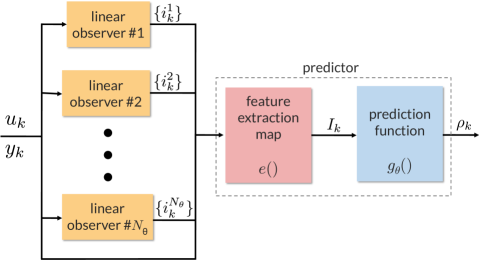
Figure 1: Virtual sensor architecture: bank of linear observers, feature extraction map $e$, and prediction function $g_{\theta}$.

We propose the following two alternatives for the FE map, namely

$$e^{\mathrm{FE}}_{\theta}({\mathcal{I}}_{k})=\{\hat{e}_{k}^{1},\hat{e}^{1}_{k-\ell},\ldots,\hat{e}^{N}_{k},\ldots,\hat{e}^{N}_{k-\ell},u_{k},y_{k}\}$$ (11a)

where $$\hat{e}_{m}^{j}\triangleq(\hat{y}^{j}_{m}-y_{m})$$ and, to further reduce the number of features, the more aggressive and higher compression FE map

$$e^{\mathrm{FE}}_{\theta}({\mathcal{I}}_{k})=\{\nu^{1}_{k},\dots,\nu^{N}_{k},u_{k},y_{k}\}$$ (11b)

where

$$\nu^{i}_{k}=\sum_{r=k-\ell}^{k}\sqrt{\frac{m(r-\ell)}{\ell}(\hat{y}^{i}_{r}-y_{r})^{\prime}(\hat{y}^{i}_{r}-y_{r})}$$

and $m:\mathbb{Z}\to\mathbb{R}$ is an appropriate weighting function.

The rationale for the maps in (11b) is that one of the most common features used in hypothesis testing algorithms is the estimate of the covariance of the residuals produced by each observer. Thus, this approach can be thus considered a generalization of the window-based hypothesis-testing algorithms explored in the literature, such as in [20, 31]. The FE map (11b) brings this idea one step further so that $e^{\mathrm{FE}}_{\theta}(\mathcal{I}_{k})$ has only $n_{I}=(N+1)n_{y}+n_{u}$ components. This means that the input to $g_{\theta}$, and therefore the predictor itself, can get very compact.

Note that both the window-size $\ell$ and the weighting function $m$ are hyper-parameters of the proposed approach. In particular, the value of $\ell$ must be chosen carefully: if it is too small the time window of past output prediction errors may not be long enough for a slow observer. On the other hand, if $\ell$ is too large the virtual sensor may become excessively slow in detecting changes of $\rho_{k}$. The weighting function $m$ acts in a similar manner and can be used for fine-tuning the behavior of the predictor.

Note also that our choices for $e^{\mathrm{FE}}_{\theta}$ in (11b) are not the only possible ones, nor necessarily the optimal ones. For example, by setting $e^{\mathrm{FE}}_{\theta}({\mathcal{I}}_{k})={\mathcal{I}}_{k}$, and therefore $f_{\theta}=g_{\theta}$, one recovers the general case in (9). Finally, note that our analysis has been restricted to a pre-assigned function $e^{\mathrm{FE}}$, although this could also be learned from data. To this end, the interested reader is referred to [11, 32, 33] and the references therein.

3.3.1 Choice of learning techniques

As highlighted in [34], in order to target an embedded implementation, it is necessary to envision a learning architecture for $g_{\theta}$ that has a limited memory footprint and requires a small and well predictable throughput. To do so, instead of developing an application-specific functional approximation scheme, we resort to well-understood machine-learning techniques. In particular, three possible options are explored in this work , all well suited for our purposes and which require a number of floating-point operations (flops) for their evaluation which is independent of the number of samples used in the training phase, in contrast for example to K-nearest neighbor regression [23].

Remark: Such choices are not the only possible ones and other approaches may be better suitable for specific needs. For example, if one is interested in getting an uncertainty measure coupled to the predictions, the use of regression techniques based on Gaussian processes [35] could be more suitable.

3.3.2 Compact artificial neural networks

Artificial neural networks (ANN) are a widely used machine-learning technique that has already shown its effectiveness in other MMAE-based schemes [36]. An option to make ANN very lightweight is to resort on very compact feed-forward topologies comprised of a small number of layers and a computationally cheap activation function in their hidden neurons [37], such as the Rectified Linear Unit (ReLU) [38]

$$f_{\rm ReLU}(x)=\max\{0,x\}$$ (12)

As we want to predict real-valued quantities, we consider a linear activation function for the output layer of the network.

3.3.3 Decision-tree and random-forest regression

DTRs of limited depth are in general extremely cheap to evaluate yet offer a good approximation power [39]. Other advantages of DTRs are that they can also work effectively with non-normalized data, they can be well interpreted [40], and the contribution provided by each input feature is easily recognizable. The main disadvantage of DTRs is instead that they can suffer from high variance. For this reason, in this work, we also explore the use of random-forest regressors (RFRs) [41], which try to solve the issue by bagging together multiple trees at the cost of both a more problematic interpretation and higher computational requirements.

3.4 Hyper-parameters and tuning procedures

The overall architecture of the proposed virtual sensor is shown in Figure 1. Its main hyper-parameters are:

1. the number $N_{\theta}$ of local models to learn from experimental data, related to the number of leaves of the DTR (see Section 3.1.1);

2. the order $M$ of the local models (see Section 3.1);

3. the window size $\ell$ of the predictor, which sets the number of past/current input features provided to the predictor at each time to produce the estimate $\hat{\rho}_{k}$ (see Section 3.3).

From a practical point of view, tuning $M$ is relatively easy, as one can use as the optimal cost reached by solving (5) an indirect performance indicator to properly trade-off between the quality of fit and storage constraints. Feature selection approaches such as the one presented in [42] can also be used. The window size $\ell$ of the predictor is also easily tunable by using any feature selection method compatible with the chosen regression technique. A more interesting problem is choosing the correct number of local models $N_{\theta}$, especially if one considers that MMAE-like schemes often do not perform well if too many models are considered [43]. Finally, we mention that the proposed method also requires defining the feature extraction map and the predictor structure.

As with most black-box approaches, and considering the very mild assumption we made on on the system $\Sigma_{P}$ that generates the data, the robustness of the virtual sensor with respect to noise and other sources of uncertainty can only be assessed a posteriori. For this reason, Section 4.2 below reports a thorough experimental analysis to assess such robustness properties.

4 Numerical results

In this section, we explore the performance of the proposed virtual sensor approach on a series of benchmark problems. All tests were performed on a PC equipped with an Intel Core i7 4770k CPU and 16 GB of RAM. The models introduced in this section were used only to generate the training datasets and to test the virtual sensor and are totally unknown to the learning method. We report such models to facilitate reproducing the numerical results reported in this section.

4.1 Learning setup

All the ANNs involved in learning the virtual sensors were developed in Python using the Keras framework [44] and are composed of 3 layers (2 ReLU layers with an equal number of neurons and an linear output layer), with overall $60$ hidden neurons. The ANNs are trained using the AMSgrad optimization algorithm [45]. During training, 5% of the training set is reserved to evaluate the stopping criteria.

Both DTR and RFR are trained using scikit-learn [46] and, in both cases, the max depth of the trees is capped to 15. RFRs consist of 10 base classifiers. The DTR used to extract the set of local models, as shown in Section 3.1.1, is instead constrained to have a maximum number of leaves equal to the number $N_{\theta}$ of linear models considered in each test. The loss function $L_{M_{LPV}}$ used is the well known mean absolute error [47]. In all other cases, the standard mean-squared error (MSE) [48] is considered.

The performance of the overall virtual sensor is assessed on the testing dataset in terms of the following fit ratio ($\mathrm{FIT}$) and normalized root mean-square error (NRMSE)

$$\mathrm{FIT}=\max\left\{0,1-\frac{\|\rho_{\mathcal{T}}-\hat{\rho}_{\mathcal{T}}\|_{2}}{\|\bar{\rho}-\rho_{\mathcal{T}}\|_{2}}\right\}$$ (13a)

$$\mathop{\rm NRMSE}\nolimits=\max\left\{0,1-\frac{\|\rho_{\mathcal{T}}-\hat{\rho}_{\mathcal{T}}\|_{2}}{\sqrt{\mathcal{T}}|\max(\rho_{\mathcal{T}})-\min(\rho_{\mathcal{T}})|}\right\}$$ (13b)

computed component-wise, where $\bar{\rho}$ is the mean value of the test sequence $\rho_{\mathcal{T}}=\{\rho_{i}\}_{i=1}^{\mathcal{T}}$ of the true values and $\hat{\rho}_{\mathcal{T}}$ is its estimate.

For each examined test case, we report the mean value and standard deviation of the two figures in (13b) over ten different runs, each one involving different realizations of all the excitation signals $u_{k}$, $p_{k}$, and measurement noise.

4.2 A synthetic benchmark system

We first explore the performance of the proposed approach and analyze the effect of its hyper-parameters on a synthetic multi-input single-output benchmark problem. Consider the nonlinear time-varying system

$$\Sigma_{\mathrm{S}}=\left\{\begin{array}[]{rcl}x_{k+1}&=&Hx_{k}+\frac{\alpha}{2}\mathop{\rm atan}\nolimits(x_{k})+\log(\rho_{k}+1)Fu_{k}\\ \rho_{k+1}&=&h(\rho_{k},u_{k},k)\\ y_{k}&=&-(1+e^{\rho_{k}})\left[\begin{array}[]{ccccc}0&0&0&0&1\end{array}\right]x_{k}\end{array}\right.$$ (14a)

where $$x\in\mathbb{R}^{5} \mathop{\rm atan}\nolimits \alpha,\rho_{k}\in\mathbb{R} H F$$, is the arc-tangent element-wise operator, , matrices and are defined as

$$\begin{array}[]{lr}H={\begin{bmatrix}0.0&0.1&0.0&0.0&0.0&\\ 0.0&0.0&-1.0&0.0&0.0&\\ 0.0&0.0&0.0&1.0&0.0&\\ 0.0&0.0&0.0&0.0&1.0&\\ -0.00909&0.0329&0.29013&-1.05376&1.69967\end{bmatrix}\vspace*{.5cm}}\\ F={\begin{bmatrix}-0.71985&-0.1985\\ 0.57661&0.917661\\ 1.68733&-0.68733\\ -2.14341&2.94341\\ 1.&1.\\ \end{bmatrix}\par}\end{array}$$ (14b)

and function $h$ is defined by

$$h(\rho_{k},u_{k},k) = \left\{\begin{array}[]{l}p_{k}~{}~{}\mbox{if~{}}~{}p_{k}\in[-0.95,0.95]\\ \frac{p_{k}}{2}~{}\mbox{otherwise}\end{array}\right.$$ (14e)

$$p_{k} = 0.999\rho_{k}+0.03\omega_{k},\quad\omega_{k}\sim\mathcal{N}(0,1)$$ (14f)

mimicking the phenomenon of a slow parameter drift. Unless otherwise stated, in the following we consider $\alpha=1$.

Training datasets of various sizes (up to $25,000$ samples) and a dataset of $5,000$ testing samples are generated by exciting the benchmark system (4.2) with a zero-mean white Gaussian noise input $u_{k}$ with unit standard deviation. All signals are then normalized using the empirical average and standard deviation computed on the training set and superimposed with a zero-mean white Gaussian noise with a standard deviation of $0.03$ to simulate measurement noise.

We consider local ARX linear models involving past $M=5$ inputs and outputs and solve Problem (5) via a fully connected feed-forward ANN. In the feature extraction process, we set the window $\ell=7$ on which the feature extraction process operates. In all tests we also assume $m(i)\equiv 1$, $\forall i\in\mathbb{Z}$. Unless otherwise noted, we consider deadbeat Luenberger observers, i.e., we place the observer poles in $z=0$ using the Scipy package [49].

4.3 Dependence on the number $N$ of samples

No. of acquired samples $N$	5000	15000	25000	5000	15000	25000
	FE map (11b)			FE map (11a)
average FIT (13a)	0.695	0.769	0.781	0.710	0.799	0.820
standard deviation	0.077	0.031	0.026	0.079	0.026	0.020
average NRMSE (13b)	0.934	0.951	0.953	0.937	0.957	0.961
standard deviation	0.017	0.004	0.002	0.017	0.003	0.002

Table 1: Accuracy of the virtual sensor using datasets of different size $K$.

We analyze the performance obtained by the synthesized virtual sensor with respect to the number $N$ of samples acquired for training during the experimental phase. Assessing the scalability of the approach with respect to the size of the dataset is extremely interesting because most machine learning techniques, and in particular neural networks, often require a large number of samples to be effectively trained.

Table 1 shows the results obtained by training the sensor with various dataset sizes when $N_{\theta}=5$ observers and an ANN predictor are used both using the proposed high-compression FE map (11b) and using the map in (11a). It is apparent that good results can already be obtained with 15,000 samples. With smaller datasets, fit performance instead remarkably degrades, especially when using the less aggressive FE map (11a).

4.4 Robustness toward measurement noise

We analyze next the performance of the proposed approach in the presence of various levels of measurement noise. In particular, we test the capabilities of the virtual sensor with $N_{\theta}=5$ deadbeat observers when trained and tested using data obtained from 14a and corrupted with a zero-mean additive Gaussian noise with different values of standard deviation $\sigma_{N}$. As in the other tests, noise is applied to the signal after normalization. The training dataset contains $25,000$ samples.

The results, reported in Table 2, show a very similar trend for all three functional approximation techniques and, in particular, a very steep drop in performance when moving from $\sigma_{N}=0.03$ to $\sigma_{N}=0.06$. This fact suggests that a good signal-to-noise ratio is necessary to achieve good performance with the proposed approach. This finding is not surprising, as our method is entirely data-driven, it has more difficulties in filtering noise out compared to model-based methods.

Performance of ANN, RFR, and DTR is similar to what observed in the previous tests.

Predictor		Standard deviation $\sigma_{N}$ of additive noise
		$0.01$	$0.03$	$0.06$
DTR		0.753 (0.024)	0.716 (0.033)	0.667 (0.046)
RFR		0.801 (0.021)	0.771 (0.027)	0.731 (0.039)
ANN		0.807 (0.020)	0.781 (0.026)	0.740 (0.036)

Table 2: Average FIT (13a) (standard deviation) for the three proposed learning architectures different sensor noise intensity.

4.5 Dependence on the prediction function

We analyze the difference in performance between the three proposed learning models for function $g_{\theta}$ when using $N_{\theta}=5$ linear models. The corresponding results are reported in Table 3, where it is apparent that as soon as enough samples are available, both RFRs and ANNs essentially perform the same, especially when using the more aggressive FE map (11b). For smaller training datasets, the ANN-based predictor performs slightly better, especially in terms of variance. Regression trees show worst performance but they are still able to produce acceptable estimates.

Regarding the results obtained using the FE map (11a), ANNs are remarkably more effective than the other two methods. In particular, while RFRs still show acceptable performance, DTRs fail almost completely.

Predictor	FE map	Number $N$ of acquired samples
		5000	15000	25000
DTR	(11b)	0.624 (0.094)	0.698 (0.042)	0.716 (0.033)
RFR		0.685 (0.104)	0.754 (0.034)	0.771 (0.027)
ANN		0.695 (0.077)	0.769 (0.031)	0.781 (0.026)
DTR	(11a)	0.412 (0.156)	0.589 (0.054)	0.646 (0.029)
RFR		0.596 (0.180)	0.743 (0.038)	0.768 (0.038)
ANN		0.710 (0.079)	0.799 (0.026)	0.820 (0.020)

Table 3: Average FIT (13a) (standard deviation) for the three proposed learning architectures for different numbers $K$ of samples in the training dataset.

4.6 Dependence on the observer dynamics

The dynamics of state-estimation errors heavily depend on the location of the observer poles set by the Luenberger observer (7), such as due to the chosen covariance matrices in the case stationary KFs are used for observer design. In this section, we analyze the sensitivity of the performance achieved by the virtual sensor with respect to the chosen settings of the observer.

Using $N_{\theta}=5$ models again, the Luenberger observers were tuned to have their poles all in the same location $z\in\mathbb{C}$ inside the unit disk and vary such a location in different tests. In addition, we also consider stationary Kalman filters designed assuming the following model

$$\left\{\begin{array}[]{rcl}\xi^{j}_{k+1}&=&A_{j}\xi_{k}+B_{j}u_{k}+d_{j}+w_{k}\\ y^{j}_{k}&=&C_{j}\xi_{k}+e_{j}+v_{k}\end{array}\right.$$ (15)

where $w_{k}\sim\mathcal{N}(0,I)$ and $v_{k}\sim\mathcal{N}(0,\lambda I)$ are uncorrelated white noise signals of appropriate dimensions and $\lambda\geq 0$.

The resulting virtual sensing performance figures are reported in Table 4 for a training dataset of $N=25,000$ samples and RFR-based prediction. While performance is satisfactory in all cases, fast observer poles allow better performance when pole placement is used. Nevertheless, in all but the deadbeat case, KFs provide better performance regardless of the chosen covariance term $\lambda$.

	pole placement			Kalman filter
observer settings	$z=0.0$	$z=0.4$	$z=0.8$	$\lambda=1$	$\lambda=10$	$\lambda=0.1$
average FIT (13a)	0.771	0.698	0.467	0.773	0.762	0.772
standard deviation	0.027	0.033	0.050	0.026	0.029	0.026
average NRMSE (13b)	0.951	0.935	0.886	0.951	0.949	0.951
standard deviation	0.002	0.004	0.006	0.002	0.003	0.002

Table 4: Average prediction performance with respect to observer settings.

4.7 Dependence on the number $N_{\theta}$ of local models

To explore how sensitive the virtual sensor is with respect to the number $N_{\theta}$ of local LTI model/observer pairs employed, we consider the performance obtained using $N_{\theta}=2,3,4,5,7$ local models on the 25,000 sample dataset. The results obtained using RFR based virtual sensors are reported in Table 5 and show that performance quickly degrades if too few local models are employed. At the same time, one can also note that a large number of models is not necessarily more effective. This finding suggests that the proposed virtual sensor can be easily tuned by increasing the number of models until the accuracy reaches a plateau.

Figure 2 shows the estimates of $\rho_{k}$ obtained by the virtual sensor for $N_{\theta}=5$, using deadbeat observers and a RFR predictor, for a given realization of (14f).

N	2	3	5	7
average FIT (13a)	0.685	0.766	0.771	0.777
standard deviation	0.035	0.027	0.027	0.028
average NRMSE (13b)	0.932	0.950	0.951	0.952
standard deviation	0.004	0.002	0.002	0.002

Table 5: Prediction performance of the virtual sensor with respect to the number $N_{\theta}$ of LTI models.

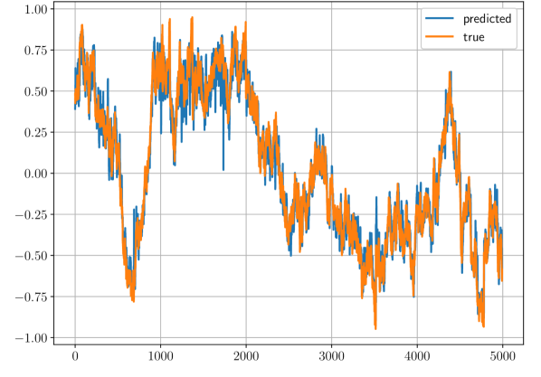
Figure 2: Example of reconstruction of $\rho_{k}$ by the virtual sensor based on $N_{\theta}=5$ local models, using deadbeat observers and a RFR predictor. The figure reports the actual value of $\rho_{k}$ (orange line) and its estimate $\hat{\rho}_{k}$ (blue line).

4.8 Dependence on the dynamics of $\rho_{k}$

Let us consider a different model than (14e)–(14f) to generate the value of $p_{k}$ that defines the signal $\rho_{k}$, namely the deterministic model

$$p_{k}=\cos\left(\frac{1}{\beta}k\right)$$ (16)

with $\beta=200$. In this way, it is possible to test the effectiveness of our approach in a purely parameter-varying setting and its robustness against discrepancies between the way training data and testing data are generated.

The results reported in Tables 6 and 7 are obtained by using $N_{\theta}=5$ models and 25,000 samples using all the three different prediction functions and deadbeat observers. While (16) is used to generate both training and testing data to produce the results shown in Table 6, Table 7 shows the case in which the training dataset is generated by (14e)–(14f) while the testing dataset by (16). It is apparent that the proposed approach is able to work effectively also in the investigated parameter-varying context in all cases and able to cope with sudden changes of $\rho_{k}$.

Predictor	DTR	RFR	ANN
average FIT (13a)	0.826	0.860	0.859
standard deviation	0.007	0.004	0.005
average NRMSE (13b)	0.948	0.958	0.957
standard deviation	0.002	0.001	0.001

Table 6: Average accuracy of the virtual sensor employing various kind of prediction functions when both training and testing data are generated by using (16).

predictor	DTR	RFR	ANN
average FIT (13a)	0.755	0.778	0.834
standard deviation	0.044	0.066	0.011
average NRMSE (13b)	0.925	0.932	0.949
standard deviation	0.014	0.020	0.003

Table 7: Average accuracy of the virtual sensor for different prediction functions with training data generated from (14f) and testing data from (16).

4.9 A mode observer for switching linear systems

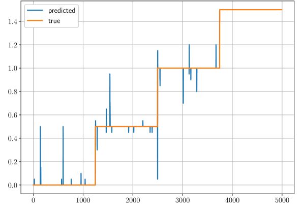
Figure 3: Mode reconstruction for switching linear systems (17): actual value of the mode $\rho_{k}$ (orange line) and its estimate $\hat{\rho}_{k}$ (blue line) provided by a RFR-based virtual sensor with a bank of 5 deadbeat observers.

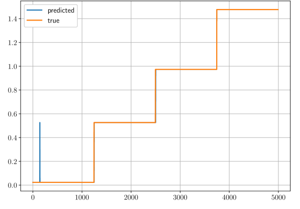
Figure 4: Mode reconstruction for switching linear systems (17): actual value of the mode $\rho_{k}$ (orange line) and its estimate $\hat{\rho}_{k}$ (blue line) provided by a RFC-based virtual sensor and 5 deadbeat observers.

An interesting class of systems which can be described by (1) are linear switching systems [50], a class of linear parameter varying systems in which $\rho_{k}$ can only assume a finite number $s$ of values $\rho^{1}$, $\ldots$, $\rho^{s}$. In this case, model (1) becomes the following discrete-time switching linear system

$$\Sigma\coloneqq\left\{\begin{array}[]{rcl}x_{k+1}&=&A_{\rho_{k}}x_{k}+B_{\rho_{k}}u_{k}\\ y_{k}&=&C_{\rho_{k}}x_{k}\end{array}\right.$$ (17)

For switching systems, the problem of estimating $\rho_{k}$ from input/output measurements is also known as the mode-reconstruction problem. In order to test our virtual sensor approach for mode reconstruction, we let the system generating the data be a switching linear system with $s=4$ modes obtained by the scheduling signal

$$\rho_{k}=\frac{1}{2}\left\lfloor\frac{4k}{N}\right\rfloor$$ (18)

where $N$ is the number of samples collected in the experiment and $\lfloor\cdot\rfloor$ is the downward rounding operator. For this test, the measurements about the mode acquired during the experiment are noise-free. As we are focusing on linear switching systems, we set $\alpha=0$.

As in Section 4.7, we test the performance of the RFR-based virtual sensor trained on 25,000 samples to reconstruct the value of $\rho_{k}$ when equipped with a different number $N_{\theta}$ of local models. The corresponding results are reported in Table 8 and show that the performance of the sensor again quickly saturates once the number of local models matches the actual number of switching modes.

$N_{\theta}$	2	3	4	5
average FIT (13a)	0.785	0.917	0.942	0.943
standard deviation	0.014	0.016	0.009	0.008
average NRMSE (13b)	0.920	0.969	0.979	0.979
standard deviation	0.005	0.006	0.003	0.003

Table 8: Accuracy of the virtual sensor employing different predictors for the switching linear system in (18).

The time evolution of the actual mode and the mode reconstructed by the virtual sensor is shown in Figure 3.

4.9.1 Performance obtained using a classifier in place of a regressor

The special case of mode reconstruction for switching systems can be also cast as a multi-category classification problem. Table 9 reports the F1-score [51] obtained by applying a virtual sensor based on a Random Forest Classifier (RFC) and 5 deadbeat observers to discern the current mode of the system. We consider only the case of samples correctly labeled, with the RFC subject to the same depth limitation of the non-categorical hypothesis tester. Table 9 also reports the classification accuracy of the non-categorical virtual sensor when coupled with a minimum-distance classifier (i.e., at each time $k$ the classifier will predict the mode $i$ associated with the value $\rho_{i}$ that is closest to $\hat{\rho}_{k}$). The results refer to a virtual sensor equipped with RFR and 5 deadbeat observers. It is interesting to note that the classifier architecture is also very effective with respect to the FIT metric (13a), achieving an average score of 0.945 with with a standard deviation of 0.010.

The time evolution of the actual mode and the mode reconstructed by the classifier-based virtual sensor is shown in Figure 4.

F1-score / mode #	1	2	3	4
RFC	0.997	0.994	0.996	0.998
standard deviation	0.001	0.002	0.002	0.001
RFR	0.996	0.995	0.995	0.997
standard deviation	0.002	0.002	0.002	0.002

Table 9: F1-score [51] obtained by the RFC-based virtual sensor (RFC) and by the RFR-based virtual sensor + minimum-distance classifier (RFR) on the 4-mode switching linear system (18) over 10 runs.

4.10 Nonlinear state estimation

This sections compares the proposed approach with standard model-based nonlinear state-estimation techniques on the problem of estimating the state of charge (SoC) of a lithium-ion battery, using the model proposed in [52].

In [52], the battery is modeled as the following nonlinear third-order dynamical system

$$\Sigma_{\mathrm{Battery}}=\left\{\begin{array}[]{l}\dot{x}_{1}(t)=\displaystyle{\frac{\scalebox{0.75}[1.0]{$-$}i(t)}{C_{c}}}\\ \dot{x}_{2}(t)=\displaystyle{\frac{\scalebox{0.75}[1.0]{$-$}x_{2}(t)}{R_{ts}(x_{1}(t))C_{ts}(x_{1}(t))}+\frac{i(t)}{C_{ts}(x_{1}(t))}}\\ \dot{x}_{3}(t)=\displaystyle{\frac{\scalebox{0.75}[1.0]{$-$}x_{3}(t)}{R_{tl}(x_{1}(t))C_{tl}(x_{1}(t))}+\frac{i(t)}{C_{ts}(x_{1}(t))}}\\ y(t)=E_{0}(x_{1}(t))-x_{2}(t)-x_{3}(t)-i(t)R_{s}(x_{1}(t))\end{array}\right.$$ (19)

where $x_{1}(t)$ is the SoC (pure number $\in[0,1]$ representing the fraction of the battery rated capacity that is available [53]), $y(t)$ [V] the voltage at the terminal of the battery, $i(t)$ [A] the current flowing through the battery,

$$\begin{array}[]{l}E_{0}(x_{1})=-a_{1}e^{-a_{x}x_{1}}+a_{3}+a_{4}x_{1}-a_{5}x_{1}^{2}+a_{6}x_{1}^{3}\\ R_{ts}(x_{1})=a_{7}e^{-a_{8}x_{1}}+a_{9}\\ R_{tl}(x_{1})=a_{10}e^{-a_{11}x_{1}}+a_{12}\\ C_{ts}(x_{1})=a_{13}e^{-a_{17}x_{1}}+a_{18}\\ R_{s}(x_{1})=a_{19}e^{-a_{20}x_{1}}+a_{21}\end{array}$$

and the values of the coefficients $a_{ij}$ correspond to the estimated values reported in Tables 1, 2, 3 of [52].

We analyze the capability of the proposed synthesis method of virtual sensors to reconstruct the value $\rho=x_{1}$ in comparison to a standard extended Kalman filter (EKF) [54] based on model (19) and assuming the process noise vector $w_{k}\in\mathbb{R}^{3}$ entering the state equation, $w_{k}\sim\mathcal{N}(0,Q)$, and measurement noise $v_{k}\perp w_{k}\sim\mathcal{N}(0,R)$ on the output $y$ for various realization of $R\in\mathbb{R}^{3\times 3},Q\in\mathbb{R}$. Model (19) is integrated by using an explicit Runge-Kutta 4 scheme.

The simulated system is sampled at the frequency $f_{s}=\frac{1}{5}$ Hz, starting from a fully charged state $x(0)=[1,~{}0,~{}0]^{\prime}$ and excited with a variable-step current signal $i(t)$ with constant amplitude

$$i(t)=\frac{1}{5}\max\left\{0,\cos\left(\frac{k}{100}\right)+\cos\left(\frac{k}{37}\right)\right\}+u_{k}$$ (20)

during the $k$-th sampling steps, with $u_{k}$ drawn from the uniform distribution $\mathcal{U}(0,0.4)$.

As the battery will eventually fully discharge, every time the SoC falls below the value $0.05$ the whole state is reset to the initial condition $x(0)$. The signals $y(t)$ and $i(t)$, once normalized, are processed as described in Section 4.1.

For this benchmark, an ANN-based virtual sensor with $N_{\theta}=5$ local linear models is selected. The corresponding KFs are also designed as described in Section 4.6 with $\lambda=0.1$, and FE map (11b). Training is performed over 25,000 samples.

The results obtained by the virtual sensor and EKFs designed with different values of the covariance matrices $Q,R$ of process and measurement noise, respectively, are reported in Figure 5. While EKF is, in general, more effective in tracking and denoising the true value of the SoC, it performs poorly in terms of bandwidth compared to the proposed virtual sensor, whose performance in terms of filtering noise out remains anyway acceptable. While both techniques are successful in estimating the SoC of the battery, we remark a main difference between them: EKF requires a nonlinear model of the battery, the virtual sensor does not.

Figure 5: Estimation of the SoC of the battery: true value $\rho_{k}$ (orange line), value $\hat{\rho}_{k}$ estimated by the virtual sensor (blue line), values $\hat{\rho}_{k}$ estimated by EKF for different settings of Q and R (green, red, violet, and brown lines).

4.11 Computation complexity of the prediction functions

The ANNs used in our tests require approximately between 1,000 and 3,000 weights to be fully parameterized. While this number is fixed by the network topology and depends on the number of inputs to the network, regularization techniques such as $\ell_{1}$-norm sparsifiers could be used here to reduce the number of nonzero weights (see for instance [55] and the reference therein), so to further reduce memory footprint.

Regarding the tree-based approaches, practical storage requirements are strongly influenced by the specific implementation and, in general, less predictable in advance due to their non-parametric nature. In any case, evaluating the predictors on the entire 5,000 sample test set on the reference machine only requires a few milliseconds, which makes the approach amenable for implementation in most modern embedded platforms.

The training procedure for all the proposed architectures is similarly affordable: on the reference machine, the whole training process is carried out in a few tens of seconds for a training set of 25,000 samples with negligible RAM occupancy.

5 Conclusions

This paper has proposed a data-driven virtual sensor synthesis approach, inspired by the MMAE framework, for reconstructing normally unmeasurable quantities such as scheduling parameters in parameter-varying systems, hidden modes in switching systems, and states of nonlinear systems.

The key idea is to use past input and output data (obtained when such quantities were directly measurable) to synthesize a bank of linear observers and use them as a base for feature-extraction maps that greatly simplify the learning process of the hypothesis testing algorithm that estimates said parameters. Thanks to its low memory and CPU requirements, the overall architecture is particularly suitable for embedded and fast-sampling applications.

Acknowledgments

This paper was partially supported by the Italian Ministry of University and Research under the PRIN’17 project “Data-driven learning of constrained control systems” , contract no. 2017J89ARP.

References

- [1] F.-R. López-Estrada, D. Rotondo, G. Valencia-Palomo, A review of convex approaches for control, observation and safety of linear parameter varying and Takagi-Sugeno systems, Processes 7 (11) (2019) 814.
- [2] R. Tóth, Modeling and Identification of Linear Parameter-Varying Systems, Springer, Berlin, Heidelberg, 2010.
- [3] F. D. Torrisi, A. Bemporad, HYSDEL — A tool for generating computational hybrid models, IEEE Trans. Contr. Systems Technology 12 (2) (2004) 235–249.
- [4] D. Rotondo, V. Puig, J. Acevedo Valle, F. Nejjari, FTC of LPV systems using a bank of virtual sensors: Application to wind turbines, in: Proc. of Conf. on Control and Fault-Tolerant Systems, 2013, pp. 492–497.
- [5] M. Witczak, Fault diagnosis and fault-tolerant control strategies for non-linear systems, Vol. 266, Springer, 2014.
- [6] J. Guzman, F.-R. López-Estrada, V. Estrada-Manzo, G. Valencia-Palomo, Actuator fault estimation based on a proportional-integral observer with nonquadratic Lyapunov functions, International Journal of Systems Science (2021) 1–14.
- [7] J.-J. Slotine, W. Li, Applied Nonlinear Control, Prentice Hall Englewood Cliffs, NJ, 1991.
- [8] M. Misin, V. Puig, LPV MPC control of an autonomous aerial vehicle, in: 2020 28th Mediterranean Conference on Control and Automation (MED), IEEE, 2020, pp. 109–114.
- [9] M.-H. Do, D. Koenig, D. Theilliol, observer design for singular nonlinear parameter-varying system, in: 2020 59th IEEE Conference on Decision and Control (CDC), IEEE, 2020, pp. 3927–3932.
- [10] K. J. Keesman, System identification: an introduction, Springer, 2011.
- [11] D. Masti, A. Bemporad, Learning nonlinear state-space models using deep autoencoders, in: Proc. 57th IEEE Conf. on Decision and Control, Miami Beach, FL, USA, 2018, pp. 3862–3867.
- [12] M. Milanese, C. Novara, K. Hsu, K. Poolla, The filter design from data (FD2) problem: Nonlinear set membership approach, Automatica 45 (10) (2009) 2350–2357.
- [13] T. Poggi, M. Rubagotti, A. Bemporad, M. Storace, High-speed piecewise affine virtual sensors, IEEE Transactions on Industrial Electronics 59 (2) (2012) 1228–1237.
- [14] E. Marchi, F. Vesperini, F. Eyben, S. Squartini, B. Schuller, A novel approach for automatic acoustic novelty detection using a denoising autoencoder with bidirectional LSTM neural networks, in: 2015 IEEE International Conference on Acoustics, Speech and Signal Processing (ICASSP), IEEE, 2015, pp. 1996–2000.
- [15] S. Aghabozorgi, A. S. Shirkhorshidi, T. Y. Wah, Time-series clustering–A decade review, Information Systems 53 (2015) 16–38.
- [16] M. D. Morse, J. M. Patel, An efficient and accurate method for evaluating time series similarity, in: Proceedings of the 2007 ACM SIGMOD international conference on Management of data, ACM, 2007, pp. 569–580.
- [17] A. Akca, M. Ö. Efe, Multiple model Kalman and particle filters and applications: a survey, IFAC-PapersOnLine 52 (3) (2019) 73–78.
- [18] D. Masti, D. Bernardini, A. Bemporad, Learning virtual sensors for estimating the scheduling signal of parameter-varying systems, in: 27th Mediterranean Conference on Control and Automation (MED), IEEE, Akko, Israel, 2019, pp. 232–237.
- [19] Y. Bar-Shalom, X. R. Li, T. Kirubarajan, Estimation with applications to tracking and navigation: theory algorithms and software, John Wiley & Sons, 2004.
- [20] B. N. Alsuwaidan, J. L. Crassidis, Y. Cheng, Generalized multiple-model adaptive estimation using an autocorrelation approach, IEEE Transactions on Aerospace and Electronic systems 47 (3) (2011) 2138–2152.
- [21] X.-R. Li, Y. Bar-Shalom, Multiple-model estimation with variable structure, IEEE Transactions on Automatic control 41 (4) (1996) 478–493.
- [22] L. Ljung, System identification: theory for the user, Prentice-Hall, 1987.
- [23] T. Hastie, R. Tibshirani, J. Friedman, The elements of statistical learning: prediction, inference and data mining, Springer-Verlag, New York, 2009.
- [24] G. E. Hinton, R. R. Salakhutdinov, Reducing the dimensionality of data with neural networks, Science 313 (5786) (2006) 504–507.
- [25] J. Feng, Z.-H. Zhou, Autoencoder by forest, in: Proceedings of the AAAI conference on artificial intelligence, Vol. 32, 2018.
- [26] S. Lloyd, Least squares quantization in PCM, IEEE Transactions on Information Theory 28 (2) (1982) 129–137.
- [27] A. Bemporad, V. Breschi, D. Piga, S. P. Boyd, Fitting jump models, Automatica 96 (2018) 11–21.
- [28] P. Mellodge, A Practical Approach to Dynamical Systems for Engineers, Woodhead Publishing, 2015.
- [29] S. M. Shinners, Modern Control System Theory and Design, 2nd Edition, John Wiley & Sons, Inc., New York, NY, USA, 1998.
- [30] C. Sammut, G. I. Webb (Eds.), Generative and Discriminative Learning, Springer US, 2010, pp. 454–455.
- [31] P. D. Hanlon, P. S. Maybeck, Multiple-model adaptive estimation using a residual correlation kalman filter bank, IEEE Transactions on Aerospace and Electronic Systems 36 (2) (2000) 393–406.
- [32] Y. Gao, L. Zhu, H.-D. Zhu, Y. Gan, L. Shang, Extract features using stacked denoised autoencoder, in: Intelligent Computing in Bioinformatics, Springer International Publishing, 2014, pp. 10–14.
- [33] I. Guyon, A. Elisseeff, An introduction to feature extraction, in: Feature extraction, Springer, 2006, pp. 1–25.
- [34] D. Masti, A. Bemporad, Learning binary warm starts for multiparametric mixed-integer quadratic programming, in: Proc. of European Control Conference, Naples, Italy, 2019, pp. 1494–1499.
- [35] C. E. Rasmussen, Gaussian processes in machine learning, in: Summer school on machine learning, Springer, 2003, pp. 63–71.
- [36] T. L. Vincent, C. Galarza, P. P. Khargonekar, Adaptive estimation using multiple models and neural networks, IFAC Proceedings Volumes 31 (29) (1998) 149–154.
- [37] B. Karg, S. Lucia, Efficient representation and approximation of model predictive control laws via deep learning, IEEE Transactions on Cybernetics 50 (9) (2020) 3866–3878.
- [38] V. Nair, G. E. Hinton, Rectified linear units improve restricted Boltzmann machines, in: International Conference on Machine Learning (ICML), 2010, pp. 807–814.
- [39] D. Masti, T. Pippia, A. Bemporad, B. De Schutter, Learning approximate semi-explicit hybrid mpc with an application to microgrids, in: 2020 IFAC World Congress, 2020.
- [40] R. L. Marchese Robinson, A. Palczewska, J. Palczewski, N. Kidley, Comparison of the predictive performance and interpretability of random forest and linear models on benchmark data sets, Journal of Chemical Information and Modeling 57 (8) (2017) 1773–1792.
- [41] L. Breiman, J. Friedman, C. J. Stone, R. Olshen, Classification and Regression Trees, CRC Press, 1984.
- [42] V. Breschi, M. Mejari, Shrinkage strategies for structure selection and identification of piecewise affine models, in: 2020 59th IEEE Conference on Decision and Control (CDC), IEEE, 2020, pp. 1626–1631.
- [43] X. R. Li, X. Zwi, Y. Zwang, Multiple-model estimation with variable structure. iii. model-group switching algorithm, IEEE Transactions on Aerospace and Electronic Systems 35 (1) (1999) 225–241.
- [44] F. Chollet, et al., Keras, https://keras.io (2015).
- [45] S. K. Sashank J. Reddi, Satyen Kale, On the convergence of Adam and beyond, Internation Conference on Learning Representations (2018).
- [46] L. Buitinck, G. Louppe, M. Blondel, F. Pedregosa, A. Mueller, O. Grisel, V. Niculae, P. Prettenhofer, A. Gramfort, J. Grobler, R. Layton, J. VanderPlas, A. Joly, B. Holt, G. Varoquaux, API design for machine learning software: experiences from the scikit-learn project, in: ECML PKDD Workshop: Languages for Data Mining and Machine Learning, 2013, pp. 108–122.
- [47] C. Sammut, G. I. Webb (Eds.), Mean Absolute Error, Springer US, Boston, MA, 2010, pp. 652–652.
- [48] C. Sammut, G. I. Webb (Eds.), Mean Squared Error, Springer US, Boston, MA, 2010, pp. 653–653.
- [49] E. Jones, T. Oliphant, P. Peterson, et al., SciPy: Open source scientific tools for Python, http://www.scipy.org/ (2001).
- [50] D. Liberzon, Switching in systems and control, Springer Science & Business Media, 2003.
- [51] Y. Sasaki, et al., The truth of the F-measure, Teach Tutor mater 1 (5) (2007) 1–5.
- [52] D. Ali, S. Mukhopadhyay, H. Rehman, A. Khurram, UAS based Li-ion battery model parameters estimation, Control Engineering Practice 66 (2017) 126–145.
- [53] H. Abdi, B. Mohammadi-ivatloo, S. Javadi, A. R. Khodaei, E. Dehnavi, Energy storage systems, in: G. Gharehpetian, S. M. Mousavi Agah (Eds.), Distributed Generation Systems, Butterworth-Heinemann, 2017, pp. 333–368.
- [54] B. D. O. Anderson, J. B. Moore, Optimal Filtering, Prentice-Hall, Englewood Cliffs, NJ, 1979.
- [55] I. Goodfellow, Y. Bengio, A. Courville, Regularization for deep learning, in: Deep Learning, MIT Press, 2016, http://www.deeplearningbook.org.