HADAD: A Lightweight Approach for Optimizing Hybrid Complex Analytics Queries (Extended Version)

Abstract.

Hybrid complex analytics workloads typically include $(i)$ data management tasks (joins, selections, etc. ), easily expressed using relational algebra (RA)-based languages, and $(ii)$ complex analytics tasks (regressions, matrix decompositions, etc.), mostly expressed in linear algebra (LA) expressions. Such workloads are common in many application areas, including scientific computing, web analytics, and business recommendation. Existing solutions for evaluating hybrid analytical tasks – ranging from LA-oriented systems, to relational systems (extended to handle LA operations), to hybrid systems – either optimize data management and complex tasks separately, exploit RA properties only while leaving LA-specific optimization opportunities unexploited, or focus heavily on physical optimization, leaving semantic query optimization opportunities unexplored. Additionally, they are not able to exploit precomputed (materialized) results to avoid recomputing (part of) a given mixed (RA and/or LA) computation.

In this paper, we take a major step towards filling this gap by proposing HADAD, an extensible lightweight approach for optimizing hybrid complex analytics queries, based on a common abstraction that facilitates unified reasoning: a relational model endowed with integrity constraints. Our solution can be naturally and portably applied on top of pure LA and hybrid RA-LA platforms without modifying their internals. An extensive empirical evaluation shows that HADAD yields significant performance gains on diverse workloads, ranging from LA-centered to hybrid.

1. Introduction

Modern analytical tasks typically include $(i)$ data management tasks (e.g., joins, filters) to perform pre-processing steps, including feature selection, transformation, and engineering (sculley2015hidden, ; kumar2016model, ; bose2017probabilistic, ; sparks2015automating, ; baylor2017tfx, ), tasks that are easily expressed using RA-based languages, as well as $(ii)$ complex analytics tasks (e.g., regressions, matrices decompositions), which are mostly expressed using LA operations  (kumar2017data, ). To perform such analytical tasks, data scientists can choose from a variety of systems, tools, and languages. Languages/libraries such as R (R, ) and NumPy (NumPy, ), as well as LA systems such as SystemML (boehm2016systemml, ), TensorFlow (abadi2016tensorflow, ) and MLlib  (sparkmlib, ) treat matrices and LA operations as first-class citizens: they offer a rich set of built-in LA operations. However, it can be difficult to express pre-processing tasks in these systems. Further, expression rewrites, based on equivalences that hold due to well-known LA properties, are not exploited in some of these systems, leading to missed optimization opportunities.

Many works propose integrating RA and LA processing , where both algebraic styles can be used together (luo2018scalable, ; chen2017towards, ; montdb, ; kernert2013bringing, ; kunft2019intermediate, ; spores, ; boehm2018optimizing, ).  (montdb, ) offers calling LA packages through user defined functions (UDFs), where libraries such as NumPy are embedded in the host language. Others suggest to extend RDBMS to treat LA objects as first-class citizens by using built-in functions to express LA operations (luo2018scalable, ; kernert2013bringing, ). However, LA operations’ semantics remain hidden behind these functions, where the optimizers treat as black-boxes. SPORES (spores, ) and SPOOF (boehm2018optimizing, ) optimize LA expressions by converting them into RA, optimizing the latter, and then converting the result back to an (optimized) LA expression. They only focus on optimizing LA pipelines containing operations that can be expressed in RA. The restriction is that LA properties of complex operations such as inverse, matrix-decompositions are entirely unexploited. Morpheus  (chen2017towards, ) speeds up LA pipelines over large joins by pushing computation into each joined table, thereby avoiding expensive materialization. LARA (kunft2019intermediate, ) focuses on low-level optimization by exploiting data layouts (e.g., column-wise) to choose LA operators’ physical implementations. A limitation of such approaches is that they lack high-level reasoning about LA properties and rewrites, which can drastically enhance the pipelines’ performance (thomas2018comparative, ).

Further, aforementioned solutions do not support semantic query optimization, which includes exploiting integrity constraints and materialized views and can bring enormous performance advantages in hybrid RA-LA and even plain LA settings.

We propose HADAD, an extensible lightweight framework for providing semantic query optimization (including views-based, integrity constraint-based, and LA property-based rewriting) on top of both pure LA and hybrid RA-LA platforms, with no need to modify their internals. At the core of HADAD lies a common abstraction: relational model with integrity constraints, which enables reasoning in hybrid settings. Moreover, it makes it very easy to extend HADAD’s semantic knowledge of LA operations by simply declaring appropriate constraints, with no need to change HADAD code. As we show, constraints are sufficiently expressive to declare (and thus allow HADAD to exploit) more properties of LA operations than previous work could consider.

Last but not least, our holistic, cost-based approach enables to judiciously apply for each query the best available optimization. For instance, given the computation $M(NP)$ for some matrices $M$, $N$ and $P$, we may rewrite it into $(MN)P$ if its estimated cost is smaller than that of the original expression, or we may turn it into $MV$ if a materialized view $V$ stores exactly the result of $(NP)$.

HADAD capitalizes on a framework previously introduced in (estocada-sigmod, ) for rewriting queries across many data models, using materialized views, in a polystore setting that does not include the LA model. The novelty of HADAD is to extend the benefits of rewriting and views optimizations to pure LA and hybrid RA-LA computations, which are crucial for ML workloads.

Contributions. The paper makes the following contributions:

1. We propose an extensible lightweight approach to optimize hybrid complex analytics queries. Our approach can be implemented on top of existing systems without modifying their internals; it is based on a powerful intermediate abstraction that supports reasoning in hybrid settings, namely a relational model with integrity constraints.

2. We formalize the problem of rewriting computations using previously materialized views in hybrid settings. To the best of our knowledge, ours is the first work that brings views-based rewriting under integrity constraints in the context of LA-based pipelines and hybrid analytical queries.

3. We provide formal guarantees for our solution in terms of soundness and completeness.

4. We conduct an extensive set of empirical experiments on typical LA- and hybrid-based expressions, which show the benefits of HADAD.

Outline. The rest of this paper is organized as follows: §2 highlights HADAD’s optimizations that go beyond the state of the art based on real-world scenarios, §3 formalizes the query optimization problem in the context of a hybrid setting. §5 provides an end-to-end overview of our approach. §6 presents our novel reduction of the rewriting problem into one that can be solved by existing techniques from the relational setting. §7 describes our extension to the query rewriting engine, integrating two different cost models, to help prune out inefficient rewritings as soon as they are enumerated. We formalize our solution’s guarantees in §8 and present the experiments in §9. We discuss related work and conclude in §10.

2. HADAD Optimizations

We highlight below examples of performance-enhancing opportunities that are exploited by HADAD and not being addressed by LA-oriented and cross RA-LA existing solutions.

LA Pipeline Optimization. Consider the Ordinary Least Squares Regression (OLS) pipeline: $(X^{T}X)^{-1}(X^{T}y)$, where $X$ is a square matrix of size 10K$\times$10K and $y$ is a vector of size 10K$\times$1. Suppose available a materialized view $V=X^{-1}$. HADAD rewrites the pipeline to $(V(V^{T}(X^{T}y))$, by exploiting the LA properties $(CD)^{-1}=D^{-1}C^{-1}$, $(CD)E=C(DE)$ and $(D^{T})^{-1}=(D^{-1})^{T}$ as well as the view $V$. The rewriting is more efficient than the original pipeline since it avoids computing the expensive inverse operation. Moreover, it optimizes the matrix chain multiplication order to minimize the intermediate result size. This leads to a 150$\times$ speed-up on MLlib (meng2016mllib, ). Current popular LA-oriented systems  (R, ; NumPy, ; boehm2016systemml, ; abadi2016tensorflow, ; meng2016mllib, ) are not capable of exploiting such rewrites, due to the lack of systematic exploration of standard LA properties and views.

Hybrid RA-LA Optimization. Cross RA-LA platforms such as Morpheus (chen2017towards, ), SparkSQL (armbrust2015spark, ) and others (kunft2019intermediate, ; aranasosIPSPPX20, ) can greatly benefit from HADAD’s cross-model optimizations, which can find rewrites that they miss.

Factorization of LA Operations over Joins. For instance, Morpheus implements a powerful optimization that factorizes an LA operation on a matrix M obtained by joining tables R and S and casting the join result as a matrix. Factorization pushes the LA operation on M to operate on R and S, cast as matrices.

Consider a specific instantiation of factorization: colSums(MN), where matrix M has size 20M$\times$ 120 and N has size 120$\times$100; both matrices are dense. The colSums operation sums up the elements in each column, returning the vector of these sums (the operation is common in ML algorithms such as K-means clustering  (macqueen1967some, )). On this pipeline, Morpheus applies a multiplication factorization rule to push the multiplication by N down to R and S: it computes RN and SN, then concatenates the resulting matrices to obtain MN. The size of this intermediate result is 20M$\times$100. Finally, colSums is applied to the intermediate result, reducing to a 1$\times$100 vector.

HADAD can help Morpheus do much better, by pushing the colSums operator to R and S (instead of the multiplication with N), then concatenating the resulting vectors. This leads to much smaller intermediate results, since the combined size of vectors colSums$($R$)$ and colSums$($S$)$ is only 1$\times$120.

To this end, HADAD rewrites the pipeline to colSums(M)N by exploiting the property colSums$(AB)\ =$colSums$(A)B$ and applying its cost estimator, which favors rewritings with a small intermediate result size. Evaluating this HADAD-produced rewriting, Morpheus’s multiplication pushdown rule no longer applies, while the colSums pushdown rule is now enabled, leading to 125$\times$ speed-up.

Pushing Selection from LA Analysis to RA Preprocessing. Consider another hybrid example on a Twitter dataset  (twitter, ). The JSON dataset contains tweet ids, extended tweets, entities including hashtags, filter-level, of media, URL, and tweet text, etc. We implemented it on SparkSQL (with SystemML (boehm2016systemml, )).

In the preprocessing stage, our SparkSQL query constructs a tweet-hashtag filter-level matrix N of size 2M$\times$1000, for all tweets posted from “USA” mentioning “covid”, where rows are tweets, columns are hashtags, and values are filter-levels..

N is then loaded into SystemML, where rows with filter-level less than 4 are selected. The result undergoes an Alternating Least Square (ALS)  (Mitchell97, ) computation. A core building block of the ALS computation is the LA pipeline $(uv^{T}-$ N$)v$. In our example, $u$ is a tweet feature vector (of size 2M$\times$1) and $v$ is a hashtag feature vector (of size 1000$\times$1).

We have two materialized views available: $V_{1}$ stores the tweet id and text as a text datasource in Solr, and $V_{2}$ stores tweet id, hashtag id, and filter-level for all tweets posted from “USA”, and is materialized on disk as CSV file. The rewriting modifies the preprocessing of N by introducing $V_{1}$ and $V_{2}$; it also pushes the filter-level selection from the LA pipeline into the preprocessing stage. To this end, it rewrites $(uv^{T}-$ N$)v$ to $uv^{T}v-$N$v$, which is more efficient for two reasons. First, N is ultra sparse (0.00018% non-zero), which renders the computation of N$v$ extremely efficient. Second, SystemML evaluates the chain $uv^{T}v$ efficiently, computing $v^{T}v$ first, which results in a scalar, instead of computing $uv^{T}$, which results in a dense matrix of size 2M$\times$1000 (HADAD’s cost model realizes this). Without the rewriting help from HADAD, SystemML is unable to exploit its own efficient operations for lack of awareness of the distributivity property of vector multiplication over matrix addition, $Av+Bv=(A+B)v$. The rewriting achieves 14$\times$ speed-up.

HADAD detects and applies all the above-mentioned optimizations combined. It captures RA-, LA-, and cross-model optimizations precisely because it reduces all rewrites to a single setting in which they can synergize: relational rewrites under integrity constraints.

3. Problem Statement

We consider a set of value domains $\mathcal{D}_{i}$, e.g., $\mathcal{D}_{1}$ denotes integers, $\mathcal{D}_{2}$ denotes real numbers, $\mathcal{D}_{3}$ strings, etc, and two basic data types: relations (sets of tuples) and matrices (bi-dimensional arrays). Any attribute in a tuple or cell in a matrix is a value from some $\mathcal{D}_{i}$. We assume a matrix can be implicitly converted into a relation (the order among matrix rows is lost), and the opposite conversion (each tuple becomes a matrix line, in some order that is unknown, unless the relation was explicitly sorted before the conversion).

We consider a hybrid language $\bm{\mathcal{L}}$, comprising a set $R_{ops}$ of (unary or binary) RA operators; concretely, $R_{ops}$ comprises the standard relational selection, projection, and join. We also consider a set $L_{ops}$ of LA operators, comprising: unary (e.g., inversion and transposition) and binary (e.g., matrix product) operators The full set $L_{ops}$ of LA operations we support is detailed in §6.1. A hybrid expression in $\bm{\mathcal{L}}$ is defined as follows:

• any value from a domain $\mathcal{D}_{i}$, any matrix, and any relation, is an expression;

• (RA operators): given some expressions $E,E^{\prime}$, $ro_{1}(E)$ is also an expression, where $ro_{1}\in R_{ops}$ is a unary relational operator, and $E$’s type matches $ro_{1}$’s expected input type. The same holds for $ro_{2}(E,E^{\prime})$, where $ro_{2}\in R_{ops}$ is a binary relational operator (i.e., the join);

• (LA operators): given some expressions $E,E^{\prime}$ which are either numeric matrices or numbers (which can be seen as degenerate matrices of $1\times 1$), and some real number $r$, the following are also expressions: $lo_{1}(E)$ where $lo_{1}\in L_{ops}$ is a unary operator, and $lo_{2}(E,E^{\prime})$ where $lo_{2}\in L_{ops}$ is a binary operator (again, provided that $E,E^{\prime}$ match the expected input types of the operators).

Clearly, an important set of equivalence rules hold over our hybrid expressions, well-known respectively in the RA and the LA literature. These equivalences lead to alternative evaluation strategies for each expression. Further, we assume given a (possibly empty) set of materialized views $\bm{\mathcal{V}}\in\bm{\mathcal{L}}$, which have been previously computed over some inputs (matrices and/or relations), and whose results are directly available (e.g., as a file on disk). Detecting when a materialized view can be used instead of evaluating (part of) an expression is another important source of alternative evaluation strategies.

Given an expression $E$ and a cost model that assigns a cost (a real number) to an expression, we consider the problem of identifying the most efficient rewrite derived from $E$ by: ($i$) exploiting RA and LA equivalence rules, and/or ($ii$) replacing part of an expression with a scan of a materialized view equivalent to that expression.

Below, we detail our approach, the equivalence rules we capture, and two alternative cost models we devised for this hybrid setting. Importantly, our solution (based on a relational encoding with integrity constraints) capitalizes on the framework previously introduced in (estocada-sigmod, ), where it was used to rewrite queries using materialized views in a polystore setting, where the data, views, and query cover a variety of data models (relational, JSON, XML, etc. ). Those queries can be expressed in a combination of query languages, including SQL, JSON query languages, XQuery, etc. The ability to rewrite such queries using heterogeneous views directly and fully transfers to HADAD: thus, instead of a relation, we could have the (tuple-structured) results of an XML or JSON query; views materialized by joining an XML document with a JSON one and a relational database could also be reused. The novelty of our work is to extend the benefits of rewriting and view-based optimization to LA computations, crucial for ML workloads. In §6, we focus on capturing matrix data and LA computations in the relational framework, along with relational data naturally; this enables our novel, holistic optimization of hybrid expressions.

4. PRELIMINARIES

We recall conjunctive queries (chandra1977optimal, ), integrity constraints (AHV95, ), and query rewriting under constraints (pacb-paper, ); these concepts are at the core of our approach.

4.1. Conjunctive Query and Constraints

A conjunctive query (or simply CQ) $\mathcal{Q}$ is an expression of the form $\mathcal{Q}(\overline{x})\mbox{:- }R_{1}(\overline{y}_{1}),\dots,R_{n}(\overline{y}_{n})$, where each $R_{i}$ is a predicate (relation) of some finite arity, and $\overline{x},\overline{y}_{1},\dots,\overline{y}_{n}$ are tuples of variables or constants. Each $R_{i}(\overline{y}_{i})$ is called a relational atom. The expression $\mathcal{Q}(\overline{x})$ is the head of the query, while the conjunction of relational atoms $R_{1}(\overline{y}_{1}),\dots,R_{n}(\overline{y}_{n})$ is its body. All variables in the head are called distinguished. Also, every variable in $\overline{x}$ must appear at least once in $\overline{y}_{1},\dots,\overline{y}_{n}$. Different forms of constraints have been studied in the literature (AHV95, ). In this work, we use Tuple Generating Dependencies (TGDs) and Equality Generating Dependencies (EGDs), stated by formulas of the form $\forall x_{1},\dots x_{n}$ $\phi(x_{1},\dots x_{n})\rightarrow\exists z_{1},\dots,z_{k}$ $\psi(y_{1},\dots,y_{m})$, where $\{z_{1},\dots,z_{k}\}=\{y_{1},\dots,y_{m}\}\char 92\relax\{x_{1},\dots,x_{n}\}$. The constraint’s premise $\phi$ is a possibly empty conjunction of relational atoms over variables $x_{1},\dots,x_{n}$ and possibly constants. The constraint’s conclusion $\psi$ is a non-empty conjunction of atoms over variables $y_{1},\dots,y_{m}$ and possibly constants, atoms that are relational ones in the case of TGDs or equality atoms – of the form $w=w^{\prime}$ – in the case of EGDs. For instance, consider a relation Review(paper, reviewer, track) listing reviewers of papers submitted to a conference’s tracks, and a relation PC (member, affiliation) listing the affiliation of every program committee member (deutsch2009fol, ).The fact that a paper can only be submitted to a single track is captured by the following EGD: $\forall p\forall r\forall t\forall r^{\prime}\forall t^{\prime}Review(p,r,t)\wedge Review(p,r^{\prime},t^{\prime})\rightarrow t=t^{\prime}$. We can also express that papers can be reviewed only by PC members by the following TGD: $\forall p\forall r\forall t\leavevmode\nobreak\ Review(p,r,t)\rightarrow\exists a\leavevmode\nobreak\ PC(r,a)$.

4.2. Provenance-Aware Chase & Back-Chase

A key ingredient leveraged in our approach is relational query rewriting using views, in the presence of constraints. The state-of-the-art method for this task, called Chase & Backchase, was introduced in (deutsch2006query, ) and improved in (pacb-paper, ), as the Provenance-Aware Chase & Back-Chase (PACB in short). At the core of these methods is the idea to model views as constraints, in this way reducing the view-based rewriting problem to constraints-only rewriting. Specifically, for a given view $V$ defined by a query, the constraint $V_{IO}$ states that for every match of the view body against the input data, there is a corresponding (head) tuple in the view output, while the constraint $V_{OI}$ states the converse inclusion, i.e., each view output tuple is due to a view body match. From a set $\mathcal{V}$ of view definitions, PACB therefore derives a set of view constraints $C_{\mathcal{V}}=\{V_{IO},V_{OI}\ |\ V\in\mathcal{V}\}$.

Given a source schema $\sigma$ with a set of integrity constraints $\mathcal{I}$, a set $\mathcal{V}$ of views defined over $\sigma$, and a conjunctive query $Q$ over $\sigma$, the rewriting problem thus becomes: find every reformulation query $\rho$ over the schema of view names $\mathcal{V}$ that is equivalent to $Q$ under the constraints $\mathcal{I}\cup C_{\mathcal{V}}$.

Example 4.0.

For instance, if $\sigma=\{R,S\}$, $\mathcal{I}=\emptyset$, $\tau=\{V\}$ and we have a view $V$ materializing the join of relations $R$ and $S$, $V(x,y)\mbox{:- }R(x,z),S(z,y),$ the pair of constraints capturing $V$ is the following:

$$V_{IO}: \forall x\forall z\forall y\leavevmode\nobreak\ R(x,z)\wedge S(z,y)\rightarrow V(x,y)$$

$$V_{OI}: \forall x\forall yV(x,y)\rightarrow\exists z\ R(x,z)\wedge S(z,y).$$

Given the query $Q(x,y)\mbox{:- }R(x,z),S(z,y),$ PACB finds the reformulation $\rho(x,y)\mbox{:- }V(x,y).$ Algorithmically, this is achieved by:

($i$) chasing $Q$ with the constraints $\mathcal{I}\cup C_{\mathcal{V}}^{IO}$, where $C_{\mathcal{V}}^{IO}=\{V_{IO}\ |\ V\in\mathcal{V}\}$; intuitively, this enriches (extends) $Q$ with all the consequences that follow from its atoms and the constraints $\mathcal{I}\cup C_{\mathcal{V}}^{IO}$.

($ii$) restricting the chase result to only the $\mathcal{V}$-atoms; the result is called the universal plan) $U$.

($iii$) annotating each atom of the universal plan $U$ with a unique ID called a provenance term.

($iv$) chasing $U$ with the constraints in $\mathcal{I}\cup C_{\mathcal{V}}^{OI}$, where $C_{\mathcal{V}}^{OI}=\{V_{OI}\ |\ V\in\mathcal{V}\}$, and annotating each relational atom $a$ introduced by these chase steps with a provenance formula $\pi(a)$, which gives the set of $U$-subqueries whose chasing led to the creation of $a$; the result of this phase, called the backchase, is denoted $B$.

($v$) matching $Q$ against $B$ and outputting as rewritings the subsets of $U$ that are responsible for the introduction (during the backchase) of the atoms in the image $h(Q)$ of $Q$; these rewritings are read off directly from the provenance formula $\pi(h(Q))$.

In our example, $\mathcal{I}$ is empty, $C_{\mathcal{V}}^{IO}=\{V_{IO}\}$, and the result of the chase in phase ($i$) is $Q_{1}(x,y)\mbox{:- }R(x,z),S(z,y),V(x,y).$ The universal plan obtained in ($ii$) by restricting $Q_{1}$ to the schema of view names is $U(x,y)\mbox{:- }V(x,y)^{p_{0}}$, where $p_{0}$ denotes the provenance term of atom $V(x,y)$. The result of backchasing $U$ with $C_{\mathcal{V}}^{OI}$ in phase ($iv$) is $B(x,y)\mbox{:- }V(x,y)^{p_{0}},$ $R(x,z)^{p_{0}},S(z,y)^{p_{0}}$. Note that the provenance formulas of the $R$ and $S$ atoms (a simple term, in this example) are introduced by chasing the view $V$. Finally, in phase ($v$) we find one match image given by $h$ from $Q$’s body into the $R$ and $S$ atoms from $B$’s body. The provenance formula $\pi(h(Q))$ of the image $h$ is $p_{0}$, which corresponds to an equivalent rewriting $\rho(x,y)\mbox{:- }V(x,y)$.

5. HADAD Overview

We outline here our approach as an extension to (estocada-sigmod, ) for solving the rewriting problem introduced in §3.

Hybrid Expressions and Views. A hybrid expression (whether asked as a query, or describing a materialized view) can be purely relational (RA), in which case we assume it is specified as a conjunctive query (chandra1977optimal, ). Other expressions are purely LA ones; we assume that they are defined in a dedicated LA language such as R (R, ), DML (boehm2016systemml, ), etc. , using LA operators from our set $L_{ops}$ (see §6.1), commonly used in real-world ML workloads. Finally, a hybrid expression can combine RA and LA, e.g., an RA expression (resulting in a relation) is treated as a matrix input by an LA operator, whose output may be converted again to a table and joined further, etc.

Our approach is based on a reduction to a relational model. Below, we show how to bring our hybrid expressions - and, most specifically, their LA components - under a relational form (the RA part of each expression is already in the target formalism).

Figure 1. Outline of Our Reduction

Encoding into a Relational Model. Let $E$ be an LA expression (query) and $\bm{\mathcal{V}}$ be a set of materialized views. We reduce the LA-views based rewriting problem to the relational rewriting problem under integrity constraints, as follows (see Figure 1). First, we encode relationally $E$, $\bm{\mathcal{V}}$, and the set $L_{ops}$ of LA operators. Note that the relations used in the encoding are virtual and hidden, i.e., invisible to both the application designers and users. They only serve to support query rewriting via relational techniques.

These virtual relations are accompanied by a set of relational integrity constraints $enc_{LA}(LA_{prop})$ that reflect a set $LA_{prop}$ of LA properties of the supported $L_{ops}$ operations. For instance, we model the matrix addition operation using a relation add_M$(M,N,R)$, denoting that $R$ is the result of $M+N$, together with a set of constraints stating that add_M is a functional relation that is commutative, associative, etc. These constraints are Tuple Generating Dependencies (TGDs) or Equality Generating Dependencies (EGDs) (AHV95, ), which are a generalization of key and foreign key dependencies. We detail our relational encoding in §6.

Reduction from LA-based to Relational Rewriting. Our reduction translates the declaration of each view $V\in\bm{\mathcal{V}}$ to constraints $enc_{LA}(V)$ that reflect the correspondence between $V$’s input data and its output. Separately, $E$ is also encoded as a relational query $enc_{LA}(E)$ over the relational encodings of $L_{ops}$ and its matrices.

Now, the reformulation problem is reduced to a purely relational setting, as follows. We are given a relational query $enc_{LA}(E)$ and a set $\bm{\mathcal{C}}_{\bm{\mathcal{V}}}=enc_{LA}(V_{1})\cup\ldots\cup enc_{LA}(V_{n})$ of relational integrity constraints encoding the views $\bm{\mathcal{V}}$. We add as further input a set of relational constraints $enc_{LA}(LA_{prop})$, we called them Matrix-Model Encoding constraints, or $\bm{\mathcal{MMC}}$ in short. We must find the rewritings $RW_{r}^{i}$ expressed over the relational views $\bm{\mathcal{C}}_{\bm{\mathcal{V}}}$ and $\bm{\mathcal{MMC}}$, for some integer $k$ and $1\leq i\leq k$, such that each $RW_{r}^{i}$ is equivalent to $enc_{LA}(E)$ under these constraints $(\bm{\mathcal{C}}_{\bm{\mathcal{V}}}\bigcup\bm{\mathcal{MMC}})$. Solving this problem yields a relationally encoded rewriting $RW_{e}$ expressed over the (virtual) relations used in the encoding; a final decoding step is needed to obtain $E^{\prime}$, the rewriting of (LA or, more generally, hybrid) $E$ using the views $\mathcal{V}$.

The challenge in coming up with the reduction consists in designing an encoding, i.e., one in which rewritings found by ($i$) encoding relationally, ($ii$) solving the resulting relational rewriting problem, and ($iii$) decoding a resulting rewriting over the views, is guaranteed to produce an equivalent expression $E^{\prime}$ (see §6).

Relational Rewriting Using Constraints. To solve the relational rewriting problem under constraints, the engine of choice is Provenance Aware Chase&Backchase (PACB)  (pacb-paper, ). The PACB engine ($PACB^{++}$ hereafter) has been extended to utilize the $Pruned_{prov}$ algorithm discussed in (pacb-paper, ; ileana-thesis, ), which prunes inefficient rewritings during the search phase, based on a simple cost model (see §7).

Decoding of the Relational Rewriting. For the selected relational reformulation $RW_{e}$ by $PACB^{++}$, a decoding step $dec(RW_{e})$ is performed to translate $RW_{e}$ into the native syntax of its respective underlying store/engine (e.g., R, DML, etc.).

6. Reduction to The Relational Model

Operation	Encoding	Operation	Encoding	Operation	Encoding
Matrix scan	$name(M,n)$	Inversion	invM$(M,R)$	Cells sum	sum$(M,s)$
Multiplication	multiM$(M,N,R)$	Scalar Multiplication	multiMS$(s,M,R)$	Row sum	rowSums$(M,R)$
Addition	addM$(M,N,R)$	Determinant	det$(M,R)$	Colsums	colSums$(M,R)$
Division	divM$(M,N,R)$	Trace	trace$(M,s)$	Direct sum	sumD$(M,N,R)$
Hadamard product	multiE$(M,N,R)$	Exponential	exp$(M,R)$	Direct product	productD$(M,N,R)$
Transposition	tr$(M,R)$	Adjoints	adj$(M,R)$	Diagonal	diag$(M,R)$

Table 1. Snippet of the $\bm{\mathcal{VREM}}$ Schema

Our internal model is relational, and it makes prominent use of expressive integrity constraints. This framework suffices to describe the features and properties of most data models used today, notably including relational, XML, JSON, graph, etc (estocada-sigmod, ; estocada-demo, ).

Going beyond, in this section, we present a novel way to reason relationally about LA primitives/operations by treating them as uninterpreted functions with black-box semantics, and adding constraints that capture their important properties. First, we give an overview of a wide range of LA operations that we consider in (§6.1). Then, in (§6.2), we show how matrices and their operations can be represented (encoded) using a set of virtual relations, part of a schema we call $\bm{\mathcal{VREM}}$ (for Virtual Relational Encoding of Matrices), together with the integrity constraints $\bm{\mathcal{MMC}}$ that capture the LA properties of these operations. Regardless of matrix data’s physical storage, we only use $\bm{\mathcal{VREM}}$ to encode LA expressions and views relationally to reason about them. (§6.3) exemplifies relational rewritings obtained via our reduction.

6.1. Matrix Algebra

We consider a wide range of matrix operations (kuttler2012linear, ; axler2015linear, ), which are common in real-world machine learning algorithms (kaggle, ): element-wise multiplication (i.e., Hadamard-product) (multi_E), matrix-scalar multiplication (multi_MS), matrix multiplication (multi_M), addition (add_M), division (div_M), transposition (tr), inversion (inv_M), determinant (det), trace (trace), diagonal (diag), exponential (exp), adjoints (adj), direct sum (sum_D), direct product (product_D), summation (sum), rows and columns summation (rowSums, colSums, respectively), QR decomposition (QR), Cholesky decomposition CHO), LU decomposition (LU), and pivoted LU decomposition (LUP).

6.2. VREM Schema and Relational Encoding

To model LA operations on the $\bm{\mathcal{VREM}}$ relational schema (part of which appears in Table 1), we also rely on a set of integrity constraints $\bm{\mathcal{MMC}}$, which are encoded using relations in $\bm{\mathcal{VREM}}$. We detail the encoding below.

6.2.1. Base Matrices and Dimensionality Modeling.

We denote by M_k×z($\mathcal{D}$) a matrix of $k$ rows and $z$ columns, whose entries (values) come from a domain $\mathcal{D}$, e.g., the domain of real numbers $\mathbb{R}$. For brevity we just use M_k×z. We define a virtual relation $name(M,n)\in\bm{\mathcal{VREM}}$ attaching a unique ID $M$ to any matrix identified by a name denoted $n$ (which may be e.g. of the form “/data/M.csv”). This relation (shown at the top left in Table 1) is accompanied by an EGD key constraint $\mathcal{I}_{name}\in\bm{\mathcal{MMC}}_{m}$, where $\bm{\mathcal{MMC}}_{m}$ $\subset$ $\bm{\mathcal{MMC}}$, and $\mathcal{I}_{name}$ states that two matrices with the same name $n$ have the same ID:

$\mathcal{I}_{name}$: $\forall M\forall N$ $name(M,n)\wedge name(N,n)\rightarrow M=N$

Note that the matrix ID in $name$ (and all the other virtual relations used in our encoding) are not IDs of individual matrix objects: rather, each identifies an equivalence class (induced by value equality) of expressions. That is, two expressions are assigned the same ID iff they yield value-based-equal matrices. In Table  1, we use $M$ and $N$ to denote an operation’s input matrices’ IDs and $R$ for the resulting matrix ID, and $s$ for scalar’s input and output.

The dimensions of a matrix are captured by a $size(M,k,z)$ relation, where $k$ and $z$ are the number of rows, resp. columns and $M$ is an ID. An EGD constraint $\mathcal{I}_{size}\in\bm{\mathcal{MMC}}_{m}$ holds on the $size$ relation, stating that the ID determines the dimensions:

$\mathcal{I}_{size}$: $\forall M\forall k_{1}\forall z_{1}\forall k_{2}\forall z_{2}$ $size(M,k_{1},z_{1})\wedge size(M,k_{2},z_{2})\rightarrow k_{1}=k_{2}\wedge z_{1}=z_{2}$

The identity $I$ and zero $O$ matrices are captured by the $Zero(O)$ and $Identity(I)$ relations, where $O$ and $I$ denote their IDs, respectively. They are accompanied by EGD constraints $\mathcal{I}_{iden}$, $\mathcal{I}_{zero}\in\bm{\mathcal{MMC}}_{m}$, stating that zero matrices with the same sizes have the same IDs (this also applies for identity matrices with the same size):

$\mathcal{I}_{zero}$: $\forall O_{1}\forall O_{2}\forall k\forall z$ $Zero(O_{1})\wedge size(O_{1},k,z)\wedge Zero(O_{2})\wedge size(O_{2},k,z)\rightarrow O_{1}=O_{2}$

$\mathcal{I}_{iden}$: $\forall I_{1}\forall I_{2}$ $Identity(I_{1})\wedge size(I_{1},k,k)\wedge Identity(I_{2})\wedge size(I_{2},k,k)\rightarrow I_{1}=I_{2}$

6.2.2. Encoding Matrix Algebra Expressions

LA operations are encoded into dedicated relations, as shown in Table 1. We now illustrate the encoding of an LA expression on the $\bm{\mathcal{VREM}}$ schema.

Example 6.0.

Consider the LA expression $E$: $((MN)^{T})$, where the two matrices M_100×1 and N_1×10 are stored as “$M$.csv” and “$N$.csv”, respectively. The encoding function $enc_{LA}(E)$ takes as argument the LA expression $E$ and returns a conjunctive query whose: $(i)$ body is the relational encoding of $E$ using $\bm{\mathcal{VREM}}$ (see below), and $(ii)$ head has one distinguished variable, denoting the equivalence class of the result. For instance:

$enc(((MN)^{T})$ =

Let $enc(MN)$ =

Let $enc(M)$ = $\bm{\mathcal{Q}}_{0}(M)\mbox{:- }name(M,``M.csv")$;

Let $enc(N)$ = $\bm{\mathcal{Q}}_{1}(N)\mbox{:- }name(N,``N.csv")$;

$R_{1}$ = freshId()

in

$\bm{\mathcal{Q}}_{2}(R_{1})\mbox{:- }$ multiM$(M,N,R_{1})$$\wedge$$\bm{\mathcal{Q}}_{0}(M)$$\wedge$ $\bm{\mathcal{Q}}_{1}(N)$;

$R_{2}$ = freshId()

in

$\bm{\mathcal{Q}}(R_{2})\mbox{:- }$ tr$(R_{1},R_{2})$$\wedge$ $\bm{\mathcal{Q}}_{2}(R_{1})$;

In the above, nesting is dictated by the syntax of $E$. From the inner (most indented) to the outer, we first encode $M$ and $N$ as small queries using the $name$ relation, then their product (to whom we assign the newly created identifier $R_{1}$ ), using the $multi_{M}$ relation and encoding the relationship between this product and its inputs in the definition of $\bm{\mathcal{Q}}_{2}(R_{1})$. Next, we create a fresh ID $R_{2}$ used to encode the full $E$ (the transposed of $\bm{\mathcal{Q}}_{2}$) via relation $tr$, in the query $\bm{\mathcal{Q}}(R_{2})$. For brevity, we omit the matrices’ $size$ relations in this example and hereafter. Unfolding $\bm{\mathcal{Q}}_{2}(R_{1})$ in the body of $\bm{\mathcal{Q}}$ yields:

$\bm{\mathcal{Q}}(R_{2})$ :- tr$(R_{1},R_{2})$$\wedge$ multiM$(M,N,R_{1})$$\wedge$

$\bm{\mathcal{Q}}(R_{2})$ :- $\bm{\mathcal{Q}}_{0}(M)$$\wedge$$\bm{\mathcal{Q}}_{1}(N)$;

Now, by unfolding $\bm{\mathcal{Q}}_{0}$ and $\bm{\mathcal{Q}}_{1}$ in $\bm{\mathcal{Q}}$, we obtain the final encoding of $((MN)^{T})$ as a conjunctive query $\bm{\mathcal{Q}}$:

$\bm{\mathcal{Q}}(R_{2})$ :- tr$(R_{1},R_{2})$$\wedge$ multiM$(M,N,R_{1})$$\wedge$

$\bm{\mathcal{Q}}(R_{2})$ :- $name(M,``M.csv")$$\wedge$$name(N,``N.csv")$;

6.2.3. Encoding LA Properties as Integrity Constraints.

Figure 2 shows some of the constraints $\bm{\mathcal{MMC}}_{LA_{prop}}\subset\bm{\mathcal{MMC}}$, which capture textbook LA properties (kuttler2012linear, ; axler2015linear, ) of our LA operations (§6.1). The TGDs (1), (2) and (3) state that matrix addition is commutative, matrix transposition is distributive with respect to addition, and the transposition of the inverse of matrix $M$ is equivalent to the inverse of the transposition of $M$, respectively. We also express that the virtual relations are functional by using EGD key constraints. For example, the following $\mathcal{I}_{multi_{M}}\in\bm{\mathcal{MMC}}_{LA_{prop}}$ constraint states that $multi_{M}$ is functional, that is the products of pairwise equal matrices are equal.

$$\mathcal{I}_{multi_{M}}:\forall M\forall N\forall R_{1}\forall R_{2}$$

$$\texttt{multi${}_{M}$}(M,N,R_{1})\wedge\texttt{multi${}_{M}$}(M,N,R_{2})\rightarrow R_{1}=R_{2}$$

Other properties (axler2015linear, ; kuttler2012linear, ) of the LA operations we consider are similarly encoded (see Appendix A).

(1) $$\forall M\forall N\forall R\leavevmode\nobreak\ \texttt{add${}_{M}$}(M,N,R)\rightarrow\texttt{add${}_{M}$}(N,M,R)$$

$$\forall M\forall N\forall R_{1}\forall R_{2}\leavevmode\nobreak\ \texttt{add${}_{M}$}(M,N,R_{1})\wedge\texttt{tr}(R_{1},R_{2})\rightarrow$$

(2) $$\exists R_{3}\exists R_{4}\leavevmode\nobreak\ \texttt{tr}(M,R_{3})\wedge\texttt{tr}(N,R_{4})\wedge\texttt{add${}_{M}$}(R_{3},R_{4},R_{2})$$

$$\forall M\forall R_{1}\forall R_{2}\leavevmode\nobreak\ \texttt{inv${}_{M}$}(M,R_{1})\wedge\texttt{tr}(R_{1},R_{2})\rightarrow$$

(3) $$\exists R_{3}\leavevmode\nobreak\ \texttt{tr}(M,R_{3})\wedge\texttt{inv${}_{M}$}(R_{3},R_{2})$$

Figure 2. $\bm{\mathcal{MMC}}$ Constraints Capturing Basic LA Properties

6.2.4. Encoding LA Views as Constraints.

We translate each view definition $V$ (defined in LA language such as R, DML, etc) into relational constraints $enc_{LA}(V)\in\bm{\mathcal{C}}_{\bm{\mathcal{V}}}$, where $\bm{\mathcal{C}}_{\bm{\mathcal{V}}}$ is the set of relational constraints used to capture the views $\bm{\mathcal{V}}$. These constraints show how the view’s inputs are related to its output over the $\bm{\mathcal{VREM}}$ schema. Figure 3 illustrates the encoding as a TGD constraint of the view $V:(N)^{T}+(M^{T})^{-1}$ stored in a file “$V$.csv” and computed based on the matrices $N$ and $M$ (e.g., stored as “$N$.csv” and “$M$.csv”, respectively).

$\forall M\forall N\forall R_{1}\forall R_{2}\forall R_{3}\forall R_{4}$
$name(M,``M.csv")\,\wedge\,$ $name(N,``N.csv")\,\wedge\,$ tr$(N,R_{1})\,\wedge\,$ tr$(M,R_{2})\,\wedge\,$ inv_M$(R_{2},R_{3})\,\wedge\,$ add_M$(R_{1},R_{3},R_{4})\rightarrow name(R_{4},``V.csv")$

Figure 3. Relational Encoding of view $V$

6.2.5. Encoding Matrix Decompositions.

Matrix decompositions play a crucial role in many LA computations. For instance, for every symmetric positive definite matrix $M$ there exists a unique Cholesky Decomposition (CD) of the form $M=LL^{T}$, where $L$ is a lower triangular matrix. We model CD, as well as other well-known decompositions (LU, QR, and Pivoted LU or PLU) as a set of virtual relations $\bm{\mathcal{VREM}}_{dec}$, which we add to $\bm{\mathcal{VREM}}$. For instance, to CD, we associate a relation CHO$(M,L)$, which denotes that $L$ is the output of the CD decomposition for a given matrix $M$ whose ID is $M$. CHO is a functional relation, meaning every symmetric positive definite matrix has a unique CD decomposition. This functional aspect is captured by an EGD, conceptually similar to the constraint $\mathcal{I}_{multi_{M}}$ (§6.2.3). The property $M=LL^{T}$ is captured as a TGD constraint $I_{cho}\in\bm{\mathcal{MMC}}_{LA_{prop}}$:

$$\mathcal{I}_{cho}:\forall M\leavevmode\nobreak\ type(M,``S")\rightarrow\exists\leavevmode\nobreak\ L_{1}\exists L_{2}\leavevmode\nobreak\ cho(M,L_{1})\wedge$$

(4) $$type(L_{1},``L")\wedge tr(L_{1},L_{2})\wedge multi_{M}(L_{1},L_{2},M)$$

The atom $type(M$,“S”) indicates the type of matrix $M$, where the constant “S” denotes a matrix that is symmetric positive definite; similarly, $type(L_{1}$,“L”) denotes that the matrix $L_{1}$ is a lower triangular matrix. For each base matrix, its type (if available) (e.g., symmetric, upper triangular, etc. ) is specified as TGD constraint. For example, we state that a certain matrix $M$ (and any other matrix value-equal to $M$) is symmetric positive definite as follows:

(5) $$\forall M\leavevmode\nobreak\ name(M,``M.csv")\rightarrow type(M,``S")$$

Example 6.0.

Consider a view $V$=$N+LL^{T}$, where $L=cho(M)$ and $M$ is a symmetric positive definite matrix encoded as in (5). Let $E$ be the LA expression $M+N$. The reader realizes easily that $V$ can be used to answer $E$ directly, thanks to the specific property of the CD decomposition (4), and since $M+N=N+M$, which is encoded in (1). However, at the syntactic level, $V$ and $E$ are very dissimilar. Knowledge of (1) and (4) and the ability to reason about them is crucial in order to efficiently answer $E$ based on $V$.

The output matrix of CD decomposition is a lower triangular matrix $L$, which is not necessary a symmetric positive definite matrix, meaning that CD decomposition can not be applied again on $L$. For other decompositions, such as $QR(M)=[Q,R]$ decomposition, where $M$ is a square matrix, $Q$ is an orthogonal matrix (kuttler2012linear, ) and $R$ is an upper triangular matrix, there exists a $QR$ decomposition for the orthogonal matrix $Q$ such that $QR(Q)=[Q,I]$, where $I$ is an identity matrix and $QR(R)=[I,R]$. We say the fixed point of the QR decomposition is $QR(I)=[I,I]$. These properties of the $Q$ decompositions are captured with the following constraints, which are part of $\bm{\mathcal{MMC}}_{LA{prop}}$:

$$\forall M\forall n\forall k\leavevmode\nobreak\ name(M,n)\wedge size(M,k,k)\rightarrow\leavevmode\nobreak\ \exists Q\exists R$$

$$QR(M,Q,R)\wedge type(Q,``O")\wedge type(R,``U")$$

(6) $$\wedge multi_{M}(Q,R,M)$$

$$\forall Q\leavevmode\nobreak\ type(Q,``O")\rightarrow\exists I\leavevmode\nobreak\ QR(Q,Q,I)\wedge identity(I)$$

(7) $$\wedge multi_{M}(Q,I,Q)$$

$$\forall R\leavevmode\nobreak\ type(R,``U")\rightarrow\exists I\leavevmode\nobreak\ QR(R,I,R)\wedge identity(I)$$

(8) $$\wedge multi_{M}(I,R,R)$$

(9) $$\forall I\leavevmode\nobreak\ identity(I)\rightarrow QR(I,I,I)$$

Known LA properties of the other matrix decompositions (LU and PLU) are similarly encoded in Appendix A.

6.2.6. Encoding LA-Oriented System Rewrite Rules

Most LA-oriented systems (R, ; NumPy, ) execute an incoming expression (LA pipeline) as-is, that is: run operations in a sequence, whose order is dictated by the expression syntax. Such systems do not exploit basic LA properties, e.g., reordering a chain of multiplied matrices in order to reduce the intermediate size. SystemML (boehm2016systemml, ) is the only system that models some LA properties as static rewrite rules. It also comprises a set of rewrite rules which modify the given expressions to avoid large intermediates for aggregation and statistical operations such as rowSums$(M)$, sum$(M)$, etc. For example, SystemML uses rule:

$$\texttt{sum}(MN)=\texttt{sum}(\texttt{colSums}(M)^{T}\odot\leavevmode\nobreak\ \texttt{rowSums}(N))\ \ \ \ (i)$$

to rewrite sum$(MN)$ (summing all cells in the matrix product) where $\odot$ is a matrix element-wise multiplication, to avoid actually computing $MN$ and materializing it; similarly, it rewrites sum$(M^{T})$ into sum$(M)$, to avoid materializing $M^{T}$, etc. However, the performance benefits of rewriting depend on the rewriting power (or, in other words, on how much the system understands the semantics of the incoming expression), as the following example shows.

Example 6.0.

Consider the LA expression $E$=$((M^{T})^{k}(M+N)^{T})$, where $M$ and $N$ are square matrixes, and expression $E^{\prime}$=sum$(E)$, which computes the sum of all cells in $E$. The expression $E^{\prime}$ can be rewritten to $RW_{1}:$ sum$(E^{\prime\prime})$, where $E^{\prime\prime}$ is:

sum$($colSums$(M+N)^{T}\odot\leavevmode\nobreak\$ rowSums$(M^{k}))$

Failure to exploit the properties $LA_{prop1}:M^{T}N^{T}=(MN)^{T}$ and $LA_{prop2}:(M^{n})^{T}=(M^{T})^{n}$ prevents from finding rewriting $RW_{1}$.
$E^{\prime}$ admits the alternative rewriting

$RW_{2}$: sum$(($colSums$((M^{T})^{k}))^{T}\,\odot\,($colSums$(M+N))^{T})$

which can be obtained by directly applying the rewrite rule $(i)$ above and rowSums$(M^{T})$=colSums$(M)^{T}$, without exploiting the properties $LA_{prop1}$ and $LA_{prop2}$. However, $RW_{2}$ introduces more intermediate results than $RW_{1}$.

To fully exploit the potential of rewrite rules (for statistical or aggregation operations), they should be accompanied by sufficient knowledge of, and reasoning on, known properties of LA operations.

To bring such fruitful optimization to other LA-oriented systems lacking support of such rewrite rules, we have incorporated SystemML’s rewrite rules into our framework, encoding them as a set of integrity constraints over the virtual relations in the schema $\bm{\mathcal{VREM}}$, denoted $\bm{\mathcal{MMC}}_{StatAgg}$ ($\bm{\mathcal{MMC}}_{StatAgg}\subset\bm{\mathcal{MMC}}$). Thus, these rewrite rules can be exploited together with other LA properties. For instance, the rewrite rule $(i)$ is modeled by the following integrity constraint $\mathcal{I}_{sum}\in\bm{\mathcal{MMC}}_{StatAgg}$:

$$\forall M\forall N\forall R\leavevmode\nobreak\ \texttt{multi${}_{M}$}(M,N,R)\wedge\texttt{sum}(R,s)\rightarrow$$

$$\exists R_{1}\exists R_{2}\exists R_{3}\exists R_{4}\texttt{colSums}(M,R_{1})\wedge\texttt{tr}(R_{1},R_{2})$$

$$\wedge\texttt{rowSums}(N,R_{3})\wedge\texttt{multi${}_{E}$}(R_{2},R_{3},R_{4})\wedge\texttt{sum}(R_{4},s)$$

We refer the reader to Appendix  B for a full list of SystemML’s encoded rewrite rules.

6.3. Relational Rewriting Using Constraints

With the set of views constraints $\bm{\mathcal{C}}_{\bm{\mathcal{V}}}$ and $\bm{\mathcal{MMC}}=\bm{\mathcal{MMC}}_{m}\cup\bm{\mathcal{MMC}}_{LA_{prop}}\cup\bm{\mathcal{MMC}}_{StatAgg}$, we rely on $PACB^{++}$ to rewrite a given expression under integrity constraints. We exemplify this below, and detail $PACB^{++}$’s inner workings in Section 7.

The view $V$ shown in Figure 3 can be used to fully rewrite (return the answer for) the pipeline $\bm{\mathcal{Q}}_{p}:(M^{-1}+N)^{T}$ by exploiting the TGDs (1), (2) and (3) listed in Figure 2, which describe the following three LA properties, denoted $LA_{prop_{1}}$: $M+N=M+N$; $((M+N))^{T}=(M)^{T}+(N)^{T}$ and $((M)^{-1})^{T}=((M)^{T})^{-1}$. The relational rewriting $RW_{0}$ of $\bm{\mathcal{Q}}_{p}$ using the view $V$ is $RW_{0}(R_{4})\mbox{:- }name(R_{4},``V.csv")$. In this example, $RW_{0}$ is the only views-based rewriting of $\bm{\mathcal{Q}}_{p}$. However, five other rewritings exist (shown in Figure 4), which reorder its operations just by exploiting the set $LA_{prop_{1}}$ of LA properties.

$$RW_{1}:(M^{-1})^{T}+N^{T}\ \ \ \ \ \ RW_{2}:(M^{T})^{-1}+N^{T}$$

$$RW_{3}:N^{T}+(M^{-1})^{T}\ \ \ \ \ \ RW_{4}:N^{T}+(M^{T})^{-1}$$

$$RW_{5}:(N+M^{-1})^{T}$$

Figure 4. Equivalent rewritings of the pipeline $\bm{\mathcal{Q}}_{p}$.

Rewritings $RW_{0}$ to $RW_{5}$ have different evaluation costs. We discuss next how we estimate which among these alternatives (including evaluating $\bm{\mathcal{Q}}_{p}$ directly) is likely the most efficient.

7. Choice of an Efficient Rewriting

We introduce our cost model (§7.1), which can take two different sparsity estimators (§7.2). Then, we detail our extension to the PACB rewriting engine based on the $Prune_{prov}$ algorithm (§7.3) to prune out inefficient rewritings.

7.1. Cost Model

We estimate the cost of an expression $E$, denoted $\gamma(E)$, as the sum of the intermediate result sizes if one evaluates $E$ “as stated”, in the syntactic order dictated by the expression. Real-world matrices may be dense (most or all elements are non-zero) or sparse (a majority of zero elements). The latter admit more economical representations that do not store zero elements, which our intermediate result size measure excludes. To estimate the number of non-zeros (nnz, in short), we incorporated two different sparsity estimators from the literature (discussed in §7.2) into our framework.

Example 7.0.

Consider $E_{1}=(MN)M$ and $E_{2}=M(NM)$, where we assume the matrices $M_{50K\times 100}$ and $N_{100\times 50K}$ are dense. The total cost of $E_{1}$ is $\gamma(E_{1})=50K\times 50K$ and $\gamma(E_{2})=100\times 100$ .

7.2. LA-based Sparsity Estimators

We outline below two existing sparsity estimators (spores, ; boehm2016systemml, ) that we have incorporated into our framework to estimate nnz..

7.2.1. Naïve Metadata Estimator

The naïve metadata estimator (boehm2016declarative, ; spores, ) derives the sparsity of the output of LA expression solely from the base matrices’ sparsity. This incurs no runtime overhead since metadata about the base matrices, including the nnz, columns and rows are available before runtime in a specific metadata file. The most common estimator is the worst-case estimator (boehm2016declarative, ), which we use in our framework.

7.2.2. Matrix Non-zero Count (MNC) Estimator.

The MNC estimator  (sommer2019mnc, ) exploits matrix structural properties such as single non-zero per row, or columns with varying sparsity, for efficient, accurate, and general sparsity estimation; it relies on count-based histograms that exploit these properties. We have also adopted this framework into our approach, and compute histograms about the base matrices offline. However, the MNC framework still needs to derive and construct histograms for intermediate results online (during rewriting cost estimation). We study this overhead in (§9).

7.3. Rewriting Pruning: $PACB^{++}$

We extended the PACB rewriting engine with the $Prune_{prov}$ algorithm sketched and discussed in  (ileana-thesis, ; pacb-paper, ), to eliminate inefficient rewritings during the rewriting search phase. The naïve PACB algorithm generates all minimal (by join count) rewritings before choosing a minimum-cost one. While this sufficies on the scenarios considered in (pacb-paper, ; estocada-sigmod, ), the settings we obtain from our LA encoding stress-test the naïve algorithm, as commutativity, associativity, etc. blow up the space of alternate rewritings exponentially. Scalability considerations forced us to further optimize naïve PACB to find only minimum-cost rewritings, aggressively pruning the others during the generation phase. We illustrate $Prune_{prov}$ and our improvements next.

$Prune_{prov}$ Minimum-Cost Rewriting. Recall from (§4) that the minimal rewritings of a query $Q$ are obtained by first finding the set $\bm{\mathcal{H}}$ of all matches (i.e., containment mappings) from $Q$ to the result $B$ of backchasing the universal plan $U$. Denoting with $\pi(S)$ the provenance formula of a set of atoms $S$, PACB computes the DNF form $D$ of $\bigvee_{h\in\bm{\mathcal{H}}}\pi(h(Q))$. Each conjunct $c$ of $D$ determines a subquery $sq(c)$ of $U$ which is guaranteed to be a rewriting of $Q$.

The idea behind cost-based pruning is that, whenever the naive PACB backchase would add a provenance conjunct $c$ to an existing atom $a$’s provenance formula $\pi(a)$, $Prune_{prov}$ does so more conservatively: if the cost $\gamma(sq(c))$ is larger than the minimum cost threshold $T$ found so far, then $c$ will never participate in a minimum-cost rewriting and need not be added to $\pi(a)$. Moreover, atom $a$ itself need not be chased into $B$ in the first place if all its provenance conjuncts have above-threshold cost.

Example 7.0.

Let $E$ = $M(NM)$, where we assume for simplicity that $M_{50K\times 100}$ and $N_{100\times 50K}$ are dense. Exploiting the associativity of matrix-multiplication $(MN)M=M(NM)$ during the chase leads to the following universal plan $U$ annotated with provenance terms:

$U(R_{2}):name(M,``M.csv")^{p_{0}}\wedge size(M,50000,100)^{p_{1}}\wedge name(N,``N.csv")^{p_{2}}\wedge size(N,100,50000)^{p_{3}}\wedge$ multi_M$(M,N,R_{1})^{p_{4}}\wedge$ multi_M$(R_{1},M,R_{2})^{p_{5}}\wedge$ multi_M$(N,M,R_{3})^{p_{6}}\wedge$ multi_M$M,R_{3},R_{2})^{p_{7}}$

Now, consider in the back-chase the associativity constraint $C$:

$$\forall M\forall N\forall R_{1}\forall R_{2}$$

$$\texttt{multi${}_{M}$}(M,N,R_{1})\wedge\texttt{multi${}_{M}$}(R_{1},M,R_{2})\rightarrow$$

$$\exists R_{4}\texttt{multi${}_{M}$}(N,M,R_{4})\wedge\texttt{multi${}_{M}$}(M,R_{4},R_{2})$$

There exists a containment mapping $h$ embedding the two atoms in the premise $P$ of $C$ into the $U$ atoms whose provenance annotations are $p_{4}$ and $p_{5}$. The provenance conjunct collected from $P$’s image is $\pi(h(P))$=$p_{4}\wedge p_{5}$.

Without pruning, the backchase would chase $U$ with the constraint $C$, yielding $U^{\prime}$ which features additional $\pi(h(P))$-annotated atoms

multi_M$(N,M,R_{4})^{p_{4}\wedge p_{5}}\wedge$ multi_M$(M,R_{4},R_{2})^{p_{4}\wedge p_{5}}$

$E$ has precisely two matches $h_{1},h_{2}$ into $U^{\prime}$. $h_{1}(E)$ involves the newly added atoms as well as those annotated with $p_{0},p_{1},p_{2},p_{3}$. Collecting all their provenance annotations yields the conjunct $c_{1}=p_{0}\wedge p_{1}\wedge p_{2}\wedge p_{3}\wedge p_{4}\wedge p_{5}$. $c_{1}$ determines the $U$-subquery $sq(c_{1})$ corresponding to the rewriting $(MN)M$, of cost $(50K)^{2}$.

$h_{2}(E)$’s image yields the provenance conjunct $c_{2}=p_{0}\wedge p_{1}\wedge p_{2}\wedge p_{3}\wedge p_{6}\wedge p_{7}$, which determines the rewriting $M(NM)$ that happens to be the original expression $E$ of cost $100^{2}$.

The naive PACB would find both rewritings, cost them, and drop the former in favor of the latter.

With pruning, the threshold $T$ is the cost of the original expression $100^{2}$. The chase step with $C$ is never applied, as it would introduce the provenance conjunct $\pi(h(P))$ which determines U-subquery $sq(\pi(h(P))=$ multi_M$(M,N,R_{1})^{p_{4}}$ $\wedge$ multi_M$(R_{1},M,R_{2})^{p_{5}}$

of cost $(50K)^{2}$ exceeding $T$. The atoms needed as image of $E$ under $h_{1}$ are thus never produced while backchasing $U$, so the expensive rewriting is never discovered. This leaves only the match image $h_{2}(E)$, which corresponds to the efficient rewriting $M(NM)$.

Our improvements on $Prune_{prov}$. Whenever the pruned chase step is applicable and applied for each TGD constraint, the original algorithm searches for all minimal-rewritings $\bm{\mathcal{RW}}$ that can be found “so far”, then it costs each $rw\in\bm{\mathcal{RW}}$ to find the “so far” minimum-cost one $rw_{e}$ and adjusts the threshold $T$ to the cost of $rw_{e}$. However, this strategy can cause redundant costing of $rw\in\bm{\mathcal{RW}}$ whenever the pruned chase step is applied again for another constraint. Therefore, in our modified version of $Prune_{prov}$, we keep track of the rewriting costs already estimated, to prevent such redundant work. Additionally, the search for minimal-rewritings “so far” (matches of the query $Q$ into the evolving universal plan instance $U^{\prime}$, see §4) whenever the pruned chase step is applied is modeled as a query evaluation of $Q$ against $U^{\prime}$ (viewed as a symbolic/canonical database (AHV95, )). This involves repeatedly evaluating the same query plan. However, the query is evaluated over evolutions of the same instance. Each pruned chase step adds a few new tuples to the evolving instance, corresponding to atoms introduced by the step, while most of the instance is unchanged. Therefore, instead of evaluating the query plan from scratch, we employ incremental evaluation as in (pacb-paper, ). The plan is kept in memory along with the populated hash tables, and whenever new tuples are added to the evolving instance, we push them to the plan.

8. Guarantees on the reduction

We detail the conditions under which we guarantee that our approach is sound (i.e., generates only equivalent, cost-optimal rewritings), and complete (i.e., finds all equivalent cost-optimal rewritings).

Let $\mathcal{V}\subseteq\bm{\mathcal{L}}$ be a set of materialized view definitions, where $\bm{\mathcal{L}}$ is the language of hybrid expressions described in §3.

Let $LA_{prop}$ be a set of properties of the LA operations in $L_{ops}$ that admits relational encoding over $\bm{\mathcal{VREM}}$. We say that $LA_{prop}$ is terminating if it corresponds to a set of TGDs and EGDs with terminating chase (this holds for our choice of $LA_{prop}$).

Denote with $\gamma$ a cost model for expressions from $\bm{\mathcal{L}}$. We say that $\gamma$ is monotonic if expressions are never assigned a lower cost than their subexpressions (this is true for both models we used).

We call $E\in\bm{\mathcal{L}}$ $(\gamma,LA_{prop},\mathcal{V})$-optimal if for every $E^{\prime}\in\bm{\mathcal{L}}$ that is ($LA_{prop}$,$\mathcal{V}$)-equivalent to $E$ we have $\gamma(E^{\prime})\geq\gamma(E)$.

Let $\mbox{Eq}^{\gamma}\langle{LA_{prop}},{\mathcal{V}}\rangle(E)$ denote the set of all $(\gamma,LA_{prop},\mathcal{V})$-opti-mal expressions that are ($LA_{prop}$,$\mathcal{V}$)-equivalent to $E$.

We denote with $HADAD\langle{LA_{prop}},{\mathcal{V}},{\gamma}\rangle$ our parameterized solution based on relational encoding followed by PACB++ rewriting and next by decoding all the relational rewritings generated by the cost-based pruning PACB++ (recall Figure 1). Given $E\in\bm{\mathcal{L}}$, $HADAD\langle{LA_{prop}},{\mathcal{V}},{\gamma}\rangle$$(E)$ denotes all expressions returned by $HADAD\langle{LA_{prop}},{\mathcal{V}},{\gamma}\rangle$ on input $E$.

Theorem 8.1 (Soundness).

If the cost model $\gamma$ is monotonic, then for every $E\in\bm{\mathcal{L}}$ and every $rw\in HADAD\langle{LA_{prop}},{\mathcal{V}},{\gamma}\rangle(E)$, we have $rw\in\mbox{Eq}^{\gamma}\langle{LA_{prop}},{\mathcal{V}}\rangle(E)$.

Theorem 8.2 (Completeness).

If $\gamma$ is monotonic and $LA_{prop}$ is terminating, then for every $E\in\bm{\mathcal{L}}$ and every $rw\in\mbox{Eq}^{\gamma}\langle{LA_{prop}},{\mathcal{V}}\rangle(E)$, we have $rw\in HADAD\langle{LA_{prop}},{\mathcal{V}},{\gamma}\rangle(E)$.

9. Experimental Evaluation

We evaluate HADAD to answer research questions below about our approach:

• §9.1.1, §9.1.2, §9.2.1 and §9.2.2: Can HADAD find rewrites with/without views that lead to a greater performance improvement than original pipelines without modifying the internals of the existing systems?. Are the identified rewrites found by state-of-the-art platforms?.

• §9.1.3 and §9.2.3: Is HADAD’s optimization overhead compensated by the performance gains in execution?.

We evaluate our approach, first on LA-based pipelines (§9.1), then on hybrid expressions (§9.2). Due to space constraints, we only discuss a subset of our results here and delegate other results to Appendix C, D, E, and  F.

Experimental Environment. We used a single node with an Intel(R) Xeon(R) CPU E5-2640 v4 @ 2.40GHz, 20 physical cores ( 40 logical cores) and 123GB We run on OpenJDK Java 8 VM . As for LA systems/libraries, we used R 3.6.0, Numpy 1.16.6 (python 2.7), TensorFlow r1.4.2, Spark 2.4.5 (MLlib), SystemML 1.2.0. For hybrid experiments, we use MorpheusR (morpheus, ) and SparkSQL (armbrust2015spark, ).

Systems Configuration Tuning. We discuss here the most important installation and configuration details. We use a JVM-based linear algebra library for SystemML as recommended in (thomas2018comparative, ), at the optimization level 4. Additionally, we enable multi-threaded matrix operations in a single node. We run Spark in a single node setting and OpenBLAS (compiled from the source as detailed in (blas, )) to take advantage of its accelerations (thomas2018comparative, ). SparkMLlib’s datatypes do not support many basic LA operations, such as scalar-matrix multiplication, Hadamard-product, etc. To support them, we use the Breeze Scala library (Breeze, ), convert MLlib’s datatypes to Breeze types and express the basic LA operations. The driver memory allocated for Spark and SystemML is 115GB. To maximize TensorFlow performance, we compile it from the source to enable architecture-specific optimizations. For all systems/libraries, we set the number of cores to 24 (i.e., we use the command taskset -c 0-23 when running R, NumPy and TensorFlow scripts). All system use double precision numbers (double) by default, while TensorFlow uses single precision floating point numbers (float). To enable fair companion with other systems, we use a double precision (tf.float64).

No.	Expression	No.	Expression	No.	Expression
P1.1	$({M}{N})^{T}$	P1.2	${A}^{T}+{B}^{T}$	P1.3	${C}^{-1}{D}^{-1}$
P1.4	${(A}+{B})v_{1}$	P1.5	$(({D})^{-1})^{-1}$	P1.6	$\texttt{trace}(s_{1}{D})$
P1.7	$(({A})^{T})^{T}$	P1.8	$s_{1}{A}+s_{2}{A}$	P1.9	$\texttt{det}({D}^{T})$
P1.10	$\texttt{rowSums}({A}^{T})$	P1.11	$\texttt{rowSums}({A}^{T}+{B}^{T})$	P1.12	$\texttt{colSums}(({M}{N})$
P1.13	$\texttt{sum}({M}{N})$	P1.14	$\texttt{sum}(\texttt{colSums}(({N}^{T}{M}^{T}))$	P1.15	$({M}{N}){M}$
P1.16	$\texttt{sum}({A}^{T})$	P1.17	$\texttt{det}({C}{D}{C})$	P1.18	$\texttt{sum}(\texttt{colSums}(({A}))$
P1.19	$({C}^{T})^{-1}$	P1.20	trace$({C}^{-1})$	P1.21	$({C}+{D}^{-1})^{T}$
P1.22	$\texttt{trace}((C+D)^{-1})$	P1.23	$\texttt{det}((CD)^{-1})+D)$	P1.24	$\texttt{trace}((CD)^{-1}))+\texttt{trace}(D)$
P1.25	$M\odot(N^{T}/(MNN^{T}))$	P1.26	$N\odot(M^{T}/(M^{T}MN))$	P1.27	$\texttt{trace}(D(CD)^{T})$
P1.28	$A\odot(A\odot B+A)$	P1.29	${D}\bm{C}{C}{C}$	P1.30	${N}{M}\odot{N}{M}{R}^{T}$

Table 2. LA Benchmark Pipelines (Part 1)

No.	Expression	No.	Expression	No.	Expression
P2.1	$\texttt{trace}({C}+{D})$	P2.2	$\texttt{det}({D}^{-1})$	P2.3	$\texttt{trace}({D}^{T})$
P2.4	$s_{1}{A}+s_{1}{B}$	P2.5	$\texttt{det}(({C}+{D})^{-1})$	P2.6	${C}^{T}({D}^{T})^{-1}$
P2.7	${D}{D}^{-1}{C}$	P2.8	$\texttt{det}({C}^{T}{D})$	P2.9	$\texttt{trace}({C}^{T}{D}^{T}+{D})$
P2.10	$\texttt{rowSums}({M}{N})$	P2.11	$\texttt{sum}({A}+{B})$	P2.12	$\texttt{sum}(\texttt{rowSums}({N}^{T}{M}^{T}))$
P2.13	$(({M}{N}){M})^{T}$	P2.14	$(({M}{N}){M}){N}$	P2.15	$\texttt{sum}(\texttt{rowSums}({A}))$
P2.16	$\texttt{trace}({C}^{-1}{D}^{-1})+\texttt{trace}(D)$	P2.17	$(((({C}+{D})^{-1})^{T})(({D}^{-1})^{-1}){C}^{-1}C$	P2.18	$\texttt{colSums}(({A}^{T}+{B}^{T})$
P2.19	$({C}^{T}{D})^{-1}$	P2.20	$({M}({N}{M}))^{T}$	P2.21	$({D}^{T}{D})^{-1}({D}^{T}v_{1})$
P2.22	$\texttt{exp}((C+D)^{T})$	P2.23	$\texttt{det}(C)*\texttt{det}(D)*\texttt{det}(C)$	P2.24	$({D}^{-1}{C})^{T}$
P2.25	$({u_{1}}v_{2}^{T}-{X})v_{2}$	P2.26	$\texttt{exp}((C+D)^{-1})$	P2.27	$((((C+D)^{T})^{-1})D)C$

Table 3. LA Benchmark Pipelines (Part 2)

Name	Rows n	Colsm	Nnz ——X——0	SX
DFV	1M	100	8050	0.0080%
2D_54019	50K	100	3700	0.0740%
Amazon/($AS$)	50K	100	378	0.0075%
Amazon/($AM$)	100K	100	673	0.0067%
Amazon/($AL_{1}$)	1M	100	6539	0.0065%
Amazon/($AL_{2}$)	10M	100	11897	0.0011%
Amazon/($AL_{3}$)	100K	50K	103557	0.0020%
Netflix/($NS$)	50K	100	69559	1.3911%
Netflix/($NM$)	100K	100	139344	1.3934%
Netflix/($NL_{1}$)	1M	100	665445	0.6654%
Netflix/($NL_{2}$)	10M	100	665445	0.0665%
Netflix/($NL_{3}$)	100K	50K	15357418	0.307%

Table 4. Overview of Used Real Datasets.

Name	Rows n	Colsm
$Syn_{1}$	50K	100
$Syn_{2}$	100	50K
$Syn_{3}$	1M	100
$Syn_{4}$	5M	100
$Syn_{5}$	10K	10K

Name	Rows n	Colsm
$Syn_{6}$	20K	20K
$Syn_{7}$	100	1
$Syn_{8}$	50K	1
$Syn_{9}$	100K	1
$Syn_{10}$	100	100

Table 5. Syntactically Generated Dense Datasets

.

Matrix Name	Used Data
$A$ and $B$	AM, AL1, AL2, NM, NL1, NL2, dielFilter, $Syn_{3}$ or $Syn_{4}$
$C$ and $D$	$Syn_{5}$ or $Syn_{6}$
$M$	AS, NS, $Syn_{1}$, or 2D_54019
$N$	$Syn_{2}$
$R$	$Syn_{10}$
$X$	AL3 or NL3
$v_{1}$,$v_{2}$ and $u_{1}$	$Syn_{7}$, $Syn_{8}$ and $Syn_{9}$, respectively.

Table 6. Matrices used for each matrix name in a pipeline

.

9.1. LA-based Experiments

In this experiments, we study the performance benefits of our approach on LA-based pipelines as well as our optimization overhead.

Datasets. We used several real-world, sparse matrices, for which Table 4 lists the dimensions and the sparsity (S_X) $(i)$ dielFilterV3real (DFV in short) is an analysis of a microwave filter with different mesh qualities (davis2011university, ); $(ii)$ 2D_54019_highK (2D_54019 in short) is a 2D semiconductor device simulation (davis2011university, ); $(iii)$ we used several subsets of an Amazon books review dataset (Amazon, ) (in JSON), and similarly $(iv)$ subsets of a Netflix movie rating dataset (Netflix, ). The latter two were easily converted into matrices where columns are items and rows are customers (spores, ); we extracted smaller subsets of all real datasets to ensure the various computations applied on them fit in memory (e.g., Amazon/(AS) denotes the small version of the Amazon dataset). We also used a set synthetic, dense matrices, described in Table 5.

LA benchmark. We use a set $\mathcal{P}$ of 57 LA pipelines used in prior studies and/or frequently occurring in real-world LA computations, as follows:

• Real-world pipelines (10): include: a chain of matrix self products used for reachability queries and other graph analytics (sommer2019mnc, ) (P1.29 in Table 2); expressions used in Alternating Least Square Factorization (ALS) (spores, ) (P2.25 in Table 14); Poisson Nonnegative Matrix Factorization (PNMF)(P1.13 in Table 15) (spores, ); Nonnegative Matrix Factorization (NMF)(P1.25 and P1.26 in Table  15) (thomas2018comparative, ); recommendation computation (sommer2019mnc, ) (P1.30 in Table 15); finally, Ordinary Least Squares Regression (OLS) (thomas2018comparative, ) (P2.21 in Table 14).

• Synthetic pipelines (47): were also generated, based on a set of basic matrix operations (inverse, multiplication, addition, etc.), and a set of combination templates, written as a Rule-Iterated Context-Free Grammar (RI-CFG) (RICFG, ). Expressions thus generated include P2.16, P2.16, P2.23, P2.24 in Table 15.

Methodology. In (§9.1.1), we show the performance benefits of our approach to LA-oriented systems/tools mentioned above using a set $\mathcal{P}^{\neg Opt}\subset\mathcal{P}$ of 38 pipelines in Table 15 and Table 14, and the matrices in Table 6. The performance of these pipelines can be improved just by exploiting LA properties (in the absence of views). For TensorFlow and NumPy, we present the results only for dense matrices, due to limited support for sparse matrices. In (§9.1.2), we show how our approach improves the performance of 30 pipelines from $\mathcal{P}$, denoted $\mathcal{P}^{Views}$, using pre-materialized views. Finally, in (§9.1.3), we study our rewriting performance and optimization overhead for the set $\mathcal{P}^{Opt}=\mathcal{P}\setminus\mathcal{P}^{\neg Opt}$ of 19 pipelines that are already optimized.

9.1.1. Effectiveness of LA Rewriting (No Views).

For each system, we run the original pipeline and our rewriting 5 times; we report the average of the last 4 running times. We exclude the data loading time. For fairness, we ensured SparkMLib and SystemML compute the entire pipeline (despite their lazy evaluation mode). So, we print a matrix cell value at random to force the systems to compute the entire pipeline. Additionally, for SystemML, we insert a break block (e.g., WHILE(FALSE)) after each pipeline and before the cell print statement to prevent computing only the value of a single cell and force it to compute all the outputs.

Figure 5 illustrates the original pipeline execution time $Q_{exec}$ and the selected rewriting execution time $RW_{exec}$ for P1.1, P1.3, P1.4, and P1.15, including the rewriting time $RW_{find}$, using the MNC cost model. For each pipeline, the used datasets are on top of the figure. For brevity in the figures, we use SM for SystemML, NP for NumPy, TF for Tensorflow, and SP for MLlib.

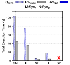
(a) P1.1

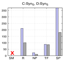
(b) P1.3

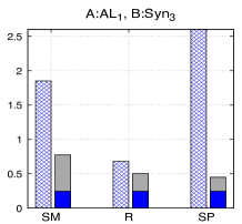
(c) P1.4

(d) P1.15

Figure 5. P1.1, P1.3, P1.4, and P1.15 evaluation before and after rewrite

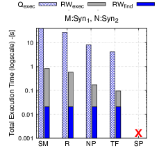
(a) P1.13

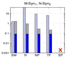
(b) P1.25

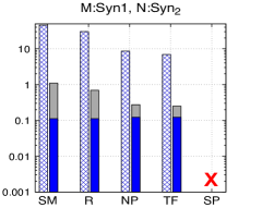
(c) P1.14

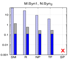
(d) P2.12

Figure 6. P1.13, P1.25, P1.14 and P2.12 evaluation before and after rewrite

For P1.1 (see Figure 5(a)), both matrices are dense. The speed-up ($1.3\times$ to $4\times$) comes from rewriting $(MN)^{T}$ (intermediate result size to $(50K)^{2}$) into $N^{T}M^{T}$, much cheaper since both $N^{T}$ and $M^{T}$ are of size $50K\times 100$. We exclude MLlib from this experiment since it failed to allocate memory for the intermediate matrix (Spark/MLLib limits the maximum size of a dense matrix). As a variation (not plotted in the Figure), we ran the same pipeline with the ultra-sparse $AS$ matrix (0.0075% non-zeros) used as $M$. The $Q_{exec}$ and $RW_{exec}$ time are very comparable using SystemML, because we avoid large dense intermediates. In R, this scenario lead to a runtime exception and to avoid it, we cast $M$ during load time to a dense matrix type. Thus, the speed-up achieved is the same as if $M$ and $N$ were both dense. If, instead, $NS$ (1.3911% non-zeros) plays the role of $M$, our rewrite achieves $\approx$ $1.8\times$ speed-up for SystemML.

For P1.3 (Figure 5(b)), the speed-up comes from rewriting $C^{-1}D^{-1}$ to $(DC)^{-1}$. Interestingly, for TensorFlow, the $Q_{exec}$ and $RW_{exec}$ time are very comparable. SystemML timed-out ($>$1000 secs) for both original pipeline and its rewriting.

For pipeline P1.4 (Figure 5(c)), we rewrite $(A+B)v_{1}$ to $Av_{1}+Bv_{1}$. Adding a sparse matrix $A$ to a dense matrix $B$ results into materializing a dense intermediate of size $1M\times 100$. Instead, $Av_{1}+Bv_{1}$ has fewer non-zeros in the intermediate results, and $Av_{1}$ can be computed efficiently since $A$ is sparse. The MNC sparsity estimator has a noticeable overhead here. We run the same pipeline, where the dense $Syn_{4}$ matrix plays both $A$ and $B$ (not shown in the Figure). This leads to speed-up of up to $9\times$ for MLlib, which does not natively support matrix addition, thus we convert its matrices to Breeze types in order to perform it (as in (thomas2018comparative, )).

P1.15 (Figure 5(d)) is a matrix chain multiplication. The naïve left-to-right evaluation plan $(MN)M$ computes an intermediate matrix of size $O(n^{2})$, where $n$ is $50K$. Instead, the rewriting $M(NM)$ only needs an $O(m^{2})$ intermediate matrix, where $m$ is $100$, and is much faster. To avoid MLLib memory failure on P1.15, we use the distributed matrix of type BlockMatrix for both matrices. While $M$ thus converted has the same sparsity, Spark views it as being of a dense type ( multiplication on BlockMatrix is considered to produce dense matrices) (sparkmlib, ). SystemML does optimize the multiplication order if the user does not enforce it. Further (not shown in the Figure), we ran P.15 with $AS$ in the role of $M$. This is $4\times$ faster in SystemML since with an ultra sparse $M$, multiplication is more efficient. This is not the case for MLlib which views it as dense. For R, we again had to densify $M$ during loading to prevent crashes.

Figures 6(a) and  6(b) study P1.13 and P1.25, two real-world pipelines involved in ML algorithms, using the MNC cost model; note the log-scale $y$ axis. Rewriting P1.13 to $\texttt{sum}(t(\texttt{colSums}((M))*\texttt{rowSums}(N))$ yields a speed-up of $50\times$; while SystemML has this rewrite as a dynamic rewrite rule, it did not apply it. In addition, our rewrite allows other systems to benefit from it. Not shown in the Figure, we re-ran this with $M$ ultra sparse (using $AS$) and SystemML: the rewrite did not bring benefits, since $MN$ is already efficient. In this experiment and subsequently, whenever MLlib is absent, this is due to its lack of support for LA operations (here, sum of all cells in a matrix) on BlockMatrix. For P1.25, the important optimization is selecting the multiplication order in $MNN^{T}$ (Figure 6(b)). SystemML is efficient here, due to its dedicated operator tsmm for transpose-self matrix multiplication and mmchain for matrix multiply chains.

Figures 6(c) and  6(d) shows up to $42\times$ rewriting speed-up achieved by turning P1.14 and P2.12 into $\texttt{sum}(t(\texttt{colSums}((M))*\texttt{rowSums}(N))$. This exploits several properties: $(i)$ $(MN)^{T}=N^{T}M^{T}$, $(ii)$ $\texttt{sum}(M^{T})=\texttt{sum}(M)$, $(iii)$ $\texttt{sum}(row/\texttt{colSums}((M))=\texttt{sum}(M)$, and $(iv)$ $\texttt{sum}(MN)=\texttt{sum}(t(\texttt{colSums}((M))*\texttt{rowSums}(N))$. SystemML captures $(ii)$, $(iii)$, and $(iv)$ as static rewrite rules, however, it is unable to exploit these performance-saving opportunities since it is unaware of $(i)$. Other systems lack support for more or all of these properties.

Figure 8 shows the distribution of the significant rewriting speed-up on $\mathcal{P}^{\neg Opt}$ running on R, and using the MNC-based cost model. For clarity, we split the distribution into two figures: on the left, 25 $\mathcal{P}^{\neg Opt}$ pipelines with speed-up lower than $10\times$; on the right, the remaining 13 with greater speed-up. Among the former, 87% achieved at least $1.5\times$ speed-up. The latter are sped up by $10\times$ to $60\times$. P1.5 is an extreme case here (not plotted): it is sped up by about $1000\times$, simply by rewriting $((D)^{-1})^{-1}$ into $D$.

(a) P2.14

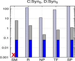
(b) P2.21

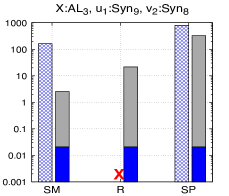
(c) P2.25

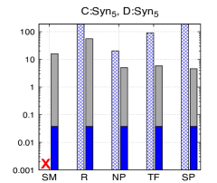
(d) P2.27

Figure 7. P2.14, P2.21, P2.25 and P2.27 evaluation before and after rewriting using the views $V_{exp}$

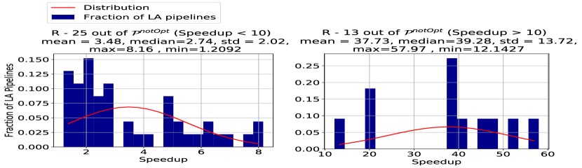
Figure 8. R speed-up on $\mathcal{P}^{\neg Opt}$

9.1.2. Effectiveness of view-based LA rewriting

We have defined a set $V_{exp}$ of 12 views that pre-compute the result of some expensive operations (multiplication, inverse, determinant, etc.) which can be used to answer our $\mathcal{P}^{Views}$ pipelines, and materialized them on disk as CSV files. The experiments outlined below used the naïve cost model; all graphs have a log-scale $y$ axis.

Discussion. For P2.14 (Figure 7(a)), using the view $V_{4}=NM$ by and the multiplication associativity leads to up to $2.8\times$ speed-up.

Figure 7(b) shows the gain due to the view $V_{1}=D^{-1}$, for the ordinary-least regression (OLS) pipeline P2.21. It has 8 rewritings, 4 of which use $V_{1}$; they are found thanks to the properties $(CD)^{-1}=D^{-1}C^{-1}$, $(CD)E=C(DE)$ and $(D^{T})^{-1}=(D^{-1})^{T}$ among others. The cheapest rewriting is $V(V^{T}(D^{T}v_{1}))$, since it introduces small intermediates due to the optimal matrix chain multiplication order. This rewrite leads to $70\times$, $55\times$ and $150\times$ speed-ups on R, NumPy and MLlib, respectively. On SystemML, the original pipeline timed out ($>1000$ seconds).

Pipeline P2.25 (Figure 7(c)) benefits from a view $V_{5}$, which pre-computes a dense intermediate vector multiplication result; then, rewriting based on the property $(A+B)v=Av+Bv$ leads to a $65\times$ speed-up in SystemML. For MLlib, as discussed before, to avoid memory failure, we used BlockMatrix types. for all matrices and vectors, thus they were treated as dense. In R, the original pipeline triggers a memory allocation failure for the intermediate result, which the rewriting avoids. Figure 7(d) shows that for P2.27 exploiting the views $V_{2}=(D+C)^{-1}$ and $V_{3}=DC$ leads to speed-ups of $4\times$ to $41\times$ on different systems. Properties enabling rewriting here are $C+D=D+C$, $(D^{T})^{-1}=(D^{-1})^{T}$ and $(CD)E=C(DE)$.

9.1.3. Rewriting Performance and Overhead

We now study the running time $RW_{find}$ of our rewriting algorithm, and the rewrite overhead defined as $RW_{find}$/($Q_{exec}$+ $RW_{find}$), where $Q_{exec}$ is the time to run the pipeline “as stated”. We ran each experiment $100$ times and report the average of the last $99$ times. The global trends are as follows. ($i$) For a fixed pipeline and set of data matrices, the overhead is slightly higher using the MNC cost model, since histograms are built during optimization. ($ii$) For a fixed pipeline and cost model, sparse matrices lead to a higher overhead simply because $Q_{exec}$ tends to be smaller. ($iii$) Some (system, pipeline) pairs lead to a low $Q_{exec}$ when the system applies internally the same optimization that HADAD finds “outside” of the system.

Concretely, for the $\mathcal{P}^{\neg Opt}$ pipelines, on the dense and sparse matrices listed in Table 6, using the naïve cost model, 64% of the $RW_{find}$ times are under 25ms (50% are under 20ms), and the longest is about 200m. Using the MNC estimator, 55% took less than 20ms, and the longest (outlier) took about 300ms. Among the 38 $\mathcal{P}^{\neg Opt}$ pipelines, SystemML finds efficient rewritings for a set of 9, denoted $\mathcal{P}^{\neg Opt}_{SM}$, while TensorFlow optimizes a different set of 11, denoted $\mathcal{P}^{\neg Opt}_{TF}$. On these subsets, where HADAD’s optimization is redundant, using dense matrices, the overhead is very low: with the MNC model, 0.48% to 1.12% on $\mathcal{P}^{\neg Opt}_{SM}$ (0.64% on average), and 0.0051% to 3.51% on $\mathcal{P}^{\neg Opt}_{TF}$ (1.38% on average). Using the naïve estimator slightly reduces this overhead, but across $\mathcal{P}^{\neg Opt}$, this model misses 4 efficient rewritings. On sparse matrices, the overhead is at most 4.86% with the naïve estimator and up to 5.11% with the MNC one.

Among the already-optimal pipelines $\mathcal{P}^{Opt}$, 70% involve expensive operations such as inverse, determinant, matrix exponential, leading to rather long $Q_{exec}$ times. Thus, the rewriting overhead is less than 1% of the total time, on all systems, using sparse or dense matrices, and the naïve or the MNC-based cost models. For the other $\mathcal{P}^{Opt}$ pipelines with short $Q_{exec}$, mostly matrix multiplications chains already in the optimal order, on dense matrices, the overhead reaches 0.143% (SparkMlLib) to 9.8% (TensorFlow) using the naïve cost model, while the MNC cost model leads to an overhead of 0.45% (SparkMlib) up to 10.26% (TensorFlow). On sparse matrices, using the naïve and MNC cost models, the overhead reaches up to 0.18% (SparkMLlib) to 1.94% (SystemML), and 0.5% (SparkMLlib) to 2.61% (SystemML), respectively.

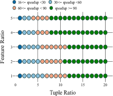
(a) P1.12

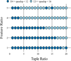
(b) P2.10

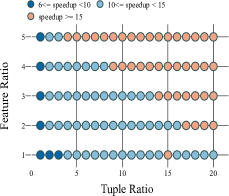
(c) P2.11

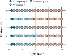
(d) P2.15

Figure 9. Speed-ups of Morpheus (with HADAD rewrites) over Morpheus (without HADAD rewrites) for pipelines P1.12, P2.10, P2.11 and P2.15 on synthetic data for a PK-FK join.

9.2. Hybrid (LA and RA) Experiments

We now study the benefits of rewriting on hybrid scenarios combining RA and LA operations. In §9.2.1, we show the performance benefits of HADAD to a cross RA-LA platform, MorpheusR (morpheus, ). We evaluate our hybrid micro-benchmark on SparkSQL+SystemML in §9.2.2. (§9.2.3) discusses our optimization overhead.

9.2.1. MorpheusR Experiments

We use the same experimental setup introduced in  (chen2017towards, ) for generating synthetic datasets for the PK-FK join of tables R and S. The quantities varied are the tuple ratio ($n_{S}$/$n_{R}$) and feature ratio ($d_{R}$/$d_{S}$), where $n_{S}$ and $n_{R}$ are the number of rows and $d_{R}$ and $d_{S}$ are the number of columns (features) in R and S, respectively. We fix $n_{R}=1M$ and $d_{S}=20$. The join of R and S outputs $n_{s}\times(d_{R}+d_{S})$ matrix M, which is always dense. We evaluate on Morpheus a set of 8 pipelines and their rewritings found by HADAD using the naïve cost model.

Discussion. P1.12: colSums$($M$N)$ is the example from §2, with M the output (viewed as matrix) of joining tables R and S generated as described above. $N$ is a $ncol($M$)\times 100$ dense matrix. HADAD’s rewriting yields up to 125$\times$ speed-up (see Figure 9(a)).

Figure 9(b) shows up to 15$\times$ speed-up for P2.10: rowSums$(N$M$)$, where the size of $N$ is $100\times nrow($M$)$. This is due to HADAD’s rewriting: $N$rowSums$($M$)$, which enables Morpheus to push the rowSums operator to R and S instead of computing the large intermediate matrix multiplication.

P2.11: sum$(N+$M$)$ is run as-is by Morpheus since it does not factorize element-wise operations, e.g., addition. However, HADAD rewrites P2.11 into sum$(N)+$sum$($M$)$, which avoids the (large and dense) intermediate result of the element-wise matrix addition. The HADAD rewriting enables Morpheus to execute sum$($M$)$ by pushing sum to R and S, for up to 20$\times$ speed-up (see Figure 9(c)).

Morpheus evaluates P2.15: sum$($rowSums$($M$))$ by pushing the rowSums operator to R and S. HADAD finds the rewriting $\texttt{sum}($M$)$, which enables Morpheus to push the sum operation instead, achieving up to 4.5$\times$ speed-up (see Figure 9(d)).

Since Morpheus does not exploit the associative property of matrix multiplication, it cannot reorder multiplication chains to avoid large intermediate results, which lead to runtime exception in R (Morpheus’ backend). For example, for the chain $N^{T}N$M (in P1.26), when the size of M is 1M$\times$20 and the size of $N$ is 20$\times$1M, the size of the $N^{T}N$ intermediate result is 1M$\times$1M, which R cannot handle ((timed out ¿1000 seconds)). HADAD exploits associativity and selects the rewriting $N^{T}(N$M$)$ of intermediate result size (100$\times$20).

For pipelines P1.14 and P2.12, that involve transpose operator, Morpheus applies its special rewrite rules that replace an operation on M^T with an operation on M before pushing the operation to the base tables. HADAD rewrites both pipelines to sum$(N$M$)$, enabling again Morpheus to apply its factorized rewrite rule on $N$M and achieving speed-up ranging from 1.3 up to 1.5$\times$.

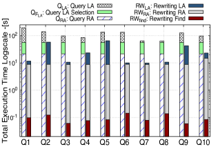
(a) N matrix: 2M rows

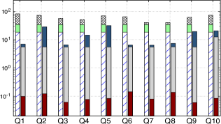
(b) N matrix: 1M rows

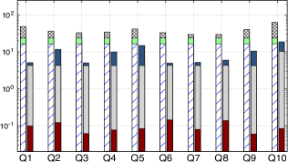
(c) N matrix : 0.5 rows

Figure 10. Micro-Hybrid Benchmark Twitter Dataset

9.2.2. Micro-hybrid Benchmark Experiments

In this experiment, we create a micro-hybrid benchmark on Twitter(twitter, ) and MIMIC (MIMIC, ) datasets to empirically study HADAD’s rewriting benefits in a hybrid setting. The benchmark comprises ten different queries combining relational and linear algebra expressions.

Twitter Dataset Preparation. We obtain from Twitter API  (twitter, ) 16GB of tweets (in JSON). We extract the structural parts of the dataset, which include user and tweet information, and store them in tables User (U) and Tweet (T), linked via PK-FK relationships. The dataset is detailed in §2. The tables User and Tweet as well as TweetJSON (TJ) are stored in Parquet format.

Twitter Queries and Views. Queries consist of two parts: ($i$) RA preprocessing ($Q_{RA}$) and ($ii$) LA analysis ($Q_{LA}$). In the $Q_{RA}$ part, queries construct two matrices: M and N. The matrix M (2M$\times$12;dense) is the output of joining T and U. The construction of matrix N is described in §2. We fix the $Q_{RA}$ part across all queries and vary the $Q_{LA}$ part using a set of LA pipelines detailed below.

In addition to the views defined in §2, we define three hybrid RA-LA materialized views: $V_{3}$, $V_{4}$ and $V_{5}$, which store the result of applying rowSums, colSums and matrix multiplication operations over base tables T and U (viewed as matrices).

Importantly, rewritings based on these views can only be found by exploiting together LA properties and Morpheus’ rewrites rules (we incorporated them in our framework as a set of integrity constraints). The full list of queries and views is in Appendix G.

No.	Expression
P3.1	rowSums$(X$M$)+(uv^{T}+$ N${}^{T})v$
P3.2	ucolSums$((X$M$)^{T})$+N
P3.3	$(($N$+X)v)$colSums$($M$)$
P3.4	$\texttt{sum}(C+$NrowSums$(X$M$)v)$
P3.5	$u$colSums$($M$X)$+N
P3.6	rowSums$(($M$X)^{T})+(uv^{T}+$ N$)v$
P3.7	$X$N$u+$rowSums$($M$)^{T}$
P3.8	N$\odot$trace$(C+v$colSums$($M$X)C)$
P3.9	$X\odot$sum$($colSums(C)${}^{T}+$rowSums$($M$))$+N
P3.10	N$\odot$ sum$((X+C)$M$)$

Table 7. LA pipelines used in micro-hybrid benchmark

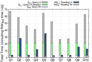
(a) N matrix: 40K rows

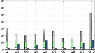
(b) N matrix: 20K rows

(c) N matrix : 10K rows

Figure 11. Micro-Hybrid Benchmark MIMIC

Discussion. After construction of M and N by the $Q_{RA}$ part in SparkSQL, both matrices are loaded to SystemML to be used in the $Q_{LA}$ part. Before evaluating an LA pipeline on M and N, all queries select N ’s rows ($Q_{F_{LA}}$) with filter-level less than $4$ (medium). For all of them, HADAD rewrites the $Q_{RA}$ part of N as described in §2.

Q1: For the $Q_{LA}$ part , the query runs P3.1 (see Table 7). HADAD applies several optimizations: ($i$) it rewrites $(uv^{T}+$ N ${}^{T})v$ to $uv^{T}v+$N${}^{T}v$, where $u$ and $v$ are synthetic vectors of size 12$\times$1 and 2M$\times$1. First, N  is ultra sparse, which makes the computation of N${}^{T}v$ extremely efficient. Second, SystemML evaluates $uv^{T}v$ efficiently in one go without intermediates, taking advantage of tsmm operator (discussed earlier) and mmchain for matrix multiply chains, where the best way to evaluate it computes $v^{T}v$ first, which results in a scalar, instead of computing $uv^{T}$, which results in a dense matrix of size 1000$\times$2M. Alone, SystemML is unable to exploit its own efficient operations for lack of awareness of the LA property $Av+Bv=(A+B)v$; ($ii$) HADAD also rewrites rowSums$(X$M$)$ into $XV_{3}$, where $V_{3}=$rowSums$($T$)$ $+K$rowSums$($U$)$, by exploiting the property rowSums$(X$M$)=X$rowSums$($M$)$ together with Morpheus’s rewrite rule: rowSums$($M$)\rightarrow$ rowSums$($T$)+K$rowSums$($U$)$ The rewriting achieves up to 16.5$\times$ speed-up.

Q2: The speed-up of 2.5$\times$ comes from rewriting the pre-processing part and turning P3.2: $u$colSums$((X$M$)^{T})$+N  to $u(XV_{4})^{T}$+N, where $u$ and $X$ are synthetic matrices of size 2M$\times$1 and 1000$\times$2M, respectively. HADAD exploits colSums$((X$M$)^{T})=$rowSums$(X$M$)^{T}$ and rowSums$(X$M$)=X$rowSums$($M$)$ together with Morpheus’s rewrite rule: rowSums$($M$)\rightarrow$ rowSums$($T$)+K$rowSums$($U$)$. Both the rewriting and the original LA pipeline introduce an unavoidable large dense intermediate of size 2M$\times$1000.

Q3: The query runs $(($N$+X)v)$colSums$($M$)$ in the $Q_{LA}$ part, where dense matrices $X$ and $v$ are of size 2M$\times$1000 and 1000$\times$1, respectively. HADAD avoids the dense intermediate (N$+X$) by distributing the multiplication by $v$ and realizing that the sparsity of N yields efficient multiplication. It also directly rewrites colSums$($M$)$ to $V_{4}$, where $V_{4}=[$colSums$($T$),$colSums$(K)$U$]$ by utilizing one of Morpheus’s rewrite rules. The rewriting, including the rewriting of the $Q_{RA}$ part of N, achieves 9.2$\times$ speed-up (Figure 10(a)-Q3).

Q4: In the $Q_{LA}$ part, Q4 runs sum$(C+$NrowSums$(X$M$)v)$ (inspired by the COX proportional hazard regression model used in SystemML’s test suite (cox, )), where synthetic dense matrices $C$, $X$ and $v$ have size 2M$\times$1000,1000$\times$2M and 1$\times$1000, respectively. HADAD ($i$) distributes the sum operation to avoid materializing the dense addition (SystemML includes this rewrite rule but fails to apply it); ($ii$) rewrites rowSums$(X$M$)$ to $XV_{3}$, where $V_{3}=$rowSums$($T$)$ $+K$rowSums$($U$)$, by exploiting rowSums$(X$M$)=X$rowSums$($M$)$ together with Morpheus’s rewrite rule rowSums$($M$)\rightarrow$ rowSums$($T$)+K$rowSums$($U$)$. The multiplication chain in the rewriting is efficient since N is sparse. The rewriting of this query (including the rewriting of the $Q_{RA}$ part of N ) achieves 3.63$\times$ speed-up (Figure 10(a)-Q4).

Q5: HADAD’s rewriting speeds-up this query by 2.3$\times$. It rewrites $u$colSums$($M$X)$ in P3.5 to $uV_{4}X$ (see Q3 for $V_{4}$’s definition). The view is exploited by HADAD  due to utilizing colSums$($M$X)$ = colSums$($M$)X$ together with the Morpheus’s rewrite rule (shown in Q3) for pushing the colSums to the base tables (matrices) U and T. The found rewriting enables SystemML to optimize the matrix-chain multiplication by computing $V_{3}X$ first, which results in 1$\times$1000 matrix instead of computing $uV_{3}$ which results in 2M$\times$12. The rewriting and the original pipeline still introduce unprevenbted dense intermediate of size 2M$\times$1000.

Q6: The LA pipeline (P3.6) in this query is a variation of P3.1. In addition to distributing the multiplication of $v$, HADAD rewrites rowSums$(($M $X)^{T})$ to $(V_{4}X)^{T}$ (see Q3 for $V_{4}$’s definition) by exploiting rowSums$(($M$X)^{T})$ = colSums$($M$X)^{T}$ and colSums$($M$X)$ = colSums$($M$)X$, all together with Morpheus’s rewrite rule as illustrated in Q3. The obtained rewriting (along with the rewriting of the pre-processing part) achieves speed-up of 13.4$\times$ .

Q8: The $Q_{LA}$ part executes N$\odot$trace$(C+v$colSums$($M$X)C)$, where the size of $v$, $X$ and $C$ are 20K$\times$1, 12$\times$20K and 20K$\times$20K, respectively. First, HADAD distributes the trace operation (which SystemML does not apply) to avoid the dense intermediate addition. Second, HADAD enables the exploitation of view $V_{4}$ (see Q2) by utilizing colSums$($M$X)$ = colSums$($M$)X$. The resulting multiplication chain is optimized by the order $v((V_{4}X)C)$. The final element-wise multiplication with N is efficient since N is ultra-sparse. The combined $Q_{RA}$ and $Q_{LA}$ rewriting speeds up Q8 by 5.94$\times$ (Figure 10(a)-Q8).

Q9: In addition to the rewriting of the $Q_{RA}$ part, the speed-up of 3$\times$ also attributes to turning sum$($colSums$(C)^{T}+$rowSums$($M$))$ in P3.9 to sum$(V_{5})$, where $V_{5}=[C$T$,CK$U$]$. The view $V_{5}$ is utilized by exploiting the property sum$(C$M$)=$sum$($colSums$(C)^{T}\odot$ rowSums$($M$))$ together with Morpheus’s rewrite rule: $C$M$\rightarrow$ $[C$T$,CK$U$]$. The result of an element-wise multiplication with the dense matrix $X$ in the rewriting and the original pipelines is a dene intermediate (see Figure  10(a)-Q9).

Q10: HADAD’s rewrite the $Q_{LA}$: N$\odot$sum$((X+C)$M$)$, where $X$ and $C$ are dense matrices of size 1000$\times$1M, to N$\odot$sum$(X$M$)+$sum$(V_{5})$. The $V_{5}=[C$T$,CK$U$]$ is utilized by exploiting $(X+C)$M= $X$M$+C$M together with Morpheus’s rewrite rule: $C$M$\rightarrow$ $[C$T$,CK$U$]$. This optimization goes beyond SystemML’s optimization since it does not consider distributing the multiplication of M, which then enables exploiting the view and distributing the sum operation to avoid a dense intermediate. The obtained rewriting (with the rewriting of the $Q_{RA}$ part of N) achieves 3.91$\times$ (Figure 10(a)-Q8).

Twitter Varying Filter Selectivity. We repeat the benchmark for two different text-search selection conditions: “Trump” and “US election”, obtaining 1M and 0.5M rows for N, respectively (we adjust the size of the synthetic matrices for dimensional compatibility). As shown in Figures 10(b) and  10(c), the benefit of the combined $Q_{RA}$ and $Q_{LA}$ stage rewriting increases with data size, remaining significant across the spectrum.

MIMIC Dataset Preparation. MIMIC dataset (MIMIC, ) comprises health data for patients. The total size of the dataset is 46.6 GB, and it consists of : (i) all charted data for all patients and their hospital admission information, ICU stays, laboratory measurements, caregivers’ notes, and prescriptions; (ii) the role of caregivers (e.g., MD stands for “medical doctor”), (iii) lab measurements (e.g., ABG stands for “arterial blood gas”) and (iv) diagnosis related groups (DRG) codes descriptions. We use subset of the dataset, which includes Patients (P), Admission (A), Service (S), and Callout (C) tables. We convert tables’ categorical features (columns) to numeric using one-hot encoding.

MIMIC Queries and Views. Similar to the Twitter’s dataset benchmark, queries consist of two parts: ($i$) preprocessing ($Q_{RA}$) and ($ii$) analysis ($Q_{LA}$). In the $Q_{RA}$ part, the queries construct two main matrices: M and N. The matrix M (40K$\times$82;dense) is the join’s output table (matrix) of P and A. The matrix N (40K$\times$30K;ultra-sparse) is patient-service outcome (e.g., cancelled (1), serving (2), etc) matrix, constructed from joining C and S for all patients who are in “CCU” care unit. We fix the $Q_{RA}$ part across all queries and vary the $Q_{LA}$ part using a set of LA pipelines in Table  7, a well as N  and M matrices. For views, we define three cross RA-LA materialized views: $V_{1}$, $V_{2}$ and $V_{3}$, which store the result of applying rowSums, colSums and matrix multiplication operations over P and A base tables (matrices), respectively. These views can only be found by exploiting together LA properties and Morpheus rewrites’ rules in the same fashion as we detailed in Twitter’s benchmark experiment.

Discussion. The results exhibit similar trends to the Twitter’s benchmark. The first run of the benchmark is shown in Figure 11(a); both matrices M  and N are loaded in SystemML to be used for the analysis part (varied using the set of pipelines in Table 7). Before evaluating an LA pipeline, all queries filter N ’s rows with outcome is equal to 2. HADAD applies the same set of optimizations as described in Twitter’s benchmark. For the second and third runs of the queries (see Figures  11(b) and  11(c)), we construct the N matrix for patients who are in “TSICU” and “MICU” care units, where N’s rows are 20K and 10K, respectively.

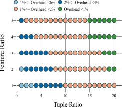
(a) P1.10

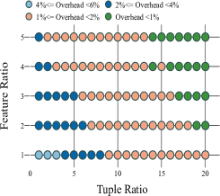
(b) P1.16

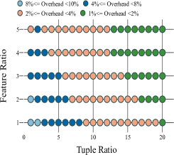
(c) P1.18

Figure 12. HADAD $RW_{find}$ overhead as a percentage (%) of the total time ($Q_{exec}+RW_{fond}$) for pipelines P1.1, P1.10, P1.13, P1.16 and P1.18 running on Morpheus

9.2.3. Rewriting Time Overhead

For MorpheusR, using the same experiment setup illustrated in §9.2.1, the rewriting time’s overhead is very negligible compared to the pipelines’ execution time for pipelines that are already optimized or MorpheusR finds the same rewriting found by HADAD. For pipelines that contain matrix multiplication expressions, the rewriting time is generally less than 0.1% of the total time. However, for the other pipelines such as P1.10, P1.16, and P1.18, which contain only aggregate operations, the rewriting time is up to 9% of the total time (when the data size is very small (0.32GB) and the computation is extremely efficient) and less than 1% (when the data size is large (19.2GB) and the computation is expensive) as shown in Figure  12.

9.3. Experiments Takeaway

Our experiments with both real-life and synthetic datasets show performance gains across the board, for small rewriting overhead, in both pure LA and hybrid RA-LA settings. This is due to the fact that HADAD’s rewriting power strictly subsumes that of optimizers of reference platforms like R, Numpy, TensorFlow, Spark (MLlib), SystemML and Morpheus. Moreover, HADAD enables optimization where it wasn’t previously feasible, such as across a cascade of unintegrated tools, e.g. SparkSQL for preprocessing followed by SystemML for analytics.

10. Related Work and Conclusion

LA Systems/Libraries. SystemML (boehm2016systemml, ) offers high-level R-like LA language and applies some logical LA pattern-based rewrites and physical execution optimizations, based on cost estimates for the latter. SparkMLlib (meng2016mllib, ) provides LA operations and built-in function implementations of popular ML algorithms on Spark RDDs. R (R, ) and NumPy (NumPy, ) are two of the most popular computing environments for statistical data analysis, widely used in academia and industry. They provide a high-level abstraction that can simplify the programming of numerical and statistical computations, by treating matrices as first-class citizens and by providing a rich set of built-in LA operations. However, LA properties in most of these systems remain unexploited, which makes them miss opportunities to use their own highly efficient operators (recall hybrid-scenario in §2). Our experiments (§9.1) show that LA pipelines evaluation in these systems can be sped up, by more than $10\times$, by our rewriting using ($i$) LA properties and ($ii$) materialized views.

Bridging the Gap: RA and LA. There has been a recent increase in research for unifying the execution of RA and LA expressions (luo2018scalable, ; montdb, ; kernert2013bringing, ; chen2017towards, ). A key limitation of these approaches is that the semantics of LA operations remains hidden behind built-in functions or UDFs, preventing performance-enhancing rewrites as shown in §9.2.1.

SPORES (spores, ), SPOOF (boehm2018optimizing, ), LARA (kunft2019intermediate, ) and RAVEN  (aranasosIPSPPX20, ) are closer to our work. SPORES and SPOOF optimize LA expressions, by converting them into RA, optimizing the latter, and then converting the result back to an (optimized) LA expression. They are restricted to a small set of selected LA operations (the ones that can be expressed in RA), while we support significantly more (§6.1), and model properties allowing to optimize with them. LARA relies on a declarative domain-specific language for collections and matrices, which can enable optimization (i.e., selection pushdown) across the two algebraic abstractions. It heavily focuses on low-level optimization such as exploiting the choice of data layouts for physical LA operators’ optimization. RAVEN takes a step forward by providing intermediate representation to enhance in-database model inferencing performance. It transforms classical ML models into equivalent neural networks to leverage highly optimized ML engines on CPU/GPU. (BarceloH0S20, ; BrijderGBW19, ) study the expressive power of corss RA-LA (BarceloH0S20, ) / LA (BrijderGBW19, ) query languages. In contrast to HADAD, as all aforementioned solutions do not reason with constraints, they provide no capabilities for holistic semantic query optimizations including RA/LA views-based and LA pure rewritings; such optimizations can bring large performance saving as shown in §9.

We see HADAD as complementary to all of these platforms, on top of which it can be naturally and portably applied.

Conclusion. HADAD is an extensible lightweight framework for optimizing hybrid analytics queries, based on the powerful intermediate abstraction of a a relational model with integrity constraints. HADAD extends the capability of  (estocada-sigmod, ) with a reduction from LA (or LA view)-based rewriting to relational rewriting under constraints. It enables a full exploration of rewrites using a large set of LA operations, with no modification to the execution platform. Our experiments show significant performance gains on various LA and hybrid workloads across popular LA and cross RA-LA platforms.

Appendix A $L_{ops}$ Operations Properties ($LA_{prop}$) Captured as Integrity Constraints

Table 8. $L_{ops}$ Operations Properties ($LA_{prop}$) Captured as Integrity Constraints

LA Property	Relational Encoding as Integrity Constraints
Addition of Matrices
$M+N=N+M$	$\forall M,N,R$ addM$(M,N,R)\rightarrow$ addM$(N,M,R)$
$(M+N)+D=M+(N+D)$	$\forall M,N,D,R_{1},R_{2}$   addM$(M,N,R_{1})\wedge$ addM$(R_{1},D,R_{2})\rightarrow$
	$\exists R_{3}$ addM$(N,D,R_{3})\wedge$ addM$(M,R_{3},R_{2})$
$c(M+N)=cM+cN$	$\forall c,M,N,R_{1},R_{2}$   addM$(M,N,R_{1})\wedge$ multiMS$(c,R_{1},R_{2})\rightarrow$
	$\exists R_{3},R_{4}\texttt{multi${}_{MS}$}(c,M,R_{3})\wedge\texttt{multi${}_{MS}$}(c,N,R_{4})\wedge\texttt{add${}_{M}$}(R_{3},R_{4},R_{2})$
$(c+d)M=cM+dM$	$\forall c,d,s,M,R_{1}add_{S}(c,d,s)\wedge\texttt{multi${}_{MS}$}(s,M,R_{1})\rightarrow$
	$\exists R_{2},R_{3}\texttt{multi${}_{MS}$}(c,M,R_{2})\wedge\texttt{multi${}_{MS}$}(d,M,R_{3})\wedge\texttt{add${}_{M}$}(R_{2},R_{3},R_{1})$
$M+0=M$	$\rightarrow\exists Zero(O)$
	$\forall M,n,O$   $name(M,n)\wedge Zero(O)\rightarrow\texttt{add${}_{M}$}(M,O,M)$
	$\forall O$   $Zero(O)\rightarrow\texttt{add${}_{M}$}(O,O,O)$
Product of Matrices
$(MN)D=M(ND)$	$\forall M,N,D,R_{1},R_{2}$  $\texttt{multi${}_{M}$}(M,N,R_{1})\wedge\texttt{multi${}_{M}$}(R_{1},D,R_{2})\rightarrow$
	$\exists R_{3}\texttt{multi${}_{M}$}(N,D,R_{3})\wedge\texttt{multi${}_{M}$}(M,R_{3},R_{2})$
$M(N+D)=MN+MD$	$\forall M,N,D,R_{1},R_{2}$   $\texttt{add${}_{M}$}(N,D,R_{1})\wedge\texttt{multi${}_{M}$}(M,R_{1},R_{2})\rightarrow$
	$\exists R_{3},R_{4}$ $\texttt{multi${}_{M}$}(M,N,R_{3})\wedge\texttt{multi${}_{M}$}(M,D,R_{4})\wedge\texttt{add${}_{M}$}(R_{3},R_{4},R_{2})$
$(M+N)D=MD+MD$	$\forall M,N,D,R_{1},R_{2}\texttt{add${}_{M}$}(M,N,R_{1})\wedge\texttt{multi${}_{M}$}(R_{1},D,R_{2})\rightarrow$
	$\exists R_{3},R_{4}\texttt{multi${}_{M}$}(M,D,R_{3})\wedge\texttt{multi${}_{M}$}(N,D,R_{4})\wedge\texttt{add${}_{M}$}(R_{3},R_{4},R_{2})$
$d(MN)=(dM)N$	$\forall d,M,N,R_{1},R_{2}$   $\texttt{multi${}_{M}$}(M,N,R_{1})\wedge\texttt{multi${}_{MS}$}(d,R_{1},R_{2})\rightarrow$
	$\exists R_{3}\texttt{multi${}_{MS}$}(d,M,R_{3})\wedge\texttt{multi${}_{M}$}(R_{3},N,R_{2})$
$c(dM)=(cd)M$	$\forall c,dM,R_{1},R_{2}\texttt{multi${}_{MS}$}(d,M,R_{1})\wedge\texttt{multi${}_{MS}$}(c,R_{1},R_{2})\rightarrow$
	$\exists s$ $multi_{S}(c,d,s)\wedge\texttt{multi${}_{MS}$}(s,M,R_{2})$
$I_{k}M=M=MI_{z}$	$\forall M,n,k,z$ $name(M,n),size(M,k,z)\rightarrow\exists I$ $Identity(I),size(I,k,k)$
	$\forall M,n,k,z$ $name(M,n),size(M,k,z)\rightarrow\exists I_{1}$ $Identity(I_{1}),size(I,z,z)$
	$\forall M,I_{1},n,k,z$ $name(M,n),size(M,k,z),Identity(I),size(I_{1},k,k)\rightarrow\texttt{multi${}_{M}$}(I,M,M)$
	$\forall M,I_{1},n,k,z$ $name(M,n),size(M,k,z),Identity(I),size(I_{1},z,z)\rightarrow\texttt{multi${}_{M}$}(M,I,M)$
Transposition of Matrices
$(MN)^{T}=N^{T}M^{T}$	$\forall M,N,R_{1},R_{2}\texttt{multi${}_{M}$}(M,N,R_{1})\wedge\texttt{tr}(R_{1},R_{2})\rightarrow$
	$\exists R_{3},R_{4}\texttt{tr}(M,R_{3})\wedge\texttt{tr}(N,R_{4})\wedge\texttt{multi${}_{M}$}(R_{4},R_{3},R_{2})$
$(M+N)^{T}=M^{T}+N^{T}$	$\forall M,N,R_{1},R_{2}\leavevmode\nobreak\ \texttt{add${}_{M}$}(M,N,R_{1})\wedge\texttt{tr}(R_{1},R_{2})\rightarrow$
	$\exists R_{3},R_{4}\texttt{tr}(M,R_{3})\wedge\texttt{tr}(N,R_{4})\wedge\texttt{add${}_{M}$}(R_{3},R_{4},R_{2})$
$(cM)^{T}=c(M)^{T}$	$\forall c,M,R_{1},R_{2}\leavevmode\nobreak\ \texttt{multi${}_{MS}$}(c,M,R_{1})\wedge\texttt{tr}(R_{1},R_{2})\rightarrow$
	$\exists R_{3}\texttt{tr}(M,R_{3})\wedge\texttt{multi${}_{MS}$}(c,R_{3},R_{2})$
$((M)^{T})^{T}=M$	$\forall n,M\leavevmode\nobreak\ name(M,n)\rightarrow\exists R_{1}\texttt{tr}(M,R_{1})\wedge\texttt{tr}(R_{1},M)$
$(I)^{T}=I$, where $I$ is identity matrix	$\forall I\leavevmode\nobreak\ \leavevmode\nobreak\ Identity(I)\rightarrow\texttt{tr}(I,I)$
$(O)^{T}=O$, where $O$ is zero matrix	$\forall O\leavevmode\nobreak\ \leavevmode\nobreak\ Zero(O)\rightarrow\texttt{tr}(O,O)$
Inverses of Matrices
$((M)^{-1})^{-1}=M$	$\forall n,M\leavevmode\nobreak\ name(M,n)\rightarrow\exists R_{1}\texttt{inv${}_{M}$}(M,R_{1})\wedge\texttt{inv${}_{M}$}(R_{1},M)$
$(MN)^{-1}=N^{-1}M^{-1}$	$\forall M,N,R_{1},R_{2}\leavevmode\nobreak\ \leavevmode\nobreak\ \texttt{multi${}_{M}$}(M,N,R_{1})\wedge\texttt{inv${}_{M}$}(R_{1},R_{2})\rightarrow$
	$\exists R_{3},R_{4}\texttt{inv${}_{M}$}(M,R_{3})\wedge\texttt{inv${}_{M}$}(N,R_{4})\wedge\texttt{multi${}_{M}$}(R_{4},R_{3},R_{2})$
$((M)^{T})^{-1}=((M)^{-1})^{T}$	$\forall M,R_{1},R_{2}\texttt{tr}(M,R_{1})\wedge\texttt{inv${}_{M}$}(R_{1},R_{2})\rightarrow$
	$\exists R_{3}\texttt{inv${}_{M}$}(M,R_{3})\wedge\texttt{tr}(R_{3},R_{2})$
$((kM))^{-1}=k^{-1}M^{-1}$	$\forall k,M,R_{1},R_{2}\leavevmode\nobreak\ \leavevmode\nobreak\ \texttt{multi${}_{MS}$}(k,M,R_{1})\wedge\texttt{inv${}_{M}$}(R_{1},R_{2})\rightarrow$
	$\exists R_{3},s$ $inv_{S}(k,s)\wedge\texttt{inv${}_{M}$}(M,R_{3})\wedge\texttt{multi${}_{MS}$}(s,R_{3},R_{2})$
$M^{-1}M=I=MM^{-1}$	$\forall M,R_{1},R_{2}$ $\texttt{inv${}_{M}$}(M,R_{1})\wedge\texttt{multi${}_{M}$}(R_{1},M,R_{2})\rightarrow Identity(R_{2})$
	$\forall M,R_{1},R_{2}$ $\texttt{inv${}_{M}$}(M,R_{1})\wedge\texttt{multi${}_{M}$}(M,R_{1},R_{2})\rightarrow Identity(R_{2})$

Table 9. $L_{ops}$ Operations Properties ($LA_{prop}$) Captured as Integrity Constraints

LA Property	Relational Encoding as Integrity Constraints
Determinant of Matrices
$\texttt{det}(MN)=\texttt{det}(M)*\texttt{det}(N)$	$\forall M,N,R_{1},d$ $\texttt{multi${}_{M}$}(M,N,R_{1})\wedge\texttt{det}(R_{1},d)\rightarrow$
	$\exists d_{1},d_{2}\texttt{det}(M,d_{1})\wedge\texttt{det}(N,d_{2})\wedge multi_{S}(d_{1},d_{2},d)$
$\texttt{det}((M)^{T})=\texttt{det}(M)$	$\forall M,R_{1},d$ $\texttt{tr}(M,R_{1})\wedge\texttt{det}(R_{1},d)\rightarrow\texttt{det}(M,d)$
$\texttt{det}((M)^{-1})=(\texttt{det}(M))^{-1}$	$\forall M,R_{1},d$ $\texttt{inv${}_{M}$}(M,R_{1})\wedge\texttt{det}(R_{1},d)\rightarrow\exists d_{1}\texttt{det}(M,d_{1})\wedge inv_{S}(d_{1},d)$
$\texttt{det}((cM))=c^{k}\texttt{det}(M)$	$\forall M,c,k,d$ $size(M,k,k)\wedge\texttt{multi${}_{MS}$}(c,M,d)\rightarrow$ $\exists s_{1},s_{2}$
	$pow(c,k,s_{1})\wedge\texttt{det}(M,s_{2})\wedge multi_{S}(s_{1},s_{2},d)$
$\texttt{det}((I))=1$	$\forall I_{1},dIdentity(I_{1})\wedge\texttt{det}(I_{1},d)\rightarrow d=1$
Adjoint of Matrices
$\texttt{adj}(M)=R^{T}$	$\forall M,R_{1}$ $\texttt{adj}(M,R_{1})\rightarrow\exists R_{2}$ $cof(M,R_{2})\wedge\texttt{tr}(R_{2},R_{1})$
$\texttt{adj}(M)^{T}=\texttt{adj}(M^{T})$	$\forall M,R_{1},R_{2}$ $\texttt{adj}(M,R_{1})\wedge\texttt{tr}(R_{1},R_{2})\rightarrow$ $\exists R_{3}$ $\texttt{tr}(M,R_{3})\wedge\texttt{adj}(R_{3},R_{2})$
$\texttt{adj}(M)^{-1}=\texttt{adj}(M^{-1})$	$\forall M,R_{1},R_{2}$ $\texttt{adj}(M,R_{1})\wedge\texttt{inv${}_{M}$}(R_{1},R_{2})\rightarrow$ $\exists R_{3}$ $\texttt{inv${}_{M}$}(M,R_{3})\wedge\texttt{adj}(R_{3},R_{2})$
$\texttt{adj}(MN)=\texttt{adj}(N)\texttt{adj}(M)$	$\forall M,R_{1},R_{2}$ $\texttt{multi${}_{M}$}(M,N,R_{1})\wedge\texttt{adj}(R_{1},R_{2})\rightarrow$ $\exists R_{3}$ $R_{4}$
	$\texttt{multi${}_{M}$}(R_{3},R_{4},R_{2})\wedge\texttt{adj}(N,R_{3})\wedge\texttt{adj}(M,R_{4})$
Trace of Matrices
$\texttt{trace}(M+N)=\texttt{trace}(M)+\texttt{trace}(N)$	$\forall M,N,R_{1},s_{1}$ $\texttt{add${}_{M}$}(M,N,R_{1})\wedge$
	$\texttt{trace}(R_{1},s_{1})\rightarrow$ $\exists s_{2},s_{3}$ $\texttt{trace}(M,s_{2})\wedge\texttt{trace}(N,s_{3})\wedge add_{s}(s_{2},s_{3},s_{1})$
$\texttt{trace}(MN)=\texttt{trace}(NM)$	$\forall M,N,R_{1},s_{1}$ $\texttt{multi${}_{M}$}(M,N,R_{1})\wedge$
	$\texttt{trace}(R_{1},s_{1})\rightarrow$ $\exists R_{2}$ $\texttt{multi${}_{M}$}(N,M,R_{2})\wedge\texttt{trace}(R_{2},s_{1})$
$\texttt{trace}(M^{T})=\texttt{trace}(M)$	$\forall M,R_{1},s_{1}$   $\texttt{tr}(M,R_{1})\wedge\texttt{trace}(R_{1},s_{1})$ $\rightarrow\texttt{trace}(M,s_{1})$
$\texttt{trace}(cM)=c\texttt{trace}(M)$	$\forall M,R_{1},c,s_{1}$   $\texttt{multi${}_{MS}$}(c,M,R_{1})\wedge\texttt{trace}(R_{1},s_{1})$ $\rightarrow\exists s_{2}\texttt{trace}(M,s_{2})\wedge multi_{s}(c,s_{2},s_{1})$
$\texttt{trace}(I_{k})=k$	$\forall I,k,s_{1}$   $Identity(I)\wedge size(I,k,k)\wedge\texttt{trace}(I,s_{1})$ $\rightarrow s_{1}=k$
Direct Sum
$(M\oplus N)+(C\oplus D)=(M+C)\oplus(N+D)$	$\forall M,N,R_{1},C,D,R_{2},R_{3}$ $\texttt{sum${}_{D}$}(M,N,R_{1})$
	$\wedge\texttt{sum${}_{D}$}(C,D,R_{2})\wedge\texttt{add${}_{M}$}(R_{1},R_{2},R_{3})\rightarrow\exists R_{4},R_{5}\texttt{add${}_{M}$}(M,C,R_{4})\wedge\texttt{add${}_{M}$}(N,D,R_{5})$
	$\wedge\texttt{sum${}_{D}$}(R_{5},R_{3)}$
$(M\oplus N)(C\oplus D)=(MC)\oplus(ND)$	$\forall M,N,R_{1},C,D,R_{2},R_{3}$ $\texttt{sum${}_{D}$}(M,N,R_{1})$
	$\wedge\texttt{sum${}_{D}$}(C,D,R_{2})\wedge\texttt{multi${}_{M}$}(R_{1},R_{2},R_{3})\rightarrow\exists R_{4},R_{5}\texttt{multi${}_{M}$}(M,C,R_{4})\wedge\texttt{multi${}_{M}$}(N,D,R_{5})$
	$\wedge\texttt{sum${}_{D}$}(R_{5},R_{3)}$
Exponential of Matrices
$\texttt{exp}(0)=I$	$\forall O,R_{1}$  $Zero(O)\wedge\texttt{exp}(O,R_{1})\rightarrow Identity(R_{1})$
$\texttt{exp}(M^{T})=\texttt{exp}(M)^{T}$	$\forall M,R_{1},R_{2}\texttt{tr}(M,R_{1})\wedge\texttt{exp}(R_{1},R_{2})\rightarrow\exists R_{3}\texttt{exp}(M,R_{3})\wedge\texttt{exp}(R_{3},R_{2})$

Table 10. Matrix Decompositions Properties Captured as Integrity Constraints

Decomposition Property	Relational Encoding as Integrity Constraints
Cholesky Decomposition (CD)
$\texttt{CHO}(M)=L$ such that $M=LL^{T}$, where M is symmetric positive definite	$\forall M\leavevmode\nobreak\ type(M,``S")\rightarrow\exists$   $L_{1}\exists L_{2}\leavevmode\nobreak\ \texttt{CHO}(M,L_{1})\wedge type(L_{1},``L")\wedge$
	$\texttt{tr}(L_{1},L_{2})\wedge\texttt{multi${}_{M}$}(L_{1},L_{2},M)$
QR Decomposition
$QR(M)=[Q,R]$ such that $M=QR$	$\forall M\forall n\forall k\leavevmode\nobreak\ name(M,n)\wedge size(M,k,k)\rightarrow\leavevmode\nobreak\ \exists Q,R$
	$QR(M,Q,R)\wedge type(Q,``O")\wedge type(R,``U")\wedge$
	$\texttt{multi${}_{M}$}(Q,R,M)$
	$\forall Q\leavevmode\nobreak\ type(Q,``O")\rightarrow\exists I\leavevmode\nobreak\ QR(Q,Q,I)\wedge identity(I)$
	$\wedge\texttt{multi${}_{M}$}(Q,I,Q)$
	$\forall R\leavevmode\nobreak\ type(R,``U")\rightarrow\exists I\leavevmode\nobreak\ QR(R,I,R)\wedge identity(I)$
	$\wedge\texttt{multi${}_{M}$}(I,R,R)$
	$\forall I\leavevmode\nobreak\ identity(I)\rightarrow QR(I,I,I)$
LU Decomposition
$\texttt{LU}(M)=[L,U]$ such that $M=LU$	$\forall M\forall n\forall k\leavevmode\nobreak\ name(M,n)\wedge size(M,k,k)\rightarrow\leavevmode\nobreak\ \exists L,U$
	$\texttt{LU}(M,L,U)\wedge type(L,``L")\wedge type(U,``U")\wedge$
	$\texttt{multi${}_{M}$}(L,U,M)$
	$\forall L\leavevmode\nobreak\ type(L,``L")\rightarrow\exists I\leavevmode\nobreak\ \texttt{LU}(L,L,I)\wedge identity(I)$
	$\wedge\texttt{multi${}_{M}$}(L,I,L)$
	$\forall U\leavevmode\nobreak\ type(U,``U")\rightarrow\exists I\leavevmode\nobreak\ \texttt{LU}(U,I,U)\wedge identity(I)$
	$\wedge\texttt{multi${}_{M}$}(I,U,U)$
	$\forall I\leavevmode\nobreak\ identity(I)\rightarrow\texttt{LU}(I,I,I)$
Pivoted LU Decomposition
$\texttt{LUP}(M)=[L,U,P]$ such that $PM=LU$, where $M$ is a square matrix	$\forall M\forall n\forall k\leavevmode\nobreak\ name(M,n)\wedge size(M,k,z)\rightarrow\leavevmode\nobreak\ \exists L,U,P,R$
	$\texttt{LUP}(M,L,U,P)\wedge type(L,``L")\wedge type(U,``U")\wedge type(P,``P")$
	$\wedge\texttt{multi${}_{M}$}(L,U,R)\wedge\texttt{multi${}_{M}$}(P,M,R)$
	$\forall L\leavevmode\nobreak\ type(L,``L")\wedge size(L,k,z)\rightarrow\exists I\leavevmode\nobreak\ \texttt{LUP}(L,L,I,I)\wedge$
	$identity(I)$ $\wedge\texttt{multi${}_{M}$}(L,I,L)\wedge\texttt{multi${}_{M}$}(I,L,L)$
	$\forall U\leavevmode\nobreak\ type(U,``U")\rightarrow\exists I\leavevmode\nobreak\ \texttt{LUP}(U,I,U,I)\wedge$
	$identity(I)\wedge\texttt{multi${}_{M}$}(I,U,U)$
	$\forall I\leavevmode\nobreak\ identity(I)\rightarrow\texttt{LU}(I,I,I)$

Appendix B SystemML Rewrite Rules Encoded As Integrity Constraints

Table 11. SystemML Algebraic Aggregate Rewrite Rules Captured as Integrity Constraints

SystemML Algebraic Simplification Rule	Integrity Constraints $\bm{\mathcal{MMC}}_{StatAgg}$
UnnecessaryAggregates
sum(t(M))-¿ sum(M)	$\forall M,R_{1},s$ $\texttt{tr}(M,R_{1}),\texttt{sum}(R_{1},s)\rightarrow\texttt{sum}(M,s)$
sum(rev(M))-¿ sum(M)	$\forall M,R_{1},s$ $rev(M,R_{1}),\texttt{sum}(R_{1},s)\rightarrow\texttt{sum}(M,s)$
sum(rowSums(M))-¿ sum(M)	$\forall M,R_{1},s$ $\texttt{rowSums}(M,R_{1}),\texttt{sum}(R_{1},s)\rightarrow\texttt{sum}(M,s)$
sum(colSums(M))-¿ sum(M)	$\forall M,R_{1},s$ $\texttt{colSums}(M,R_{1}),\texttt{sum}(R_{1},s)\rightarrow\texttt{sum}(M,s)$
min(rowMin(M))-¿ min(M)	$\forall M,R_{1},s$ $\texttt{rowMin}(M,R_{1}),\texttt{min}(R_{1},s)\rightarrow\texttt{min}(M,s)$
min(colMin(M))-¿ min(M)	$\forall M,R_{1},s$ $\texttt{colMin}(M,R_{1}),\texttt{min}(R_{1},s)\rightarrow\texttt{min}(M,s)$
max(colmax(M))-¿ max(M)	$\forall M,R_{1},s$ $\texttt{colMax}(M,R_{1}),\texttt{max}(R_{1},s)\rightarrow\texttt{max}(M,s)$
max(rowmax(M))-¿ max(M)	$\forall M,R_{1},s$ $\texttt{rowMax}(M,R_{1}),\texttt{max}(R_{1},s)\rightarrow\texttt{max}(M,s)$
pushdownUnaryAggTransposeOp
rowSums(t(M))-¿t(colSums(M))	$\forall M,R_{1},R_{2}$ $\texttt{tr}(M,R_{1})\wedge\texttt{rowSums}(R_{1},R_{2})\rightarrow\exists R_{3}$ $\texttt{colSums}(M,R_{3})\wedge\texttt{tr}(R_{3},R_{2})$
colSums(t(M))-¿t(rowSums(M))	$\forall M,R_{1},R_{2}$ $\texttt{tr}(M,R_{1})\wedge\texttt{colSums}(R_{1},R_{2})\rightarrow\exists R_{3}$ $\texttt{rowSums}(M,R_{3})\wedge\texttt{tr}(R_{3},R_{2})$
rowMean(t(M))-¿t(colMean(M))	$\forall M,R_{1},R_{2}$ $\texttt{tr}(M,R_{1})\wedge\texttt{colMean}(R_{1},R_{2})\rightarrow\exists R_{3}$ $\texttt{rowMean}(M,R_{3})\wedge\texttt{tr}(R_{3},R_{2})$
colMean(t(M))-¿t(rowMean(M))	$\forall M,R_{1},R_{2}$ $\texttt{tr}(M,R_{1})\wedge\texttt{rowMean}(R_{1},R_{2})\rightarrow\exists R_{3}$ $\texttt{colMean}(M,R_{3}\wedge\texttt{tr}(R_{3},R_{2})$
rowVar(t(M))-¿t(colVar(M))	$\forall M,R_{1},R_{2}$ $\texttt{tr}(M,R_{1})\wedge\texttt{rowVar}(R_{1},R_{2})\rightarrow\exists R_{3}$ $\texttt{colVar}(M,R_{3})\wedge\texttt{tr}(R_{3},R_{2})$
colVar(t(X))-¿t(rowVar(X))	$\forall M,R_{1},R_{2}$ $\texttt{tr}(M,R_{1})\wedge\texttt{colVar}(R_{1},R_{2})\rightarrow\exists R_{3}$ $\texttt{rowVar}(M,R_{3})\wedge\texttt{tr}(R_{3},R_{2})$
rowMax(t(M))-¿t(colMax(M))	$\forall M,R_{1},R_{2}$ $\texttt{tr}(M,R_{1})\wedge\texttt{rowMax}(R_{1},R_{2})\rightarrow\exists R_{3}$ $\texttt{colMax}(M,R_{3})\wedge\texttt{tr}(R_{3},R_{2})$
colMax(t(M))-¿t(rowMax(M))	$\forall M,R_{1},R_{2}$ $\texttt{tr}(M,R_{1})\wedge\texttt{colMax}(R_{1},R_{2})\rightarrow\exists R_{3}$ $\texttt{rowMax}(M,R_{3})\wedge\texttt{tr}(R_{3},R_{2})$
rowMin(t(M))-¿t(colMin(M))	$\forall M,R_{1},R_{2}$ $\texttt{tr}(M,R_{1})\wedge\texttt{rowMin}(R_{1},R_{2})\rightarrow\exists R_{3}$ $\texttt{colMin}(M,R_{3})\wedge\texttt{tr}(R_{3},R_{2})$
colMin(t(M))-¿t(rowMin(M))	$\forall M,R_{1},R_{2}$ $\texttt{tr}(M,R_{1})\wedge\texttt{colMin}(R_{1},R_{2})\rightarrow\exists R_{3}$ $\texttt{rowMin}(M,R_{3})\wedge\texttt{tr}(R_{3},R_{2})$
simplifyTraceMatrixMult
trace(MN)-¿sum(M$\odot$t(N))	$\forall M,N,R_{1},r$ $\texttt{multi${}_{M}$}(M,N,R_{1})\wedge\texttt{trace}(R_{1},r)\rightarrow$
	$\exists R_{3},R_{4}\texttt{tr}(N,R_{3})\wedge\texttt{multi${}_{E}$}(M,R_{3},R_{4})\wedge\texttt{sum}(R_{4},r)$
simplifySumMatrixMult
sum(MN) -¿ sum(t(colSums(M))$\odot$rowSums(N))	$\forall M,N,R_{1},r$ $\texttt{multi${}_{M}$}(M,N,R_{1})\wedge\texttt{sum}(R_{1},r)\rightarrow$
	$\exists R_{2},R_{3},R_{4},R_{5}$ $\texttt{colSums}(M,R_{2})\wedge\texttt{tr}(R_{2},R_{3})\wedge\texttt{rowSums}(N,R_{4})\wedge$
	$\texttt{multi${}_{E}$}(R_{3},R_{4},R_{5}),\wedge\texttt{sum}(R_{5},r)$
colSums(MN) -¿ colSums(M)N	$\forall M,N,R_{1},R_{2}$ $\texttt{multi${}_{M}$}(M,N,R_{1})\wedge\texttt{colSums}(R_{1},R_{2})\rightarrow$
	$\exists R_{3}$ $\texttt{colSums}(M,R_{3})\wedge\texttt{multi${}_{M}$}(R_{3},N,R_{2})$
rowSums(MN) -¿ MrowSums(N)	$\forall M,N,R_{1},R_{2}$ $\texttt{multi${}_{M}$}(M,N,R_{1})\wedge\texttt{rowSums}(R_{1},R_{2})\rightarrow$
	$\exists R_{3}$ $\texttt{rowSums}(N,R_{3})\wedge\texttt{multi${}_{M}$}(M,R_{3},R_{2})$
colSums(M)-¿M if x is row vector	$\forall M,n,i$ $name(M,n)\wedge size(M,``1",j)\rightarrow\texttt{colSums}(M,M)$
colMean(M)-¿M if x is row vector	$\forall M,n,j$ $name(M,n)\wedge size(M,``1",j)\rightarrow\texttt{colSums}(M,M)$
colVar(M)-¿M if x is row vector	$\forall M,n,j$ $name(M,n)\wedge size(v``1",j)\rightarrow\texttt{colVar}(M,M)$
colMax(M)-¿M if x is row vector	$\forall M,n,j$ $name(M,n)\wedge size(M,``1",j)\rightarrow\texttt{colMax}(M,M)$
colMin(M)-¿M if x is row vector	$\forall M,n,j$ $name(M,n)\wedge size(M,``1",j)\rightarrow\texttt{colMin}(M,M)$
colSums(M)-¿sum(M) if x is col vector	$\forall M,i,R_{1}$ $\texttt{colSums}(M,R_{1})\wedge size(M,i,``1")\rightarrow\texttt{sum}(M,R_{1})$
colMean(M)-¿mean(M) if x is col vector	$\forall M,i,R_{1}$ $\texttt{colMean}(M,R_{1})\wedge size(M,i,``1")\rightarrow\texttt{mean}(M,R_{1})$
colMax(X)-¿max(M) if x is col vector	$\forall M,i,R_{1}$ $\texttt{colMax}(M,R_{1})\wedge size(M,i,``1")\rightarrow\texttt{max}(M,R_{1})$
colMin(M)-¿min(X) if x is col vector	$\forall M,i,R_{1}$ $\texttt{colMin}(M,R_{1})\wedge size(M,i,``1")\rightarrow\texttt{min}(M,R_{1})$
colVar(M)-¿var(M) if x is col vector	$\forall M,i,R_{1}$ $\texttt{colVar}(M,R_{1})\wedge size(M,i,``1")\rightarrow\texttt{var}(M,R_{1})$

SystemML Algebraic Simplification Rule	Integrity Constraints $\bm{\mathcal{MMC}}_{StatAgg}$
simplifyRowWiseAgg
rowSums(M)-¿M if x is col vector	$\forall M,n,i$ $name(M,n)\wedge size(M,i,``1")\rightarrow\texttt{rowSums}(M,M)$
rowMean(M)-¿M if x is col vector	$\forall M,n,i$ $name(M,n)\wedge size(M,i,``1")\rightarrow\texttt{rowMean}(M,M)$
rowVar(M)-¿M if x is col vector	$\forall M,n,i$ $name(M,n)\wedge size(M,i,``1")\rightarrow\texttt{rowVar}(M,M)$
rowMax(M)-¿M if x is col vector	$\forall M,n,i$ $name(M,n)\wedge size(M,i,``1")\rightarrow\texttt{rowMax}(M,M)$
rowMin(M)-¿M if x is col vector	$\forall M,n,i$ $name(M,n)\wedge size(M,i,``1")\rightarrow\texttt{rowMax}(M,M)$
rowSums(M)-¿sum(M) if x is row vector	$\forall M,j,R_{1}$ $\texttt{rowSums}(M,R_{1})\wedge size(M,``1",j)\rightarrow\texttt{sum}(M,R_{1})$
rowMean(M)-¿mean(M) if x is row vector	$\forall M,j,R_{1}$ $\texttt{rowMean}(M,R_{1})\wedge size(M,``1",j)\rightarrow\texttt{mean}(M,R_{1})$
rowMax(M)-¿max(M) if x is row vector	$\forall M,j,R_{1}$ $\texttt{rowMax}(M,R_{1})\wedge size(M,``1",j)\rightarrow\texttt{max}(M,R_{1})$
rowMin(X)-¿min(M) if x is row vector	$\forall M,j,R_{1}$ $\texttt{rowMin}(M,R_{1})\wedge size(M,``1",j)\rightarrow\texttt{min}(M,R_{1})$
rowVar(X)-¿var(M) if x is row vector	$\forall M,j,R_{1}$ $\texttt{rowVar}(M,R_{1})\wedge size(M,``1",j)\rightarrow\texttt{var}(M,R_{1})$
pushdownSumOnAdd
sum(M+N) -¿ sum(A)+sum(B)	$\forall M,N,s$ $\texttt{add${}_{M}$}M,N,s_{1})\wedge\texttt{sum}(M,s_{1})\rightarrow$
	$\exists s_{2},s_{3}$ $\texttt{sum}(M,s_{2})\wedge\texttt{sum}(N,s_{3})\wedge\wedge add_{s}(s_{2},s_{3},s_{1})$
ColSumsMVMult
colSums(M*N) -¿ t(M)N	$\forall M,N,R_{1},R_{2},i$ $size(N,i,``1")\wedge\texttt{multi${}_{E}$}(M,N,R_{1})\wedge\texttt{colSums}(R_{1},R_{2})$
	$\exists R_{3}\texttt{tr}(M,R_{3})\wedge\texttt{multi${}_{M}$}(R_{3},N,R_{2})$
rowSums(M*M) -¿ Mt(N)	$\forall M,N,R_{1},R_{2},j$ $size(N,``1",j)\wedge\texttt{multi${}_{E}$}(M,N,R_{1})\wedge\texttt{rowSums}(R_{1},R_{2})$
	$\exists R_{3}\texttt{tr}(N,R_{3})\wedge\texttt{multi${}_{M}$}(M,R_{3},R_{2})$

Appendix C $\mathcal{P}^{\neg Opt}$ and $\mathcal{P}^{Views}$ pipelines Rewrites

No.	Rewrite	No.	Rewrite	No.	Rewrite
P1.1	$N^{T}M^{T}$	P1.2	$(A+B)^{T}$	P1.3	$(DC)^{-1}$
P1.4	$Av_{1}+Bv_{1}$	P1.5	$D$	P1.6	$s_{1}\texttt{trace}(D)$
P1.7	$A$	P1.8	$(s_{1}+s_{2})A$	P1.9	$\texttt{det}({D})$
P1.10	$\texttt{colSums}({A})^{T}$	P1.11	$\texttt{colSums}(A+B)^{T}$	P1.12	$\texttt{colSums}({M})N$
P1.13	$\texttt{sum}(\texttt{colSums}(M)^{T}*\texttt{rowSums}(N)$)	P1.14	$\texttt{sum}(\texttt{colSums}(M)^{T}*\texttt{rowSums}(N)$)	P1.15	${M}({N}{M})$
P1.16	$\texttt{sum}({A})$	P1.17	$\texttt{det}(C)*\texttt{det}(D)*\texttt{det}(C)$	P1.18	$\texttt{sum}(A)$
P1.25	$M\odot(N^{T}/(M(NN^{T})))$

Table 12. $\mathcal{P}^{\neg Opt}$ Pipelines (Part 1) Rewrites

No.	Rewrite	No.	Rewrite	No.	Rewrite
P2.1	$\texttt{trace}(C)+\texttt{trace}(D)$	P2.2	$1/\texttt{det}({D})$	P2.3	$\texttt{trace}({D})$
P2.4	$s_{1}({A}+{B})$	P2.5	$1/\texttt{det}(({C}+{D}))$	P2.6	$(D^{-1}C)^{T}$
P2.7	${C}$	P2.8	$\texttt{det}({C})*\texttt{det}({D})$	P2.9	$\texttt{trace}(DC)+\texttt{trace}(D)$
P2.10	${M}rowSums{N})$	P2.11	$\texttt{sum}({A})+\texttt{sum}({B})$	P2.12	$\texttt{sum}(\texttt{colSums}(M)^{T}*\texttt{rowSums}(N)$
P2.13	$({M}({N}{M}))^{T}$	P2.14	$({M}({N}{M})){N}$	P2.15	$\texttt{sum}({A})$
P2.16	$\texttt{trace}((DC)^{-1})+trace{D})$	P2.17	$(((({C}+{D})^{-1})^{T})D$	P2.18	$\texttt{rowSums}({A}+B)^{T}$
P2.25	$u_{1}v_{2}^{T}v_{2}-Xv_{2}$

Table 13. $\mathcal{P}^{\neg Opt}$ Pipelines (Part 2) Rewrites

No.	Expression	No.	Expression	No.	Expression
$V_{1}$	$(D)^{-1}$	$V_{2}$	$(C^{T})^{-1}$	$V_{3}$	$NM$
$V_{4}$	$u_{1}v_{2}^{T}$	$V_{5}$	$DC$	$V_{6}$	$A+B$
$V_{7}$	$C^{-1}$	$V_{8}$	$C^{T}D$	$V_{9}$	$(D+C)^{-1}$
$V_{10}$	$\texttt{det}(CD)$	$V_{11}$	$\texttt{det}(DC)$	$V_{12}$	$(DC)^{T}$

Table 14. The set of views $V_{exp}$

No.	Rewrite	No.	Rewrite	No.	Rewrite
P1.2	$(V_{6})^{T}$	P1.3	$V_{7}V_{1}$	P1.4	$(V_{6})v_{1}$
P1.11	$\texttt{colSums}(V_{6})^{T}$	P1.15	${M}(V_{3})$	P1.17	$V_{10}*\texttt{det}(C)$
P1.19	$V_{2}$	P1.20	$\texttt{trace}(V_{7})$	P1.21	$(C+V_{1})^{T}$
P1.22	$\texttt{trace}(V_{9})$	P1.24	$\texttt{trace}(V_{1}V_{7})+\texttt{trace}(D)$	P1.29	$V_{5}CCC$
P1.30	$V_{3}\odot V_{3}{R}^{T}$	P2.2	$\texttt{det}(V_{1})$	P2.4	$s_{1}(V6)$
P2.5	$\texttt{det}(V_{9})$	P2.6	$(V_{1}C)^{T}$	P2.9	$\texttt{trace}(V_{12})+\texttt{trace}(D)$
P2.11	$\texttt{sum}(V_{6})$	P2.13	$(MV_{3})^{T}$	P2.14	$MV_{3}N$
P2.16	$\texttt{trace}(V_{7}V_{1})+trace{D})$	P2.17	$(V_{9}^{T})D$	P2.18	$\texttt{rowSums}(V_{6})^{T}$
P2.20	$(MV_{3})^{T}$	P2.21	$V_{1}(V_{1}^{T}(D^{T}v_{1}))$	P2.25	$V_{4}v_{1}-Xv_{1}$
P1.23	$\texttt{det}((V_{7}V_{1})+D)$	P2.26	$exp(V_{9})$	P2.27	$V_{9}^{T}V_{5}$

Table 15. $\mathcal{P}^{Views}$ Pipelines Rewrites

Appendix D Additional Results: $\mathcal{P}^{\neg Opt}$ Pipelines - Naïve-based Cost Model

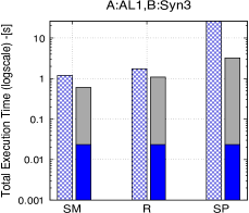
(a) P1.2

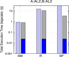
(b) P1.2

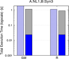
(c) P1.2

Figure 13. P1.2 evaluation time with and without rewriting

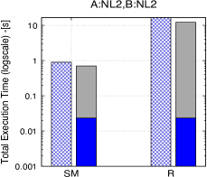
(a) P1.2

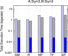
(b) P1.2

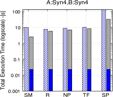
(c) P1.2

Figure 14. P1.2 evaluation time with and without rewriting

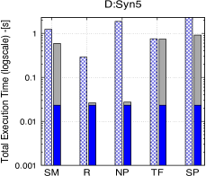
(a) P1.6

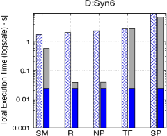
(b) P1.6

Figure 15. P1.6 evaluation time with and without rewriting

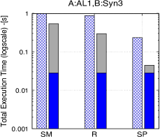
(a) P1.8

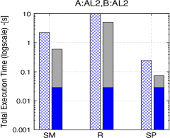
(b) P1.8

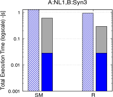
(c) P1.8

Figure 16. P1.8 evaluation time with and without rewriting

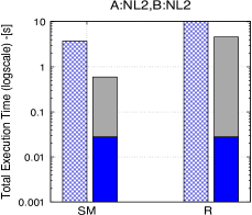
(a) P1.8

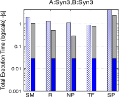
(b) P1.8

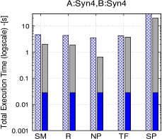
(c) P1.8

Figure 17. P1.8 evaluation time with and without rewriting

(a) P1.9

Figure 18. P1.9 evaluation time with and without rewriting

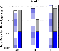
(a) P1.10

(b) P1.10

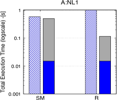
(c) P1.10

Figure 19. P1.10 evaluation time with and without rewriting

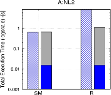
(a) P1.10

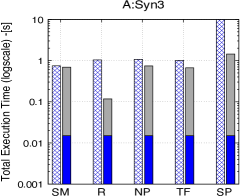
(b) P1.10

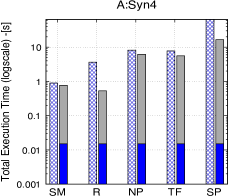
(c) P1.10

Figure 20. P1.10 evaluation time with and without rewriting

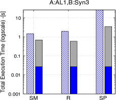
(a) P1.11

(b) P1.11

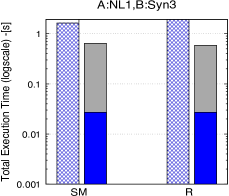
(c) P1.11

Figure 21. P1.11 evaluation time with and without rewriting

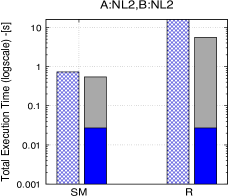
(a) P1.11

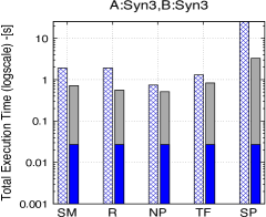
(b) P1.11

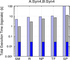
(c) P1.11

Figure 22. P1.11 evaluation time with and without rewriting

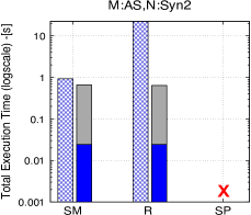
(a) P1.12

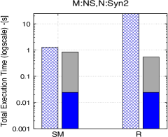
(b) P1.12

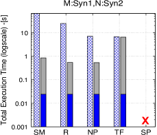
(c) P1.12

Figure 23. P1.12 evaluation time with and without rewriting

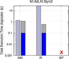
(a) P1.14

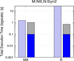
(b) P1.14

Figure 24. P1.14 evaluation time with and without rewriting

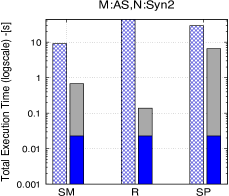
(a) P1.15

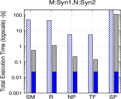
(b) P1.15

Figure 25. P1.15 evaluation time with and without rewriting

(a) P1.16

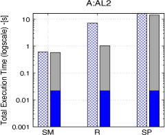
(b) P1.16

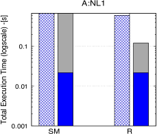
(c) P1.16

Figure 26. P1.16 evaluation time with and without rewriting

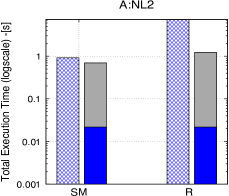
(a) P1.16

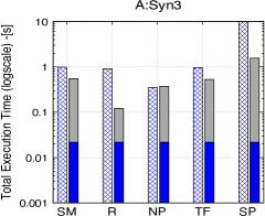
(b) P1.16

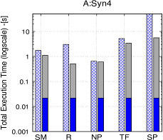
(c) P1.16

Figure 27. P1.16 evaluation time with and without rewriting

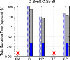
(a) P1.17

Figure 28. P1.17 evaluation time with and without rewriting

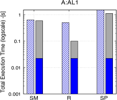
(a) P1.18

(b) P1.18

(c) P1.18

Figure 29. P1.18 evaluation time with and without rewriting

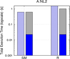
(a) P1.18

(b) P1.18

(c) P1.18

Figure 30. P1.18 evaluation time with and without rewriting

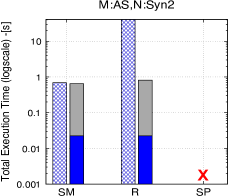
(a) P1.25

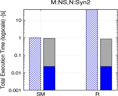
(b) P1.25

Figure 31. P1.25 evaluation time with and without rewriting

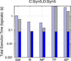
(a) P2.1

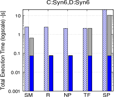
(b) P2.1

Figure 32. P2.1 evaluation time with and without rewriting

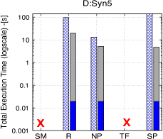
(a) P2.2

Figure 33. P2.2 evaluation time with and without rewriting

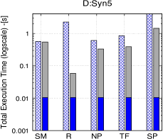
(a) P2.3

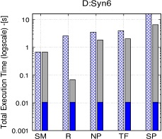
(b) P2.3

Figure 34. P2.3 evaluation time with and without rewriting

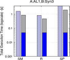
(a) P2.4

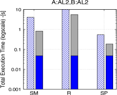
(b) P2.4

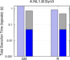
(c) P2.4

Figure 35. P2.4 evaluation time with and without rewriting

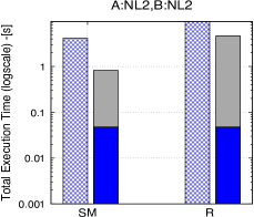
(a) P2.4

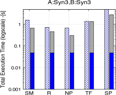
(b) P2.4

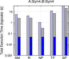
(c) P2.4

Figure 36. P2.4 evaluation time with and without rewriting

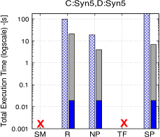
(a) P2.5

(b) P2.6

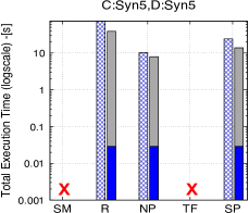
(c) P2.8

Figure 37. P2.5, P2.6 and P2.8 evaluation time with and without rewriting

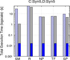
(a) P2.9

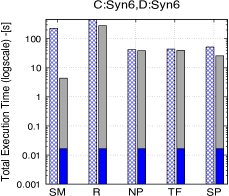
(b) P2.9S

Figure 38. P2.9 evaluation time with and without rewriting

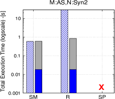
(a) P2.10

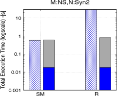
(b) P2.10

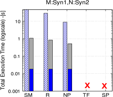
(c) P2.10

Figure 39. P2.10 evaluation time with and without rewriting

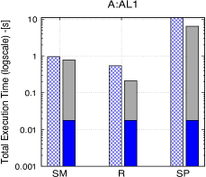
(a) P2.11

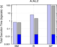
(b) P2.11

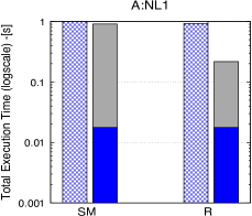
(c) P2.11

Figure 40. P2.11 evaluation time with and without rewriting

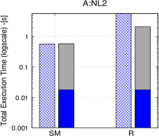
(a) P2.11

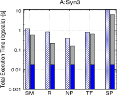
(b) P2.11

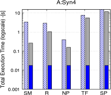
(c) P2.11

Figure 41. P2.11 evaluation time with and without rewriting

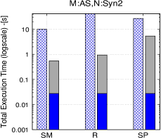
(a) P2.13

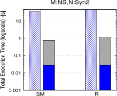
(b) P2.13

(c) P2.13

Figure 42. P2.13 evaluation time with and without rewriting

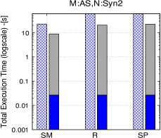
(a) P2.14

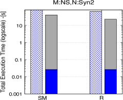
(b) P2.14

Figure 43. P2.14 evaluation time with and without rewriting

(a) P2.15

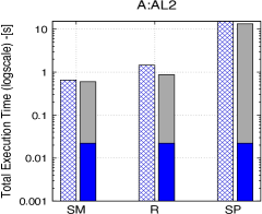
(b) P2.15

(c) P2.15

Figure 44. P2.15 evaluation time with and without rewriting

(a) P2.15

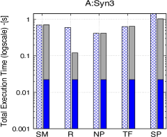
(b) P2.15

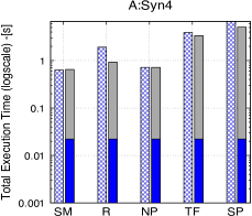
(c) P2.15

Figure 45. P2.15 evaluation time with and without rewriting

(a) P2.16

Figure 46. P2.16 evaluation time with and without rewriting

(a) P2.18

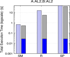
(b) P2.18

(c) P2.18

Figure 47. P2.18 evaluation time with and without rewriting

(a) P2.18

(b) P2.18

(c) P2.18

Figure 48. P2.18 evaluation time with and without rewriting

Appendix E Additional Results: $\mathcal{P}^{\neg Opt}$ Pipelines - MNC-based Cost Model

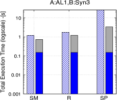
(a) P1.2

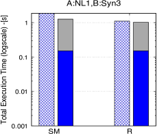
(b) P1.2

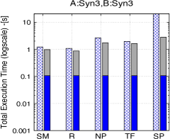
(c) P1.2

Figure 49. P1.2 evaluation time with and without rewriting

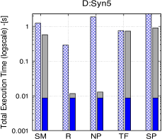
(a) P1.6

Figure 50. P1.6 evaluation time with and without rewriting

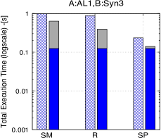
(a) P1.8

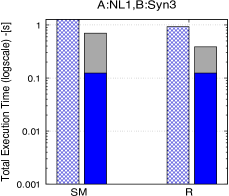
(b) P1.8

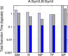
(c) P1.8

Figure 51. P1.8 evaluation time with and without rewriting

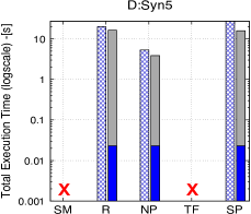
(a) P1.9

Figure 52. P1.9 evaluation time with and without rewriting

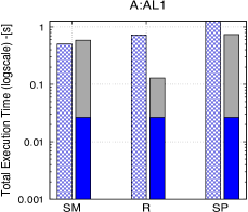
(a) P1.10

(b) P1.10

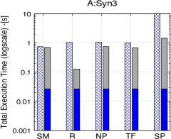
(c) P1.10

Figure 53. P1.10 evaluation time with and without rewriting

(a) P1.11

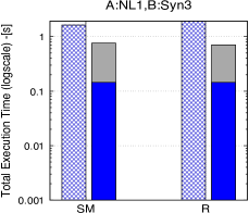
(b) P1.11

(c) P1.11

Figure 54. P1.11 evaluation time with and without rewriting

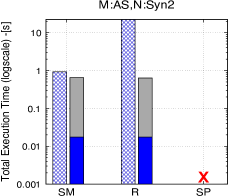
(a) P1.12

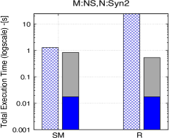
(b) P1.12

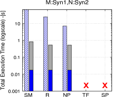
(c) P1.12

Figure 55. P1.12 evaluation time with and without rewriting

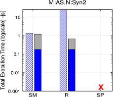
(a) P1.14

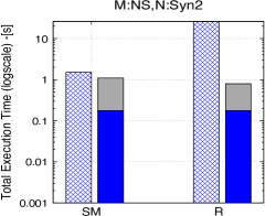
(b) P1.14

Figure 56. P1.14 evaluation time with and without rewriting

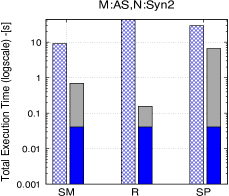
(a) P1.15

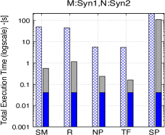
(b) P1.15

Figure 57. P1.15 evaluation time with and without rewriting

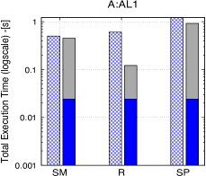
(a) P1.16

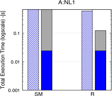
(b) P1.16

(c) P1.16

Figure 58. P1.16 evaluation time with and without rewriting

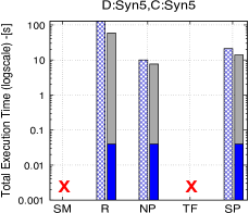
(a) P1.17

Figure 59. P1.17 evaluation time with and without rewriting

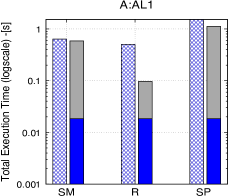
(a) P1.18

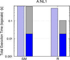
(b) P1.18

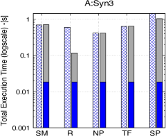
(c) P1.18

Figure 60. P1.18 evaluation time with and without rewriting

(a) P1.25

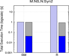
(b) P1.25

Figure 61. P1.25 evaluation time with and without rewriting

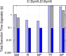
(a) P2.1

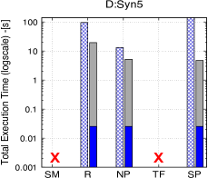
(b) P2.2

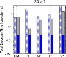
(c) P2.3

Figure 62. P2.1 evaluation time with and without rewriting

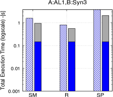
(a) P2.4

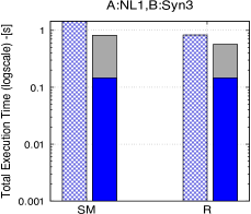
(b) P2.4

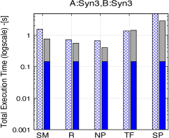
(c) P2.4

Figure 63. P2.4 evaluation time with and without rewriting

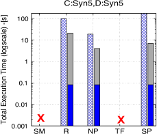
(a) P2.5

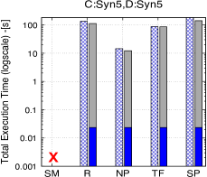
(b) P2.6

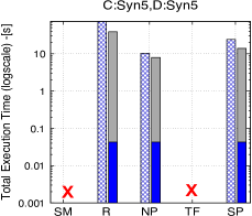
(c) P2.8

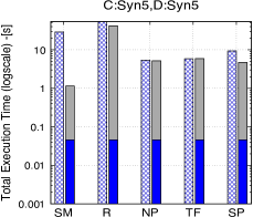
(d) P2.9

Figure 64. P2.5, P2.6, P2.8 and P2.9evaluation time with and without rewriting

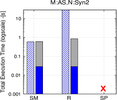
(a) P2.10

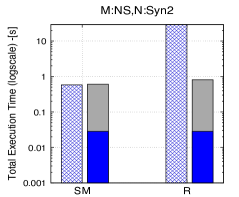
(b) P2.10

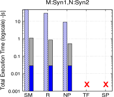
(c) P2.10

Figure 65. P2.10 evaluation time with and without rewriting

(a) P2.11

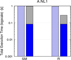
(b) P2.11

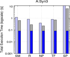
(c) P2.11

Figure 66. P2.11 evaluation time with and without rewriting

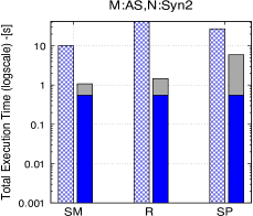
(a) P2.13

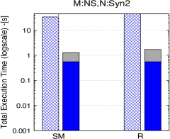
(b) P2.13

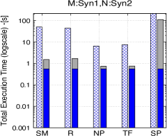
(c) P2.13

Figure 67. P2.13 evaluation time with and without rewriting

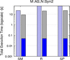
(a) P2.14

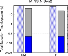
(b) P2.14

Figure 68. P2.14 evaluation time with and without rewriting

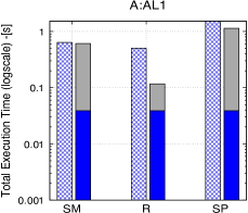
(a) P2.15

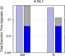
(b) P2.15

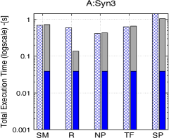
(c) P2.15

Figure 69. P2.15 evaluation time with and without rewriting

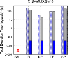
(a) P2.16

Figure 70. P2.16 evaluation time with and without rewriting

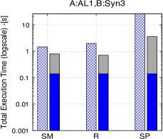
(a) P2.18

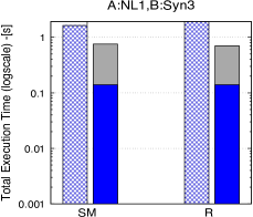
(b) P2.18

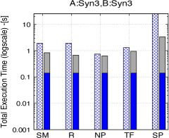
(c) P2.18

Figure 71. P2.18 evaluation time with and without rewriting

Appendix F Additional Results: $\mathcal{P}^{Views}$ Pipelines

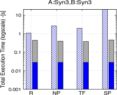
(a) P1.2

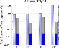
(b) P1.2

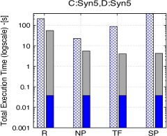
(c) P1.3

Figure 72. P1.2 and P1.3 evaluation time with and without rewriting

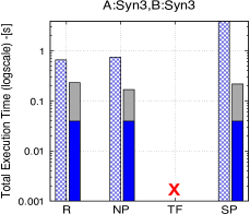
(a) P1.4

(b) P1.4

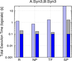
(c) P1.11

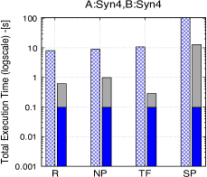
(d) P1.11

Figure 73. P1.4 and P1.11 evaluation time with and without rewriting

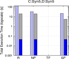
(a) P1.17

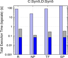
(b) P1.19

(c) P1.20

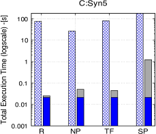
(d) P1.21

Figure 74. P1.17,P1.19,P1.20 and P1.21 evaluation time with and without rewriting

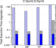
(a) P1.22

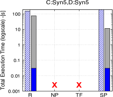
(b) P1.23

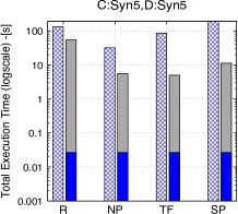
(c) P1.24

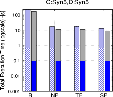
(d) P1.29

Figure 75. P1.22,P1.23,P1.24 and P1.29 evaluation time with and without rewriting

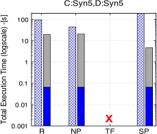
(a) P2.2

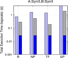
(b) P2.4

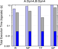
(c) P2.4

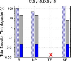
(d) P2.5

Figure 76. P2.2,P2.4 and P2.5 evaluation time with and without rewriting

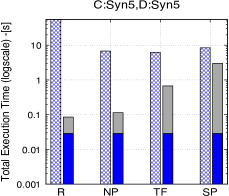
(a) P2.9

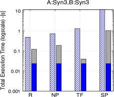
(b) P2.11

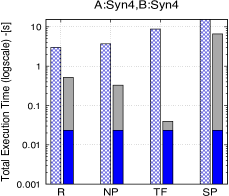
(c) P2.11

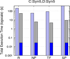
(d) P2.16

Figure 77. P2.9,P2.11 and P2.16 evaluation time with and without rewriting

Appendix G Hybrid Twitter Benchmark Queries and Views

⬇

import scala.math._

import org.apache.sysml.api.mlcontext._

import org.apache.sysml.api.mlcontext.ScriptFactory._

import org.apache.sysml.api.mlcontext.MatrixFormat._

import org.apache.spark.SparkContext

import org.apache.spark.SparkContext._

import org.apache.spark.SparkConf

import org.apache.spark.sql._

import scala.io.Source

import scala.tools.nsc.io._

import scala.collection.immutable._

import org.apache.spark.storage.StorageLevel._

//Preprocessing M

val sqlContext = new org.apache.spark.sql.SQLContext(sc)

val User = sqlContext.read.format("csv").option("header", "true").load("User.csv");

User.createOrReplaceTempView("User")

val Tweet = sqlContext.read.format("csv").option("header", "true").load("Tweet.csv");

Tweet.createOrReplaceTempView("Tweet")

val M = spark.sql("""SELECT followers_count,friends_count, listed_count,protected,verified

favorite_count,quote_count, reply_count,retweet_count,favorited,

possibly_sensitive,retweeted

FROM User as U, Tweet as T

WHERE T.id = U.id""")

constructMatirx (M2,"M.csv");

//Preprocessing (N)

val TweetJSON = spark.read.json("tweets/")

TweetJSON.createOrReplaceTempView("TweetJSON")

val N = spark.sql("""SELECT TJ.id, hID, TJ.filter_level

FROM TweetJSON AS TJ

LATERAL VIEW EXPLOD (entities.hashtags.id) AS hID

WHERE text LIKE ’%covid%’ AND

TJ.place.country_code =’US’""")

constructMTXMatirx (2380000,1000,N,"N.mtx");

//Analysis

val ml = new MLContext(spark)

ml.setConfigProperty("sysml.cp.parallel.ops","true")

ml.setConfigProperty("sysml.optlevel","4")

ml.setConfigProperty("sysml.localtmpdir","systemml")

//DML Query

val dmlTextQuery =

s"""

| M = read("M.csv", format="csv", header=FALSE, sep=",");

| N = readMM("N.mtx");

| V1 = read("V1.csv", format="csv", header=FALSE, sep=",");

| U1 = read("U1.csv", format="csv", header=FALSE, sep=",");

| X = read("X.csv", format="csv", header=FALSE, sep=",");

| NF = ifelse(N<=4,N,0)

| print(as.scalar(NF[20000,400]))

| res =rowSums(X%*%M) + (((U1%*%t(V1) ) + t(NF))%*%V1)

| while(FALSE){}

| print(as.scalar(res[500,1]))

| }

""".stripMargin

val dmlScript = dml(dmlTextQuery)

val result = ml.execute(dmlScript)

Listing G.1: Q1

⬇

import scala.math._

import org.apache.sysml.api.mlcontext._

import org.apache.sysml.api.mlcontext.ScriptFactory._

import org.apache.sysml.api.mlcontext.MatrixFormat._

import org.apache.spark.SparkContext

import org.apache.spark.SparkContext._

import org.apache.spark.SparkConf

import org.apache.spark.sql._

import scala.io.Source

import scala.tools.nsc.io._

import scala.collection.immutable._

import org.apache.spark.storage.StorageLevel._

//Preprocessing M

val sqlContext = new org.apache.spark.sql.SQLContext(sc)

val User = sqlContext.read.format("csv").option("header", "true").load("User.csv");

User.createOrReplaceTempView("User")

val Tweet = sqlContext.read.format("csv").option("header", "true").load("Tweet.csv");

Tweet.createOrReplaceTempView("Tweet")

val M = spark.sql("""SELECT followers_count,friends_count, listed_count,protected,verified

favorite_count,quote_count, reply_count,retweet_count,favorited,

possibly_sensitive,retweeted

FROM User as U, Tweet as T

WHERE T.id = U.id""")

constructMatirx (M2,"M.csv");

//Preprocessing (N)

val TweetJSON = spark.read.json("tweets/")

TweetJSON.createOrReplaceTempView("TweetJSON")

val N = spark.sql("""SELECT TJ.id, hID, TJ.filter_level

FROM TweetJSON AS TJ

LATERAL VIEW EXPLOD (entities.hashtags.id) AS hID

WHERE text LIKE ’%covid%’ AND

TJ.place.country_code =’US’""")

constructMTXMatirx (2380000,1000,N,"N.mtx");

//Analysis

val ml = new MLContext(spark)

ml.setConfigProperty("sysml.cp.parallel.ops","true")

ml.setConfigProperty("sysml.optlevel","4")

ml.setConfigProperty("sysml.localtmpdir","systemml")

//DML Query

val dmlTextQuery =

s"""

| M = read("M.csv", format="csv", header=FALSE, sep=",")

| N = readMM("N.mtx")

| X = read("X.csv", format="csv", header=FALSE, sep=",");

| U = read("U.csv", format="csv", header=FALSE, sep=",");

| NF = ifelse(N<=4,N,0)

| print(as.scalar(NF[20000,400]))

| res =U%*%colSums(t(X%*%M))+NF

| while(FALSE){}

| print(as.scalar(res[1,80]))

| }

""".stripMargin

val dmlScript = dml(dmlTextQuery)

val result = ml.execute(dmlScript)

Listing G.2: Q2

⬇

import scala.math._

import org.apache.sysml.api.mlcontext._

import org.apache.sysml.api.mlcontext.ScriptFactory._

import org.apache.sysml.api.mlcontext.MatrixFormat._

import org.apache.spark.SparkContext

import org.apache.spark.SparkContext._

import org.apache.spark.SparkConf

import org.apache.spark.sql._

import scala.io.Source

import scala.tools.nsc.io._

import scala.collection.immutable._

import org.apache.spark.storage.StorageLevel._

//Preprocessing M

val sqlContext = new org.apache.spark.sql.SQLContext(sc)

val User = sqlContext.read.format("csv").option("header", "true").load("User.csv");

User.createOrReplaceTempView("User")

val Tweet = sqlContext.read.format("csv").option("header", "true").load("Tweet.csv");

Tweet.createOrReplaceTempView("Tweet")

val M = spark.sql("""SELECT followers_count,friends_count, listed_count,protected,verified

favorite_count,quote_count, reply_count,retweet_count,favorited,

possibly_sensitive,retweeted

FROM User as U, Tweet as T

WHERE T.id = U.id""")

constructMatirx (M2,"M.csv");

//Preprocessing (N)

val TweetJSON = spark.read.json("tweets/")

TweetJSON.createOrReplaceTempView("TweetJSON")

val N = spark.sql("""SELECT TJ.id, hID, TJ.filter_level

FROM TweetJSON AS TJ

LATERAL VIEW EXPLOD (entities.hashtags.id) AS hID

WHERE text LIKE ’%covid%’ AND

TJ.place.country_code =’US’""")

constructMTXMatirx (2380000,1000,N,"N.mtx");

//Analysis

val ml = new MLContext(spark)

ml.setConfigProperty("sysml.cp.parallel.ops","true")

ml.setConfigProperty("sysml.optlevel","4")

ml.setConfigProperty("sysml.localtmpdir","systemml")

//DML Query

val dmlTextQuery =

s"""

| M = read("M.csv", format="csv", header=FALSE, sep=",");

| N = readMM("N.mtx");

| X = read("X.csv", format="csv", header=FALSE, sep=",");

| V = read("V.csv", format="csv", header=FALSE, sep=",");

| NF = ifelse(N<=4,N,0)

| print(as.scalar(NF[20000,400]))

| res = ((NF+X)%*%V)%*% colSums(M)

| while(FALSE){}

| print(as.scalar(res[500,1]))

| }

""".stripMargin

val dmlScript = dml(dmlTextQuery)

val result = ml.execute(dmlScript)

Listing G.3: Q3

⬇

import scala.math._

import org.apache.sysml.api.mlcontext._

import org.apache.sysml.api.mlcontext.ScriptFactory._

import org.apache.sysml.api.mlcontext.MatrixFormat._

import org.apache.spark.SparkContext

import org.apache.spark.SparkContext._

import org.apache.spark.SparkConf

import org.apache.spark.sql._

import scala.io.Source

import scala.tools.nsc.io._

import scala.collection.immutable._

import org.apache.spark.storage.StorageLevel._

//Preprocessing M

val sqlContext = new org.apache.spark.sql.SQLContext(sc)

val User = sqlContext.read.format("csv").option("header", "true").load("User.csv");

User.createOrReplaceTempView("User")

val Tweet = sqlContext.read.format("csv").option("header", "true").load("Tweet.csv");

Tweet.createOrReplaceTempView("Tweet")

val M = spark.sql("""SELECT followers_count,friends_count, listed_count,protected,verified

favorite_count,quote_count, reply_count,retweet_count,favorited,

possibly_sensitive,retweeted

FROM User as U, Tweet as T

WHERE T.id = U.id""")

constructMatirx (M2,"M.csv");

//Preprocessing (N)

val TweetJSON = spark.read.json("tweets/")

TweetJSON.createOrReplaceTempView("TweetJSON")

val N = spark.sql("""SELECT TJ.id, hID, TJ.filter_level

FROM TweetJSON AS TJ

LATERAL VIEW EXPLOD (entities.hashtags.id) AS hID

WHERE text LIKE ’%covid%’ AND

TJ.place.country_code =’US’""")

constructMTXMatirx (2380000,1000,N,"N.mtx");

//Analysis

val ml = new MLContext(spark)

ml.setConfigProperty("sysml.cp.parallel.ops","true")

ml.setConfigProperty("sysml.optlevel","4")

ml.setConfigProperty("sysml.localtmpdir","systemml")

//DML Query

val dmlTextQuery =

s"""

| M = read("M.csv", format="csv", header=FALSE, sep=",")

| N = readMM("N.mtx")

| X = read("X.csv", format="csv", header=FALSE, sep=",");

| U = read("U.csv", format="csv", header=FALSE, sep=",");

| v = read("v.csv", format="csv", header=FALSE, sep=",");

| NF = ifelse(N<=4,N,0)

| print(as.scalar(NF[20000,400]))

| res = sum(U+NF%*%colSums(X%*%M)%*%v)

| while(FALSE){}

| print(res)

| }

""".stripMargin

val dmlScript = dml(dmlTextQuery)

val result = ml.execute(dmlScript)

Listing G.4: Q4

⬇

import scala.math._

import org.apache.sysml.api.mlcontext._

import org.apache.sysml.api.mlcontext.ScriptFactory._

import org.apache.sysml.api.mlcontext.MatrixFormat._

import org.apache.spark.SparkContext

import org.apache.spark.SparkContext._

import org.apache.spark.SparkConf

import org.apache.spark.sql._

import scala.io.Source

import scala.tools.nsc.io._

import scala.collection.immutable._

import org.apache.spark.storage.StorageLevel._

//Preprocessing M

val sqlContext = new org.apache.spark.sql.SQLContext(sc)

val User = sqlContext.read.format("csv").option("header", "true").load("User.csv");

User.createOrReplaceTempView("User")

val Tweet = sqlContext.read.format("csv").option("header", "true").load("Tweet.csv");

Tweet.createOrReplaceTempView("Tweet")

val M = spark.sql("""SELECT followers_count,friends_count, listed_count,protected,verified

favorite_count,quote_count, reply_count,retweet_count,favorited,

possibly_sensitive,retweeted

FROM User as U, Tweet as T

WHERE T.id = U.id""")

constructMatirx (M2,"M.csv");

//Preprocessing (N)

val TweetJSON = spark.read.json("tweets/")

TweetJSON.createOrReplaceTempView("TweetJSON")

val N = spark.sql("""SELECT TJ.id, hID, TJ.filter_level

FROM TweetJSON AS TJ

LATERAL VIEW EXPLOD (entities.hashtags.id) AS hID

WHERE text LIKE ’%covid%’ AND

TJ.place.country_code =’US’""")

constructMTXMatirx (2380000,1000,N,"N.mtx");

//Analysis

val ml = new MLContext(spark)

ml.setConfigProperty("sysml.cp.parallel.ops","true")

ml.setConfigProperty("sysml.optlevel","4")

ml.setConfigProperty("sysml.localtmpdir","systemml")

//DML Query

val dmlTextQuery =

s"""

| M = read("M.csv", format="csv", header=FALSE, sep=",")

| N = readMM("N.mtx")

| U = read("U.csv", format="csv", header=FALSE, sep=",");

| X = read("X.csv", format="csv", header=FALSE, sep=",");

| NF = ifelse(N<=4,N,0)

| print(as.scalar(NF[20000,400]))

| res = U%*%colSums(M%*%X) + NF

| while(FALSE){}

| print(res)

| }

""".stripMargin

val dmlScript = dml(dmlTextQuery)

val result = ml.execute(dmlScript)

Listing G.5: Q5

⬇

import scala.math._

import org.apache.sysml.api.mlcontext._

import org.apache.sysml.api.mlcontext.ScriptFactory._

import org.apache.sysml.api.mlcontext.MatrixFormat._

import org.apache.spark.SparkContext

import org.apache.spark.SparkContext._

import org.apache.spark.SparkConf

import org.apache.spark.sql._

import scala.io.Source

import scala.tools.nsc.io._

import scala.collection.immutable._

import org.apache.spark.storage.StorageLevel._

//Preprocessing M

val sqlContext = new org.apache.spark.sql.SQLContext(sc)

val User = sqlContext.read.format("csv").option("header", "true").load("User.csv");

User.createOrReplaceTempView("User")

val Tweet = sqlContext.read.format("csv").option("header", "true").load("Tweet.csv");

Tweet.createOrReplaceTempView("Tweet")

val M = spark.sql("""SELECT followers_count,friends_count, listed_count,protected,verified

favorite_count,quote_count, reply_count,retweet_count,favorited,

possibly_sensitive,retweeted

FROM User as U, Tweet as T

WHERE T.id = U.id""")

constructMatirx (M2,"M.csv");

//Preprocessing (N)

val TweetJSON = spark.read.json("tweets/")

TweetJSON.createOrReplaceTempView("TweetJSON")

val N = spark.sql("""SELECT TJ.id, hID, TJ.filter_level

FROM TweetJSON AS TJ

LATERAL VIEW EXPLOD (entities.hashtags.id) AS hID

WHERE text LIKE ’%covid%’ AND

TJ.place.country_code =’US’""")

constructMTXMatirx (2380000,1000,N,"N.mtx");

//Analysis

val ml = new MLContext(spark)

ml.setConfigProperty("sysml.cp.parallel.ops","true")

ml.setConfigProperty("sysml.optlevel","4")

ml.setConfigProperty("sysml.localtmpdir","systemml")

//DML Query

val dmlTextQuery =

s"""

| M = read("M.csv", format="csv", header=FALSE, sep=",");

| N = readMM("N.mtx");

| V1 = read("V1.csv", format="csv", header=FALSE, sep=",");

| U1 = read("U1.csv", format="csv", header=FALSE, sep=",");

| X = read("X.csv", format="csv", header=FALSE, sep=",");

| NF = ifelse(N<=4,N,0)

| print(as.scalar(NF[20000,400]))

| res = rowSums(t(M%*%X)) + (((U1%*%t(V1) ) + NF)%*%V1)

| while(FALSE){}

| print(res[1000,1])

| }

""".stripMargin

val dmlScript = dml(dmlTextQuery)

val result = ml.execute(dmlScript)

Listing G.6: Q6

⬇

import scala.math._

import org.apache.sysml.api.mlcontext._

import org.apache.sysml.api.mlcontext.ScriptFactory._

import org.apache.sysml.api.mlcontext.MatrixFormat._

import org.apache.spark.SparkContext

import org.apache.spark.SparkContext._

import org.apache.spark.SparkConf

import org.apache.spark.sql._

import scala.io.Source

import scala.tools.nsc.io._

import scala.collection.immutable._

import org.apache.spark.storage.StorageLevel._

//Preprocessing M

val sqlContext = new org.apache.spark.sql.SQLContext(sc)

val User = sqlContext.read.format("csv").option("header", "true").load("User.csv");

User.createOrReplaceTempView("User")

val Tweet = sqlContext.read.format("csv").option("header", "true").load("Tweet.csv");

Tweet.createOrReplaceTempView("Tweet")

val M = spark.sql("""SELECT followers_count,friends_count, listed_count,protected,verified

favorite_count,quote_count, reply_count,retweet_count,favorited,

possibly_sensitive,retweeted

FROM User as U, Tweet as T

WHERE T.id = U.id""")

constructMatirx (M2,"M.csv");

//Preprocessing (N)

val TweetJSON = spark.read.json("tweets/")

TweetJSON.createOrReplaceTempView("TweetJSON")

val N = spark.sql("""SELECT TJ.id, hID, TJ.filter_level

FROM TweetJSON AS TJ

LATERAL VIEW EXPLOD (entities.hashtags.id) AS hID

WHERE text LIKE ’%covid%’ AND

TJ.place.country_code =’US’""")

constructMTXMatirx (2380000,1000,N,"N.mtx");

//Analysis

val ml = new MLContext(spark)

ml.setConfigProperty("sysml.cp.parallel.ops","true")

ml.setConfigProperty("sysml.optlevel","4")

ml.setConfigProperty("sysml.localtmpdir","systemml")

//DML Query

val dmlTextQuery =

s"""

| M = read("M.csv", format="csv", header=FALSE, sep=",")

| N = readMM("N.mtx")

| X = read("X.csv", format="csv", header=FALSE, sep=",");

| U = read("U,csv", format="csv", header=FALSE, sep=",");

| NF = ifelse(N<=4,N,0)

| print(as.scalar(NF[20000,400]))

| res= X%*%NF%*%U + rowSums(t(M))

| while(FALSE){}

| print(res[2,30])

| }

""".stripMargin

val dmlScript = dml(dmlTextQuery)

val result = ml.execute(dmlScript)

Listing G.7: Q7

⬇

import scala.math._

import org.apache.sysml.api.mlcontext._

import org.apache.sysml.api.mlcontext.ScriptFactory._

import org.apache.sysml.api.mlcontext.MatrixFormat._

import org.apache.spark.SparkContext

import org.apache.spark.SparkContext._

import org.apache.spark.SparkConf

import org.apache.spark.sql._

import scala.io.Source

import scala.tools.nsc.io._

import scala.collection.immutable._

import org.apache.spark.storage.StorageLevel._

//Preprocessing M

val sqlContext = new org.apache.spark.sql.SQLContext(sc)

val User = sqlContext.read.format("csv").option("header", "true").load("User.csv");

User.createOrReplaceTempView("User")

val Tweet = sqlContext.read.format("csv").option("header", "true").load("Tweet.csv");

Tweet.createOrReplaceTempView("Tweet")

val M = spark.sql("""SELECT followers_count,friends_count, listed_count,protected,verified

favorite_count,quote_count, reply_count,retweet_count,favorited,

possibly_sensitive,retweeted

FROM User as U, Tweet as T

WHERE T.id = U.id""")

constructMatirx (M2,"M.csv");

//Preprocessing (N)

val TweetJSON = spark.read.json("tweets/")

TweetJSON.createOrReplaceTempView("TweetJSON")

val N = spark.sql("""SELECT TJ.id, hID, TJ.filter_level

FROM TweetJSON AS TJ

LATERAL VIEW EXPLOD (entities.hashtags.id) AS hID

WHERE text LIKE ’%covid%’ AND

TJ.place.country_code =’US’""")

constructMTXMatirx (2380000,1000,N,"N.mtx");

//Analysis

val ml = new MLContext(spark)

ml.setConfigProperty("sysml.cp.parallel.ops","true")

ml.setConfigProperty("sysml.optlevel","4")

ml.setConfigProperty("sysml.localtmpdir","systemml")

//DML Query

val dmlTextQuery =

s"""

| M = read("M.csv", format="csv", header=FALSE, sep=",")

| N = readMM("N.mtx")

| C = read("C.csv", format="csv", header=FALSE, sep=",");

| V = read("V.csv", format="csv", header=FALSE, sep=",");

| X = read("X.csv", format="csv", header=FALSE, sep=",");

| NF = ifelse(N<=4,N,0)

| print(as.scalar(NF[20000,400]))

| res = NF*trace(C+ V%*%colSums(M%*%X)%*%C)

| while(FALSE){}

| print(res[2,30])

| }

""".stripMargin

val dmlScript = dml(dmlTextQuery)

val result = ml.execute(dmlScript)

Listing G.8: Q8

⬇

import scala.math._

import org.apache.sysml.api.mlcontext._

import org.apache.sysml.api.mlcontext.ScriptFactory._

import org.apache.sysml.api.mlcontext.MatrixFormat._

import org.apache.spark.SparkContext

import org.apache.spark.SparkContext._

import org.apache.spark.SparkConf

import org.apache.spark.sql._

import scala.io.Source

import scala.tools.nsc.io._

import scala.collection.immutable._

import org.apache.spark.storage.StorageLevel._

//Preprocessing M

val sqlContext = new org.apache.spark.sql.SQLContext(sc)

val User = sqlContext.read.format("csv").option("header", "true").load("User.csv");

User.createOrReplaceTempView("User")

val Tweet = sqlContext.read.format("csv").option("header", "true").load("Tweet.csv");

Tweet.createOrReplaceTempView("Tweet")

val M = spark.sql("""SELECT followers_count,friends_count, listed_count,protected,verified

favorite_count,quote_count, reply_count,retweet_count,favorited,

possibly_sensitive,retweeted

FROM User as U, Tweet as T

WHERE T.id = U.id""")

constructMatirx (M2,"M.csv");

//Preprocessing (N)

val TweetJSON = spark.read.json("tweets/")

TweetJSON.createOrReplaceTempView("TweetJSON")

val N = spark.sql("""SELECT TJ.id, hID, TJ.filter_level

FROM TweetJSON AS TJ

LATERAL VIEW EXPLOD (entities.hashtags.id) AS hID

WHERE text LIKE ’%covid%’ AND

TJ.place.country_code =’US’""")

constructMTXMatirx (2380000,1000,N,"N.mtx");

//Analysis

val ml = new MLContext(spark)

ml.setConfigProperty("sysml.cp.parallel.ops","true")

ml.setConfigProperty("sysml.optlevel","4")

ml.setConfigProperty("sysml.localtmpdir","systemml")

//DML Query

val dmlTextQuery =

s"""

| M = read("M.csv", format="csv", header=FALSE, sep=",")

| N = readMM("N.mtx")

| C = read("C.csv", format="csv", header=FALSE, sep=",");

| X = read("X.csv", format="csv", header=FALSE, sep=",");

| NF = ifelse(N<=4,N,0)

| print(as.scalar(NF[20000,400]))

| res = X*sum(t(colSums(C)*rowSums(M))+NF

| while(FALSE){}

| print(res[2,30])

| }

""".stripMargin

val dmlScript = dml(dmlTextQuery)

val result = ml.execute(dmlScript)

Listing G.9: Q9

⬇

import scala.math._

import org.apache.sysml.api.mlcontext._

import org.apache.sysml.api.mlcontext.ScriptFactory._

import org.apache.sysml.api.mlcontext.MatrixFormat._

import org.apache.spark.SparkContext

import org.apache.spark.SparkContext._

import org.apache.spark.SparkConf

import org.apache.spark.sql._

import scala.io.Source

import scala.tools.nsc.io._

import scala.collection.immutable._

import org.apache.spark.storage.StorageLevel._

//Preprocessing M

val sqlContext = new org.apache.spark.sql.SQLContext(sc)

val User = sqlContext.read.format("csv").option("header", "true").load("User.csv");

User.createOrReplaceTempView("User")

val Tweet = sqlContext.read.format("csv").option("header", "true").load("Tweet.csv");

Tweet.createOrReplaceTempView("Tweet")

val M = spark.sql("""SELECT followers_count,friends_count, listed_count,protected,verified

favorite_count,quote_count, reply_count,retweet_count,favorited,

possibly_sensitive,retweeted

FROM User as U, Tweet as T

WHERE T.id = U.id""")

constructMatirx (M2,"M.csv");

//Preprocessing (N)

val TweetJSON = spark.read.json("tweets/")

TweetJSON.createOrReplaceTempView("TweetJSON")

val N = spark.sql("""SELECT TJ.id, hID, TJ.filter_level

FROM TweetJSON AS TJ

LATERAL VIEW EXPLOD (entities.hashtags.id) AS hID

WHERE text LIKE ’%covid%’ AND

TJ.place.country_code =’US’""")

constructMTXMatirx (2380000,1000,N,"N.mtx");

//Analysis

val ml = new MLContext(spark)

ml.setConfigProperty("sysml.cp.parallel.ops","true")

ml.setConfigProperty("sysml.optlevel","4")

ml.setConfigProperty("sysml.localtmpdir","systemml")

//DML Query

val dmlTextQuery =

s"""

| M = read("M.csv", format="csv", header=FALSE, sep=",")

| N = readMM("N.mtx")

| C = read("C.csv", format="csv", header=FALSE, sep=",");

| X = read("X.csv", format="csv", header=FALSE, sep=",");

| NF = ifelse(N<=4,N,0)

| print(as.scalar(NF[20000,400]))

| res = NF*sum((X+C)%*%M)

| while(FALSE){}

| print(res[2,30])

| }

""".stripMargin

val dmlScript = dml(dmlTextQuery)

val result = ml.execute(dmlScript)

Listing G.10: Q10

⬇

T<-read.csv("Tweet.csv")

U<-read.csv("User.csv")

K <-sparseMatrix(i=1:nrow(U), j=T[,"id"], x=1)

T1 <- as.matrix(subset(T, select = c("favorite_count","quote_count","reply_count",

"retweet_count","favorited","possibly_sensitive","retweeted" )))

U1 <-as.matrix(subset(U, select = c("followers_count","friends_count", "listed_count","protected","verified" )))

V3<-rowSums(T1)+K%*%rowSums(U1)

write.csv(as.matrix(V3),"V3.csv", row.names = FALSE)

Listing G.11: V3

⬇

T<-read.csv("Tweet.csv")

U<-read.csv("User.csv")

K <-sparseMatrix(i=1:nrow(U), j=T[,"id"], x=1)

T1 <- as.matrix(subset(T, select = c("favorite_count","quote_count","reply_count",

"retweet_count","favorited","possibly_sensitive","retweeted" )))

U1 <-as.matrix(subset(U, select = c("followers_count","friends_count", "listed_count","protected","verified" )))

V4<-cbind(colSums(T1),colSums(K)%*%U1)

write.csv(as.matrix(V4),"V4.csv", row.names = FALSE)

Listing G.12: V4

⬇

T<-read.csv("Tweet.csv")

U<-read.csv("User.csv")

C<-read.csv("C.csv")

K <-sparseMatrix(i=1:nrow(U), j=T[,"id"], x=1)

T1 <- as.matrix(subset(T, select = c("favorite_count","quote_count","reply_count",

"retweet_count","favorited","possibly_sensitive","retweeted" )))

U1 <-as.matrix(subset(U, select = c("followers_count","friends_count", "listed_count","protected","verified" )))

V4<-cbind(C%*%T1,(C%*%K)%*%U1)

write.csv(as.matrix(V5),"V5.csv", row.names = FALSE)

Listing G.13: V5