Different Environmental Conditions in Genetic Algorithm

Abstract

We propose an extended genetic algorithm (GA) with different local environmental conditions. Genetic entities, or configurations, are put on nodes in a ring structure, and location-dependent environmental conditions are applied for each entity. Our GA is motivated by the geographic aspect of natural evolution: Geographic isolation reduces the diversity in a local group, but at the same time, can enhance intergroup diversity. Mating of genetic entities across different environments can make it possible to search for broad area of the fitness landscape. We validate our extended GA for finding the ground state of three-dimensional spin-glass system and find that the use of different environmental conditions makes it possible to find the lower-energy spin configurations at relatively shorter computation time. Our extension of GA belongs to a meta-optimization method and thus can be applied for a broad research area in which finding of the optimal state in a shorter computation time is the key problem.

1 Introduction

Genetic algorithm (GA) has been proposed by John H. Holland in 1975 [1], and has become a well-adopted technique in various research areas to solve computationally difficult problems [2]. In the process of Darwinian evolution, various mechanisms of genetic mutations produce offsprings of different fitness, and the fitter tend to survive and produce more offsprings later on. Likewise, GA in various optimization problems first produces a group of candidate solutions, and only a part of them are then selected to become parent solutions to next generation.

In the most basic scheme of GA, each of possible solutions to the target problem is encoded as a genotypic entity or a configuration, and a set of initial genotype populations are generated randomly and ranked in terms of the fitness, a specific variable which denotes how well the individual suits the conditions of the target problem. Each individual entity has a chance to mate with another entity and to produce offsprings, whose genetic traits are inherited from parents. The entity with a high fitness is set to be advantageous and the system as a whole tends to approach the desired optimum with the highest fitness value. It is a widespread observation that GA can locate efficiently an approximate solution of a given complex problem in a relatively short time [3, 4, 5].

However, despite of its usefulness, basic GA has a few drawbacks which have to be resolved. For example, since genotypes of offspring entities are generated by the combination of genotypes of their parents, a simple GA system possesses a risk of losing genetic diversity and converging into only a few genotypes near a local maximum in the fitness landscape. Most of GA’s use the mutation process, which adds a random noise to genotypes of each offsprings, to maintain a certain level of the genetic diversity [6]. In the same spirit, many revised or extended mechanisms have been suggested to improve various aspect of GA’s: Wiriyasermkul et al. have proposed a meiosis GA, which imposes a duplication process to create two types of offsprings [7]. Sánchez-Velazco et al. assigned a gender attribute to the genetic entity and introduced the effect of asymmetric mating and reproduction process [8].

In the present paper, we propose an extension of GA which utilizes a geographic aspect of natural evolution [9, 10, 11]. Such geographic effect can be easily seen in the famous example of Darwin’s finches: Different species of finches evolved in different local environments. We are motivated by such well-known observation in nature, and propose that migrations and mating across different local environments can broaden the search space of the fitness landscape. Location-specific environment allows largely different genetic entities to survive in different local conditions and mating between genetic entities at separate locations can provide a larger diversity in a gene pool.

Our GA needs to be compared with the island model [12], in which genetic entities are distributed across islands. Although mating is allowed only within an island, islands are allowed to exchange genetic entities with each other, and thus successful offsprings can spread out. The island model as well as our GA in the present paper can be phrased as a meta-optimization algorithm since one can apply suggested methodology on top of the conventional optimization algorithm. In the island model, the frequency and the magnitude of the exchange across islands are tunable parameters for the meta-optimization, and our GA uses the difference in environmental conditions for that purpose. It has been reported that properly adjusted island model often outperforms the basic GA [13]. Likewise, we hope to optimize our modified GA with different environmental conditions to achieve better performance. We emphasize that the present work does not aim to get the best optimum for a given problem. Instead, we are trying to show that addition of different environmental conditions for a given optimization problem can be helpful in a practical sense to find a better optimum in a shorter computation time.

In our approach, genetic entities are organized into a specific network structure so that each of them can have a regional attribute. By applying heterogeneous environmental factors to a suitably defined fitness function, we are able to construct a genetic system which consists of individuals with different location-specific objectives. If each genetic entity is allowed to mate with a local or a remote partner, we are able to observe how environmental difference between parents affects the survivals of offsprings. It is to be noted that we use the geographic isolation in a positive way: Isolation makes each local group lose genetic diversity within the group, but at the same time, it can help each local group to have a genotype largely different from other local groups due to different environmental conditions. In other words, our GA with heterogeneous environmental factors reduces intragroup diversity but enhances intergroup diversity, and the latter is the main source of genetic diversity in our framework.

2 Method

In order to investigate the concrete effect of our GA, we use a specific physics problem of finding the ground state of the Edwards-Anderson spin-glass model [14] with an external field. we again emphasize that we are not seeking the lowest possible energy state of the model, but we hope to show that the use of the different environmental condition can effectively enhance the performance of GA in finding lower-energy state. The EA model has been widely used as an archetype to investigate complex collaborative glass behavior. The Hamiltonian of the EA model reads

$$\mathcal{H}=-\sum_{\langle ij\rangle}J_{ij}s_{i}s_{j}-h\sum_{i}s_{i},$$ (1)

where the sum $\sum_{\langle ij\rangle}$ runs only for nearest-neighbor pairs with the periodic boundary condition, $s_{i}(=\pm 1)$ is the Ising spin variable at the $i$th site, $J_{ij}$ is the coupling strength of the atomic bond between spins at the sites $i$ and $j$, and $h$ is the spatially uniform external field. Note that the local interaction structure makes it difficult to obtain the ground state of the system: It has been proven that finding the ground state of the EA model in three dimensions (3D) is NP-complete problem [15]. Of course, we can instead use a numerical approach to find the ground state, and several techniques, such as simulated annealing [16], population annealing [17], extremal optimization [18], genetic algorithm [19], and branch-and-cut algorithm [20] have been suggested and applied in previous researches. In particular, the branch-and-cut algorithm is known to find the exact ground state in shorter computation time[20]. Although it is challenging work to make better algorithm than existing ones designed for the specific problem, we rather focus on more general aspect of optimization problem. In the present work we aim to propose how one can enhance the performance of a genetic algorithm through the environment-driven genetic diversity with the 3D EA model as an exemplar system.

The basic scheme of our genetic algorithm starts from a ring network which consists of $M$ nodes as shown in Fig. 1. Each node represents a whole three-dimensional spin configuration of the linear size $L$ (and thus the total number $N$ of spins satisfies $N=L^{3}$), which is connected to two (left and right) neighbor nodes as in Fig. 1. The node index $a$ increases in the counterclockwise direction from 1 to $M$. Since nodes are arranged in the form of a ring, the distance between two nodes $a$ and $b$ is written as $\min(M-|a-b|,|a-b|)$, to impose the periodicity along the circular ring structure. To emphasize that a node in the ring represents a whole 3D spin-glass system, we call each node as a system node from now on.

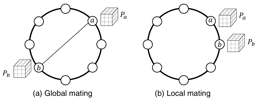
Figure 1: Schematic illustration of our genetic algorithm. A ring network of $M$ nodes is constructed, and a spin system is put on each node. In more general context, a node can represent a genetic entity that evolves in time. (a) Global mating: At the global mating probability $p$ we pick a node at $b(\neq a)$ completely at random among all other nodes in the ring network. (b) Local mating: with the probability $1-p$, one (at $b$) of $a$’s two nearest neighbors is randomly chosen. The two spin systems $P_{a}$ and $P_{b}$ at $a$ and $b$, respectively, mate and reproduce offsprings (see text).

The Hamiltonian of the system node $a$ is defined according to Eq. (1) as

$$\mathcal{H}^{a}(t)=-\sum_{\langle ij\rangle}J_{ij}s_{i}^{a}s_{j}^{a}-h^{a}(t)\sum_{i}s_{i}^{a},$$ (2)

where $s_{i}^{a}$ is the $i$-th spin of the system node $a$ and satisfies the periodic boundary condition ($s^{a}_{i+L\hat{x}}=s^{a}_{i+L\hat{y}}=s^{a}_{i+L\hat{z}}=s^{a}_{i}$ with $\hat{x}$, $\hat{y}$, and $\hat{z}$ being unit vectors in the 3D Cartesian coordinate system), and the coupling strength $J_{ij}$ is the quenched random variable generated from the Gaussian distribution with zero mean and unit variance. It is important to note that $\{J_{ij}\}$ is identical across system nodes, and thus all system nodes are assigned exactly the same optimization problem in the absence of the external field. The external field $h^{a}(t)$ explicitly depends on the node index $a$ and the time $t$, which is the key ingredient in our GA to mimic the different environmental condition in the evolution process. The time variable $t$ can be considered as an index for generation, to be explained more below.

In order to implement a geographically heterogeneous and time-varying environmental condition, the external field $h^{a}(t)$ with the amplitude $h_{0}$ is written as

$$h^{a}(t)=h_{0}\sin\left[2\pi\left(\frac{a}{M}-\frac{t}{T}\right)\right],$$ (3)

which is periodic both in spatial and temporal dimensions. The spatial periodicity $h^{a}(t)$ can be interpreted as, e.g., the change of environmental condition with the latitude on the earth, whereas the temporal periodicity of $h^{a}(t)$ can be interpreted as some long-term climate change like the periodic occurrences of ice ages on the earth. Since $h^{a}(t)$ oscillates in time around zero, each system node faces the same optimization problem in an average sense. Note that both parameters affect the fundamental dynamics of a genetic system and we use them as parameters in the meta-optimization scheme.

Our genetic algorithm in the present work can be roughly divided into five stages: (i) initialization, (ii) mating, (iii) crossover, (iv) mutation, and (v) competition. We describe each stage one by one in the followings.

1. Initialization: All spins at each system node in the ring network are randomly set to $1$ or $-1$ at equal probability.

2. Mating: We randomly pick a parent $P_{a}$ at the system node $a$. The other parent $P_{b}$ at the system node $b$ to mate with $P_{a}$ is chosen in either of the two ways: the global mating with the probability $p$ and the local mating with probability $1-p$ (see Fig. 1). For the former, $b$ is chosen at random among all other system nodes, while for the latter mating, $b$ is chosen between the two (the left and the right) neighbor nodes of $a$. Throughout the present work, we use the global mating probability $p=1/2$.

3. Crossover: Spins of two parents $P_{a}$ and $P_{b}$ are combined to create the first ($O_{1}$) and the second ($O_{2}$) offsprings whose spin configurations are written as $\{s_{i}^{O_{1}}\}$ and $\{s_{i}^{O_{2}}\}$, respectively, with $i=1,2,\cdots,N$. We assume that the crossover process is uniform across all spins, and thus there are only two possibilities for each spin at the $i$th site: $(s_{i}^{O_{1}}=s_{i}^{P_{a}},s_{i}^{O_{2}}=s_{i}^{P_{b}})$ or $(s_{i}^{O_{1}}=s_{i}^{P_{b}},s_{i}^{O_{2}}=s_{i}^{P_{a}})$ at equal probability of 1/2. Note that this crossover process we adopt here is the most basic one, and that there are other more advanced schemes [21].

4. Mutation: Each spin in the offspring configurations is reversed ($s_{i}^{O_{1}}\rightarrow-s_{i}^{O_{1}}$, $s_{i}^{O_{2}}\rightarrow-s_{i}^{O_{2}}$) at the mutation probability $\mu=0.01$. Although mutation process has often been utilized to provide a genetic diversity in most previous studies, it is not the only source of genetic diversity in our framework.

5. Competition: Once the spin configurations of two offsprings are constructed in (iv), we then decide where these offsprings are to be born. There are two possibilities: $O_{1}$ is at the system node $a$ and $O_{2}$ at $b$, and vice versa. In order to maintain the continuity of genetic system, we make a reasonable assumption that the local environmental condition at $a$ will be more friendly for an offspring who has a spin configuration closer to the parent at $a$. We use the Hamming distance $D(\alpha,\beta)\equiv\sum_{i}[1-\delta(s_{i}^{\alpha},s_{i}^{\beta})]$ with the Kronecker-$\delta$, to measure the similarity between two spin configurations $\alpha$ and $\beta$. We then compare $D(P_{a},O_{1})+D(P_{b},O_{2})$ and $D(P_{a},O_{2})+D(P_{b},O_{1})$: If the former is less than the latter, this can be interpreted as that $O_{1}$ and $O_{2}$ have spin configurations closer to those of parents at $a$ and $b$, and thus we decide that $O_{1}$ is born at $a$ and $O_{2}$ at $b$. Otherwise, if $D(P_{a},O_{1})+D(P_{b},O_{2})>D(P_{a},O_{2})+D(P_{b},O_{1})$, the situation is reversed and thus $O_{1}$ and $O_{2}$ are born at $b$ and $a$, respectively. At each location, we compute the energy values for the parent and the new born offspring, and the one with the lower energy is selected to survive there.

3 Results

In our simulations, the ring network (see Fig. 1) has the size $M=100$, and each system node consists of the 3D EA spin-glass model of the linear size $L=5$ (and thus total number of spins $N=L^{3}=125$). The two control parameters are the amplitude $h_{0}$ and the temporal period $T$ of the local magnetic field in Eq. (3) in our meta-optimization scheme.

We initialize the spin configuration of each system node in (i) Initialization step, and iterate the procedure (ii)-(v). We measure the time $t$ in such a way that steps (ii)-(v) are iterated once for each system node on average in one unit of time. In other words, $M(=100)$ repetitions of steps (ii)-(v) amount one unit of time. Simulations are stopped at $t=t_{\rm max}=5000$, which is long enough for most parameter values. We then repeat the above whole procedure 5000 times with different random configuration of $\{J_{ij}\}$ and averages are taken for these independent runs. In order to investigate the performance of our GA, we measure the minimum energy and average diversity at time $t$ defined by

$$E_{\rm min}(t)\equiv-\left\langle\min_{a}\frac{1}{N}\sum_{\langle ij\rangle}J_{ij}s_{i}^{a}(t)s_{j}^{a}(t)\right\rangle,$$ (4)

$$D_{\rm avg}(t)\equiv\left\langle\frac{1}{M(M-1)N}\sum_{b\neq a}\sum_{i}\Bigl{\{}1-\delta\bigl{[}s_{i}^{a}(t),s_{i}^{b}(t)\bigr{]}\Bigr{\}}\right\rangle,$$ (5)

where $\langle\cdots\rangle$ represents the ensemble average over iterations for 5000 different configurations of $\{J_{ij}\}$.

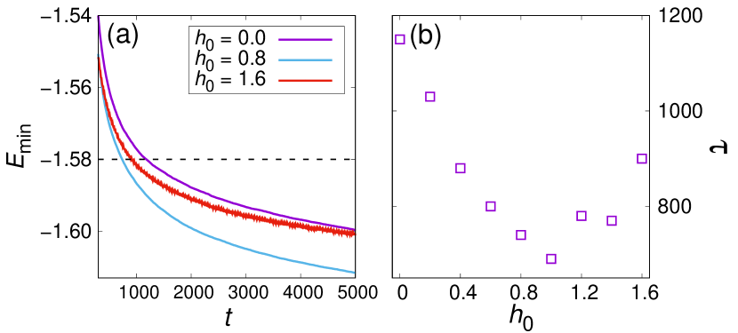
Figure 2: (a) The minimum energy $E_{\rm min}(t)$ at temporal period $T=50$, as a function of $t$ at the field strength $h_{0}$ = 0.0, 0.8, and 1.6. (b) The decay time scale $\tau$ defined by $E_{\rm min}(t=\tau)=-1.58$ [see the horizontal dashed line in (a)] exhibits minimum around $h_{0}=1.0$, which indicates that our GA performs better at the intermediate field strength and thus can find lower energy configuration in a relatively shorter computation time.

In Fig. 2, we display $E_{\rm min}(t)$ versus time $t$ for $t\in[300,5000]$ at $h_{0}=0.0,0.8$, and 1.6, and the time period is fixed at $T=50$. In Fig. 2(a), we first notice that in the absence of the external field ($h_{0}=0$), $E_{\rm min}(t)$ displays a relatively slow decay. At larger values of the field strength ($h_{0}=0.8$ and $1.6$), on the other hand, the minimum energy decrease faster in early time region. It is very interesting to observe in Fig. 2(a) that the decay of $E_{\rm min}(t)$ is faster at $h_{0}=0.8$ than at $h_{0}=0.0$ and $h_{0}=1.6$. This strongly suggests that our modified GA becomes more efficient at the intermediate field strength in finding the lower-energy state.

In order to check more carefully the nonmonotonic behavior observed in Fig. 2(a), we measure the decay time scale $\tau$ at which $E_{\rm min}=-1.58$ is crossed, as represented by the horizontal dashed line in Fig. 2(a). The smaller $\tau$ is, the faster our GA approaches a lower-energy state. Figure 2(b) exhibits the decay time $\tau$ as a function of the field strength $h_{0}$ at $T=50$, which clearly shows the expected non-monotonic behavior. We thus conclude that the use of the proper strength of the heterogeneous field reflecting the different environmental condition can make our GA more efficient.

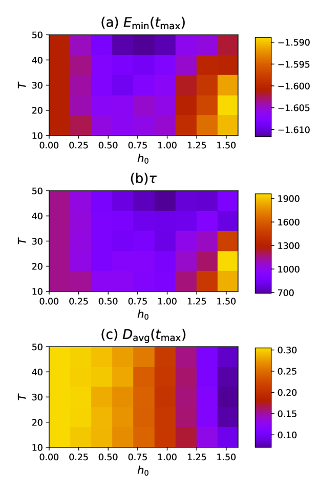
Figure 3: (a) The minimum energy $E_{\rm min}(t_{\rm max})$, (b) the decay time $\tau$ defined by $E_{\rm min}(t=\tau)=-1.58$, and (c) the genetic diversity $D_{\rm avg}(t_{\rm max})$, with $t_{\rm max}=5000$ in the plane of ($h_{0}$,$T$). Note that the use of the field strength e.g., $h_{0}\approx 0.8$ and the temporal period $T\approx 50$ can achieve a lower energy [see (a)] in a shorter computation time [see (b)] with preserving an appropriate level of genetic diversity [see (c)].

Figure 3 displays the performance of our GA at various values of $h_{0}$ and $T$. We first notice that $E_{\rm min}(t_{\rm max}=5000)$ in Fig. 3(a) exhibits a minimum around $h_{0}\approx 0.8$ and $T\approx 50$. As can be seen in Fig. 2(a), the system may not have approached a steady state till $t=5000$. However, we limit the simulation time up to $t_{\rm max}=5000$, to focus on practical applicability of our method: We aim to find low enough energy state for a given limitation of simulation time. As was already seen in Fig. 2(a), the observation implies that a certain level of inhomogeneity in the environmental condition is beneficial in finding the lower-energy state.

The behavior of the decay time $\tau$ in Fig. 3(b) also shows a similar tendency: The minimum occurs at $h_{0}\approx 1.0$ and $T\approx 50$. In addition, the genetic diversity $D_{\rm avg}(t_{\rm max})$ measured at $t=t_{\rm max}$ in Fig. 3(c) provides a validity of above results. Although the system loses its diversity as $h_{0}$ becomes larger, we confirm that significant amount of the diversity remains in the intermediate region of $h_{0}$ in comparison to the null model at $h_{0}=0$. Overall, we confirm that the use of a proper strength of the inhomogeneous external field can efficiently locate the lower-energy state in a shorter computation time when combined with sufficiently long temporal period $T$, still preserving a certain level of diversity.

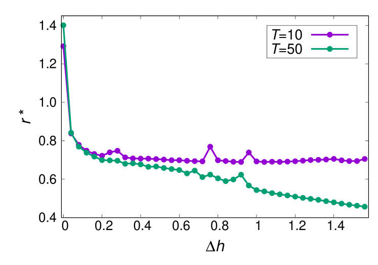
Figure 4: Normalized acceptance ratio $r^{*}$ (with the bin size 0.04) versus the field difference $\Delta h$ between two parent nodes for $h_{0}=0.8$ and $T=10,50$. The slow ($T=50$) and the fast ($T=10$) temporal changes of the external field exhibit very different behaviors, which can be compared with Fig. 3.

We next investigate the origin of the success of our proposed GA with focus put on the details of the mating stage. We measure the field difference $\Delta h\equiv|h^{a}(t)-h^{b}(t)|$ for parent systems $P_{a}$ and $P_{b}$ at $a$ and $b$, and compute the acceptance ratio $r$ of the offspring replacing the parent. For a better comparison, we use the normalized acceptance ratio $r^{*}\equiv r/r_{\rm avg}$ with $r_{\rm avg}$ being the time average of $r$ for $t\in[0,5000]$. Figure 4 shows $r^{*}$ versus $\Delta h$ for $T=10$ and 50 at $h_{0}=0.8$. We have chosen the two values $T=10$ and 50 to compare the difference between the fast and the slow temporal change (see Fig. 3). The region of relatively small values of $\Delta h$ in Fig. 4 mostly reflects what happens in the local mating, while larger values of $\Delta h$ are from the global mating.

In Fig. 4, $r^{*}$ for $T=50$ tends to decrease monotonically with $\Delta h$ while $r^{*}$ for $T=10$ appears to be insensitive to the change of $\Delta h$ in a broad region. Such a difference, we believe, indicates that a sufficiently large value of $T$ is required for the better performance of our method. In other words, only when the temporal change of the external field is sufficiently slow, our GA method becomes efficient to enjoy the benefit of the different environmental conditions across the whole system, yielding the better performance observed in Fig. 3. Consequently, we conclude that our GA exhibits an improved performance when the system has enough amount of spatial difference, which counteracts the innate tendency of homogenization in the conventional genetic algorithm.

4 Summary and Discussion

In this paper, we have proposed a genetic algorithm with the heterogeneous environmental condition, motivated by the effect of the geographic and temporal variation of environmental condition in natural evolution. Different environmental conditions can reduce intragroup diversity, but can enhance intergroup diversity.

We have used the three-dimensional spin-glass system as a genetic entity, and thus the lower-energy state of the system corresponds to the higher fitness in evolution. Our simulation results suggest that the existence of a certain degree of inhomogeneous and time-varying external field can help us to find a lower-energy state in a shorter computation time when the temporal period of the field is sufficiently large.

We again emphasize that in the present work we do not intend to propose the most efficient algorithm in finding the ground state of the spin-glass problem in particular. Even though our result in previous section only deals with a relatively higher energy regime $\approx$ -1.61 in comparison to the known ground state of target system $\approx$ -1.73[19], we use the spin-glass system only as an example to validate the general applicability of our method in a broad range optimization problems. In other words, we believe that our proposed genetic algorithm belongs to the meta-optimization methodology and thus can be applied in a broad research area. Original optimization problem can simply be extended to allow spatially and temporally varying environmental condition so that each local entity has a different but closely related fitness function. Genetic entities can then mate with each other, locally and remotely, which constitute the properly arranged heterogeneity in genetic system. For example, one can combine the environmental condition of our model with the crossover scheme of meiosis GA[7] or gendered GA[8], or the migration process of island model[13], with small modification of the objective function.

We argue that such wide applicability of our methodology ensures its potential practicality. Although the current framework of our GA is not appropriate to compare the performance with existing algorithms for a 3D spin-glass system, we expect that the central concept of our method is easily applicable to other existing methods to further enhance the performance. We conclude that different environmental conditions can be practically helpful in finding a better optimum in a shorter time, by allowing a certain level of genetic diversity in a gene pool. We plan to investigate other optimization problems by applying our suggested algorithm in the near future.

References

- [1] J. H. Holland, Adaptation in Natural and Artificial Systems, University of Michigan Press, Ann Arbor, MI, 1975, second edition, 1992.
- [2] D. E. Goldberg, Genetic Algorithms in Search, Optimization and Machine Learning, 1st Edition, Addison-Wesley Longman Publishing Co., Inc., USA, 1989.
- [3] R. Salomon, Gene1’1 c algorithms in optimal multistage distribution network planning, IEEE Trans. Power Syst. 9 (4) (1994) 1927 – 1933.
- [4] R. Salomon, Re-evaluating genetic algorithm performance under coordinate rotation of benchmark functions. a survey of some theoretical and practical aspects of genetic algorithms, Biosystems 39 (3) (1996) 263 – 278.
- [5] K. Gallagher, M. Sambridge, Genetic algorithms: A powerful tool for large-scale nonlinear optimization problems, Comput. Geosci. 20 (7) (1994) 1229 – 1236.
- [6] D. Gupta, S. Ghafir, An overview of methods maintaining diversity in genetic algorithms, Int. J. Emerging Technol. Adv. Eng. 2 (2012) 56–60.
- [7] N. Wiriyasermkul, V. Boobjing, P. Chanvarasuth, A meiosis genetic algorithm, in: 2010 Seventh International Conference on Information Technology: New Generations, 2010, pp. 285–289.
- [8] Sanchez-Velazco, J. Bullinaria, Gendered selection strategies in genetic algorithms for optimization, Artif. Intell. (10 2003).
- [9] M. Slatkin, Gene flow and the geographic structure of natural populations, Science 236 (4803) (1987) 787–792.
- [10] T. P. Craig, J. K. Itami, J. D. Horner, Geographic variation in the evolution and coevolution of a tritrophic interaction, Evolution 61 (5) (2007) 1137–1152.
- [11] J. N. Thompson, Specific hypotheses on the geographic mosaic of coevolution., Am. Nat. 153 (S5) (1999) S1–S14.
- [12] R. Tanese, J. H. Holland, Q. F. Stout, Distributed genetic algorithms for function optimization, Ph.D. thesis, USA, aAI9001722 (1989).
- [13] D. Whitley, S. Rana, R. Heckendorn, The island model genetic algorithm: On separability, population size and convergence, Journal of Computing and Information Technology 7 (12 1998).
- [14] S. F. Edwards, P. W. Anderson, Theory of spin glasses, J. Phys. Condens. Matter 5 (5) (1975) 965.
- [15] F. Barahona, On the computational complexity of ising spin glass models, J. Phys. A 15 (10) (1982) 3241.
- [16] S. Kirkpatrick, C. D. Gelatt, M. P. Vecchi, Optimization by simulated annealing, Science 220 (4598) (1983) 671–680.
- [17] J. Machta, Population annealing with weighted averages: A monte carlo method for rough free-energy landscapes, Phys. Rev. E 82 (2010) 026704.
- [18] A. A. Middleton, Improved extremal optimization for the ising spin glass, Phys. Rev. E 69 (2004) 055701.
- [19] K. F. Pál, The ground state energy of the edwards-anderson ising spin glass with a hybrid genetic algorithm, Physica A 223 (3) (1996) 283 – 292.
- [20] M. Palassini, F. Liers, M. Juenger, A. P. Young, Low-energy excitations in spin glasses from exact ground states, Phys. Rev. B 68 (2003) 064413.
- [21] K. F. Pál, Genetic algorithm with local optimization, Biol. Cybern. 73 (4) (1995) 335–341.