SuctionNet-1Billion: A Large-Scale Benchmark for Suction Grasping

Abstract

Suction is an important solution for the long-standing robotic grasping problem. Compared with other kinds of grasping, suction grasping is easier to represent and often more reliable in practice. Though preferred in many scenarios, it is not fully investigated and lacks sufficient training data and evaluation benchmarks. To address that, firstly, we propose a new physical model to analytically evaluate seal formation and wrench resistance of a suction grasping, which are two key aspects of grasp success. Secondly, a two-step methodology is adapted to generate annotations on a large-scale dataset collected in real-world cluttered scenarios. Thirdly, a standard online evaluation system is proposed to evaluate suction poses in continuous operation space, which can benchmark different algorithms fairly without the need of exhaustive labeling. Real-robot experiments are conducted to show that our annotations align well with real world. Meanwhile, we propose a method to predict numerous suction poses from an RGB-D image of a cluttered scene and demonstrate our superiority against several previous methods. Result analyses are further provided to help readers better understand the challenges in this area. Data and source code will be publicly available at www.graspnet.net.

I Introduction

Suction grasping is widely used in real-world pick-and-place tasks. Due to its simplicity and reliability, it is often preferred than parallel-jaw or multi-finger grasping in many industrial and daily scenes [1, 2, 3]. Though effective, it actually draws far less attention from researchers than the other types of grasping [4, 5, 6, 7, 8].

Recently, data-driven approach has made great progress in robotic grasping [4]. Since learning with real-robot is quite time-consuming, some researchers turned to build simulated environment to obtain large amount of synthetic data [6, 9]. However, learning from synthetic data faces the problem of visual domain gap, as analyzed in Section V-D1. Others tried to collect real-world data and annotate them manually [1]. However, the annotation process requires experience in robotic manipulation and is labor-intensive, especially for dense annotations, causing those datasets to be small in scale. Besides, although previous work [10] trained with with single-object scenes can transfer to cluttered scenes to some extent, later work [2] showed that training on cluttered scenes improved the model (see Section V-C1).

To further boost the development of suction grasping algorithms, a benchmark is needed to i) provide large-scale data with cluttered scenes captured by real-world sensors, ii) have dense annotations which is well aligned with real-robot trials, iii) evaluate suction poses quickly in a unified manner without access to a real robot. This is challenging due to the dilemma mentioned above: domain gap for synthetic data and difficulty to annotate real-world data manually. We address this issue by leveraging the advantage of both sides, which means we collect data using real-world sensors and annotate them by analytic computation with a physical model.

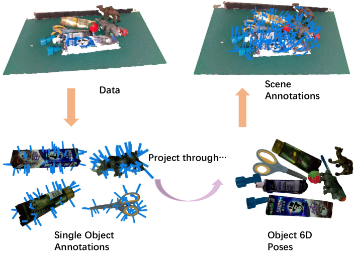
Figure 1: Our pipeline of building the dataset. For each single object, suction poses are sampled and annotated analytically with a physical model. Scene annotations are obtained by projecting the objects using their 6D poses. The pipeline enables generating large-scale dataset aligning well with real world without intensive human labor.

To obtain a large-scale densely annotated suction grasping dataset, we get inspiration from previous literature [4] and propose a two-step annotation pipeline. Specifically, we first generate and annotate suction poses on 88 single objects with their accurate 3D mesh models. Then we utilize objects’ 6D poses to generate dense annotations for totally 190 cluttered scenes by projection and collision detection. Each scene contains 512 RGB-D images captured by two cameras from 256 different views, leading to 97,280 images in total. Contributed to the effective annotation methodology, we built the first large-scale real-world suction grasping dataset in cluttered scenes with more than one billion suction annotations, which is larger than previous datasets by orders of magnitude. In addition, we provide an online evaluation system to quickly evaluate suction grasping algorithms in a unified manner. We conducted real-world experiments to show that our benchmark aligns well with real-robot manipulations. The pipeline of building our dataset is shown in Fig. 1. We hope the large-scale densely annotated real data as well as the evaluation metric can benefit related research.

With the new large-scale dataset, we propose a new method to predict 6D suction poses directly from single RGB-D image. Firstly, a neural network predicts a pixel-wise seal formation heatmap and a center map for objects from the RGB-D input. Then, we sample high-score suction candidates by grid sampling. Finally, we compute 3D suction points and directions from depth image geometrically with camera intrinsics. The effectiveness of our proposed method is demonstrated by experiments. Previous methods [10, 1] are also evaluated on our benchmark.

The rest of our paper is organized as follows: we firstly introduce previous methods and datasets in Sec. II. Next, in Sec. III, we detail the construction of our benchmark, including our analytical models, annotation procedure and evaluation metrics. Our network is then introduced in Sec. IV. Finally, abundant analyses to our benchmarks and several baseline methods are carried out in Sec. V.

II Related Work

In this section, we will review some previous suction-based grasping algorithms, previous suction-related datasets and suction analytic models.

II-A Suction Datasets

Zeng et al. [1] built a real-world dataset by seeking experts who had experience with suction grasp to annotate suctionable and non-suctionable areas on raw RGB-D images. However, the labor-intensive procedure and requirement of expertise makes it hard to build large-scale dataset. In the contrast, Mahler et al. [6, 10] turned to simulation and built a synthetic dataset by using 3D models and annotated suctions by analytical computing. The dataset contained depth images rendered from those 3D models. They built a much larger dataset but suffered from the problem of domain gap of visual perception and did not have RGB images.  [2] also pointed out that methods trained on single object scenes does not transfer well to cluttered scenes. Other datasets [11, 12] are either small in scale or publicly unavailable. In this work, we aim to provide a dataset that is both large in scale and aligns with real visual perception. An online evaluation system is further provided to enable algorithm evaluation without the need to access real robots

Meanwhile, our dataset contains 6D poses and thus can be used by researchers in 6D pose estimation community [13, 14, 15]. And these datasets can be used for suction purpose with our annotation pipeline.

II-B Suction Analytic Models

In the literature of graphics, Provot et al. [16] modeled deformable objects like cloth and rubber using a spring-mass system with several types springs. Mahler et al. [10] followed this work and modeled the suction cup as a quasi-static spring system. They evaluated whether the suction can form a seal against object surface by estimating the deformation energy. Readers can refer to a review by Ali et al. [17] for more constitutive models of rubber-like materials.

Assuming a seal is formed, several models have been designed to check force equilibrium. Most early works regarded the suction cup as rigid and considered forces along surface normals, tangential forces due to friction and pulling forces due to motion. Bahr et al. [18] and Morrison et al. [12] augmented the model by further considering moment resistance and torsional friction . Mahler et al. [10] combined both torsional friction and moment resistance. We follow the suction model in [10] due to its effectiveness and make some modifications to achieve fast and accurate annotations.

II-C Suction-based grasping

Eppner [19] firstly detected objects and then pushed objects from top or side until suction was achieved. Hernandez et al. [11] firstly recognized objects and estimated their 6D poses [20, 21]. They then generated suction candidates on the 3D model of the item based on primitive shapes. Those candidates were finally scored based on geometric and dynamic constraints. Zeng et al. [1] used a neural network trained on a human-labeled dataset to predict grasping affordance map from the RGB-D input and chose the suction point with max affordance value. Morrison et al. [12] firstly obtained semantic segmentation of the scenes and scored the suctions using heuristics like distance from boundary and object curvature. Mahler et al. [10] designed a network to score a suction candidate with the depth image centered at the suction point and suction pose information as input. Correa et al. [22] further proposed a toppling strategy to expose access to robust suction points and increase the suction reliability. Shao et al. [9] proposed an online self-supervised learning method by predicting suction and getting results from a simulated environment.

III SuctionNet-1Billion

In this section, we provide details of our benchmark and illustrate how we build it.

III-A Overview

Previous suction datasets are either small in scale [1] due to labor intensity and expertise required for annotators, or only contain synthetic data [10, 2] which can cause performance decrease in real world due to the domain gap. Also, DexNet3.0 [10] only focuses on single objects, which does not transfer well to cluttered scenes pointed out by [2]. To address those problems, we build a large-scale real-world dataset with cluttered scenes and dense suction pose annotations named SuctionNet-1Billion.

Our data is from GraspNet-1Billion [4], which contains 88 daily objects with high quality 3D mesh models and 190 cluttered scenes. Each scene contains 512 RGB-D images captured by two different cameras, RealSense and Kinect, from 256 views. Accurate object 6D pose annotations, object masks, bounding boxes and each view’s camera pose are also provided. For each image, we densely annotate suction poses by computing both seal formation scores and wrench resistance scores. Our dataset contains 3.3M $\sim$ 8.1M annotations for each scene and 1.1B in total.

III-B Suction Pose Annotation

We define a suction pose as a 3D suction point and a direction vector starting from the suction point and pointing outside of the object surface. Inspired by DexNet 3.0 [10], given a suction pose, we evaluate seal formation and wrench resistance separately. However, instead of labeling suction poses with binary scores, we assign them two continuous scores, namely seal score $S_{seal}$ and wrench score $S_{wrench}$, both in the range of $[0,1]$. We define the overall score as the product of these two scores $S=S_{seal}\times S_{wrench}$. In the following, we will describe how we compute the scores and present the overall annotation procedure.

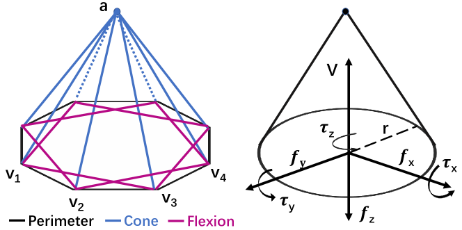
Figure 2: DexNet 3.0 [10] suction model. Left: the quasi-static spring model with three different springs represented by different colors. Right: Wrench basis for the suction cup. Best viewed in color.

III-B1 Seal Score Evaluation

DexNet 3.0 [10] models a suction cup as a quasi-static spring system with topology shown in Fig. 2 left. Specifically, the model has three kinds of springs: 1) Perimeter Springs – those linking vertex v_i to vertex v_i+1; 2) Cone Springs – those linking vertex v_i to vertex a, ; 3) Flexion Springs – those linking vertex v_i to vertex v_i+2.

They project the cup along the suction direction to the suction point on the object surface. The length of each spring will change due to the irregularity of the surface. If each spring’s length change is within $10\%$, seal formation is labeled as positive, otherwise negative.

We modify the annotation process as follows. Firstly, we remove Cone Springs and Flexion Springs and only keep Perimeter Springs since the three types of springs are coupled with each other. Secondly, we model the score as a continuous value instead of a binary one. Define $l_{i}$ as the length of the perimeter spring linking vertex v_i and vertex v_i+1. Given the original length $l_{i}$ and the length after projection $l^{\prime}_{i}$, we get the change ratio as:

$$r_{i}=min(1,\lvert\frac{l^{\prime}_{i}-l_{i}}{l_{i}}\rvert).$$ (1)

The spring deformation score is then defined as:

$$S_{deform}=1-max\{r_{1},r_{2},...,r_{n}\}.$$ (2)

Thirdly, to compensate for accuracy loss induced by representing a circle as polygon, we fit a plane for object surface points around the contact ring using least-squares solution and calculate the average of squared errors from the surface points to the plane, denoted as $E_{square}$. The plane fit score is defined as:

$$S_{fit}=e^{-c\cdot E_{square}}.$$ (3)

Where $c>0$ is some fixed coefficient. Finally, the seal score is defined as the product of $S_{deform}$ and $S_{fit}$:

$$S_{seal}=S_{deform}\times S_{fit}.$$ (4)

Note that we check if all the vertexes of suction gripper can be projected onto the object before the computation. If any vertex falls out of the object (e.g. suction center is near the object edge), $S_{seal}$ will be 0.

We conduct real-robot experiments in Sec. V-A to demonstrate that our annotations align well with real world suctions.

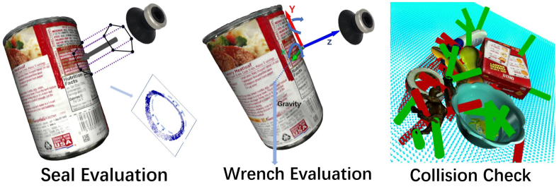
Figure 3: Our annotation Procedure. Left: For each object, Seal Formation Score $S_{seal}$ is annotated by projecting the suction cup to the object; then max deformation ratio of the springs and the average residual errors from the points around the contact ring and a fitted plane are computed to get the score. Middle: Wrench Score $S_{wrench}$ is computed after projecting the objects with their 6D poses in a scene considering the wrench caused by gravity around axis X and Y. Right: Scene collision is checked in each scene where red represents collision while green represents collision-free. Best viewed in color.

III-B2 Wrench Score Evaluation

To lift up an object, the suction end-effector should be able to resist the wrench caused by gravity. DexNet 3.0 [10] defined 5 kinds of basic wrenches, namely 1) Actuated Normal Force ($f_{z}$); 2) Vacuum Force ($V$); 3) Frictional Force ($f_{f}=(f_{x},f_{y})$); 4) Torsional Friction ($\tau_{z}$) and 5) Elastic Restoring Torque ($\tau_{e}=(\tau_{x},\tau_{y})$) as shown in Fig. 2 right. The following 3 constraints are defined:

$$\begin{split}Friction:&\sqrt{3}|f_{x}|\leq\mu f_{N}\quad\sqrt{3}|f_{y}|\leq\mu f_{N}\quad\sqrt{3}|\tau_{z}|\leq r\mu f_{N},\\ Material:&\sqrt{2}|\tau_{x}|\leq\pi rk\quad\sqrt{2}|\tau_{y}|\leq\pi rk,\\ Suction:&f_{z}\geq-V,\end{split}$$ (5)

where $\mu$ is the friction coefficient, $f_{N}=f_{z}+V$ is the normal force between the suction cup and object, $r$ is the radius of the contact ring and $k$ is a material-related constant modeling the maximum stress for which the suction cup has linear-elastic behavior. They label the wrench resistance as positive if all the constraints are satisfied otherwise negative.

We simplify the wrench score evaluation by removing the Friction and Suction constraints in Eq. 5. The reason we remove the Friction constraint is that it requires the suction cup to stick on the object surface while keeping the seal, which is usually satisfied in suction manipulations. As for the Suction constraint, it does not contribute to the suction policy because if $V$ is less than the object gravity, then all suctions will fail no matter where the suction point is. Therefore, we assume this constraint is always satisfied.

The wrench score is also modified to be continuous in $[0,1]$. Specifically, we define a torque threshold as $\tau_{thre}=\pi rk$ and overall tangential torque as $|\tau_{e}|=\sqrt{\tau_{x}^{2}+\tau_{y}^{2}}$. The wrench score is defined as:

$$S_{wrench}=1-min(1,|\tau_{e}|/\tau_{thre}).$$ (6)

Note that $|\tau_{e}|$ is actually related to the weight of object but we simply assign the same weight to each object. The weight actually does not contribute to the policy because given any weight $m$, the gravity wrench is $\tau=mgl$ where $g$ is the gravity acceleration constant. The policy should try to minimize the force arm $l$ which is dependent on the suction point and direction (i.e. suction pose) regardless of the weight. In other words, the optimal suction pose is actually the same for different weights.

TABLE I: Ground truth score distribution for different splits.

Range	Train			Test-Seen			Test-Similar			Test-Novel
	$S_{seal}$	$S_{wrench}$	$S$	$S_{seal}$	$S_{wrench}$	$S$	$S_{seal}$	$S_{wrench}$	$S$	$S_{seal}$	$S_{wrench}$	$S$
$[0.0,0.2)$	35.5%	24.8%	55.5%	35.3%	23.4%	53.0%	27.4%	18.2%	41.8%	72.4%	24.5%	82.8%
$[0.2,0.4)$	5.5%	11.7%	12.0%	5.5%	11.5%	12.2%	3.7%	13.6%	13.9%	4.5%	13.2%	7.0%
$[0.4,0.6)$	5.6%	22.6%	17.0%	5.5%	22.6%	17.2%	4.1%	26.5%	23.2%	4.2%	23.6%	6.1%
$[0.6,0.8)$	9.4%	26.9%	11.9%	9.4%	28.9%	13.7%	9.6%	28.5%	16.0%	4.7%	26.6%	3.3%
$[0.8,1.0]$	43.9%	13.9%	3.6%	44.4%	13.5%	3.8%	55.3%	13.3%	5.2%	14.2%	12.1%	0.8%

TABLE II: Summary of the properties of publicly available suction datasets. ”Obj.”, ”img.” and ”Modal.” are short for Objects, Images and Modality. ”Cam.” and ”Sim.” are short for Camera and Simulation. ”-” means unknown.

Data	Labels /scene	Obj. /scene	Total labels	Total img.	Modal.	Data	CAD
[10]	1	1	2.8M	2.8M	depth	sim.	Yes
[2]	1	1	2.5M	2.5M	depth	sim.	Yes
[1]	$\sim$100K	-	191M	1837	rgbd	1 cam.	No
[14]	None	$\sim$5	None	134K	rgbd	1 cam.	Yes
ours	$\sim$5.1M	$\sim$10	1.1B	97K	rgbd	2 cam.	Yes

III-B3 Overall Procedure

6D Pose Annotation

We adopt the 6D pose annotations from GraspNet-1Billion [4]. The annotations are obtained by propagating the annotated 6D poses of the first frame of each scene using the recorded camera poses:

$$\textbf{P}_{i}^{j}=\textbf{cam}_{i}^{-1}\textbf{cam}_{0}\textbf{P}_{0}^{j},$$ (7)

where $\textbf{P}_{i}^{j}$ is the 6D pose of object j at frame i and $\textbf{cam}_{i}$ is the camera pose of frame $i$. We refer readers to [4] for more details about object collection and 6d pose annotation.

Suction Pose Annotation

Following GraspNet-1Billion [4], we adopt the two-step pipeline to annotate suction poses: annotate single objects and then project to scenes.

Firstly, we sample and annotate suction poses on each single object. The 3D mesh models are first voxelized (voxel side length is 5 $mm$) and suction points with the corresponding directions (surface normals) are sampled uniformly in voxel space.

Secondly, for each scene, these suction poses are projected using the annotated 6D object poses:

$$\begin{split}&\textbf{P}^{i}=\textbf{cam}_{0}\textbf{P}^{i}_{0},\\ &\mathbb{S}^{i}_{(w)}=\textbf{P}^{i}\cdot\mathbb{S}^{i}_{(o)},\end{split}$$ (8)

where $\textbf{P}_{i}$ is the 6D pose of the $i$-th object in the world frame, $\mathbb{S}^{i}_{(o)}$ is a set of suction poses in the object frame and $\mathbb{S}^{i}_{(w)}$ contains the corresponding poses in the world frame.

The seal scores can be directly obtained from each single objects since they only depend on local surface geometry while the wrench scores should be annotated per-scene since the wrenches depend on object poses. We also check collision to avoid invalid suctions. Specifically, we model the suction end-effector as a cylinder and check if there are object points in it. After the above three steps, we get dense suction annotations for each scene. The key parts of annotation is illustrated in Fig. 3.

The ratios of each score interval for both Seal Score and Wrench Score are listed in Table I. Seal scores are mostly distributed in the ranges of $[0.0,0.2)$ and $[0.8,1.0]$ since it is usually quite clear whether it can form a seal or not while wrench scores are distributed more evenly since suction points are sampled uniformly from the 3D space.

III-C Evaluation Metrics

Dataset Split

We use the same split as [4]. Among all 190 scenes, there are 100 for training and 90 for testing. The testing set can be divided into 3 categories: 30 scenes with seen objects, 30 with unseen but similar objects and 30 for novel and adversarial objects. As we can see in Table I, the Test-Seen and Test-Similar set share similar distribution with the Train set. The Test Novel set is very hard, where only a small number of suctions get high scores.

Metrics

Given a suction pose, we first associate it with the target object by checking which object is closest to the suction point. Then the evaluation process is similar with annotation. After computing the seal score $S_{seal}$ and wrench score $S_{wrench}$ separately, the final score is obtained by production $S=S_{seal}\times S_{wrench}$.

Given a cluttered scene, suction pose prediction algorithms should predict multiple grasps. Following [4], we use Precision@k as our metrics, which measures the precision of top-k ranked suctions. Since the evaluation score is continuous instead of binary, we define several score thresholds to decide whether a suction is positive, that is, if the score of a suction is larger than a threshold $s$, then it is regarded as positive under threshold $s$. AP_s denotes the average of Precision@k under the threshold $s$, where k ranges from 1 to 50. Similar to previous works [4], AP_s under different threshold $s$ is reported. We also report the overall AP as the average of AP_s with $s$ ranging from 0.2 to 0.8, with an interval $\delta s=0.2$.

To prevent hacking on testset by predicting many similar suction poses and encourage diverse suction poses, we run Non-Maximal Suppression (NMS) [4] before evaluation and restrict the maximal number of suctions on a single object to 10.

Since we usually perform the best suction candidate given any scenes, we also report AP and AP_s of the top-1 suction pose (which only calculates Precision@1), denoted as AP-top1 and AP_s-top1.

III-D Summary

As mentioned before, real-world data and dense annotations contradict to each other to some extent but thanks to our annotation system and data collected by [4], we build a real-world dataset with much larger scale and diversity. Comparison with other publicly available suction dataset is shown in table II.

As for evaluation, continuity in suction space leads to infinite number of possible suction candidates. Therefore, no matter by human annotation [1] or simulation, it is unlikely to cover all possible suction predictions. To this end, following [4], we do not provide pre-computed labels for test set, but directly evaluate them by computing scores with our evaluation system. The API will be made publicly available.

A robot system can basically be separated into two parts: perception part and control part. Our benchmark falls into the first category, focusing on the problem of suction pose prediction from visual input and leaving out the control part. We make our annotations irrelevant to real robotic design choices as much as we can. Although the data comes from the previous work [4], due to the different topology and working mechanism of the end-effectors, the annotation algorithm is totally different. As mentioned in Sec. I, suction has several advantages compared with parallel-jaw grasping but lacks enough investigation, we hope our benchmark can help researchers design their suction prediction algorithms and compare with others fairly.

TABLE III: Real-robot success rates / average scores in different score ranges. ”-” means that there are not enough labeled suction candidates in the range.

Object ID	$S_{seal}\in[0,0.2]$	$S_{seal}\in[0.4,0.6]$	$S_{seal}\in[0.8,1.0]$	Object ID	$S_{seal}\in[0,0.2]$	$S_{seal}\in[0.4,0.6]$	$S_{seal}\in[0.8,1.0]$
000	8% / 0.045	48% / 0.505	100% / 0.980	031	0% / 0.000	- / -	100% / 0.863
005	4% / 0.008	60% / 0.538	92% / 0.881	036	0% / 0.029	40% / 0.477	100% / 0.977
010	12% / 0.075	56% / 0.524	100% / 0.964	046	4% / 0.001	44% / 0.492	100% / 0.950
015	9.1% / 0.068	52.9% / 0.495	100% / 0.945	063	8% / 0.039	56% / 0.509	92% / 0.910
024	4% / 0.026	48% / 0.513	96% / 0.950	065	4% / 0.024	48% / 0.523	96% / 0.929

IV Method

In this section, we will describe our end-to-end suction pose prediction framework. We will first introduce the problem formulation and then describe our framework pipeline.

IV-A Problem Formulation

To let a robot perform a suction grasping, we need to tell it where to place the suction cup and how it should approach the object. Therefore, we define a suction grasping pose as:

$$\textbf{S}=[\textbf{p},\textbf{u}],$$ (9)

where p is the suction point, a.k.a. the center of contact ring between suction cup and object and u is the direction vector pointing from the suction point outside the object surface.

We define the prediction task as, given a RGB-D image of a cluttered scene from a specific viewpoint, the algorithm should predict a set of reasonable suction poses $\mathbb{S}$. Based on that, our framework is formulated as follows.

IV-B Framework

We assume the camera intrinsics are known so we can project a 2d pixel coordinate to its 3D point. Our pipeline is illustrated in Figure 4, which is composed of 3 steps: 1) 2D heatmap prediction, which predicts pixel-wise suction scores; 2) sampling a fixed number of suction points; 3) suction direction estimation.

Figure 4: Our proposed pipeline. Given an RGB-D image, our network predicts a seal score heatmap and center score heatmap separately. The two heatmaps are then multiplied to get a final score map. We perform grid sampling on the final score and project the sampled pixels to 3D space. Suction directions are simply obtained by estimating the normals of corresponding points.

Heat Map Prediction

Instead of directly predicting the final suction scores, we decouple the heatmap into two separate heatmaps, namely seal heatmap and wrench heatmap, corresponding to seal score and wrench score mentioned in Sec. III-B. Similarly, the final heatmap is obtained by multiply the two heatmaps pixel-wise.

We adopt DeepLabv3+ [23] for heatmap prediction because they have key designs to deal with different object sizes and to better recognize object boundary. Specifically, we use ResNet-101 [24] as the encoder and modify the input channel of the first convolution layer from 3 to 4 (RGB to RGB-D).

Since suction poses are labeled in 3D space, to get the 2d label of seal score heatmap, we first project the 3D points onto 2D image using the camera intrinsics. To inpaint the empty pixels caused by voxel sampling, we draw a local Gaussian heatmap around each projected pixel. As for wrench heatmap label, inspired by CenterNet [25], we draw a center heatmap to approximate the wrench heatmap for efficiency. The network is trained with MSE (Mean Squared Error) loss function.

Downsampling Suctions

The goal of our framework is to predict a fixed number of suction poses for each scene. However, the predicted heatmap is too dense to directly recover suction poses from pixels. Therefore, we propose a simple but effective sampling strategy. Specifically, we first divide the image to several regular grids and sample the suction with the highest predicted score within each grid. We then rank these sampled suction proposals and output the pixel coordinates of the top 1024 suctions, which can be further converted to 3D points with the camera intrinsics.

Suction Direction Estimation

We simply use the surface normals of the suction points as direction. Specifically, we first create point cloud from the depth image and use Open3D [26] to directly estimate normals.

Figure 5: The qualitative results of our method. Scenes are constructed from RGB-D image using the camera intrinsics. Suctions are represented by blue cylinders.

TABLE IV: Evaluation for different methods. The table shows the results on data captured by Kinect/RealSense respectively.

Metric	Methods	Seen			Similar			Novel
		AP	AP0.8	AP0.4	AP	AP0.8	AP0.4	AP	AP0.8	AP0.4
Top-50	Normal STD	6.16/10.10	0.74/1.01	7.20/12.64	17.54/19.23	2.38/2.26	24.68/25.95	1.34/3.50	0.12/0.23	1.08/4.22
	DexNet3.0 [10]	9.46/15.50	0.96/1.53	11.90/20.22	14.93/18.92	2.45/2.62	19.05/24.51	1.68/2.62	0.04/0.35	1.89/5.32
	Zeng et al. [1]	14.82/28.31	1.00/3.37	20.02/38.58	14.23/26.15	1.61/3.35	18.66/34.83	2.85/7.79	0.17/0.38	3.35/9.78
	Ours	15.94/28.31	1.25/3.41	20.89/38.56	18.06/26.64	1.96/3.42	24.00/35.34	3.20/8.23	0.23/0.35	3.78/10.29
Top-1	Normal STD	11.68/15.40	1.94/1.82	13.35/18.83	34.11/31.20	6.51/4.74	47.28/43.46	2.64/4.89	0.28/0.52	3.72/5.96
	DexNet3.0 [10]	12.30/10.61	3.36/1.30	15.03/13.91	20.75/14.28	5.39/2.40	26.00/17.71	1.09/2.81	0.08/0.29	1.17/3.15
	Zeng et al. [1]	25.48/42.59	1.97/6.78	34.84/60.70	14.88/35.56	1.46/4.52	19.02/48.95	7.13/13.15	0.17/0.12	7.98/19.80
	Ours	26.44/43.98	2.90/7.79	35.98/60.81	24.59/36.59	2.45/6.54	32.89/49.30	6.66/14.32	0.13/0.38	8.80/19.95

V Experiments

In this section, we will first show that our ground-truth annotations align well with real-world suction through robotic experiments and then compare several representative methods with our method using the unified metrics introduced in Sec. III-C.

V-A Annotation Evaluation

We conduct real-robot experiments to show that our Seal Score annotations align well with the real world. The Wrench Score annotations are omitted because we make it a relative score to remove the dependence on specific object weights. We paste ArUco code on the objects to get their 6D poses in our experiment.

For the hardware setting, we use a common UR5 robotic arm with an Intel RealSense D435 RGB-D camera. 12 objects are picked from our dataset (shown in Fig. 6). To verify the consistency of our annotation and the real-world suction success rate, we choose the annotated suction poses from three representative score ranges: [0,0.2], [0.4,0.6], [0.8,1.0] and conduct real-world suction. For each score range, 25 suction poses are picked randomly. The suction success rates and the average annotation scores of executed suction poses are shown in Table III. As we can see, the success rates align well with the scores.

V-B Baseline Introduction

We evaluate three baseline methods listed below:

Normal STD

This method estimates the corresponding normal for each pixel and compute the standard deviation (STD) $\sigma$ within a local patch. The $\sigma$ is normalized to $[0,1]$ by dividing the maximal standard deviation value in the image. The final score for each pixel is computed as $S=1-\sigma$. A bounding box indicating the location of the objects is used as an additional input otherwise most predicted suction points will lie on the flat table.

Figure 6: objects we use to do real-robot evaluation.

DexNet 3.0

Mahler et al. [10] trained a network named GQCNN to predict a score given the suction pose and the depth image centered at the suction point. To get suction poses, they first uniformly sample initial suction poses, predict their scores and finally post process the suctions with Cross Entropy Method. We directly evaluate their pretrained model on our benchmark.

Fully Convolutional Network

Zeng et al. [1] propose to use a fully convolutional network to predict heatmap given a RGB-D image. Specifically, they use two branches of ResNet-101 [24] to learn from RGB image and depth image separately. The features from two branches are then fused to predict suction score. Finally, the predicted scores are upsampled bilinearly to original resolution. We use the same training data, loss function, downsampling and normal estimation steps as ours, mentioned in Sec. IV-B, to modify the network to our setting.

V-C Results and Analysis

The results are listed in Table IV. We provide some analysis below.

V-C1 Performances of Different Algorithms

As we can see, our method performs the best among all the methods even without additional object bounding box as input. DexNet 3.0 [10] performs worse than [1] and our method. There can be two reasons. The first one is due to domain gap as shown in Section V-D1. The second is that DexNet 3.0 was trained with single objects so it had difficulty transferring to multi-object scenes. The evidence of the difficulty can be found in Figure 3.C of DexNet 4.0 [2], the network trained with 100 objects and 2.5k heaps has a higher reliability compared with the one trained with 1.6k objects and 100 heaps, especially in level 2.

V-C2 Performances on Different Splits

As we can see, performances of different algorithms on the Test-Similar set is generally the highest. The reason is that this set contains objects easier to perform suction on, just as indicated in Table I. Though simpler, the set is still suitable to evaluate algorithms’ ability of generalization, which is indicated by the relative performance difference between the Normal STD method and our neural network. Since the Normal STD method does not have the problem of generalization, less advantage of our method indicates the need of generalization. The performances on the Test Novel set are all quite low. The reason is that the set contains new and adversarial objects with few proper suction points, as shown in Table I

V-C3 Top-1 performance

We can see from IV that our method also outperforms previous methods under the Top-1 metric. An exception is that our network fails to outperform the traditional Normal STD method on the Similar split with Kinect. The reason is that Kinect camera has a wide view so the objects look small in the images. with an additional bounding box indicating where the objects are, the traditional method does not face the problem. In practice, we can eliminate such problem by cropping the images.

V-D Ablation Study

V-D1 Domain Gap Analysis

We analyze the domain gap of both RGB images and depth images. To show the domain gap of RGB images, since our network is trained with real RGB-D images, we further test it on the synthetic RGB with real depth images and see how much the performance will decrease, which can give us the same insight with training on synthetic data and testing on real data. To show the domain gap of depth images, we compare the performance difference of DexNet 3.0 [10] since it only takes depth images as input.

Table V shows the results on the similar split. There do exist domain gaps with regard to the two different inputs, especially for RGB images. The results of depth images are relatively small but the gap will increase if we only compare the top 1 suction poses.

Examples of the depth images and RGB images can be found in Figure 7.

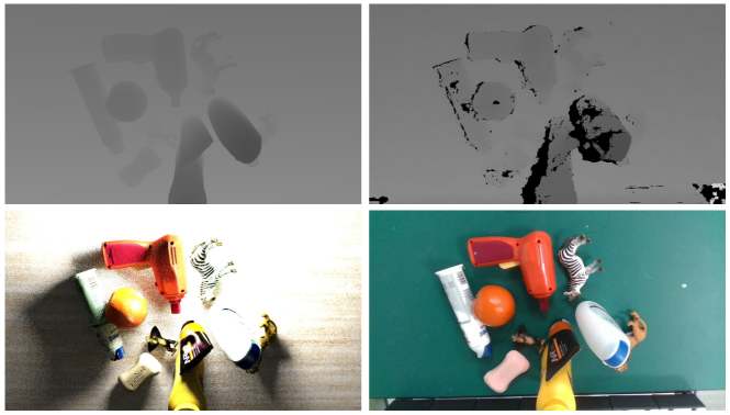
Figure 7: Examples of both synthetic (left column) and real (right column) depth images (top row) and RGB images (bottom row).

TABLE V: Ablation study of the domain gap

Network	Data	Num Suctions	AP	AP0.8	AP0.4
Ours	Synthetic RGB	Top 50	7.75	1.39	10.07
	Real RGB	Top 50	26.64	3.42	35.33
	Synthetic RGB	Top 1	3.33	0.00	0.00
	Real RGB	Top 1	36.59	6.54	49.30
DexNet 3.0 [10]	Synthetic depth	Top 50	20.61	2.64	26.36
	Real depth	Top 50	18.92	2.62	24.51
	Synthetic depth	Top 1	17.79	2.99	22.01
	Real depth	Top 1	14.28	2.40	17.71

V-D2 Different data scale

To show the necessity of the large data scale, we test the results of training with different data scale: $1/10$, $1/3$ and full dataset. The results can be found in Table VI. The performance increases significantly with the increase of data scale.

TABLE VI: Results trained with different dataset scales.

scale	AP	$AP_{0.8}$	$AP_{0.4}$
$1/10$	3.71	0.30	4.67
$1/3$	23.93	2.94	31.53
full	26.64	3.42	35.33

V-D3 Effect of RGB

In this section, we study the effect of RGB input. The results are shown in Table. VII. As we can see, model with extra RGB input perform much better on the seen split, especially for the top-1 predictions. Also, the results on the novel split indicates that RGB data can help make better predictions on hard objects. For the similar set, the model with only depth input performs better on realsense camera. We suppose that’s because depth has better generalization ability compared with RGB, just as shown in Table V.

TABLE VII: Ablation study of RGB Input on kinect/realsense camera.

Num Suctions	Input	Seen	Similar	Novel
Top 50	RGB-D	15.29/28.32	18.06/26.64	3.33/8.23
	Only Depth	13.84/22.89	17.57/28.83	3.23/7.31
Top 1	RGB-D	26.44/43.98	24.59/36.59	6.66/14.32
	Only Depth	19.52/30.54	18.26/39.39	4.69/10.47

V-E Real-robot Experiments

To show the effectiveness of our overall system, we deploy our network and DexNet 3.0 [10] separately on a UR5 robot arm and compare their performances. To get a comprensive comparison, we adopt three different metrics. The first is the ratio of the number of successful grasps to the number total grasps, denoted as $R_{grasp}$; the second is the ratio of the number of successfully cleared objects to the number of total objects, denoted as $R_{object}$; the last one is the ratio of the number of successfully cleared objects to the number of total grasps on those objects (the number of total grasps minus the grasps on the failed objects), denoted as $R_{mixture}$. We judge if the experiment terminates by observing if the robot fails to grasp any object in consecutive 3 times. As shown in Table VIII, our network outperforms DexNet3.0 [10] in terms of all the three metrics.

TABLE VIII: Performance comparison between DexNet3.0 [10] and our network in terms of three different metrics described in the above paragraph.

Metrics	DexNet 3.0 [10]	Ours
$R_{grasp}$	$16/28=57.14\%$	$25/31=80.65\%$
$R_{object}$	$16/20=80\%$	$25/25=100\%$
$R_{mixture}$	$16/21=76.19\%$	$25/31=80.65\%$

VI Conclusion

In this paper, we provide a large-scale dataset annotated on real-world data of cluttered scenes. To get grid of the need of intensive human labor and expertise, we design a physical model to analytically annotate large numbers of suction poses and adapt a two-step methodology to generate scene annotations from single object annotations. The accuracy of analytical annotations is proved by real-robot experiments. An unified evaluation system is further provided for fair comparison between algorithms. Meanwhile, we propose a pipeline to predict suction poses from an RGB-D image and provide detailed analysis. We hope our work can benefit related research.

References

- [1] A. Zeng, S. Song, K.-T. Yu, E. Donlon, F. R. Hogan, M. Bauza, D. Ma, O. Taylor, M. Liu, E. Romo et al., “Robotic pick-and-place of novel objects in clutter with multi-affordance grasping and cross-domain image matching,” in 2018 IEEE international conference on robotics and automation (ICRA). IEEE, 2018, pp. 1–8.
- [2] J. Mahler, M. Matl, V. Satish, M. Danielczuk, B. DeRose, S. McKinley, and K. Goldberg, “Learning ambidextrous robot grasping policies,” Science Robotics, vol. 4, no. 26, p. eaau4984, 2019.
- [3] M. Schwarz, C. Lenz, G. M. García, S. Koo, A. S. Periyasamy, M. Schreiber, and S. Behnke, “Fast object learning and dual-arm coordination for cluttered stowing, picking, and packing,” in 2018 IEEE International Conference on Robotics and Automation (ICRA). IEEE, 2018, pp. 3347–3354.
- [4] H.-S. Fang, C. Wang, M. Gou, and C. Lu, “Graspnet-1billion: A large-scale benchmark for general object grasping,” in Proceedings of the IEEE/CVF Conference on Computer Vision and Pattern Recognition, 2020, pp. 11 444–11 453.
- [5] M. Gou, H. Fang, Z. Zhu, S. Xu, C. Wang, and C. Lu, “Rgb matters: Learning 7-dof grasp poses on monocular rgbd images,” International Conference on Robotics and Automation (ICRA), pp. 1–8, 2021.
- [6] J. Mahler, J. Liang, S. Niyaz, M. Laskey, R. Doan, X. Liu, J. A. Ojea, and K. Goldberg, “Dex-net 2.0: Deep learning to plan robust grasps with synthetic point clouds and analytic grasp metrics,” Robotics: Science and Systems (RSS), pp. 1–8, 2017.
- [7] A. ten Pas, M. Gualtieri, K. Saenko, and R. Platt, “Grasp pose detection in point clouds,” The International Journal of Robotics Research, vol. 36, no. 13-14, pp. 1455–1473, 2017.
- [8] H. Liang, X. Ma, S. Li, M. Görner, S. Tang, B. Fang, F. Sun, and J. Zhang, “Pointnetgpd: Detecting grasp configurations from point sets,” in 2019 International Conference on Robotics and Automation (ICRA). IEEE, 2019, pp. 3629–3635.
- [9] Q. Shao, J. Hu, W. Wang, Y. Fang, W. Liu, J. Qi, and J. Ma, “Suction grasp region prediction using self-supervised learning for object picking in dense clutter,” in 2019 IEEE 5th International Conference on Mechatronics System and Robots (ICMSR). IEEE, 2019, pp. 7–12.
- [10] J. Mahler, M. Matl, X. Liu, A. Li, D. Gealy, and K. Goldberg, “Dex-net 3.0: Computing robust vacuum suction grasp targets in point clouds using a new analytic model and deep learning,” in 2018 IEEE International Conference on Robotics and Automation (ICRA). IEEE, 2018, pp. 1–8.
- [11] C. Hernandez, M. Bharatheesha, W. Ko, H. Gaiser, J. Tan, K. van Deurzen, M. de Vries, B. Van Mil, J. van Egmond, R. Burger et al., “Team delft’s robot winner of the amazon picking challenge 2016,” in Robot World Cup. Springer, 2016, pp. 613–624.
- [12] D. Morrison, A. W. Tow, M. Mctaggart, R. Smith, N. Kelly-Boxall, S. Wade-Mccue, J. Erskine, R. Grinover, A. Gurman, T. Hunn et al., “Cartman: The low-cost cartesian manipulator that won the amazon robotics challenge,” in 2018 IEEE International Conference on Robotics and Automation (ICRA). IEEE, 2018, pp. 7757–7764.
- [13] K. Kleeberger, C. Landgraf, and M. F. Huber, “Large-scale 6d object pose estimation dataset for industrial bin-picking,” in 2019 IEEE/RSJ International Conference on Intelligent Robots and Systems (IROS). IEEE, 2019, pp. 2573–2578.
- [14] Y. Xiang, T. Schmidt, V. Narayanan, and D. Fox, “Posecnn: A convolutional neural network for 6d object pose estimation in cluttered scenes,” Robotics: Science and Systems (RSS), pp. 1–8, 2018.
- [15] C. Rennie, R. Shome, K. E. Bekris, and A. F. De Souza, “A dataset for improved rgbd-based object detection and pose estimation for warehouse pick-and-place,” IEEE Robotics and Automation Letters, vol. 1, no. 2, pp. 1179–1185, 2016.
- [16] X. Provot et al., “Deformation constraints in a mass-spring model to describe rigid cloth behaviour,” in Graphics interface. Canada: Canadian Information Processing Society, 1995, pp. 147–147.
- [17] A. Ali, M. Hosseini, and B. Sahari, “A review of constitutive models for rubber-like materials,” American Journal of Engineering and Applied Sciences, vol. 3, no. 1, pp. 232–239, 2010.
- [18] B. Bahr, Y. Li, and M. Najafi, “Design and suction cup analysis of a wall climbing robot,” Computers & electrical engineering, vol. 22, no. 3, pp. 193–209, 1996.
- [19] C. Eppner, S. Höfer, R. Jonschkowski, R. Martín-Martín, A. Sieverling, V. Wall, and O. Brock, “Lessons from the amazon picking challenge: Four aspects of building robotic systems.” in Robotics: science and systems, 2016, p. 4831–4835.
- [20] Y. He, W. Sun, H. Huang, J. Liu, H. Fan, and J. Sun, “Pvn3d: A deep point-wise 3d keypoints voting network for 6dof pose estimation,” in Proceedings of the IEEE/CVF conference on computer vision and pattern recognition, 2020, pp. 11 632–11 641.
- [21] Z. Zhao, G. Peng, H. Wang, H.-S. Fang, C. Li, and C. Lu, “Estimating 6d pose from localizing designated surface keypoints,” arXiv preprint arXiv:1812.01387, 2018.
- [22] C. Correa, J. Mahler, M. Danielczuk, and K. Goldberg, “Robust toppling for vacuum suction grasping,” in 2019 IEEE 15th International Conference on Automation Science and Engineering (CASE). IEEE, 2019, pp. 1421–1428.
- [23] L.-C. Chen, Y. Zhu, G. Papandreou, F. Schroff, and H. Adam, “Encoder-decoder with atrous separable convolution for semantic image segmentation,” in Proceedings of the European conference on computer vision (ECCV), 2018, pp. 801–818.
- [24] K. He, X. Zhang, S. Ren, and J. Sun, “Deep residual learning for image recognition,” in Proceedings of the IEEE conference on computer vision and pattern recognition, 2016, pp. 770–778.
- [25] X. Zhou, D. Wang, and P. Krähenbühl, “Objects as points,” arXiv preprint arXiv:1904.07850, 2019.
- [26] Q.-Y. Zhou, J. Park, and V. Koltun, “Open3D: A modern library for 3D data processing,” arXiv:1801.09847, 2018.