Stochastic Reweighted Gradient Descent

Supplementary material

Abstract

Despite the strong theoretical guarantees that variance-reduced finite-sum optimization algorithms enjoy, their applicability remains limited to cases where the memory overhead they introduce (SAG/SAGA), or the periodic full gradient computation they require (SVRG/SARAH) are manageable. A promising approach to achieving variance reduction while avoiding these drawbacks is the use of importance sampling instead of control variates. While many such methods have been proposed in the literature, directly proving that they improve the convergence of the resulting optimization algorithm has remained elusive. In this work, we propose an importance-sampling-based algorithm we call SRG (stochastic reweighted gradient). We analyze the convergence of SRG in the strongly-convex case and show that, while it does not recover the linear rate of control variates methods, it provably outperforms SGD. We pay particular attention to the time and memory overhead of our proposed method, and design a specialized red-black tree allowing its efficient implementation. Finally, we present empirical results to support our findings.

1 Introduction

We are interested in the unconstrained minimization problem:

$$\min_{x\in\mathbb{R}^{d}}F(x)\coloneqq\mathop{\mathbb{E}}_{\xi\sim P}\left[f(x,\xi)\right]$$ (1)

where $\xi$ is a real random vector with distribution $P$. In machine learning, $x$ represents the parameters of the prediction rule, $\xi$ represents the pair of input/output variables, $f$ the loss function, and $F$ the risk.

In particular, we focus on the sample average approximation to (1):

$$\min_{x\in\mathbb{R}^{d}}F_{n}(x)\coloneqq\frac{1}{n}\sum_{i=1}^{n}f(x,\xi_{i})$$ (2)

where $(\xi_{i})_{i=1}^{n}$ are i.i.d. samples from $P$. This is also known as empirical risk minimization in machine learning.

Defining $f_{i}(x)\coloneqq f(x,\xi_{i})$ for $i\in[n]$, and letting $i$ be a uniformly distributed random variable on $[n]$, we can rewrite (2) as:

$$\min_{x\in\mathbb{R}^{d}}F(x)\coloneqq\frac{1}{n}\sum_{i=1}^{n}f_{i}(x)=\mathbb{E}\left[f_{i}(x)\right]$$ (3)

where the expectation is taken with respect to $i$.

We make the following assumptions on the function $F$ and the component functions $f_{i}$:

Assumption 1.

The function $F:\mathbb{R}^{d}\to\mathbb{R}$ is differentiable and $\mu$-strongly convex, that is $\forall x,y\in\mathbb{R}^{d}$:

$$F(y)\geq F(x)+\langle\nabla F(x),y-x\rangle+\frac{\mu}{2}\left\lVert y-x\right\rVert_{2}^{2}$$

Assumption 2.

For all $i\in[n]$, the functions $f_{i}:\mathbb{R}^{d}\to\mathbb{R}$ are differentiable and convex, that is, $\forall x,y\in\mathbb{R}^{d}$:

$$f_{i}(y)\geq f_{i}(x)+\langle\nabla f_{i}(x),y-x\rangle$$

Assumption 3.

For all $i\in[n]$, the functions $f_{i}:\mathbb{R}^{d}\to\mathbb{R}$ are $L$-smooth, that is, $\forall x,y\in\mathbb{R}^{d}$:

$$\left\lVert\nabla f_{i}(y)-\nabla f_{i}(x)\right\rVert_{2}\leq L\left\lVert y-x\right\rVert_{2}$$

Note that by Assumption 3 and the triangle inequality, $F$ is also $L$-smooth, and we define its condition number by $\kappa=L/\mu$.

Let $x^{*}$ be the unique minimizer of $F$. Our goal is to design the fastest algorithm that outputs a point $x\in\mathbb{R}^{d}$ such that $\left\lVert x-x^{*}\right\rVert_{2}^{2}<\varepsilon$ for a given accuracy $\varepsilon>0$. Following (Agarwal & Bottou, 2015), we assume that we have access to a gradient oracle that takes as input a point $x\in\mathbb{R}^{d}$ and an index $i\in[n]$ and returns $\nabla f_{i}(x)$. We then measure the complexity of an algorithm by counting the number of oracle calls needed to achieve a desired accuracy.

The most straightforward way to solve (3) is to ignore the particular structure of $F$, and simply run gradient descent or accelerated gradient-descent (Nesterov, 1983) on $F$. Under our assumptions and definition of complexity, gradient descent converges at the rate of $O(n\kappa\log{(1/\varepsilon)})$, while accelerated gradient descent converges at the rate of $O(n\sqrt{\kappa}\log{(1/\varepsilon)})$ (Nesterov, 2018). When $n$ is large, this becomes prohibitively expensive.

One solution to this is to view problem (3) in its expectation form, and use the stochastic approximation of gradient descent. This yields stochastic gradient descent (SGD) which estimates $\nabla F(x)$ by $\nabla f_{i}(x)$ for $i$ uniformly distributed on $[n]$ in the gradient descent update (Robbins & Monro, 1951; Nemirovsky & Yudin, 1983; Nemirovski et al., 2009; Moulines & Bach, 2011). The complexity of SGD under our assumptions is known to have two regimes. Denote by $\sigma^{2}$ the variance of the gradient estimator of SGD at the minimizer $x^{*}$. For $\varepsilon>\sigma^{2}/L\mu$, SGD converges at the fast rate $O(\kappa\log{(1/\varepsilon)})$, while for $\varepsilon\leq\sigma^{2}/L\mu$, SGD suffers from the sublinear rate $O(\sigma^{2}/\mu^{2}\varepsilon)$ (Needell et al., 2014; Nguyen et al., 2018; Gower et al., 2019). When $\sigma^{2}$ is large, SGD takes a long time to converge to even moderately accurate solutions.

While SGD does take into account the expectation form of the objective (3), it fails to adapt to the fact that the expectation is taken over a discrete distribution which gives rise to a finite-sum structure. The last decade has seen the development of many new methods that leverage this additional structure, including (but not limited to) SAG (Roux et al., 2012; Schmidt et al., 2017), SAGA (Defazio et al., 2014), SVRG (Johnson & Zhang, 2013), and SARAH (Nguyen et al., 2017). All of these methods converge at the fast linear rate of $O((n+\kappa)\log{(1/\varepsilon)})$. Further work in this direction led to the development of lower-bounds for the optimization of finite-sum functions under our assumptions and the oracle model of complexity (Agarwal & Bottou, 2015; Woodworth & Srebro, 2016; Arjevani, 2017; Lan & Zhou, 2018), and, similar to the deterministic case, accelerated methods have been developed that closely match them (Lin et al., 2018; Allen-Zhu, 2018; Lan et al., 2019; Song et al., 2020). The core innovation behind this set of algorithms is the design of more efficient gradient estimators using carefully designed control variates, earning them the name of variance-reduced methods.

Despite all this progress, SGD remains the algorithm of choice in practice for some machine learning problems where it empirically outperforms variance-reduced methods (Defazio & Bottou, 2019). From an optimization perspective, there are a few explanations to this observation.

One is the phenomenon of interpolation (Ma et al., 2018; Vaswani et al., 2019a, b): if $\sigma^{2}=0$, then SGD converges linearly for any $\varepsilon>0$ without any variance reduction. A second possible explanation is that in many cases we are content with a low accuracy solution $\varepsilon>\sigma^{2}/L\mu$, in which case SGD converges linearly as well. In either of these scenarios, SGD and variance-reduced methods have the same iteration complexity, but variance-reduced methods require on average three times as many gradient evaluations per iteration (SVRG/SARAH).

While these reasons can be used to explain the superior performance of SGD in some settings, there is evidence that there are scenarios where variance-reduction might be useful even when only moderate accuracy is needed. In particular, (Goyal et al., 2018) showed that reducing the variance of the gradient estimator by increasing the batch size leads to optimization gains in the training of deep neural networks for ImageNet. Even in such cases however, the user is faced with a new problem. If we use variance-reduced methods from the beginning of the optimization, we make progress three times more slowly than SGD in the initial phase, which is often the dominating phase. Ideally, we would like to pay the additional computational cost for variance-reduction only when we need it, but it is not clear how we can detect when progress becomes constrained by the variance of the gradient estimator, although some advances have been made in this direction, see for example (Pesme et al., 2020).

A pressing question that arises from our discussion is therefore: Can we develop a variance-reduced algorithm that uses exactly the same number of gradient evaluations as SGD ? Such an algorithm would enjoy the fast rate of SGD in the initial phase of optimization, while automatically performing variance-reduction when needed. This question is the main motivation for this paper.

Before closing this section, we give one additional motivation for our work. As previously mentioned, the core idea of variance-reduced methods is the use of carefully crafted control variates to reduce the variance of the gradient estimator. There are, however, other ways to reduce the variance of a Monte Carlo estimator. In particular, one can use importance sampling. There is a large literature on such methods. Initial attempts focused on using a fixed distribution throughout the optimization based on prior knowledge about the functions $f_{i}$ (Needell et al., 2014; Zhao & Zhang, 2015; Csiba & Richtárik, 2018), and were able to show slightly favorable rates compared to uniform sampling. A more recent line of work attempts to adaptively design the distributions (Schaul et al., 2015; Loshchilov & Hutter, 2015; Alain et al., 2016; Bouchard et al., 2016; Canevet et al., 2016; Stich et al., 2017; Katharopoulos & Fleuret, 2018; Johnson & Guestrin, 2018), although the methods developed in these works mostly rely on heuristics and do not come with theoretical guarantees. Finally, in an attempt to put adaptive importance sampling methods on a firmer theoretical ground, a recent set of papers embed the problem of designing the distributions in an online learning framework and propose methods that achieve sublinear regret (Namkoong et al., 2017; Salehi et al., 2017; Borsos et al., 2018, 2019; El Hanchi & Stephens, 2020). These analyses however are still not satisfactory as they assume that the gradient norms of the functions $f_{i}$ are uniformly bounded on $\mathbb{R}^{d}$ which does not hold, for example, when $F$ is strongly-convex. The second question we ask here is therefore: Can we develop a variance-reduced algorithm based on importance sampling and which provably outperforms SGD ?

Contributions: In this paper, we give positive answers to both questions. In particular, our contributions are as follows:

• We propose stochastic reweighted gradient descent (SRG), a variance-reduced algorithm for the optimization of finite-sums based on importance sampling.

• As oppose to SAGA/SAG which require $O(nd)$ memory, SRG only requires $O(n)$ memory.

• Unlike SVRG/SARAH which require on average three gradient evaluations per iteration, and like SGD, SRG requires a single gradient evaluation per iteration.

• We develop a specialized red-black tree that allows an efficient implementation of SRG, incurring an overhead of only $O(\log{n})$ operations per iteration compared to SGD.

• We show that SRG provably outperform SGD under our assumptions. Let $\sigma^{2}_{*}$ be the minimal variance achievable through importance sampling at the minimizer $x^{*}$. Then we show that SRG has the same convergence as SGD, but with $\sigma^{2}$ replaced with $\sigma_{*}^{2}$, which can be up to $n$ times smaller.

2 Algorithm

Algorithm 1 SRG

  Parameters: step sizes $(\alpha_{k})_{k=0}^{\infty}>0$, lower bounds $(\varepsilon_{k})_{k=0}^{\infty}\in(0,\frac{1}{n}]$

  Initialization: $x_{0}\in\mathbb{R}^{d},(g_{0}^{i})_{i=1}^{n}\in\mathbb{R}^{d}$

  for $k=0,1,2,\dotsc$ do

     $p_{k}=\operatorname*{arg\,min}_{p\in\Delta(\varepsilon_{k})}\frac{1}{n^{2}}\sum_{i=1}^{n}\frac{1}{p^{i}}\left\lVert g_{k}^{i}\right\rVert_{2}^{2}$

     sample $i_{k}\sim p_{k}$

     $x_{k+1}=x_{k}-\alpha_{k}\frac{1}{np_{k}^{i_{k}}}\nabla f_{i_{k}}(x_{k})$

     sample $b_{k}\sim\text{Bernoulli}(\frac{\varepsilon_{k}}{p_{k}^{i_{k}}})$

     $g_{k+1}^{i}=\begin{cases}\nabla f_{i}(x_{k})&\text{if}\ i=i_{k}\ \text{and}\ b_{k}=1\\ g_{k}^{i}&\text{otherwise}\\ \end{cases}$

  end for

Before introducing our proposed algorithm, let us first introduce some notation. For an iteration number $k\in\mathbb{N}$, SGD performs the following update to minimize (3):

$$x_{k+1}=x_{k}-\alpha_{k}\nabla f_{i_{k}}(x_{k})$$

for a step size $\alpha_{k}>0$ and a random index $i_{k}$ drawn uniformly from $[n]$ and independently at each iteration. The idea behind importance sampling is to instead sample the index $i_{k}$ according to a given distribution $p_{k}$ on $[n]$, and to perform the update:

$$x_{k+1}=x_{k}-\alpha_{k}\frac{1}{np_{k}^{i_{k}}}\nabla f_{i_{k}}(x_{k})$$

where $p_{k}^{i}$ is the $i^{th}$ component of the vector $p_{k}\in\Delta$, and $\Delta$ is the probability simplex in $\mathbb{R}^{n}$. It is immediate to verify that the importance sampling estimator of the gradient is unbiased as long as $p_{k}>0$. The challenge is to design a sequence $\{p_{k}\}_{k=0}^{\infty}$ that produces more efficient gradient estimators than the ones produced by uniform sampling.

Our proposed method is a simple modification of the one given by (El Hanchi & Stephens, 2020), and is given in Algorithm 1. The algorithm follows from the following reasoning. The variance of the importance sampling gradient estimator is given by, up to an additive constant:

$$\begin{split}\sigma^{2}(x_{k},p_{k})&\coloneqq\mathop{\mathbb{E}}_{i_{k}\sim p_{k}}\left[\left\lVert\frac{1}{np_{k}^{i_{k}}}\nabla f_{i}(x_{k})\right\rVert_{2}^{2}\right]\\ &=\frac{1}{n^{2}}\sum_{i=1}^{n}\frac{1}{p_{k}^{i}}\left\lVert\nabla f_{i}(x_{k})\right\rVert_{2}^{2}\end{split}$$ (4)

Ideally we would like to choose $p_{k}\in\Delta$ so that this variance is minimized, but this is not feasible as we do not have access to the gradient norms $\left\lVert\nabla f_{i}(x_{k})\right\rVert_{2}$. Inspired by control variates methods, and in particular SAG/SAGA, we instead maintain a table $(g_{k}^{i})_{i=1}^{n}$ that aims to track the component gradients $(\nabla f_{i}(x_{k}))_{i=1}^{n}$. We then use this table to construct an approximation of the true variance:

$$\tilde{\sigma}^{2}(x_{k},p_{k})\coloneqq\frac{1}{n^{2}}\sum_{i=1}^{n}\frac{1}{p^{i}_{k}}\left\lVert g_{k}^{i}\right\rVert_{2}^{2}$$ (5)

Finally, we choose $p_{k}$ so as to minimize this quantity. Since this is only an approximation, we perform the minimization over the restricted simplex $\Delta(\varepsilon_{k})=\{p\in\Delta\mid p\geq\varepsilon_{k}\}$ for a given $\varepsilon_{k}\in(0,1/n]$. This enforces $p_{k}>0$, while making sure the error on the approximation of the variance is taken into account. The difference between our method and the one proposed in (El Hanchi & Stephens, 2020) is in the way the table $(g_{k}^{i})_{i=1}^{n}$ is updated: we add a bernoulli random variable to determine whether the update occurs or not. This step is crucial for the analysis as we will see, although in practice it might be skipped.

The goal of the next two sections will be to (i) show that SRG can be efficiently implemented. (ii) analyse the convergence of SRG and show that it outperforms SGD.

3 Implementation

In this section, we show how Algorithm 1 can be efficiently implemented, leading to a per-iteration cost that is competitive with SGD.

First, note that while we use the table $(g_{k}^{i})_{i=1}^{n}$ in the presentation of Algorithm 1, in practice it is enough to store the gradient norms $(\left\lVert g_{k}^{i}\right\rVert_{2})_{i=1}^{n}$ only. SRG therefore requires only $O(n)$ memory compared to SAG/SAGA which require $O(nd)$ memory in general.

With memory issues out of the way, we turn to the main bottleneck in SRG which is sampling from:

$$p_{k}=\operatorname*{arg\,min}_{p\in\Delta(\varepsilon_{k})}\frac{1}{n^{2}}\sum_{i=1}^{n}\frac{1}{p^{i}}\left\lVert g_{k}^{i}\right\rVert_{2}^{2}$$ (6)

The following lemma, taken from (El Hanchi & Stephens, 2020), sheds some light on the solution:

Lemma 1.

Let $\{a_{i}\}_{i=1}^{n}$ be a non-negative set of numbers and assume that there is some $i\in[n]$ such that $a_{i}>0$. Let $\varepsilon\in[0,1/n]$, and let $\pi:[n]\rightarrow[n]$ be a permutation that orders $\{a_{i}\}_{i=1}^{N}$ in a decreasing order ($a_{\pi(1)}\geq a_{\pi(2)}\geq\dots\geq a_{\pi(N)}$). Define for $i\in[n]$:

$$\lambda(i)\coloneqq\frac{\sum_{j=1}^{i}a_{\pi(j)}}{1-(n-i)\varepsilon}$$ (7)

and:

$$\rho:=\max\left\{i\in[n]\;|\;a_{\pi(i)}\geq\varepsilon\lambda(i)\right\}$$ (8)

Then a solution of the optimization problem:

$$p^{*}=\operatorname*{arg\,min}_{p\in\Delta(\varepsilon)}\sum_{i=1}^{n}\frac{1}{p_{i}}a_{i}^{2}$$ (9)

is given by:

$$p^{*}_{i}=\begin{cases}a_{i}/\lambda(\rho)&\text{if $\pi(i)\leq\rho$}\\ \varepsilon&\text{otherwise}\end{cases}$$ (10)

In the case $a_{i}=0$ for all $i\in[n]$, any $p\in\Delta(\varepsilon)$ is a solution, and in the case $\varepsilon=1/n$, $p=1/n$ is the unique solution.

3.1 Naive implementation

Algorithm 2 Naive sample

  Input: $(a_{\pi(i)})_{i=1}^{n}>0,(\lambda(i))_{i=1}^{n},\varepsilon>0$

  Initialization: $l\leftarrow 1,r\leftarrow n$

  while $l\leq r$ do

     $m\leftarrow\lfloor\frac{l+r}{2}\rfloor$

     if $a_{\pi(m)}\geq\varepsilon\lambda(m)$ then

        $c\leftarrow m$

        $l\leftarrow m+1$

     else

        $r\leftarrow m-1$

     end if

  end while

  $\rho\leftarrow c$

  compute $p^{*}$ using (10).

  sample $i\sim p^{*}$.

  Output: the index $i$ and its probability $p^{*,i}$.

To simplify notation for this section we will use the one introduced in Lemma 1, that is, we will refer to $a_{i}$ instead of $\left\lVert g_{k}^{i}\right\rVert_{2}$.

Let us for the moment assume that we have access to $(a_{\pi(i)})_{i=1}^{n}$, a sorted version of $(a_{i})_{i=1}^{n}$, as well as to $(\lambda(i))_{i=1}^{n}$. We will worry about how to maintain these in the next subsection. How can we sample from (9) ?

The following proposition reveals a useful property, which we use to construct Algorithm 2:

Proposition 1.

With the definitions in Lemma 1, we have:

$$a_{\pi(i)}\geq\varepsilon\lambda(i) \Rightarrow a_{\pi(l)}\geq\varepsilon\lambda(l)\quad\forall l\leq i$$

$$a_{\pi(i)}<\varepsilon\lambda(i) \Rightarrow a_{\pi(l)}<\varepsilon\lambda(l)\quad\forall l\geq i$$

Proof.

The proof of the first and second statements are the same (replacing $<$ with $\geq$). We prove here the second statement. Let $i\in[n]$ such that $a_{\pi(i)}<\varepsilon\lambda(i)$. By definition of $\pi$, $a_{\pi(i+1)}\leq a_{\pi(i)}$, so we have:

$$a_{\pi(i+1)}<\varepsilon\lambda(i)$$

$$\Leftrightarrow\quad a_{\pi(i+1)}(1-(n-i)\varepsilon)<\varepsilon\sum_{j=1}^{i}a_{\pi(j)}$$

$$\Leftrightarrow\quad a_{\pi(i+1)}(1-(n-(i+1))\varepsilon)<\varepsilon\sum_{j=1}^{i+1}a_{\pi(j)}$$

$$\Leftrightarrow\quad a_{\pi(i+1)}<\varepsilon\lambda(i+1)$$

the rest of the claim holds by induction. ∎

Lemma 2.

With the definitions of Lemma 1, Algorithm 2 samples from the distribution given by (9).

Proof.

Algorithm 2 proceeds by first finding $\rho$, then uses Lemma 1 to construct and sample from $p^{*}$. It is therefore enough to show that it indeed finds $\rho$. First, note that from the proof of Lemma 1 in (El Hanchi & Stephens, 2020), we know that:

$$a_{\pi(1)}\geq\varepsilon\lambda(1)$$

therefore the variable $c$ is guaranteed to be well defined by the end of the $while$ loop. We claim that the $while$ loop maintains the following invariant: $\rho\in\{c\}\cup[l,r]$ where $[l,r]=\{l,l+1,\dotsc,r-1,r\}$. Therefore, at the end of the loop, we have $c=\rho$. This can easily be proved using induction. The base case is trivial as $[l,r]=[n]$ initially, and $\rho\in[n]$. The induction step follows from Proposition 1. ∎

We now have an algorithm to sample from the distribution (6). Unfortunately, while the search for $\rho$ only takes $O(\log{n})$ operations, the computation of $p^{*}$ alone takes $O(n)$ time, while naively maintaining $(\left\lVert g_{k}^{i}\right\rVert_{2})_{i=1}^{n}$ sorted requires $O(n\log{n})$ operations and updating $(\lambda(i))_{i=1}^{n}$ requires another $O(n)$ operations. For large enough $n$, this can cause significant slowdown even when the gradient evaluations are expensive.

3.2 Tree-based implementation

Our goal in this subsection is to design an efficient algorithm that allows sampling from (6) in $O(\log{n})$ time. To achieve this we need to:

• Efficiently maintain $(\left\lVert g_{k}^{i}\right\rVert_{2})_{i=1}^{n}$ sorted from one iteration to the next while allowing for fast search.

• Quickly evaluate the $(\lambda(i))_{i=1}^{n}$ when we need them.

• Sample from $p^{*}$ without explicitly forming it.

To comply with all these requirements, we make use of an augmented red-black tree $T$. We will assume that for a node $v$, its left child $v.left$ has a smaller key than that of $v$, while the opposite is true for its right child $v.right$. We will refer to its parent by $v.parent$. If $v$ has no left (or right) child, we will assume that $v.left$ (or $v.right$) takes value $nil$.

The keys of the nodes of the tree $T$ are the gradient norms $(\left\lVert g_{k}^{i}\right\rVert_{2})_{i=1}^{n}$, while their values are the corresponding indices. To simplify the presentation, we will assume that the keys are unique, although everything here still works when they are not with some small modifications. We require that each node $v$ of the tree $T$ maintains two more attributes:

• $v.size$ which counts the number of nodes in the subtree whose root is $v$.

• $v.sum$ which stores the sum of the keys of the nodes in the subtree whose root is $v$.

We also make use of four methods that can be efficiently implemented using these additional attributes:

• $T.rank(v)$ which returns the rank (position in the decreasing order of the tree) of the node $v$.

• $T.partial\_sum(v)$ which returns the sum of all keys larger than or equal to the key of the given node.

Before defining the last two methods, to each node $v$ we associate (conceptually only) the interval $[T.partial\_sum(v)-v.key,T.partial\_sum(v))$. The last two methods are:

• $T.select\_rank(r)$ which returns the node with the $r^{th}$ largest key in the tree.

• $T.select\_sum(s)$ which returns the node whose associated interval contains $s$.

Finally, and to allow fast access to the elements $\left\lVert g_{k}^{i}\right\rVert_{2}$ through their indices, we store the nodes of the tree in an array whose $i^{th}$ element is the node whose value is $i$. See Chapter 14 of (Cormen et al., 2009) for a detailed description of how to implement such a tree so that all the methods we require as well as the maintenance of the tree run in $O(\log(n))$ operations.

With this notation in place, we can now state our $O(\log{n})$ method to sample from (6) in Algorithm 4, which uses Algorithm 3 as a subroutine.

Algorithm 3 Solve

  Input: tree $T$, lower bound $\varepsilon>0$

  $v\leftarrow T.root$

  $r\leftarrow v.right.size+1$

  $s\leftarrow v.right.sum+v.key$

  $c\leftarrow 1-(n-r)\varepsilon$

  while $v\neq nil$ do

     if $v.key\geq\varepsilon s/c$ then

        $w\leftarrow v$

        $v\leftarrow v.left$

        if $v\neq nil$ then

           $r\mathrel{+}=v.right.size+1$

           $s\mathrel{+}=v.right.sum+v.key$

           $c=1-(n-r)\varepsilon$

        end if

     else

        $v\leftarrow v.right$

        if $v\neq nil$ then

           $r\mathrel{-}=v.left.size+1$

           $s\mathrel{-}=v.left.sum+v.parent.key$

           $c=1-(n-r)\varepsilon$

        end if

     end if

  end while

  Output: node $w$ whose rank is $\rho$

Algorithm 4 Sample

  Input: tree $T$, lower bound $\varepsilon>0$

  $w\leftarrow Solve(T,\varepsilon)$ {Using Algorithm 3}

  $\rho\leftarrow T.rank(w)$

  $\lambda\leftarrow T.partial\_sum(w)/(1-(n-\rho)\varepsilon)$

  sample $u$ uniformly from $[0,1)$

  if $u<1-(n-\rho)\varepsilon$ then

     $s\leftarrow\lambda u$

     $v\leftarrow T.select\_sum(s)$

     $i\leftarrow v.value$

     $p^{i}\leftarrow v.key/\lambda$

  else

     $u\mathrel{-}=1-(n-\rho)\varepsilon$

     $r\leftarrow n-\lfloor u/\varepsilon\rfloor$

     $v\leftarrow T.select\_rank(r)$

     $i\leftarrow v.value$

     $p^{i}\leftarrow\varepsilon$

  end if

  Output: the index $i$ and its probability $p^{i}$

Similar to Algorithm 2, Algorithm 4 first finds $\rho$, then uses Lemma 1 to sample from (6).

To find $\rho$, Algorithm 4 uses Algorithm 3, which is only superficially different from the $while$ loop in Algorithm 2. In particular, it is not hard to show that the variable $r$ holds the rank of the node $v$ (which corresponds to $m$ in Algorithm 2), and the variable $s$ and $c$ satisfy $\lambda(r)=s/c$ (which corresponds to $\lambda(m)$ in Algorithm 2). The correctness of Algorithm 3 therefore follows from that of Algorithm 2 which we proved in the last subsection.

Once $\rho$ is found, Algorithm 4 computes $\lambda=\lambda(p)$, and samples the index $i$ from (6) using inverse transform sampling. In particular, it partitions the unit interval into $[0,1-(n-\rho)\varepsilon)$ which is reserved to the $\rho$ largest elements, and $[1-(n-\rho)\varepsilon,1)$ which is reserved to the remaining $(n-\rho)$ elements all of which have probability $\varepsilon$. Using the methods $T.select\_sum(s)$ and $T.select\_rank(r)$, it then picks the right index and lazily evaluates the required probability. Note that all the methods we use run in $O(\log{n})$ time, and therefore the total complexity of sampling from (6) and maintaining the tree $T$ is $O(\log{n})$.

4 Convergence analysis

In this section, we analyze the convergence of SRG, and show that it outperforms SGD under our assumptions. Two key constants are helpful in contrasting the convergence of SRG and SGD. Recall the definition of $\sigma^{2}(x_{k},p_{k})$ in (4), and define:

$$\sigma^{2} \coloneqq\sigma^{2}(x^{*},1/n)=\frac{1}{n}\sum_{i=1}^{n}\left\lVert\nabla f_{i}(x^{*})\right\rVert_{2}^{2}$$

$$\sigma^{2}_{*} \coloneqq\min_{p\in\Delta}\sigma^{2}(x^{*},p)=\frac{1}{n^{2}}\left(\sum_{i=1}^{n}\left\lVert\nabla f_{i}(x^{*})\right\rVert_{2}\right)^{2}$$

It is well known that the convergence of SGD depends on $\sigma^{2}$ (Gower et al., 2019). We here show that SRG is able to reduce this dependence to $\sigma_{*}^{2}$, which can be up to $n$ times smaller than $\sigma^{2}$.

4.1 Bounding the suboptimality of $p_{k}$

We start our analysis with the following Lemma, which is a slightly improved version of Lemma 6 in (Borsos et al., 2018).

Proposition 2.

Let $\{a_{i}\}_{i=1}^{n}$ be a non-negative set of numbers and suppose that there exists an $i\in[n]$ such that $a_{i}>0$. Then:

$$\min_{p\in\Delta(\varepsilon)}\sum_{i=1}^{n}\frac{1}{p^{i}}a_{i}^{2} \leq(1+2n\varepsilon)\min_{p\in\Delta}\sum_{i=1}^{n}\frac{1}{p^{i}}a_{i}^{2}$$

$$=(1+2n\varepsilon)\left(\sum_{i=1}^{n}a_{i}\right)^{2}$$

for all $0\leq\varepsilon\leq\frac{1}{2n}$.

Proof.

By Lemma 1 we have:

$$\min_{p\in\Delta(\varepsilon)}\sum_{i=1}^{n}\frac{1}{p^{i}}a_{i}^{2} =\lambda(\rho)\sum_{i=1}^{\rho}a_{\pi(i)}+\sum_{i=\rho+1}^{n}\frac{a_{\pi(i)}^{2}}{\varepsilon}$$

$$\leq\lambda(\rho)\sum_{i=1}^{\rho}a_{\pi(i)}+a_{\pi(\rho+1)}\sum_{i=\rho+1}^{n}\frac{a_{\pi(i)}}{\varepsilon}$$

Where the second line follows from the definition of $\pi$. By the reverse chain of implications in the proof of Proposition 1 and taking $i=\rho$ we obtain $a_{\pi(\rho+1)}\leq\varepsilon\lambda(\rho)$. Replacing we get:

$$\min_{p\in\Delta(\varepsilon)}\sum_{i=1}^{n}\frac{1}{p^{i}}a_{i}^{2} \leq\lambda(\rho)\sum_{i=1}^{n}a_{i}$$

$$\leq\frac{1}{1-(n-\rho)\varepsilon}\left(\sum_{i=1}^{n}a_{i}\right)^{2}$$

$$\leq\frac{1}{1-n\varepsilon}\left(\sum_{i=1}^{n}a_{i}\right)^{2}$$

The result then follows from the inequality $\frac{1}{1-x}\leq 1+2x$ valid for $x\in[0,1/2]$. ∎

Proposition 2 is the main motivation for our choice of $p_{k}$ in Algorithm 1. If our goal was only to ensure that $p_{k}>0$, we could have first performed the optimization over the entire simplex $\Delta$, which has a simple solution $p^{i}\propto\left\lVert g_{k}^{i}\right\rVert_{2}$, and then mixed this distribution with the uniform distribution over $[n]$. This approach however does not give us any suboptimality guarantees similar to Proposition 2, which is crucial for the analysis as will soon become clear.

4.2 Useful lemmas

Before proceeding with the main results, let us first state a few useful lemmas. We refer the reader to the Appendix for their proofs. The first lemma studies the evolution of $(g_{k}^{i})_{i=1}^{n}$.

Lemma 3.

Let $k\in\mathbb{N}$. Suppose $(g_{k}^{i})_{i=1}^{n}$ evolves as in Algorithm 1, and assume that Assumptions 1, 2, and 3 hold. Taking expectation with respect to $(i_{k},b_{k})$, conditional on $(i_{t},b_{t})_{t=0}^{k-1}$, we have:

$$\mathbb{E}\left[\sum_{i=1}^{n}\left\lVert g_{k+1}^{i}-\nabla f_{i}(x^{*})\right\rVert_{2}^{2}\right]\leq$$

$$\left(1-\varepsilon_{k}\right)\sum_{i=1}^{n}\left\lVert g_{k}^{i}-\nabla f_{i}(x^{*})\right\rVert_{2}^{2}+2Ln\varepsilon_{k}\left[F(x_{k})-F(x^{*})\right]$$

The second lemma is a bound on the second moment of the gradient estimator used by SRG.

Lemma 4.

Assume $\varepsilon_{k}\in(0,1/2n]$. For all $\beta,\gamma,\delta,\eta>0$ we have:

$$\mathop{\mathbb{E}}_{i_{k}\sim p_{k}}\left[\left\lVert\frac{1}{np_{k}^{i_{k}}}\nabla f_{i_{k}}(x_{k})\right\rVert_{2}^{2}\right]\leq D_{2}\frac{2L}{n\varepsilon_{k}}\left[F(x_{k})-F^{*}\right]+$$

$$D_{1}\frac{1}{n^{2}\varepsilon_{k}}\sum_{i=1}^{n}\left\lVert g_{k}^{i}-\nabla f_{i}(x^{*})\right\rVert_{2}^{2}+D_{3}(1+2n\varepsilon_{k})\sigma_{*}^{2}$$

where:

$$D_{1} \coloneqq(1+\beta^{-1}+\delta)+(1+\gamma^{-1}+\delta^{-1})(1+\eta)$$

$$D_{2} \coloneqq(1+\beta+\gamma)$$

$$D_{3} \coloneqq(1+\gamma^{-1}+\delta^{-1})(1+\eta^{-1})$$

4.3 Main results

To study the convergence of SRG, we use the following Lyapunov function, which is the same (up to constants) as the one used to study the convergence of SAGA in (Hofmann et al., 2015; Defazio, 2016).

$$T^{k} =T(x_{k},(g_{k}^{i})_{i=1}^{n})$$

$$\coloneqq\frac{\alpha_{k}}{n\varepsilon_{k}}\frac{a}{L}\sum_{i=1}^{n}\left\lVert g_{k}^{i}-\nabla f_{i}(x^{*})\right\rVert_{2}^{2}+\left\lVert x_{k}-x^{*}\right\rVert_{2}^{2}$$

for the constant $a=0.673$ that we set during the analysis. Our main result is the following bound on the evolution of $T^{k}$ along the steps of SRG which uses Lemmas 3 and 4. All the proofs of this section can be found in the Appendix.

Theorem 1.

Suppose that Assumptions 1, 2 and 3 hold, and that $(x_{k},(g_{k}^{i})_{i=1}^{n})$ evolves according to Algorithm 1. Further, assume that for all $k\in\mathbb{N}$: (i) $\alpha_{k}/\varepsilon_{k}$is constant. (ii) $\varepsilon_{k}\in(0,1/2n]$. (iii) $\alpha_{k}\leq n\varepsilon_{k}/20L$. Then for all $k\in\mathbb{N}$:

$$\mathbb{E}\left[T^{k+1}\right]\leq(1-\alpha_{k}\zeta)\mathbb{E}\left[T^{k}\right]+(1+2n\varepsilon_{k})2\alpha_{k}^{2}\sigma_{*}^{2}$$

where:

$$\zeta\coloneqq\min{\left\{L/n,\mu\right\}}$$

The above theorem leads to the following convergence rate for SRG with a constant step size.

Corollary 1.

Under the assumptions of Theorem 1, and using a constant lower bound $\varepsilon_{k}=\varepsilon\in(0,1/2n]$ and a constant step size $\alpha_{k}=\alpha\leq n\varepsilon/20L$, we have for any $k\in\mathbb{N}$:

$$\mathbb{E}\left[T^{k}\right]\leq\left(1-\alpha\zeta\right)^{k}T^{0}+(1+2n\varepsilon)\frac{2\alpha\sigma_{*}^{2}}{\zeta}$$

Comparing this result with the standard convergence result of SGD, for example Theorem 3.1 in (Gower et al., 2019), we see that they are of similar form. The advantage of this result is the dependence on $\sigma^{2}_{*}$ instead of $\sigma^{2}$. This allows SRG to extend the range of accuracies on which SGD converges linearly on the one hand, and reduces the leading factor in the complexity of SGD for high accuracies on the other.

For decreasing step sizes, we have the following result, which again is similar to Theorem 3.2 in (Gower et al., 2019), but with $\sigma_{*}^{2}$ replacing $\sigma^{2}$.

Corollary 2.

Under the assumptions of Theorem 1, and using the step sizes and lower bounds:

$$\alpha_{k} \coloneqq\frac{2(k+k_{0})+1}{\left[c+(k+k_{0})(k+k_{0}+2)\right]\zeta}$$

$$\varepsilon_{k} \coloneqq\frac{20L\alpha_{k}}{n}$$

where:

$$k_{0} \coloneqq\frac{80L}{\zeta}-2$$

$$c \coloneqq\frac{40L}{\zeta}$$

Then:

$$\mathbb{E}\left[T^{k}\right]\leq O\left(\frac{T^{0}+\sigma_{*}^{2}\log{k}}{k^{2}}\right)+O\left(\frac{\sigma_{*}^{2}}{k}\right)$$

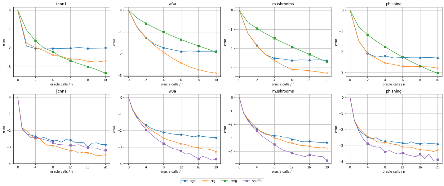
Figure 1: Comparison of the evolution of the relative error for different optimizers on $\ell_{2}$-regularized logistic regression problems using the datasets ijcnn1, w8a, mushrooms and phishing. The top row compares SGD (blue), SRG (orange), and SVRG (green), all with constant step size. The bottom row compares SGD (blue), SRG (orange), and SGD with shuffling (purple), all using decreasing step sizes.

5 Experiments

In this section, we experiment with SRG on $\ell_{2}$-regularized logistic regression problems. In this case, the functions $f_{i}$ are given by:

$$f_{i}(x)\coloneqq\log{(1+\exp{(-y_{i}a_{i}^{T}x)})}+\frac{\mu}{2}\left\lVert x\right\rVert_{2}^{2}$$

where $y_{i}\in\{0,1\}$ is the label of data point $a_{i}\in\mathbb{R}^{d}$. It is not hard to show that each $f_{i}$ is convex and $L_{i}=0.25\left\lVert a_{i}\right\rVert_{2}^{2}+\mu$ smooth. Their average $F$ is also $\mu$-strongly convex.

We experiment with four datasets from LIBSVM (Chang & Lin, 2011): ijcnn1, w8a, mushrooms, and phishing. We start by normalizing the data points $(a_{i})_{i=1}^{n}$ so that $\left\lVert a_{i}\right\rVert_{2}=1$ for all $i\in[n]$. This makes all the $f_{i}$ $L$-smooth with $L=0.25+\mu$. As is standard for regularized logistic regression, we take $\mu=\frac{1}{n}$. We conduct two sets of experiments: one set using a constant step size, and another using decreasing step sizes. In both cases we evaluate the performance of the algorithms by tracking the relative error $\frac{\left\lVert x_{k}-x^{*}\right\rVert_{2}^{2}}{\left\lVert x_{0}-x^{*}\right\rVert_{2}^{2}}$. For all experiments, we sample the indices without replacement using a batch size of $128$. Finally, we use the same step size across all algorithms for each dataset to fairly compare their performance. We give more details on the step sizes we use in the supplementary material.

The results of the experiments with constant step-size can be seen on the top row of Figure 1. We compare SRG with SGD on the one hand and SVRG on the other. We observe that SRG consistently outperforms SGD, reaching solutions that are about an order of magnitude more accurate. We also notice that SRG extends the range of accuracies on which SGD dominates SVRG. Eventually, SVRG outperforms both SGD and SRG, but our results show that SRG allows reaching solutions of moderate accuracy more quickly.

The bottom row of Figure 1 shows the results of the experiments where we use decreasing step-sizes. Here we compare SRG with SGD as well as SGD with random shuffling. SGD with random shuffling has attracted a lot of attention recently, and many analyses have been developed that show its superior performance, see for example (Ahn et al., 2020). Our results confirm this as SGD with shuffling outperforms both SGD and SRG. We still see however that SRG converges slightly faster than SGD, as our analysis suggests.

While the empirical results we present here are positive but not impressive, we would like to point out that the improvement of SRG over SGD depends directly on the ratio $r=\sigma^{2}/\sigma^{2}_{*}$. In particular, if $\sigma_{*}^{2}=\sigma^{2}$, then we should not expect any improvement. For the experiments in Figure 1, $r$ is in the range $[5,10]$. One can construct artificial examples in which this ratio is very large, which we do in the supplementary material, leading to significant improvements. It is however still unclear how often such cases are encountered in practice. We hope to explore this question more in future work.

Appendix A Standard results

Lemma 5.

Under Assumptions 2 and 3, we have:

$$\frac{1}{n}\sum_{i=1}^{n}\left\lVert\nabla f_{i}(x)-\nabla f_{i}(x^{*})\right\rVert_{2}^{2}\leq 2L\left[F(x)-F(x^{*})\right]$$

Proof.

By Assumptions 2 and 3, and Theorem 2.1.5 in (Nesterov, 2004) we have for all $i\in[n]$:

$$f_{i}(x)\leq f_{i}(x^{*})+\langle\nabla f_{i}(x^{*}),x-x^{*}\rangle+\frac{1}{2L}\left\lVert\nabla f_{i}(x)-\nabla f_{i}(x^{*})\right\rVert_{2}^{2}$$

Rearranging gives:

$$\left\lVert\nabla f_{i}(x)-\nabla f_{i}(x^{*})\right\rVert_{2}^{2}\leq 2L\left[f_{i}(x)-f_{i}(x^{*})-\langle\nabla f_{i}(x^{*}),x-x^{*}\rangle\right]$$

Averaging over $i\in[n]$ and noticing that $\frac{1}{n}\sum_{i=1}^{n}\nabla f_{i}(x^{*})=\nabla F(x^{*})=0$, we get the result. ∎

Proposition 3.

(Young’s inequality, Peter-Paul inequality) Let $a,b,c\in\mathbb{R}^{d}$. Then for all $\beta,\gamma,\delta>0$ we have:

$$\left\lVert a+b\right\rVert_{2}^{2} \leq(1+\beta)\left\lVert a\right\rVert_{2}^{2}+(1+\beta^{-1})\left\lVert b\right\rVert_{2}^{2}$$

$$\left\lVert a+b+c\right\rVert_{2}^{2} \leq(1+\beta+\gamma)\left\lVert a\right\rVert_{2}^{2}+(1+\beta^{-1}+\delta)\left\lVert b\right\rVert_{2}^{2}+(1+\gamma^{-1}+\delta^{-1})\left\lVert c\right\rVert_{2}^{2}$$

Proof.

We prove the first statement. The second follows from a similar argument. We have for $x,y\in\mathbb{R}$:

$$\beta x^{2}-2xy+\beta^{-1}y^{2}=\left(\sqrt{\beta}x-\sqrt{\beta^{-1}}y\right)^{2}\geq 0\Rightarrow 2xy\leq\beta x^{2}+\beta^{-1}y^{2}$$

$$\beta x^{2}+2xy+\beta^{-1}y^{2}=\left(\sqrt{\beta}x+\sqrt{\beta^{-1}}y\right)^{2}\geq 0\Rightarrow-2xy\leq\beta x^{2}+\beta^{-1}y^{2}$$

Therefore:

$$2\lvert xy\rvert\leq\beta x^{2}+\beta^{-1}y^{2}$$

Now by Cauchy-Schwarz inequality:

$$\left\lVert a+b\right\rVert_{2}^{2} =\left\lVert a\right\rVert_{2}^{2}+2\langle a,b\rangle+\left\lVert b\right\rVert_{2}^{2}$$

$$\leq\left\lVert a\right\rVert_{2}^{2}+2\lvert\langle a,b\rangle\rvert+\left\lVert b\right\rVert_{2}^{2}$$

$$\leq\left\lVert a\right\rVert_{2}^{2}+2\left\lVert a\right\rVert_{2}\left\lVert b\right\rVert_{2}+\left\lVert b\right\rVert_{2}^{2}$$

$$\leq(1+\beta)\left\lVert a\right\rVert_{2}^{2}+(1+\beta^{-1})\left\lVert b\right\rVert_{2}^{2}$$

∎

Appendix B Missing proofs

B.1 Proof of Lemma 3

Proof.

Taking expectation with respect to $(i_{k},b_{k})$ conditional on $(i_{t},b_{t})_{t=1}^{k-1}$ we have:

$$\mathbb{E}\left[\sum_{i=1}^{n}\left\lVert g_{k+1}^{i}-\nabla f_{i}(x^{*})\right\rVert_{2}^{2}\right]$$

$$=\sum_{j=1}^{n}\mathbb{P}(i_{k}=j)\biggl{[}\mathbb{P}(b_{k}=0\mid i_{k}=j)\left(\sum_{i=1}^{n}\left\lVert g_{k}^{i}-\nabla f_{i}(x^{*})\right\rVert_{2}^{2}\right)$$

$$\quad+\mathbb{P}(b_{k}=1\mid i_{k}=j)\left(\sum_{\begin{subarray}{c}i=1\\ i\neq j\end{subarray}}^{n}\left\lVert g_{k}^{i}-\nabla f_{i}(x^{*})\right\rVert_{2}^{2}+\left\lVert\nabla f_{j}(x_{k})-\nabla f_{j}(x^{*})\right\rVert_{2}^{2}\right)\biggl{]}$$

$$=\sum_{j=1}^{n}p_{k}^{j}\left[\left(1-\frac{\varepsilon_{k}}{p_{k}^{j}}\right)\sum_{i=1}^{n}\left\lVert g_{k}^{i}-\nabla f_{i}(x^{*})\right\rVert_{2}^{2}+\frac{\varepsilon_{k}}{p_{k}^{j}}\left(\sum_{\begin{subarray}{c}i=1\\ i\neq j\end{subarray}}^{n}\left\lVert g_{k}^{i}-\nabla f_{i}(x^{*})\right\rVert_{2}^{2}+\left\lVert\nabla f_{j}(x_{k})-\nabla f_{j}(x^{*})\right\rVert_{2}^{2}\right)\right]$$

$$=\left(1-\varepsilon_{k}\right)\sum_{i=1}^{n}\left\lVert g_{k}^{i}-\nabla f_{i}(x^{*})\right\rVert_{2}^{2}+\varepsilon_{k}\sum_{i=1}^{n}\left\lVert\nabla f_{i}(x_{k})-\nabla f_{i}(x^{*})\right\rVert_{2}^{2}$$

$$\leq\left(1-\varepsilon_{k}\right)\sum_{i=1}^{n}\left\lVert g_{k}^{i}-\nabla f_{i}(x^{*})\right\rVert_{2}^{2}+2Ln\varepsilon_{k}\left[F(x_{k})-F(x^{*})\right]$$

where the second and third lines follow from the update of Algorithm 1, and the last line follows from Lemma 5. ∎

B.2 Proof of Lemma 4

Proof.

Taking expectation with respect to $(i_{k},b_{k})$ conditional on $(i_{t},b_{t})_{t=1}^{k-1}$ we have:

$$\mathbb{E}\left[\left\lVert\frac{1}{np_{k}^{i_{k}}}\nabla f_{i_{k}}(x_{k})\right\rVert_{2}^{2}\right]=\frac{1}{n^{2}}\sum_{i=1}^{n}\frac{1}{p_{k}^{i}}\left\lVert\nabla f_{i}(x_{k})\right\rVert_{2}^{2}$$

Now by Proposition 3:

$$\sum_{i=1}^{n}\frac{1}{p_{k}^{i}}\left\lVert\nabla f_{i}(x_{k})\right\rVert_{2}^{2} =\sum_{i=1}^{n}\frac{1}{p_{k}^{i}}\left\lVert\nabla f_{i}(x_{k})-\nabla f_{i}(x^{*})+\nabla f_{i}(x^{*})-g_{k}^{i}+g_{k}^{i}\right\rVert_{2}^{2}$$

$$\leq(1+\beta+\gamma)\sum_{i=1}^{n}\frac{1}{p_{k}^{i}}\left\lVert\nabla f_{i}(x_{k})-\nabla f_{i}(x^{*})\right\rVert_{2}^{2}$$

$$\quad+(1+\beta^{-1}+\delta)\sum_{i=1}^{n}\frac{1}{p_{k}^{i}}\left\lVert g_{k}^{i}-\nabla f_{i}(x^{*})\right\rVert_{2}^{2}$$

$$\quad+(1+\gamma^{-1}+\delta^{-1})\sum_{i=1}^{n}\frac{1}{p_{k}^{i}}\left\lVert g_{k}^{i}\right\rVert_{2}^{2}$$

Let us bound each of the three terms. The first can be bound using $p_{k}\geq\varepsilon_{k}$ and Lemma 5:

$$\sum_{i=1}^{n}\frac{1}{p_{k}^{i}}\left\lVert\nabla f_{i}(x_{k})-\nabla f_{i}(x^{*})\right\rVert_{2}^{2} \leq\frac{1}{\varepsilon_{k}}\sum_{i=1}^{n}\left\lVert\nabla f_{i}(x_{k})-\nabla f_{i}(x^{*})\right\rVert_{2}^{2}\leq\frac{2Ln}{\varepsilon_{k}}\left[F(x_{k})-F(x^{*})\right]$$

The second is easily bound using $p_{k}\geq\varepsilon_{k}$:

$$\sum_{i=1}^{n}\frac{1}{p_{k}^{i}}\left\lVert g_{k}^{i}-\nabla f_{i}(x^{*})\right\rVert_{2}^{2}\leq\frac{1}{\varepsilon_{k}}\sum_{i=1}^{n}\left\lVert g_{k}^{i}-\nabla f_{i}(x^{*})\right\rVert_{2}^{2}$$

Finally, the third term can be bound as:

$$\sum_{i=1}^{n}\frac{1}{p_{k}^{i}}\left\lVert g_{k}^{i}\right\rVert_{2}^{2}$$

$$\leq(1+2n\varepsilon_{k})\left(\sum_{i=1}^{n}\left\lVert g_{k}^{i}\right\rVert_{2}\right)^{2}$$

$$\leq(1+2n\varepsilon_{k})\left(\sum_{i=1}^{n}\left\lVert g_{k}^{i}-\nabla f_{i}(x^{*})\right\rVert_{2}+\sum_{i=1}^{n}\left\lVert\nabla f_{i}(x^{*})\right\rVert_{2}\right)^{2}$$

$$\leq(1+2n\varepsilon_{k})(1+\eta)\left(\sum_{i=1}^{n}\left\lVert g_{k}^{i}-\nabla f_{i}(x_{k})\right\rVert_{2}\right)^{2}+(1+2n\varepsilon_{k})(1+\eta^{-1})\left(\sum_{i=1}^{n}\left\lVert\nabla f_{i}(x^{*})\right\rVert_{2}\right)^{2}$$

$$\leq(1+2n\varepsilon_{k})(1+\eta)n\sum_{i=1}^{n}\left\lVert g_{k}^{i}-\nabla f_{i}(x^{*})\right\rVert_{2}^{2}+(1+2n\varepsilon_{k})(1+\eta^{-1})n^{2}\sigma_{*}^{2}$$

$$\leq 2n(1+\eta)\sum_{i=1}^{n}\left\lVert g_{k}^{i}-\nabla f_{i}(x^{*})\right\rVert_{2}^{2}+(1+2n\varepsilon_{k})(1+\eta^{-1})n^{2}\sigma_{*}^{2}$$

$$\leq(1+\eta)\frac{1}{\varepsilon_{k}}\sum_{i=1}^{n}\left\lVert g_{k}^{i}-\nabla f_{i}(x^{*})\right\rVert_{2}^{2}+(1+\eta^{-1})(1+2n\varepsilon_{k})n^{2}\sigma_{*}^{2}$$

Where the second line follows from Proposition 2, the third from the triangle inequality, and the fourth by Proposition 3. The fifth line follows from the definition of $\sigma^{2}_{*}$ in section 4 and an application of Cauchy-Schwarz inequality. Let $v$ be the vector whose $i^{th}$ component is $\left\lVert g_{k}^{i}-\nabla f_{i}(x^{*})\right\rVert_{2}$ and let $1_{n}$ be the vector of ones. Then:

$$\left(\sum_{i=1}^{n}\left\lVert g_{k}^{i}-\nabla f_{i}(x^{*})\right\rVert_{2}\right)^{2}=\lvert\langle 1_{n},v\rangle\rvert^{2}\leq\left\lVert 1_{n}\right\rVert_{2}^{2}\left\lVert v\right\rVert_{2}^{2}=n\sum_{i=1}^{n}\left\lVert g_{k}^{i}-\nabla f_{i}(x^{*})\right\rVert_{2}^{2}$$

Finally, lines six and seven follow from the inequality $\varepsilon_{k}\leq 1/2n$. Combining the three bounds yields the result. ∎

B.3 Proof of Theorem 1

Proof.

Recall that we are studying the one-step evolution of the Lyapunov function:

$$T^{k}=T(x_{k},(g_{k}^{i})_{i=1}^{n})\coloneqq\frac{\alpha_{k}}{n\varepsilon_{k}}\frac{a}{L}\sum_{i=1}^{n}\left\lVert g_{k}^{i}-\nabla f_{i}(x^{*})\right\rVert_{2}^{2}+\left\lVert x_{k}-x^{*}\right\rVert_{2}^{2}$$

and that we are assuming (i) $\alpha_{k}/\varepsilon_{k}$is constant. (ii) $\varepsilon_{k}\in(0,1/2n]$. (iii) $\alpha_{k}\leq n\varepsilon_{k}/20L$.

All the expectations in this proof are with respect to $(i_{k},b_{k})$ and are conditional on $(i_{t},b_{t})_{t=0}^{k-1}$. Since $\alpha_{k}/\varepsilon_{k}$ is constant, Lemma 3 immediately gives us a bound on the first term of $\mathbb{E}\left[T^{k+1}\right]$.

The second term of $\mathbb{E}\left[T^{k+1}\right]$ expands as:

$$\mathbb{E}\left[\left\lVert x_{k+1}-x^{*}\right\rVert_{2}^{2}\right] =\mathbb{E}\left[\left\lVert x_{k}-\alpha_{k}\frac{1}{np_{k}^{i_{k}}}\nabla f_{i_{k}}(x_{k})-x^{*}\right\rVert_{2}^{2}\right]$$

$$=\left\lVert x_{k}-x^{*}\right\rVert_{2}^{2}-2\alpha_{k}\langle\mathbb{E}\left[\frac{1}{np_{k}^{i_{k}}}\nabla f_{i_{k}}(x_{k})\right],x_{k}-x^{*}\rangle+\alpha_{k}^{2}\mathbb{E}\left[\left\lVert\frac{1}{np_{k}^{i_{k}}}\nabla f_{i_{k}}(x_{k})\right\rVert_{2}^{2}\right]$$

$$=\left\lVert x_{k}-x^{*}\right\rVert_{2}^{2}-2\alpha_{k}\langle\nabla F(x_{k}),x_{k}-x^{*}\rangle+\alpha_{k}^{2}\mathbb{E}\left[\left\lVert\frac{1}{np_{k}^{i_{k}}}\nabla f_{i_{k}}(x_{k})\right\rVert_{2}^{2}\right]$$

$$\leq(1-\alpha_{k}\mu)\left\lVert x_{k}-x^{*}\right\rVert_{2}-2\alpha_{k}\left[F(x_{k})-F(x^{*})\right]+\alpha_{k}^{2}\mathbb{E}\left[\left\lVert\frac{1}{np_{k}^{i_{k}}}\nabla f_{i_{k}}(x_{k})\right\rVert_{2}^{2}\right]$$

where in the last line we use Assumption 1 (strong-convexity of $F$). Since we are assuming $\varepsilon_{k}\in(0,1/2n]$, we can apply Lemma 4 to bound the last term above. Combining the resulting bound with the one on the first term we get:

$$\mathbb{E}\left[T^{k+1}\right] \leq\left(1-\varepsilon_{k}+\frac{D_{1}\alpha_{k}L}{na}\right)\frac{\alpha_{k}}{n\varepsilon_{k}}\frac{a}{L}\sum_{i=1}^{n}\left\lVert g_{k}^{i}-\nabla f_{i}(x^{*})\right\rVert_{2}^{2}+\left(1-\alpha_{k}\mu\right)\left\lVert x_{k}-x^{*}\right\rVert_{2}^{2}$$

$$\quad+D_{3}(1+2n\varepsilon_{k})\alpha_{k}^{2}\sigma_{*}^{2}$$

$$\quad+\frac{2\alpha_{k}L}{n\varepsilon_{k}}\left(D_{2}\alpha_{k}+\frac{an\varepsilon_{k}}{L}-\frac{n\varepsilon_{k}}{L}\right)\left[F(x_{k})-F(x^{*})\right]$$

To ensure that the last parenthesis is not positive, we need:

$$\alpha_{k}\leq\frac{(1-a)}{D_{2}}\frac{n\varepsilon_{k}}{L}$$ (11)

Assuming $\alpha_{k}$ satisfies this condition, and replacing in the first parenthesis we get:

$$1-\varepsilon_{k}+\frac{D_{1}\alpha_{k}L}{na}\leq 1-\alpha_{k}\left(\frac{D_{2}}{1-a}-\frac{D_{1}}{a}\right)\frac{L}{n}$$

Now:

$$\min\left\{\left(\frac{D_{2}}{1-a}-\frac{D_{1}}{a}\right)\frac{L}{n},\mu\right\}\leq\min\left\{\left(\frac{D_{2}}{1-a}-\frac{D_{1}}{a}\right),1\right\}\zeta$$

where:

$$\zeta\coloneqq\min\left\{\frac{L}{n},\mu\right\}$$

So that, assuming (11) holds, our upper bound on $\mathbb{E}\left[T^{k+1}\right]$ is itself upper bounded by:

$$\mathbb{E}\left[T^{k+1}\right]\leq\left(1-\alpha_{k}\min\left\{\left(\frac{D_{2}}{1-a}-\frac{D_{1}}{a}\right),1\right\}\zeta\right)T^{k}+D_{3}(1+2n\varepsilon_{k})\alpha_{k}^{2}\sigma_{*}^{2}$$

It remains to choose the parameters $\beta,\gamma,\delta,\eta>0$, and the parameter $a>0$ so as to minimize this upper bound while maximizing the step size in (11). First however, note that we have the constraint $a<1$ so that the step size can be allowed to be positive in (11). Furthermore, we choose to impose $D_{3}=2$ since this is also the leading factor in the analogous term in the analysis of SGD (Gower et al., 2019).

These considerations lead us to the following constrained optimization problem:

$$\max_{a,\beta,\gamma,\delta,\eta}\quad \frac{(1-a)}{D_{2}}$$

subject to: $$\frac{D_{2}}{1-a}-\frac{D_{1}}{a}\geq 1$$

$$D_{3}\leq 2$$

$$0<a<1$$

$$\beta,\gamma,\delta,\eta>0$$

which we solve numerically to find the feasible point:

$$a=0.673,\ \beta=1.028,\ \gamma=4.084,\ \delta=3.973,\ \eta=2.980$$

With this choice of parameters, we get:

$$\mathbb{E}\left[T^{k+1}\right]\leq\left(1-\alpha_{k}\zeta\right)T^{k}+(1+2n\varepsilon_{k})2\alpha_{k}^{2}\sigma_{*}^{2}$$

under the condition:

$$\alpha_{k}\leq\frac{1}{20}\frac{n\varepsilon_{k}}{L}$$

which ensures that (11) holds. ∎

B.4 Proof of Corollary 1

Proof.

Under the assumptions of the corollary, the conditions of Theorem 1 are satisfied for all $k\in\mathbb{N}$. Starting from $\mathbb{E}\left[T^{k}\right]$ and repeatedly applying Theorem 1 we get:

$$\mathbb{E}\left[T^{k}\right] \leq(1-\alpha\zeta)^{k}T^{0}+(1+2n\varepsilon)2\alpha^{2}\sigma_{*}^{2}\sum_{t=0}^{k-1}(1-\alpha\zeta)^{t}$$

$$\leq(1-\alpha\zeta)^{k}T^{0}+(1+2n\varepsilon)2\alpha^{2}\sigma_{*}^{2}\sum_{t=0}^{\infty}(1-\alpha\zeta)^{t}$$

$$=(1-\alpha\rho)^{k}T^{0}+(1+2n\varepsilon)\frac{2\alpha\sigma_{*}^{2}}{\zeta}$$

∎

B.5 Proof of Corollary 2

Proof.

The choices of $\varepsilon_{k}$, $\alpha_{k}$, and of the constants $c$ and $k_{0}$ are such that: (i) $\alpha_{k}/\varepsilon_{k}$is constant. (ii) $\alpha_{k}\leq n\varepsilon_{k}/20L$for all $k\in\mathbb{N}$. (iii) $\alpha_{k}$, and therefore $\varepsilon_{k}$, is decreasing for all $k\in\mathbb{N}$. (iv) $\varepsilon_{0}=\frac{1}{2n}$. Therefore, the conditions of Theorem 1 hold for all $k\in\mathbb{N}$. Fix $k\in\mathbb{N}$. We have by Theorem 1 for any $t\in[k-1]\cup\{0\}$:

$$\mathbb{E}\left[T^{t+1}\right] \leq(1-\alpha_{t}\zeta)\mathbb{E}\left[T^{t}\right]+(1+2n\varepsilon_{t})2\alpha_{t}^{2}\sigma_{*}^{2}$$

$$=\frac{c+(t+k_{0}-1)(t+k_{0}+1)}{c+(t+k_{0})(t+k_{0}+2)}\mathbb{E}\left[T^{t}\right]+(1+2n\varepsilon_{t})2\alpha_{t}^{2}\sigma_{*}^{2}$$

multiplying both sides by $\left[c+(t+k_{0})(t+k_{0}+2)\right]$ and noticing that:

$$\left[c+(t+k_{0})(t+k_{0}+2)\right]\alpha_{t}^{2}=\frac{\left[2(t+k_{0})+1\right]^{2}}{\left[c+(t+k_{0})(t+k_{0}+2)\right]}\leq 4$$

we get:

$$\left[c+(t+k_{0})(t+k_{0}+2)\right]\mathbb{E}\left[T^{t+1}\right]-\left[c+(t+k_{0}-1)(t+k_{0}+1)\right]\mathbb{E}\left[T^{t}\right]\leq(1+2n\varepsilon_{t})8\sigma_{*}^{2}$$

summing the $k$ inequalities for $t\in[k-1]\cup\{0\}$ and noticing that the left side is a telescoping sum we obtain:

$$\left[c+(k+k_{0})(k+k_{0}+2)\right]\mathbb{E}\left[T^{k}\right]-\left[c+(k_{0}-1)(k_{0}+1)\right]T^{0}\leq 8k\sigma_{*}^{2}+16n\sigma_{*}^{2}\sum_{t=0}^{k-1}\varepsilon_{t}$$

Let us now bound the last term:

$$16n\sigma_{*}^{2}\sum_{t=0}^{k-1}\varepsilon_{t} =320L\sigma_{*}^{2}\sum_{t=0}^{k-1}\alpha_{t}$$

$$=\frac{320L\sigma_{*}^{2}}{\zeta}\sum_{t=0}^{k-1}\frac{2(t+k_{0})+1}{\left[c+(t+k_{0})(t+k_{0}+2)\right]}$$

$$\leq\frac{320L\sigma_{*}^{2}}{\zeta}\int_{-1}^{k-1}\frac{2(x+k_{0})+1}{\left[c+(x+k_{0})(x+k_{0}+2)\right]}\,dx$$

$$\leq\frac{320L\sigma_{*}^{2}}{\zeta}\int_{-1}^{k-1}\frac{2(x+k_{0}+1)}{\left[c+(x+k_{0})(x+k_{0}+2)\right]}\,dx$$

$$=\frac{320L\sigma_{*}^{2}}{\zeta}\log{\frac{\left[c+(k+k_{0}-1)(k+k_{0}+1)\right]}{\left[c+(k_{0}-1)(k_{0}+1)\right]}}$$

where the first line follows from the definition of $\varepsilon_{t}$, and the third line follows from the fact that the integrand is decreasing over the domain of integration. Using this bound and rearranging:

$$\mathbb{E}\left[T^{k}\right] \leq\frac{\left[c+(k_{0}-1)(k_{0}+1)\right]}{\left[c+(k+k_{0})(k+k_{0}+2)\right]}T^{0}+\frac{8k\sigma_{*}^{2}}{\left[c+(k+k_{0})(k+k_{0}+2)\right]}$$

$$\quad+\frac{320L\sigma_{*}^{2}}{\zeta}\frac{1}{\left[c+(k+k_{0})(k+k_{0}+2)\right]}\log{\frac{\left[c+(k+k_{0}-1)(k+k_{0}+1)\right]}{\left[c+(k_{0}-1)(k_{0}+1)\right]}}$$

$$=O\left(\frac{T^{0}+\sigma_{*}^{2}\log{k}}{k^{2}}\right)+O\left(\frac{\sigma_{*}^{2}}{k}\right)$$

∎

Appendix C Details of experiments

In this section we give more details on the experiments presented in section 5.

Batch size:

Our analysis is for the case where the batch size is equal to 1. We would have therefore ideally liked to run the experiments with a unit batch size. This is however extremely slow, so we used instead a batch size of $m=128$ sampled without replacement.

Step sizes:

To make a fair comparison between the algorithms, we use the same step size sequence across them for a given dataset. Define:

$$\mathcal{L}=\frac{n-m}{m(n-1)}L_{max}+\frac{n(m-1)}{m(n-1)}L$$

where $L_{max}=\max_{i\in[n]}L_{i}$ where $L_{i}$ is the smoothness constant of $f_{i}$, $L$ is the smoothness constant of $F$, and $m$ is the batch size.

For the constant step size experiments, we use SGD as a reference, and use the maximum step size allowable in its analysis in (Gower et al., 2019), which is given by:

$$\alpha=\frac{1}{2\mathcal{L}}$$

Similarly, for the decreasing step size experiments, we use the step sizes:

$$\alpha_{k}=\frac{2(k+k_{0})+1}{\left[c+(k+k_{0})(k+k_{0}+2)\right]\mu}$$

where:

$$k_{0} =\frac{4\mathcal{L}}{\mu}-2$$

$$c =\frac{2\mathcal{L}}{\mu}$$

Algorithm specific parameters:

For SRG, we initialize $g_{0}^{i}=0$ for all $i\in[n]$, and we always update $g_{k}^{i_{k}}$, i.e. we do not sample a Bernoulli to decide whether the update occurs or not, as we believe that the added Bernoulli is only an artifact of the analysis. Furthermore, as the indices are sampled without replacement, the naive importance sampling estimator is biased. We use the mini-batch estimator introduced in (El Hanchi & Stephens, 2020) which corrects for this bias. For the constant step size experiments, we set $\varepsilon_{k}=\varepsilon=1/2n$, while for the ones using decreasing step sizes, we set $\varepsilon_{k}=\mathcal{L}\alpha_{k}/n$

For SVRG, we use its loopless version (Hofmann et al., 2015) to avoid the stairlike behavior of the convergence plot of SVRG. We use a full update probability of $q=m/n$ so that the expected number of gradient evaluations per iteration is three times that of SGD, the same ratio that we would expect from running standard SVRG and SGD with a unit batch size.

For SGD with random shuffling, we sample a fresh permutation at the beginning of each epoch.

Figure:

Figure 1 shows the evolution of the log relative error:

$$\log_{10}\left(\frac{\left\lVert x_{k}-x^{*}\right\rVert_{2}^{2}}{\left\lVert x_{0}-x^{*}\right\rVert_{2}^{2}}\right)$$

For each algorithm and each dataset, we run the algorithm ten times and plot the average of the results.

Appendix D Synthetic experiment

In this section, we compare SRG and SGD on a synthetic dataset. Our theoretical analysis suggests that the improvement of SRG over SGD is proportional to the ratio $r=\sigma^{2}/\sigma_{*}^{2}$. Here we construct an artificial example in which this ratio is large ($r\approx 50$), compared to $r\in[5,10]$ for the experiments in section 5.

We do this by generating a synthetic dataset as follows:

• generate a $1000\times 10$ features matrix $A$ randomly with $a_{ij}\sim\mathcal{N}(0,1)$.

• generate a weight vector $w$ randomly with $w_{i}\sim\mathcal{N}(0,1)$.

• generate the target values randomly as:

  $$y_{i}=w^{T}a_{i}+\varepsilon_{i}$$

  where each $\varepsilon_{i}$ is an independent standard Cauchy random variable.

We then fit a linear regression model with the mean squared error loss using SGD and SRG. We use a batch size of $1$, and a constant step size $\alpha=1/2L$ for both. For SRG we use $\varepsilon_{k}=\varepsilon=1/2n$, and initialize $g_{0}^{i}=0$. The results are displayed in Figure 2. We ran each algorithm a hundred times and plotted the average of the results. The left plot shows the evolution of the log relative error, while the right one shows the evolution of the log of the variance of the gradient estimator $\sigma^{2}(x_{k},1/n)$ and $\sigma^{2}(x_{k},p_{k})$ respectively for SGD and SRG. We see that SRG reaches solution that are approximately two orders of magnitude more accurate than SGD, which is what we expect from the value of the ratio $r\approx 50$. As pointed out in section 5, it is not clear how often such large values for the ratio $r$ are encountered in practice, but our experiments confirm that substantial gains can be achieved if it is large enough.

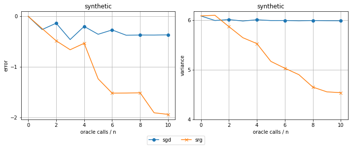
Figure 2: Comparison of the evolution of the relative error (left) and the variance of the gradient estimator (right) for SGD and SRG applied to the synthetic dataset described in section D.

References

• Agarwal & Bottou (2015) Agarwal, A. and Bottou, L. A Lower Bound for the Optimization of Finite Sums. In International Conference on Machine Learning, pp. 78–86. PMLR, June 2015.
• Ahn et al. (2020) Ahn, K., Yun, C., and Sra, S. SGD with shuffling: optimal rates without component convexity and large epoch requirements. Advances in Neural Information Processing Systems, 33, 2020.
• Alain et al. (2016) Alain, G., Lamb, A., Sankar, C., Courville, A., and Bengio, Y. Variance Reduction in SGD by Distributed Importance Sampling. arXiv:1511.06481 [cs, stat], April 2016.
• Allen-Zhu (2018) Allen-Zhu, Z. Katyusha: The First Direct Acceleration of Stochastic Gradient Methods. Journal of Machine Learning Research, 18(221):1–51, 2018.
• Arjevani (2017) Arjevani, Y. Limitations on Variance-Reduction and Acceleration Schemes for Finite Sums Optimization. Advances in Neural Information Processing Systems, 30:3540–3549, 2017.
• Borsos et al. (2018) Borsos, Z., Krause, A., and Levy, K. Y. Online Variance Reduction for Stochastic Optimization. In Conference On Learning Theory, pp.  324–357. PMLR, July 2018.
• Borsos et al. (2019) Borsos, Z., Curi, S., Levy, K. Y., and Krause, A. Online Variance Reduction with Mixtures. In International Conference on Machine Learning, pp. 705–714. PMLR, May 2019.
• Bouchard et al. (2016) Bouchard, G., Trouillon, T., Perez, J., and Gaidon, A. Online Learning to Sample. arXiv:1506.09016 [cs, math, stat], March 2016.
• Canevet et al. (2016) Canevet, O., Jose, C., and Fleuret, F. Importance Sampling Tree for Large-scale Empirical Expectation. In International Conference on Machine Learning, pp. 1454–1462. PMLR, June 2016.
• Chang & Lin (2011) Chang, C.-C. and Lin, C.-J. Libsvm: A library for support vector machines. ACM Trans. Intell. Syst. Technol., 2(3), May 2011.
• Cormen et al. (2009) Cormen, T. H., Leiserson, C. E., Rivest, R. L., and Stein, C. Introduction to Algorithms. MIT Press, July 2009.
• Csiba & Richtárik (2018) Csiba, D. and Richtárik, P. Importance Sampling for Minibatches. Journal of Machine Learning Research, 19(27):1–21, 2018.
• Defazio (2016) Defazio, A. A Simple Practical Accelerated Method for Finite Sums. Advances in Neural Information Processing Systems, 29:676–684, 2016.
• Defazio & Bottou (2019) Defazio, A. and Bottou, L. On the Ineffectiveness of Variance Reduced Optimization for Deep Learning. Advances in Neural Information Processing Systems, 32:1755–1765, 2019.
• Defazio et al. (2014) Defazio, A., Bach, F., and Lacoste-Julien, S. SAGA: A Fast Incremental Gradient Method With Support for Non-Strongly Convex Composite Objectives. Advances in Neural Information Processing Systems, 27:1646–1654, 2014.
• El Hanchi & Stephens (2020) El Hanchi, A. and Stephens, D. Adaptive Importance Sampling for Finite-Sum Optimization and Sampling with Decreasing Step-Sizes. Advances in Neural Information Processing Systems, 33, 2020.
• Gower et al. (2019) Gower, R. M., Loizou, N., Qian, X., Sailanbayev, A., Shulgin, E., and Richtárik, P. SGD: General Analysis and Improved Rates. In International Conference on Machine Learning, pp. 5200–5209. PMLR, May 2019.
• Goyal et al. (2018) Goyal, P., Dollár, P., Girshick, R., Noordhuis, P., Wesolowski, L., Kyrola, A., Tulloch, A., Jia, Y., and He, K. Accurate, Large Minibatch SGD: Training ImageNet in 1 Hour. arXiv:1706.02677 [cs], April 2018.
• Hofmann et al. (2015) Hofmann, T., Lucchi, A., Lacoste-Julien, S., and McWilliams, B. Variance Reduced Stochastic Gradient Descent with Neighbors. Advances in Neural Information Processing Systems, 28:2305–2313, 2015.
• Johnson & Zhang (2013) Johnson, R. and Zhang, T. Accelerating Stochastic Gradient Descent using Predictive Variance Reduction. Advances in Neural Information Processing Systems, 26:315–323, 2013.
• Johnson & Guestrin (2018) Johnson, T. B. and Guestrin, C. Training Deep Models Faster with Robust, Approximate Importance Sampling. Advances in Neural Information Processing Systems, 31:7265–7275, 2018.
• Katharopoulos & Fleuret (2018) Katharopoulos, A. and Fleuret, F. Not All Samples Are Created Equal: Deep Learning with Importance Sampling. In International Conference on Machine Learning, pp. 2525–2534. PMLR, July 2018.
• Lan & Zhou (2018) Lan, G. and Zhou, Y. An optimal randomized incremental gradient method. Mathematical Programming, 171(1):167–215, September 2018.
• Lan et al. (2019) Lan, G., Li, Z., and Zhou, Y. A unified variance-reduced accelerated gradient method for convex optimization. Advances in Neural Information Processing Systems, 32:10462–10472, 2019.
• Lin et al. (2018) Lin, H., Mairal, J., and Harchaoui, Z. Catalyst Acceleration for First-order Convex Optimization: from Theory to Practice. Journal of Machine Learning Research, 18(212):1–54, 2018.
• Loshchilov & Hutter (2015) Loshchilov, I. and Hutter, F. Online Batch Selection for Faster Training of Neural Networks. November 2015.
• Ma et al. (2018) Ma, S., Bassily, R., and Belkin, M. The Power of Interpolation: Understanding the Effectiveness of SGD in Modern Over-parametrized Learning. In International Conference on Machine Learning, pp. 3325–3334. PMLR, July 2018.
• Moulines & Bach (2011) Moulines, E. and Bach, F. Non-Asymptotic Analysis of Stochastic Approximation Algorithms for Machine Learning. Advances in Neural Information Processing Systems, 24:451–459, 2011.
• Namkoong et al. (2017) Namkoong, H., Sinha, A., Yadlowsky, S., and Duchi, J. C. Adaptive Sampling Probabilities for Non-Smooth Optimization. In International Conference on Machine Learning, pp. 2574–2583. PMLR, July 2017.
• Needell et al. (2014) Needell, D., Ward, R., and Srebro, N. Stochastic Gradient Descent, Weighted Sampling, and the Randomized Kaczmarz algorithm. Advances in Neural Information Processing Systems, 27:1017–1025, 2014.
• Nemirovski et al. (2009) Nemirovski, A., Juditsky, A., Lan, G., and Shapiro, A. Robust Stochastic Approximation Approach to Stochastic Programming. SIAM Journal on Optimization, 19(4):1574–1609, January 2009.
• Nemirovsky & Yudin (1983) Nemirovsky, A. S. and Yudin, D. B. Problem Complexity and Method Efficiency in Optimization. John Wiley, Chichester, 1983.
• Nesterov (1983) Nesterov, Y. A method for solving the convex programming problem with convergence rate $o(1/k^{2})$. Proceedings of the USSR Academy of Sciences, 269:543–547, 1983.
• Nesterov (2004) Nesterov, Y. Introductory Lectures on Convex Optimization: A Basic Course. Applied Optimization. Springer US, 2004.
• Nesterov (2018) Nesterov, Y. Lectures on Convex Optimization. Springer Optimization and Its Applications. Springer International Publishing, 2 edition, 2018.
• Nguyen et al. (2018) Nguyen, L., Nguyen, P. H., Dijk, M., Richtarik, P., Scheinberg, K., and Takac, M. SGD and Hogwild! Convergence Without the Bounded Gradients Assumption. In International Conference on Machine Learning, pp. 3750–3758. PMLR, July 2018.
• Nguyen et al. (2017) Nguyen, L. M., Liu, J., Scheinberg, K., and Takáč, M. SARAH: A Novel Method for Machine Learning Problems Using Stochastic Recursive Gradient. In International Conference on Machine Learning, pp. 2613–2621. PMLR, July 2017.
• Pesme et al. (2020) Pesme, S., Dieuleveut, A., and Flammarion, N. On Convergence-Diagnostic based Step Sizes for Stochastic Gradient Descent. In International Conference on Machine Learning, pp. 7641–7651. PMLR, November 2020.
• Robbins & Monro (1951) Robbins, H. and Monro, S. A Stochastic Approximation Method. Annals of Mathematical Statistics, 22(3):400–407, September 1951.
• Roux et al. (2012) Roux, N., Schmidt, M., and Bach, F. A Stochastic Gradient Method with an Exponential Convergence _rate for Finite Training Sets. Advances in Neural Information Processing Systems, 25:2663–2671, 2012.
• Salehi et al. (2017) Salehi, F., Celis, L. E., and Thiran, P. Stochastic Optimization with Bandit Sampling. August 2017.
• Schaul et al. (2015) Schaul, T., Quan, J., Antonoglou, I., and Silver, D. Prioritized Experience Replay. November 2015.
• Schmidt et al. (2017) Schmidt, M., Le Roux, N., and Bach, F. Minimizing finite sums with the stochastic average gradient. Mathematical Programming, 162(1):83–112, March 2017.
• Song et al. (2020) Song, C., Jiang, Y., and Ma, Y. Variance Reduction via Accelerated Dual Averaging for Finite-Sum Optimization. Advances in Neural Information Processing Systems, 33, 2020.
• Stich et al. (2017) Stich, S. U., Raj, A., and Jaggi, M. Safe Adaptive Importance Sampling. Advances in Neural Information Processing Systems, 30:4381–4391, 2017.
• Vaswani et al. (2019a) Vaswani, S., Bach, F., and Schmidt, M. Fast and Faster Convergence of SGD for Over-Parameterized Models and an Accelerated Perceptron. In The 22nd International Conference on Artificial Intelligence and Statistics, pp.  1195–1204. PMLR, April 2019a.
• Vaswani et al. (2019b) Vaswani, S., Mishkin, A., Laradji, I., Schmidt, M., Gidel, G., and Lacoste-Julien, S. Painless Stochastic Gradient: Interpolation, Line-Search, and Convergence Rates. Advances in Neural Information Processing Systems, 32:3732–3745, 2019b.
• Woodworth & Srebro (2016) Woodworth, B. E. and Srebro, N. Tight Complexity Bounds for Optimizing Composite Objectives. Advances in Neural Information Processing Systems, 29:3639–3647, 2016.
• Zhao & Zhang (2015) Zhao, P. and Zhang, T. Stochastic Optimization with Importance Sampling for Regularized Loss Minimization. In International Conference on Machine Learning, pp. 1–9. PMLR, June 2015.