High-order implicit time integration scheme based on Padé expansions

Abstract

A single-step high-order implicit time integration scheme for the solution of transient and wave propagation problems is presented. It is constructed from the Padé expansions of the matrix exponential solution of a system of first-order ordinary differential equations formulated in the state-space. A computationally efficient scheme is developed exploiting the techniques of polynomial factorization and partial fractions of rational functions, and by decoupling the solution for the displacement and velocity vectors. An important feature of the novel algorithm is that no direct inversion of the mass matrix is required. From the diagonal Padé expansion of order $M$ a time-stepping scheme of order $2M$ is developed. Here, each elevation of the accuracy by two orders results in an additional system of real or complex sparse equations to be solved. These systems are comparable in complexity to the standard Newmark method, i.e., the effective system matrix is a linear combination of the static stiffness, damping, and mass matrices. It is shown that the second-order scheme is equivalent to Newmark’s constant average acceleration method, often also referred to as trapezoidal rule. The proposed time integrator has been implemented in MATLAB using the built-in direct linear equation solvers. In this article, numerical examples featuring nearly one million degrees of freedom are presented. High-accuracy and efficiency in comparison with common second-order time integration schemes are observed. The MATLAB-implementation is available from the authors upon request or from the GitHub repository (to be added).

1 Introduction

The response of structures to time-varying loads is of utmost importance to many branches of engineering and science. Due to the complexity of practical problems, analytical solutions are generally not available for transient analyses and therefore, numerical methods are usually employed to approximate the structural response. In finite element analyses (FEA) of transient problems direct time integration methods are widely used. These methods are based on two essential ideas: They (i) satisfy the equation of motion at discrete points in time and (ii) assume a variation of displacements, velocities, and accelerations within each time step [1]. A large number of time-stepping methods has been developed over the last decades and novel approaches are still being proposed continuously. In commercial finite element software and also in scientific applications that are directed at studying transient problems the central difference method (CDM), the family of methods belonging the Newmark’s approach [2], and the HHT-$\alpha$ method [3] are pre-dominantly utilized. The popularity of these schemes may be related to their ease of implementation and to the fact they are well-researched and robust. Still one has to keep in mind that selecting an optimal time-stepping method for a specific problem is crucially important in terms of attainable accuracy and efficiency of the transient analysis [4]. The first critical consideration is whether to apply an explicit or implicit approach. The basic property distinguishing both types of methods is that in an explicit analysis the equilibrium conditions are evaluated at time $t$, while in an implicit method they are considered at time $t\,{+}\,\Delta t$, where $\Delta t$ is the selected time step size. This difference manifests itself in the numerical properties of the different algorithms. In general, it can be stated that explicit methods are conditionally stable, i.e., a maximum (critical) time step size exists which cannot be exceeded, while most implicit method are unconditionally stable. This property is obviously associated with computational cost. In implicit methods, we typically have to solve a system of equations per each time step, while simple matrix-vector products are sufficient to advance in time for truly explicit methods in conjunction with diagonal mass matrices. Thus, the efficiency of explicit methods critically depends on the availability of highly accurate mass lumping techniques. At least to the authors’ knowledge, accurate mass lumping schemes have only been proposed for linear finite elements [5] and high-order (tensor product-based) spectral elements [6]. Special solutions are available for some selected element types such as tetrahedral elements [7, 8, 9], but not for arbitrary order. Otherwise, methods such as diagonal scaling [10] or dual basis functions [11] have to be employed, which exhibit a reduced order of convergence. In this work, we will concentrate implicit methods and therefore, mass lumping techniques are not essential for an efficient implementation.

In the last 16 years, composite time integration schemes have been in the focus of the research community. Here, the goal is to harness the advantages of different time integrators by combining them in one scheme [4]. Arguably the first composite time-stepping method has been published by Bathe and Baig [12], where one time step is split into two sub-steps using Newmark’s constant average acceleration method in combination with a three-point backward Euler formulation. In a series of papers, Bathe and co-workers tuned the numerical properties to have adjustable numerical damping in the high-frequency range [13, 14, 15, 16, 17, 18, 19, 20]. Further composite schemes have been proposed by Kim and Reddy [21] and Kim and Choi [22]. A comprehensive review and an attempt to unify the different formulations has been reported by Kim in Ref. [4]. By exploiting the idea of composite time-stepping schemes, an infinite number of methods can be devised which are tailor-made for different applications. However, one has to keep in mind that splitting each time step into a certain number of sub-steps will increase the numerical effort correspondingly when compared to single-step methods such as Newmark’s method [2], the HHT-$\alpha$ method [3], the generalized-$\alpha$ method [23], etc.

Another promising area of research in terms of time-stepping methods is seen in locally adaptive time integration methods. At this point, we particularly want to mention the work of Soares [24, 25]. The main idea behind Soares’ methods is to have an algorithm including adaptive parameters that are computed locally. These parameters influence the properties of the scheme such as numerical (algorithmic) damping. Based on an oscillatory criterion algorithmic damping can be switched on and off to damp out spurious waves with minimal effect on the overall energy of the system. This algorithm is fully automatic and does not require input from the user. It has to be stressed that the mentioned adaptivity is not related to the choice of the time step size, which could be included additionally. In subsequent publications, this approach has been extended to IMEX (implicit-explicit) schemes [26, 27]. IMEX time-marching techniques aim to exploit the best properties of both implicit and explicit methods, i.e., in “stiffer” domains (locally refined mesh, heterogeneous material, etc.) an implicit algorithm is selected enabling a larger critical time step, while in more “flexible” regions an explicit method is employed.

The methods discussed above provide second-order accuracy. In the wide body of literature, there are numerous attempts to construct high-order schemes. In this context, The final goal is to develop a unified high-order approach, i.e., high-order spatial and temporal discretizations, and consequently, further research must be focused on high-order time-stepping methods. A few high-order schemes are mentioned in the following.

Exploiting a modified continuous Galerkin formulation, Idesman [28] introduced the velocity vector as an additional time-dependent variable to derive a high-order accurate time integrator. The displacement and velocity vectors are approximated as polynomial functions of order $N$ and thus, an accuracy of order $2N$ can be achieved. An issue with this formulation is that the system size grows with $N$. Additionally, it is stated in Ref. [29] that the method provides only an $N$th order accurate scheme if implemented as stated in the original paper by Idesman. Kim and Reddy also propose two high-order methods based on a modified weighted residual method [30, 29]. The first approach is based on Lagrange polynomials, while the second one relies on Hermite polynomials. They have developed a systematic procedure to derive algorithms that are ($2N-1$)th- and $2N$th-order accurate if numerical damping is in- or excluded. Here, $N$ denotes the order of the Lagrange polynomial. In the case of Lagrange polynomials, Gauss-Lobatto-Legendre points are used for the interpolation process. The formulae are explicitly provided for schemes up to tenth-order accuracy. Since Hermite polynomials are C₁-continuous also the first derivatives are included in the interpolation. Hence, the order of accuracy of the derived schemes is $p$ or $p\,{+}\,1$ for a $p$th-order Hermite polynomial. In this case, all expressions up to eighth-order are included in the article. These approaches achieve very accurate results, but the size of the system of simultaneous equations scales with $N$ or $\nicefrac{{(p+1)}}{{2}}$. In Ref. [31], Kim and Lee compare the Lagrange-based method [30] with Fung’s algorithm [32] and arrive at the conclusion that the numerical characteristics are identical for linear analysis, but in the case of nonlinear systems a better performance of Kim and Reddy’s approach is observed for long-duration simulations using large time steps sizes.

Recently, Soares introduced a simple fourth-order accurate scheme exhibiting the same computational effort as a single-step method of first- or second-order [33] when neither physical nor numerical damping is included. In the presence of numerical damping the method becomes third-order accurate, while it is second-order accurate if physical damping is taken into account. Other noteworthy features of this method are that it is truly self-starting, as it is based on displacement-velocity recursive relations and no computation of accelerations is required. Due to the fact that the method is only conditionally stable, its application is limited to problems where a small time step size is already dictated by the physics of the problem. An extension of the generalized-$\alpha$ method to high-order accuracy has be proposed by Behnoudfar et al. [34, 35]. The novel technique retains the advantages of the original method such as unconditional stability and controllable numerical damping and increases the order of accuracy by expanding the displacement vector in a Taylor series. In each time step, $N$ matrix systems have to be solved consecutively and implicitly. Thereafter, $2N$ auxiliary variables are updated explicitly.

A family of time integration methods has been proposed by making use of the matrix theory, well-established in mathematics, for the solution of systems of ordinary differential equations (ODEs) [36, 37, 38]. The second-order semi-discrete equations of motion is transformed into a system of first-order ODEs. The operation requires the inversion of the mass matrix, which leads to a fully populated matrix if the mass matrix is not diagonal. The exact solution can be obtained using the variations-of-constants formula and involves a matrix exponential function. Zhong and Williams [37] derived the precise time integration method (PIM), which is in the literature also referred to as an exponential-type time integrator. The matrix exponential is generally fully populated even if the mass matrix is diagonal and therefore, it is extremely expensive to compute for large problems [39]. In Ref. [37], a Taylor series expansion is proposed to obtain the homogeneous solution. The accuracy of the time-integrator is dependent on the number of terms that are used. Since the direct computation of the Taylor series is numerically expensive, a recursive algorithm is proposed to evaluate the matrix exponential. Considering the inhomogeneous part of the solution a linear variation of the force per time-step is assumed limiting the applicability of the algorithm. Over the last decades, several improvements of this approach have been published [32, 38, 40, 41]. In 1997, Fung proposed a general solution in terms of step- and impulse-response matrices. Based on this approach the system matrices remain symmetric, but it is concluded that in general the derived high-order methods are only conditionally stable. An extension of this approach was published by Fung and Chen in 2008 [38], where an additional Duhamel response matrix was introduced. Wang and Au proposed to use a Padé series instead of a Taylor series to evaluate the matrix exponential [40]. In this approach, no inverse matrix is computed to treat the inhomogeneous term, but the variation of the force is limited to linear and sinusoidal functions. In a follow-up article, Wang and Au recommended to approximate the force in each time step by Lagrange polynomials defined on Gauss-Lobatto-Chebyshev points, which provides more flexibility in terms of the excitation signal. A similar approach is followed by Luan, who derived exponential Runge-Kutta methods which are also applicable to systems of first-order ODEs [42]. As an example, a fourth and fifth-order accurate scheme are derived.

Techniques to improve the computational efficiency in treating rational functions such as high-order Padé expansions are important and have been developed in the past. Wolf [43] developed a consistent lumped-parameter model by formulating a rational function as a partial-fraction expansion. The technique breaks a complex high-order representation into a series of simple (first- or second-order) ones. Later, it was extended to handle complex dynamic soil-structure interaction problems by Wolf and Paranesso [44]. Birk and Ruge [45] further developed this approach to perform dynamic dam-reservoir interaction analysis. Reusch et al. [36] derived a time integration scheme for parabolic equations by explicitly factoring the polynomials of the Padé expansion of the matrix exponential.

Overall, it can be concluded that, despite the excellent accuracy, the wide-spread application of high-order time integration methods for structural dynamics is hindered by their significant numerical overhead. Therefore, our goal is to introduce an efficient high-order method and compare its performance with established second-order algorithms that are used both in engineering practice and scientific computations.

2 High-order accurate time integration scheme

In this section, the theory needed for the derivation of the high-order time integration scheme is explained. Based on the exact solution of the equations of motion an approximation using a Padé series expansion is employed. This yields a highly accurate unconditionally stable implicit scheme that can be used for various problems in structural dynamics and also wave propagation.

2.1 Time integration by matrix exponential

The point of departure for the derivation of any time integration scheme are the equations of motion, which are semi-discrete system of second-order ODEs in time $t$, commonly expressed as

$$\mathbf{M}\ddot{\mathbf{u}}+\mathbf{C}\dot{\mathbf{u}}+\mathbf{K}\mathbf{u}=\mathbf{f}\,.$$ (1)

Here, $\mathbf{M}$, $\mathbf{C}$, and $\mathbf{K}$ denote the mass, damping, and stiffness matrices, respectively. Regarding the derivation of a time integration approach, it is of no importance whether these matrices are obtained from a variant of the finite element method (FEM), a finite difference method (FDM), or a meshless method, to name just a few. However, it is fair to assume that the semi-discrete system of equations is generally sparse and often also symmetric. In Eq. (1), the displacement vector is represented as $\mathbf{u}$, while its temporal derivatives are indicated by an overdot as $\dot{\square}$, which is equivalent to $\square_{,t}$. Hence, $\dot{\mathbf{u}}$ and $\ddot{\mathbf{u}}$ represent the velocity and acceleration vectors, respectively. The vector $\mathbf{f}$ stands for the external excitation force. To solve Eq. (1), initial conditions (ICs) at $t=0$ need to be provided

$$\mathbf{u}(t=0)=\mathbf{u}_{0}\quad\mathrm{and}\quad\dot{\mathbf{u}}(t=0)=\dot{\mathbf{u}}_{0}$$ (2)

with the initial displacement vector $\mathbf{u}_{0}$ and the initial velocity vector $\dot{\mathbf{u}}_{0}$.

Since it is generally intractable (and often impossible) to derive closed-form solutions for the initial value problem (IVP) expressed in Eqs. (1) and (2), numerical approaches have to be applied. In this regard, time-stepping methods are often employed and are very popular in the computational dynamics community (see the comprehensive review articles by Tamma et al. [46, 47]). In a numerical time-stepping algorithm, the overall simulation time is divided into a finite number of intervals, which is in principle quite similar to a one-dimensional spatial discretization. Without loss of generality, it is assumed that the time step $n$ spans the interval $[t_{n-1},t_{n}]$. Thus, the time step size (increment) is simply defined as $\Delta t\,{=}\,t_{n}-t_{n-1}$, where $n\,{=}\,1,2,\ldots,n_{\mathrm{S}}$ with the number of time steps $n_{\mathrm{S}}$. For the sake of a simple and consistent notation, a (local) dimensionless time variable $s$ is introduced for each time step. $s$ is defined as $0$ at the beginning of a time step, while it is equal to $1$ at the end. The time within the time step $n$ is consequently defined as

$$t(s)=t_{n-1}+s\Delta t\,,\quad 0\leq s\leq 1\,,$$ (3)

with $t(s\,{=}\,0)\,{=}\,t_{n-1}$ and $t(s\,{=}\,1)\,{=}\,t_{n}$. Within a time step ($t_{n-1}\,{\leq}\,t\,{\leq}\,t_{n}$), the velocity and acceleration vectors are expressed in terms of the dimensionless time $s$ by applying the chain rule

$$\dot{\mathbf{u}}$$

$$\ddot{\mathbf{u}} =\dfrac{1}{\Delta t^{2}}\cfrac{\mathrm{d^{2}}\mathbf{u}}{\mathrm{d}s^{2}}\equiv\dfrac{1}{\Delta t^{2}}\overset{\hskip 0.15pt\scaleobj{0.5}{\boldsymbol{\circ\circ}}}{\mathbf{u}}\,,$$ (4a)

where an overhead $\overset{\hskip 0.25pt\scaleobj{0.5}{\boldsymbol{\circ}}}{\square}$ denotes a derivative with respect to the dimensionless time $s$. Now, we can rewrite the semi-discrete equations of motion by substituting Eqs. (4) into Eq. (1)

$$\mathbf{M}\overset{\hskip 0.15pt\scaleobj{0.5}{\boldsymbol{\circ\circ}}}{\mathbf{u}}+\Delta t\mathbf{C}\overset{\hskip 0.25pt\scaleobj{0.5}{\boldsymbol{\circ}}}{\mathbf{u}}+\Delta t^{2}\mathbf{K}\mathbf{u}=\Delta t^{2}\mathbf{f}\,.$$ (4e)

At the time $t_{n-1}$, i.e., $s\,{=}\,0$, the displacement and velocity responses are expressed as

$$\mathbf{u}(s=0)=\mathbf{u}_{n-1}\quad\mathrm{and}\quad\overset{\hskip 0.25pt\scaleobj{0.5}{\boldsymbol{\circ}}}{\mathbf{u}}(s=0)=\Delta t\dot{\mathbf{u}}_{n-1}\,.$$ (4f)

In the remainder of the theoretical derivation, it is assumed, without loss of generality, that the matrices $\mathbf{M}$, $\mathbf{C}$, and $\mathbf{K}$ are constant within a single time step. Furthermore, we introduce the state-space vector $\mathbf{z}$ defined as

$$\mathbf{z}=\begin{Bmatrix}\overset{\hskip 0.25pt\scaleobj{0.5}{\boldsymbol{\circ}}}{\mathbf{u}}\\ \mathbf{u}\end{Bmatrix}\,.$$ (4g)

Using this definition, Eq. (4e) is transformed into a system of first-order ODEs

$$\overset{\hskip 0.25pt\scaleobj{0.5}{\boldsymbol{\circ}}}{\mathbf{z}}\equiv\cfrac{\mathrm{d}\mathbf{z}}{\mathrm{d}s}=\mathbf{A}\mathbf{z}+\mathbf{F}$$ (4h)

with the constant coefficient matrix $\mathbf{A}$

$$\mathbf{A}=\begin{bmatrix}-\Delta t\mathbf{M}^{-1}\mathbf{C}&-\Delta t^{2}\mathbf{M}^{-1}\mathbf{K}\\ \mathbf{I}&\mathbf{0}\end{bmatrix}$$ (4i)

and the force term

$$\mathbf{F}=\begin{Bmatrix}\Delta t^{2}\mathbf{M}^{-1}\mathbf{f}\\ \mathbf{0}\end{Bmatrix}\,.$$ (4j)

Here, $\mathbf{I}$ denotes the identity matrix of the same size as $\mathbf{K}$. Note that when the damping matrix $\mathbf{C}$ vanishes, i.e., no physical damping is present in the system, all eigenvalues of $\mathbf{A}$ are imaginary and proportional to the eigenvalues of $\mathbf{M}^{-1}\mathbf{K}$, which determine the natural/resonant frequencies. To be precise, the following relation holds

$$\lambda(\mathbf{A})\,{=}\,\pm\Delta t\lambda(\mathbf{M}^{-1}\mathbf{K})\mathrm{i}\,,$$ (4k)

where $\mathrm{i}$ denotes the imaginary unit being defined as $\mathrm{i}\,{=}\,\sqrt{-1}$.

Using the matrix exponential function (see A) and the variations-of-constants formula, the general solution of Eq. (4h) is expressed as

$$\mathbf{z}=e^{\mathbf{A}s}\left(\mathbf{c}+\int\limits_{0}^{s}e^{-\mathbf{A}\tau}\mathbf{F}(\tau)\,\mathrm{d}\tau\right)\,,$$ (4l)

where $\mathbf{c}$ is the vector of integration constants. Considering the displacement and velocity values at the beginning of a time step—see Eq. (4f)—and the definition of the state-space vector—see Eq. (4g), the integration constants are determined by substituting $s\,{=}\,0$ into Eq. (4l) which yields

$$\mathbf{c}=\mathbf{z}_{n-1}=\begin{Bmatrix}\Delta t\dot{\mathbf{u}}_{n-1}\\ \mathbf{u}_{n-1}\end{Bmatrix}\,.$$ (4m)

Substituting Eq. (4m) into Eq. (4l), the solution of Eq. (4h) is expressed as

$$\mathbf{z}=e^{\mathbf{A}s}\mathbf{z}_{n-1}+e^{\mathbf{A}s}\int\limits_{0}^{s}e^{-\mathbf{A}\tau}\mathbf{F}(\tau)\,\mathrm{d}\tau\,.$$ (4n)

The solution at time $t_{n}$, i.e., for $s=1$, is obtained as

$$\mathbf{z}_{n}=e^{\mathbf{A}}\mathbf{z}_{n-1}+e^{\mathbf{A}}\int\limits_{0}^{1}e^{-\mathbf{A}\tau}\mathbf{F}(\tau)\,\mathrm{d}\tau\,.$$ (4o)

In order to be able to derive a closed-form (analytical) solution for the integral expression in Eq. (4o), the excitation force vector $\mathbf{f}$, and thus, $\mathbf{F}$—see Eq. (4j), is assumed to be sufficiently smooth within a time step. It is approximated by a polynomial function in the dimensionless time $s$. For time step $n$, it can be either expressed as a Taylor series expansion

$$\mathbf{F}_{n}(s)=\sum\limits_{k=0}^{p_{\mathrm{f}}}\cfrac{1}{k!}\cfrac{\mathrm{d}^{k}\mathbf{F}_{\mathrm{m}n}}{\mathrm{d}s^{k}}\;(s-0.5)^{k}=\mathbf{F}_{\mathrm{m}n}+\overset{\hskip 0.25pt\scaleobj{0.5}{\boldsymbol{\circ}}}{\mathbf{F}}_{\mathrm{m}n}(s-0.5)+\cfrac{1}{2}\;\overset{\hskip 0.15pt\scaleobj{0.5}{\boldsymbol{\circ\circ}}}{\mathbf{F}}_{\mathrm{m}n}(s-0.5)^{2}+\ldots+\cfrac{1}{p_{\mathrm{f}}!}\;\mathbf{F}_{\mathrm{m}n}^{(p_{\mathrm{f}})}(s-0.5)^{p_{\mathrm{f}}}\,,$$ (4p)

or as a polynomial function that is determined by curve-fitting methods, e.g., least-squares,

$$\mathbf{F}_{n}(s)=\sum\limits_{k=0}^{p_{\mathrm{f}}}\tilde{\mathbf{F}}_{\mathrm{m}n}^{(k)}(s-0.5)^{k}=\tilde{\mathbf{F}}_{\mathrm{m}n}^{(0)}+\tilde{\mathbf{F}}_{\mathrm{m}n}^{(1)}(s-0.5)+\tilde{\mathbf{F}}_{\mathrm{m}n}^{(2)}(s-0.5)^{2}+\ldots+\tilde{\mathbf{F}}_{\mathrm{m}n}^{(p_{\mathrm{f}})}(s-0.5)^{p_{\mathrm{f}}}\,.$$ (4q)

Note that the force-terms in Eqs. (4p) and (4q) are closely related and can be easily converted into each other. The main difference in both approaches is that the Taylor series is more suitable for deriving analytical solutions, while the curve-fitting is straightforward to implement in numerical algorithms. In Eq. (4p), $\mathbf{F}_{\mathrm{m}n}$ denotes force vector at the middle of time step $n$, i.e., at $t_{n-\nicefrac{{1}}{{2}}}\,{=}\,(n-\nicefrac{{1}}{{2}})\Delta t$, and the other terms represent the derivatives of the force vector with respect to the dimensionless time $s$ at the interval midpoint. These vectors can be easily determined by an analytical differentiation of the forcing function $\mathbf{F}(s)$. The expansion consists of $p_{\mathrm{f}}\,{+}\,1$ terms, where $p_{\mathrm{f}}$ is the order of the polynomial approximation of the forcing function. Based on an approximation by means of Lagrangian polynomials defined at the Gauß-Lobatto-Legendre (GLL) points, mapped to the interval $[0,1]$, the polynomial function within a time step is easily defined (for more information see C). Despite the simplicity of this scheme, we decided to implement the curve-fitting approach in our code. Based on a least-squares fit of the polynomial function given in Eq. (4q), the vectors $\tilde{\mathbf{F}}_{\mathrm{m}n}^{(k)}$ are calculated. As the fitting procedure is also based on GLL-points and the values of the original force vector at those points, the following relation holds

$$\tilde{\mathbf{F}}_{\mathrm{m}n}^{(k)}=\cfrac{1}{k!}\cfrac{\mathrm{d}^{k}\mathbf{F}_{\mathrm{m}n}}{\mathrm{d}s^{k}}\,.$$ (4r)

Hence, both approximations are equivalent and the implementation according to Eq. (4q) only holds advantages in terms of programming as mentioned before. The primary intention of introducing this approximation is to evaluate the integral term in Eq. (4o) analytically. In the following, the integration of the terms $(s-0.5)^{k}$, where $k\in\{0,1,2,\ldots,p_{\mathrm{f}}\}$, is detailed. The general solution is derived using integration by parts and can be written as a recurrence relation

$$\mathbf{B}_{k}=e^{\mathbf{A}}\int\limits_{0}^{1}(\tau-0.5)^{k}e^{-\mathbf{A}\tau}\mathrm{d}\tau=\mathbf{A}^{-1}\left(k\mathbf{B}_{k-1}+\left(-\cfrac{1}{2}\right)^{k}(e^{\mathbf{A}}-(-1)^{k}\mathbf{I})\right)\quad\;\forall k=0,1,2,\ldots,p_{\mathrm{f}}\,,$$ (4s)

where the solution of the integral for $k$ depends on the solution for $k\,{-}\,1$. Considering the constant term ($k\,{=}\,0$) which is denoted as $\mathbf{B}_{0}$, the solution to the integral simplifies to

$$\mathbf{B}_{0}=e^{\mathbf{A}}\int\limits_{0}^{1}e^{-\mathbf{A}\tau}\mathrm{d}\tau=\mathbf{A}^{-1}\left(e^{\mathbf{A}}-\mathbf{I}\right)\,,$$ (4t)

which is the starting point for the recursion. Substituting Eq. (4q) along with Eq. (4s) into Eq. (4o), the overall solution is expressed as

$$\mathbf{z}_{n}=e^{\mathbf{A}}\mathbf{z}_{n-1}+\sum\limits_{k=0}^{p_{\mathrm{f}}}\mathbf{B}_{k}\tilde{\mathbf{F}}_{\mathrm{m}n}^{(k)}\,.$$ (4u)

The right-hand side of this equation is known at time $t_{n}$ and therefore, the time-stepping can be easily performed starting at $n\,{=}\,1$ with the prescribed ICs already known at $n\,{=}\,0$. This equation represents an exact time-stepping scheme if the excitation forces vary according to a polynomial function within each time step. In this case, exact means the solution to discretized system is computed with an accuracy up to machine precision. This does not mean that the results are physically accurate as the error introduced by the spatial discretization is not accounted for.

Various algorithms for accurately computing the matrix exponential function $e^{\mathbf{A}}$ have been devised [39]. The “scaling and squaring” algorithm, which is based on a Padé series expansion of the exponential function, is often employed and also available in commercial software such as MATLAB (implemented in the command expm(x)). However, the direct use of Eq. (4u) for time-stepping is not practical for large-scale problems since the computational costs increase rapidly with the number of DOFs. The main reasons are listed in the following:

1. The definition of matrix $\mathbf{A}$—see Eq. (4i)—involves the matrix products $\mathbf{M}^{-1}\mathbf{C}$ and $\mathbf{M}^{-1}\mathbf{K}$. Considering the use of a consistent mass matrix formulation in contrast to a lumped one, the resulting products will be full matrices, which are less efficient to treat and require significantly more computer memory compared to the sparse matrices $\mathbf{M}$, $\mathbf{C},$ and $\mathbf{K}$.

2. The result of computing the matrix exponential function $e^{\mathbf{A}}$ is a fully populated matrix. Its computation involves matrix multiplications as well as the solution of a dense system of simultaneous equations and is consequently, highly expensive.

In summary, due to both the high memory requirements and high demands on the computational resources, the direct use of this algorithm is intractable. Therefore, the matrix exponential function needs to be approximated in a suitable way that guarantees a reasonable accuracy and can be efficiently implemented. One idea is based on the Padé series expansion and will be discussed in detail in the remainder of this section.

2.2 Time-stepping using a Padé expansion of the matrix exponential function

To reduce the computational costs, the matrix exponential in Eq. (4u) can be approximated by simpler and computationally more efficient functions. The use of polynomial approximation techniques such as the Taylor expansion—see Eq. (4do) in A, will lead to explicit time-stepping schemes that are only conditionally stable [48], i.e., a critical time increment exists that must not be exceeded. In contrast, the use of approximation techniques based on rational functions such as the Padé expansion (see B) will lead to implicit algorithms that can be unconditionally stable. In this case, the size of the time step is only dependent on the accuracy requirements on the response history.

We decided to apply the diagonal Padé expansion—see Eq. (4ef)—to approximate the matrix exponential $e^{\mathbf{A}}$. The diagonal Padé approximation of order $M$ is expressed as

$$e^{\mathbf{A}}\approx e_{M}^{\mathbf{A}}=\mathbf{Q}_{M}^{-1}(\mathbf{A})\mathbf{P}_{M}(\mathbf{A})\,,$$ (4v)

where the polynomials $\mathbf{P}_{M}(\mathbf{A})$ and $\mathbf{Q}_{M}(\mathbf{A})$

$$\mathbf{P}_{M}(\mathbf{A}) =\sum\limits_{m=0}^{M}\cfrac{(2M-m)!}{m!(M-m)!}\mathbf{A}^{m}\,,$$ (4wa)

$$\mathbf{Q}_{M}(\mathbf{A}) =\sum\limits_{m=0}^{M}\cfrac{(2M-m)!}{m!(M-m)!}(-\mathbf{A})^{m}\,,$$ (4wb)

are obtained from Eqs. (4ega) and (4egb), respectively. Unless necessary, the order $M$ and the argument $\mathbf{A}$ will be omitted hereafter for simplicity of notation. Pre-multiplying Eq. (4u) with $\mathbf{Q}$ and using Eq. (4v) leads to

$$\mathbf{Q}\mathbf{z}_{n}=\mathbf{P}\mathbf{z}_{n-1}+\sum\limits_{k=0}^{p_{\mathrm{f}}}\mathbf{C}_{k}\tilde{\mathbf{F}}_{\mathrm{m}n}^{(k)}\,,$$ (4x)

where the matrices $\mathbf{C}_{k}$ are introduced and expressed as polynomials of $\mathbf{A}$ employing Eqs. (4s) and (4v). The general formula to determine $\mathbf{C}_{k}$ is given as

$$\mathbf{C}_{k}=\mathbf{Q}\mathbf{B}_{k}=\mathbf{A}^{-1}\left(k\mathbf{C}_{k-1}+\left(-\cfrac{1}{2}\right)^{k}(\mathbf{P}-(-1)^{k}\mathbf{Q})\right)\quad\;\forall k=0,1,2,\ldots,p_{\mathrm{f}}\,,$$ (4y)

which can be further simplified for $k\,{=}\,0$:

$$\mathbf{C}_{0}=\mathbf{Q}\mathbf{B}_{0}=\mathbf{A}^{-1}\left(\mathbf{P}-\mathbf{Q}\right)\,.$$ (4z)

The time-stepping scheme illustrated in Eq. (4x) still requires the explicit computation of the matrix $\mathbf{A}$ and therefore, a computationally efficient implementation procedure needs to be devised, which is described in the next section.

2.3 Efficient computational implementation

To achieve a computationally efficient implementation, the matrix polynomial $\mathbf{Q}$ is factorized such that only terms linear or quadratic in $\mathbf{A}$ need to be evaluated as suggested in Ref. [36] for the solution of parabolic differential equations. Therefore, the solution of Eq. (4x) is obtained by successively solving equations that have been set up for individual terms. For structural dynamics, the equation of a term is partitioned into two sets of equations. After decoupling, a system of equations similar to that of Newmark’s method [2] is obtained. Note that the matrix $\mathbf{A}$—see Eq. (4i)—is not explicitly constructed and no inversion of the mass matrix is required. Moreover, if the stiffness matrix $\mathbf{K}$, the damping matrix $\mathbf{C}$, and the mass matrix $\mathbf{M}$ are sparse, the algorithm requires only sparse matrix operations. Instead of directly solving Eq. (4x), it is helpful to either add or subtract $\mathbf{Q}\mathbf{z}_{n-1}$ from both sides of the equation depending on the order $M$ of the Padé approximation. Hence, for odd orders of $M$ we will solve

$$\mathbf{Q}(\mathbf{z}_{n}+\mathbf{z}_{n-1})=(\mathbf{P}+\mathbf{Q})\mathbf{z}_{n-1}+\sum\limits_{k=0}^{p_{\mathrm{f}}}\mathbf{C}_{k}\tilde{\mathbf{F}}_{\mathrm{m}n}^{(k)}\,,$$ (4aa)

while it is advantageous from the point of view of an efficient computational implementation to solve

$$\mathbf{Q}(\mathbf{z}_{n}-\mathbf{z}_{n-1})=(\mathbf{P}-\mathbf{Q})\mathbf{z}_{n-1}+\sum\limits_{k=0}^{p_{\mathrm{f}}}\mathbf{C}_{k}\tilde{\mathbf{F}}_{\mathrm{m}n}^{(k)}$$ (4ab)

for even orders $M$. In this way, the terms of the highest order of $\mathbf{A}$ in polynomials $\mathbf{P}$ and $\mathbf{Q}$ cancel—see Eq. (4w) for their definition—on the right-hand side of the equations, simplifying the numerical operations needed. It is easy to see that the same time-stepping algorithm can be used for both cases with a suitable substitution of variables.

Following Eq. (4eh) taken from B, the $M$th degree polynomial $\mathbf{Q}$—recall that the dependencies have been dropped for a simplified notation $\mathbf{Q}_{M}(\mathbf{A})$—can factorized according to its roots as

$$\mathbf{Q}=\left(r_{1}\mathbf{I}-\mathbf{A}\right)\left(r_{2}\mathbf{I}-\mathbf{A}\right)\ldots\left(r_{M}\mathbf{I}-\mathbf{A}\right)\,.$$ (4ac)

Using Eq. (4ac), Eq. (4aa) for odd values of $M$ and Eq. (4ab) for even values of $M$ are combined to a single expression

$$\left(r_{1}\mathbf{I}-\mathbf{A}\right)\left(r_{2}\mathbf{I}-\mathbf{A}\right)\ldots\left(r_{M}\mathbf{I}-\mathbf{A}\right)\hat{\mathbf{z}}_{n}=\mathbf{b}_{n}\quad\textrm{with }\begin{cases}\hat{\mathbf{z}}_{n}=\mathbf{z}_{n}+\mathbf{z}_{n-1},&\textrm{when $M$ is odd}\\ \hat{\mathbf{z}}_{n}=\mathbf{z}_{n}-\mathbf{z}_{n-1},&\textrm{when $M$ is even}\end{cases}\,,$$ (4ad)

where the right-hand side is expressed as

$$\mathbf{b}_{n}=\hat{\mathbf{P}}\mathbf{z}_{n-1}+\sum\limits_{k=0}^{p_{\mathrm{f}}}\mathbf{C}_{k}\tilde{\mathbf{F}}_{\mathrm{m}n}^{(k)}\quad\textrm{with }\begin{cases}\hat{\mathbf{P}}=\mathbf{P}+\mathbf{Q},&\textrm{when $M$ is odd}\\ \hat{\mathbf{P}}=\mathbf{P}-\mathbf{Q},&\textrm{when $M$ is even}\end{cases}\,.$$ (4ae)

Equation (4ad) is reformulated as a system of equations which are only linear in the matrix $\mathbf{A}$ by solving for auxiliary variables $\mathbf{z}^{(k)}$, where $k\in\{1,2,\ldots,M-1\}$.

$$\begin{split}\left(r_{1}\mathbf{I}-\mathbf{A}\right)\mathbf{z}^{(1)}&=\mathbf{b}_{n}\,,\\ \left(r_{2}\mathbf{I}-\mathbf{A}\right)\mathbf{z}^{(2)}&=\mathbf{z}^{(1)}\,,\\ \cdots\\ \left(r_{M}\mathbf{I}-\mathbf{A}\right)\hat{\mathbf{z}}_{n}&=\mathbf{z}^{(M-1)}\,.\end{split}$$ (4af)

For the sake of completeness, the definition of the auxiliary variables is provided at this point

$$\mathbf{z}^{(k)}=\left(r_{k+1}\mathbf{I}-\mathbf{A}\right)\left(r_{k+2}\mathbf{I}-\mathbf{A}\right)\ldots\left(r_{M}\mathbf{I}-\mathbf{A}\right)\hat{\mathbf{z}}_{n}\quad\;\forall k=1,2,\ldots,M-1\,.$$ (4ag)

Equation (4af) can be solved successively starting from the first line with the known right-hand side $\mathbf{b}_{n}$ and then working through all $M$ equations. Note that the polynomial $\mathbf{Q}$ may have two types of roots: (i) single real roots and (ii) pairs of complex conjugate roots. Their treatments are discussed below in Sects. 2.3.1 and 2.3.2, respectively.

The force-related summation term at the right-hand side of Eq. (4x) combined with Eq. (4y) essentially only involves the product of the system matrix $\mathbf{A}$ with some vectors. The operation is denoted as

$$\mathbf{y}=\mathbf{A}\mathbf{x}$$ (4ah)

with partitions conforming to the size of $\mathbf{A}$

$$\mathbf{y}=\begin{Bmatrix}\mathbf{y}_{1}\\ \mathbf{y}_{2}\end{Bmatrix}\qquad\text{and}\qquad\mathbf{x}=\begin{Bmatrix}\mathbf{x}_{1}\\ \mathbf{x}_{2}\end{Bmatrix}\,.$$ (4ai)

Exploiting the definition of matrix $\mathbf{A},$ given in Eq. (4i), the vector $\mathbf{y}$ is obtained from the following expressions

$$\mathbf{M}\mathbf{y}_{1} =-\Delta t\mathbf{C}\mathbf{x}_{1}-\Delta t^{2}\mathbf{K}\mathbf{x}_{2}\,,$$ (4aja)

$$\mathbf{y}_{2} =\mathbf{x}_{1}\,.$$ (4ajb)

This algorithm avoids the explicit construction of the matrix $\mathbf{A}$. Products involving a higher integer power of $\mathbf{A}$ with a vector can be straightforwardly computed by applying Eq. (4aj) repeatedly.

2.3.1 Real root case

When a root of the matrix polynomial $\mathbf{Q}$ is a real number, the corresponding line in Eq. (4af) is denoted as

$$\left(r\mathbf{I}-\mathbf{A}\right)\mathbf{x}=\mathbf{g}\,,$$ (4ak)

where $r$ is the real root. The unknown vector $\mathbf{x}$ is determined in relation to a given right-hand side denoted by $\mathbf{g}$. The two vectors are partitioned conforming to the size of the matrix $\mathbf{A}$ as

$$\mathbf{x}=\begin{Bmatrix}\mathbf{x}_{1}\\ \mathbf{x}_{2}\end{Bmatrix}\qquad\text{and}\qquad\mathbf{g}=\begin{Bmatrix}\mathbf{g}_{1}\\ \mathbf{g}_{2}\end{Bmatrix}\,.$$ (4al)

Exploiting the definition of matrix $\mathbf{A}$ given in Eq. (4i) and substituting Eq. (4al) into Eq. (4ak) we arrive at

$$\begin{bmatrix}r\mathbf{I}+\Delta t\mathbf{M}^{-1}\mathbf{C}&\Delta t^{2}\mathbf{M}^{-1}\mathbf{K}\\ -\mathbf{I}&r\mathbf{I}\end{bmatrix}\begin{Bmatrix}\mathbf{x}_{1}\\ \mathbf{x}_{2}\end{Bmatrix}=\begin{Bmatrix}\mathbf{g}_{1}\\ \mathbf{g}_{2}\end{Bmatrix}\,.$$ (4am)

Pre-multiplying the first row block with $r\mathbf{M}$ yields

$$\left(r^{2}\mathbf{M}+r\Delta t\mathbf{C}\right)\mathbf{x}_{1}+r\Delta t^{2}\mathbf{K}\mathbf{x}_{2} =r\mathbf{M}\mathbf{g}_{1}\,,$$ (4ana)

$$-\mathbf{x}_{1}+r\mathbf{x}_{2} =\mathbf{g}_{2}\,.$$ (4anb)

In the next step, Eq. (4ana) is rearranged with respect to $\mathbf{x}_{2}$

$$\mathbf{x}_{2}=\cfrac{1}{r}(\mathbf{x}_{1}+\mathbf{g}_{2})\,.$$ (4ao)

Substituting Eq. (4ao) into Eq. (4ana) and simplifying the resulting expression leads to

$$\left(r^{2}\mathbf{M}+r\Delta t\mathbf{C}+\Delta t^{2}\mathbf{K}\right)\mathbf{x}_{1}=r\mathbf{M}\mathbf{g}_{1}-\Delta t^{2}\mathbf{K}\mathbf{g}_{2}\,.$$ (4ap)

After solving Eq. (4ap) for $\mathbf{x}_{1}$ and determining $\mathbf{x}_{2}$ using Eq. (4ao), the overall solution $\mathbf{x}$ of Eq. (4ak) is obtained.

Note that Eq. (4ap) is similar to the Newmark time-stepping scheme, sharing several helpful properties such as the fact that (i) no inverse of the mass matrix is required and (ii) the coefficient matrix is symmetric and positive definite. Due to the sparse nature of the stiffness, damping, and mass matrices resulting from most spatial discretization methods, established sparse matrix algorithms can be exploited.

2.3.2 Complex conjugate roots case

When the roots of the matrix polynomial $\mathbf{Q}$ contain a pair of complex conjugate roots the treatment of the equations needs to be adjusted. According to Ref. [36], it is advantageous to consider the pair of complex conjugate roots together. Thus, the equation to be solved is expressed as

$$\left(r\mathbf{I}-\mathbf{A}\right)\left(\bar{r}\mathbf{I}-\mathbf{A}\right)\mathbf{x}=\mathbf{g}\,,$$ (4aq)

where $r$ and $\bar{r}$ denote the pair of complex conjugate roots. Both the given right-hand side $\mathbf{g}$ and the unknown vector $\mathbf{x}$ are real-valued. Mathematically, the solution can be simply written as

$$\mathbf{x}=\left[\left(r\mathbf{I}-\mathbf{A}\right)\left(\bar{r}\mathbf{I}-\mathbf{A}\right)\right]^{-1}\mathbf{g}\,.$$ (4ar)

Expressing the inversion as partial fractions—see Eq. (4ei), the solution is formulated as

$$\mathbf{x}=\cfrac{-1}{2\mathrm{Im}(r)\mathrm{i}}\left[\left(r\mathbf{I}-\mathbf{A}\right)^{-1}-\left(\bar{r}\mathbf{I}-\mathbf{A}\right)^{-1}\right]\mathbf{g}\,.$$ (4as)

Introducing the auxiliary vector $\mathbf{y}$

$$\mathbf{y}=\left(r\mathbf{I}-\mathbf{A}\right)^{-1}\mathbf{g}$$ (4at)

with its complex conjugate

$$\bar{\mathbf{y}}=\left(\bar{r}\mathbf{I}-\mathbf{A}\right)^{-1}\mathbf{g\,,}$$ (4au)

Eq. (4as) is rewritten as

$$\mathbf{x}=\cfrac{-1}{2\mathrm{Im}(r)\mathrm{i}}\left(\mathbf{y}-\bar{\mathbf{y}}\right)=-\cfrac{\mathrm{Im}(\mathbf{y})}{\mathrm{Im}(r)}\,.$$ (4av)

The auxiliary vector $\mathbf{y}$ is obtained by solving

$$\left(r\mathbf{I}-\mathbf{A}\right)\mathbf{y}=\mathbf{g}\,.$$ (4aw)

Note that Eq. (4aw) which is used to determine $\mathbf{y}$ is identical in its mathematical structure to Eq. (4ak) which is used to calculate $\mathbf{x}$. Partitioning the vector $\mathbf{y}$ in the same way

$$\mathbf{y}=\begin{Bmatrix}\mathbf{y}_{1}\\ \mathbf{y}_{2}\end{Bmatrix}$$ (4ax)

and following the derivation from Eqs. (4am) to (4ap), we can easily calculate the subvector $\mathbf{y}_{1}$ by solving

$$\left(r^{2}\mathbf{M}+r\Delta t\mathbf{C}+\Delta t^{2}\mathbf{K}\right)\mathbf{y}_{1}=r\mathbf{M}\mathbf{g}_{1}-\Delta t^{2}\mathbf{K}\mathbf{g}_{2}\,,$$ (4ay)

while the second subvector $\mathbf{y}_{2}$ is obtained from

$$\mathbf{y}_{2}=\cfrac{1}{r}\left(\mathbf{y}_{1}+\mathbf{g}_{2}\right)\,.$$ (4az)

Equation (4ay) is again similar to the Newmark time-stepping scheme. Since $r$ is a complex number the coefficient matrix $\left(r^{2}\mathbf{M}+r\Delta t\mathbf{C}+\Delta t^{2}\mathbf{K}\right)$ of Eq. (4ay) is symmetric but not Hermitian.

For later use, the matrix-vector product $\mathbf{A}\mathbf{x}$ is obtained utilizing Eqs. (4av) and (4aw) and keeping in mind that the vector $\mathbf{g}$ is real-valued and thus, its imaginary part is zero

$$\mathbf{A}\mathbf{x}=-\cfrac{\mathrm{Im}(\mathbf{A}\mathbf{y})}{\mathrm{Im}(r)}=-\cfrac{\mathrm{Im}(r\mathbf{y}-\mathbf{g})}{\mathrm{Im}(r)}=-\cfrac{\mathrm{Im}(r\mathbf{y})}{\mathrm{Im}(r)}\,.$$ (4ba)

We can obtain the product $\mathbf{A}^{2}\mathbf{x}$ in a similar way using Eq. (4aq)

$$\mathbf{A}^{2}\mathbf{x}=\mathbf{g}+2\mathrm{Re}(r)\mathbf{A}\mathbf{x}-r\bar{r}\mathbf{x}$$ (4bb)

and consequently, no direct computation of the matrix-vector product is required.

2.4 Implementation of the novel algorithm for second-, fourth-, sixth-, and eighth-order accurate methods

The equations necessary for the computational implementation of the present time-stepping scheme are summarized below for orders $M\,{=}\,1$ to $M\,{=}\,4$. The diagonal Padé approximation of order $M$ can be easily derived from the formulae provided in Eqs. (4v) and (4w).

2.4.1 Second-order accurate time-stepping scheme

The second-order accurate implicit time integration scheme is derived from a diagonal Padé expansion of order $M\,{=}\,1$. According to the definition in Eq. (4w), the numerator and denominator polynomials of the rational function are written as

$$\mathbf{P} =2\mathbf{I}+\mathbf{A}\,,$$ (4bca)

$$\mathbf{Q} =2\mathbf{I}-\mathbf{A}\,.$$ (4bcb)

The root of the polynomial $\mathbf{Q}$ is

$$r=2$$ (4bd)

and therefore, the case of a single real root, discussed in Sect. 2.3.1, is encountered. Based on the results from Eq. (4bc), Eq. (4y) can be evaluated and the values for $\mathbf{C}_{0}$ and $\mathbf{C}_{1}$ are determined

$$\mathbf{C}_{0} =2\mathbf{I}\,,$$ (4bea)

$$\mathbf{C}_{1} =\mathbf{0}\,.$$ (4beb)

Here, it is assumed that the force varies linearly with time in each time step, i.e., $p_{\mathrm{f}}\,{=}\,1$. This assumption is justified as it sufficient to ensure optimal convergence of the time-stepping scheme and therefore, a high-order approximation of the actual force is not required and would only lead to an unnecessary numerical overhead. In the next step, the expressions obtained in Eqs. (4bc)–(4be) are substituted into the time-stepping scheme formulated in Eq. (4ad). This results in

$$\left(2\mathbf{I}-\mathbf{A}\right)\left(\mathbf{z}_{n}+\mathbf{z}_{n-1}\right)=4\mathbf{z}_{n-1}+2\mathbf{F}_{\mathrm{m}n}\,.$$ (4bf)

By following the solution procedure, discussed in detail in Sect. 2.3.1, we can determine the auxiliary vector $\hat{\mathbf{z}}_{n}\,{=}\,(\mathbf{z}_{n}+\mathbf{z}_{n-1})$ and hence, the state-space vector $\mathbf{z}_{n}$ at time $t_{n}$ is also known.

The present time integration scheme of order $M\,{=}\,1$ and $p_{\mathrm{f}}\,{=}\,1$ is equivalent to the average constant acceleration scheme of the Newmark family of time integration methods with the two Newmark parameters set to $\gamma=1/2$ and $\beta=1/4$ (commonly also referred to as trapezoidal rule). To illustrate the equivalence of both schemes, the basic idea is to evaluate the semi-discrete equations of motion at times $t_{n}$ and $t_{n-1}$ and average the results that are obtained by Newmark’s algorithm. First, we can identify the following correspondences by comparing Eq. (4bf) to Eqs. (4ak) and (4al)

$$\begin{split}\mathbf{x}_{1}&=\overset{\hskip 0.25pt\scaleobj{0.5}{\boldsymbol{\circ}}}{\mathbf{u}}_{n}+\overset{\hskip 0.25pt\scaleobj{0.5}{\boldsymbol{\circ}}}{\mathbf{u}}_{n-1}\,,\\ \mathbf{x}_{2}&=\mathbf{u}_{n}+\mathbf{u}_{n-1}\,,\\ \mathbf{g}_{1}&=4\overset{\hskip 0.25pt\scaleobj{0.5}{\boldsymbol{\circ}}}{\mathbf{u}}_{n-1}+2\Delta t^{2}\mathbf{M}^{-1}\mathbf{f}_{\text{m}n}\,,\\ \mathbf{g}_{2}&=4\mathbf{u}_{n-1}\,.\end{split}$$ (4bg)

For the definition of the forcing terms$\mathbf{f}$ (related to the original second-order ODE) and $\mathbf{F}$(state-space formulation) please refer to Eq. (4j). Consequently, Eq. (4ap) is expressed as

$$\left(4\mathbf{M}+2\Delta t\mathbf{C}+\Delta t^{2}\mathbf{K}\right)\left(\overset{\hskip 0.25pt\scaleobj{0.5}{\boldsymbol{\circ}}}{\mathbf{u}}_{n}+\overset{\hskip 0.25pt\scaleobj{0.5}{\boldsymbol{\circ}}}{\mathbf{u}}_{n-1}\right)=4\Delta t^{2}\mathbf{f}_{\text{m}n}+8\mathbf{M}\overset{\hskip 0.25pt\scaleobj{0.5}{\boldsymbol{\circ}}}{\mathbf{u}}_{n-1}-4\Delta t^{2}\mathbf{K}\mathbf{u}_{n-1}$$ (4bh)

from which the velocity $\overset{\hskip 0.25pt\scaleobj{0.5}{\boldsymbol{\circ}}}{\mathbf{u}}_{n}$ is determined. In the last step, Eq. (4az) is solved, which yields the displacement $\mathbf{u}_{n}$ at time $t_{n}$

$$\mathbf{u}_{n}=\mathbf{u}_{n-1}+\cfrac{1}{2}\left(\overset{\hskip 0.25pt\scaleobj{0.5}{\boldsymbol{\circ}}}{\mathbf{u}}_{n}+\overset{\hskip 0.25pt\scaleobj{0.5}{\boldsymbol{\circ}}}{\mathbf{u}}_{n-1}\right)\,.$$ (4bi)

In order to show its equivalence with the novel time-stepping scheme proposed above, the Newmark’s constant average acceleration method is formulated at two time instances $t_{n}$ and $t_{n-1}$. We recall that the expressions for the velocity and displacement vectors at time $t_{n}$ given in terms of the dimensionless time $s$ are expressed as

$$\overset{\hskip 0.25pt\scaleobj{0.5}{\boldsymbol{\circ}}}{\mathbf{u}}_{n} =\overset{\hskip 0.25pt\scaleobj{0.5}{\boldsymbol{\circ}}}{\mathbf{u}}_{n-1}+0.5\overset{\hskip 0.15pt\scaleobj{0.5}{\boldsymbol{\circ\circ}}}{\mathbf{u}}_{n-1}+0.5\overset{\hskip 0.15pt\scaleobj{0.5}{\boldsymbol{\circ\circ}}}{\mathbf{u}}_{n}\,,$$ (4bja)

$$\overset{}{\mathbf{u}}_{n} =\overset{}{\mathbf{u}}_{n-1}+\overset{\hskip 0.25pt\scaleobj{0.5}{\boldsymbol{\circ}}}{\mathbf{u}}_{n-1}+0.25\overset{\hskip 0.15pt\scaleobj{0.5}{\boldsymbol{\circ\circ}}}{\mathbf{u}}_{n-1}+0.25\overset{\hskip 0.15pt\scaleobj{0.5}{\boldsymbol{\circ\circ}}}{\mathbf{u}}_{n}\,.$$ (4bjb)

Evaluating Eq. (4e) at the time $t_{n}$ gives

$$\mathbf{M}\overset{\hskip 0.15pt\scaleobj{0.5}{\boldsymbol{\circ\circ}}}{\mathbf{u}}_{n}+\Delta t\mathbf{C}\overset{\hskip 0.25pt\scaleobj{0.5}{\boldsymbol{\circ}}}{\mathbf{u}}_{n}+\Delta t^{2}\mathbf{K}\mathbf{u}_{n}=\Delta t^{2}\mathbf{f}_{n}\,.$$ (4bk)

In the next step, Eqs. (4bj) are substituted into Eq. (4bk) and all terms related to the acceleration at time $t_{n}$ are moved to the left-hand side, while all other terms are added/subtracted to/from the right-hand side yielding

$$\left(\mathbf{M}+0.5\Delta t\mathbf{C}+0.25\Delta t^{2}\mathbf{K}\right)\overset{\hskip 0.15pt\scaleobj{0.5}{\boldsymbol{\circ\circ}}}{\mathbf{u}}_{n}=\Delta t^{2}\mathbf{f}_{n}-\Delta t\mathbf{C}\left(\overset{\hskip 0.25pt\scaleobj{0.5}{\boldsymbol{\circ}}}{\mathbf{u}}_{n-1}+0.5\overset{\hskip 0.15pt\scaleobj{0.5}{\boldsymbol{\circ\circ}}}{\mathbf{u}}_{n-1}\right)-\Delta t^{2}\mathbf{K}\left(\mathbf{u}_{n-1}+\overset{\hskip 0.25pt\scaleobj{0.5}{\boldsymbol{\circ}}}{\mathbf{u}}_{n-1}+0.25\overset{\hskip 0.15pt\scaleobj{0.5}{\boldsymbol{\circ\circ}}}{\mathbf{u}}_{n-1}\right)\,.$$ (4bl)

Expressing Eq. (4bj) in terms of the time $t_{n-1}$ leads to

$$\overset{\hskip 0.25pt\scaleobj{0.5}{\boldsymbol{\circ}}}{\mathbf{u}}_{n-1} =\overset{\hskip 0.25pt\scaleobj{0.5}{\boldsymbol{\circ}}}{\mathbf{u}}_{n-2}+0.5\overset{\hskip 0.15pt\scaleobj{0.5}{\boldsymbol{\circ\circ}}}{\mathbf{u}}_{n-2}+0.5\overset{\hskip 0.15pt\scaleobj{0.5}{\boldsymbol{\circ\circ}}}{\mathbf{u}}_{n-1}\,,$$ (4bma)

$$\overset{}{\mathbf{u}}_{n-1} =\overset{}{\mathbf{u}}_{n-2}+\overset{\hskip 0.25pt\scaleobj{0.5}{\boldsymbol{\circ}}}{\mathbf{u}}_{n-2}+0.25\overset{\hskip 0.15pt\scaleobj{0.5}{\boldsymbol{\circ\circ}}}{\mathbf{u}}_{n-2}+0.25\overset{\hskip 0.15pt\scaleobj{0.5}{\boldsymbol{\circ\circ}}}{\mathbf{u}}_{n-1}\,.$$ (4bmb)

This time, Eq. (4e) is evaluated at the time $t_{n-1}$

$$\mathbf{M}\overset{\hskip 0.15pt\scaleobj{0.5}{\boldsymbol{\circ\circ}}}{\mathbf{u}}_{n-1}+\Delta t\mathbf{C}\overset{\hskip 0.25pt\scaleobj{0.5}{\boldsymbol{\circ}}}{\mathbf{u}}_{n-1}+\Delta t^{2}\mathbf{K}\mathbf{u}_{n-1}=\Delta t^{2}\mathbf{f}_{n-1}\,.$$ (4bn)

Substituting Eqs. (4bm) into Eq. (4bn) yields an expression analogous to Eq. (4bl) at time $t_{n-1}$

$$\left(\mathbf{M}+0.5\Delta t\mathbf{C}+0.25\Delta t^{2}\mathbf{K}\right)\overset{\hskip 0.15pt\scaleobj{0.5}{\boldsymbol{\circ\circ}}}{\mathbf{u}}_{n-1}=\Delta t^{2}\mathbf{f}_{n-1}-\Delta t\mathbf{C}\underbrace{\left(\overset{\hskip 0.25pt\scaleobj{0.5}{\boldsymbol{\circ}}}{\mathbf{u}}_{n-1}-0.5\overset{\hskip 0.15pt\scaleobj{0.5}{\boldsymbol{\circ\circ}}}{\mathbf{u}}_{n-1}\right)}_{=\;\overset{\hskip 0.25pt\scaleobj{0.5}{\boldsymbol{\circ}}}{\mathbf{u}}_{n-2}\;+\;0.5\overset{\hskip 0.15pt\scaleobj{0.5}{\boldsymbol{\circ\circ}}}{\mathbf{u}}_{n-2}}-\Delta t^{2}\mathbf{K}\underbrace{\left(\mathbf{u}_{n-1}-0.25\overset{\hskip 0.15pt\scaleobj{0.5}{\boldsymbol{\circ\circ}}}{\mathbf{u}}_{n-1}\right)}_{=\;\overset{}{\mathbf{u}}_{n-2}\;+\;\overset{\hskip 0.25pt\scaleobj{0.5}{\boldsymbol{\circ}}}{\mathbf{u}}_{n-2}\;+\;0.25\overset{\hskip 0.15pt\scaleobj{0.5}{\boldsymbol{\circ\circ}}}{\mathbf{u}}_{n-2}}\,.$$ (4bo)

Averaging Eqs. (4bl) and (4bo) and eliminating the average acceleration using Eq. (4bjb) yields

$$\left(\mathbf{M}+0.5\Delta t\mathbf{C}+0.25\Delta t^{2}\mathbf{K}\right)\underbrace{\left(\overset{\hskip 0.25pt\scaleobj{0.5}{\boldsymbol{\circ}}}{\mathbf{u}}_{n}-\overset{\hskip 0.25pt\scaleobj{0.5}{\boldsymbol{\circ}}}{\mathbf{u}}_{n-1}\right)}_{=\;\nicefrac{{1}}{{2}}(\overset{\hskip 0.15pt\scaleobj{0.5}{\boldsymbol{\circ\circ}}}{\mathbf{u}}_{n-1}\;+\;\overset{\hskip 0.15pt\scaleobj{0.5}{\boldsymbol{\circ\circ}}}{\mathbf{u}}_{n})}=\Delta t^{2}\mathbf{f}_{\text{m}n}-\Delta t\mathbf{C}\overset{\hskip 0.25pt\scaleobj{0.5}{\boldsymbol{\circ}}}{\mathbf{u}}_{n-1}-\Delta t^{2}\mathbf{K}\left(\mathbf{u}_{n-1}+0.5\overset{\hskip 0.25pt\scaleobj{0.5}{\boldsymbol{\circ}}}{\mathbf{u}}_{n-1}\right)\,,$$ (4bp)

where the effective force term is defined as $\mathbf{f}_{\text{m}n}=(\mathbf{f}_{n-1}+\mathbf{f}_{n})/2$. In the next step, Eq. (4bp) is further manipulated by adding the term 2$(\mathbf{M}+0.5\Delta t\mathbf{C}+0.25\Delta t^{2}\mathbf{K})\overset{\hskip 0.25pt\scaleobj{0.5}{\boldsymbol{\circ}}}{\mathbf{u}}_{n-1}$ on both sides of Eq. (4bp). This operation leads to

$$(\mathbf{M}+0.5\Delta t\mathbf{C}+0.25\Delta t^{2}\mathbf{K})(\overset{\hskip 0.25pt\scaleobj{0.5}{\boldsymbol{\circ}}}{\mathbf{u}}_{n}+\overset{\hskip 0.25pt\scaleobj{0.5}{\boldsymbol{\circ}}}{\mathbf{u}}_{n-1})=\Delta t^{2}\mathbf{f}_{\text{m}n}+2\mathbf{M}\overset{\hskip 0.25pt\scaleobj{0.5}{\boldsymbol{\circ}}}{\mathbf{u}}_{n-1}-\Delta t^{2}\mathbf{K}\mathbf{u}_{n-1}\,,$$ (4bq)

which is identical to Eq. (4bh) divided by 4, highlighting that the average constant acceleration method is mathematically identical to the novel time integration scheme for a diagonal Padé expansion of order $M\,{=}\,1$ of the matrix exponential and a linear approximation of the force vector within a time step, i.e., $p_{\mathrm{f}}\,{=}\,1$.

2.4.2 Fourth-order accurate time-stepping scheme

The fourth-order accurate implicit time integration scheme is derived from a diagonal Padé expansion of order $M\,{=}\,2$. According to the definition in Eq. (4w), the numerator and denominator polynomials of the rational function are written as

$$\mathbf{P} =12\mathbf{I}+6\mathbf{A}+\mathbf{A}^{2}\,,$$ (4bra)

$$\mathbf{Q} =12\mathbf{I}-6\mathbf{A}+\mathbf{A}^{2}\,.$$ (4brb)

The polynomial $\mathbf{Q}$ has the roots

$$r_{1}=3+\sqrt{3}\mathrm{i}\qquad\text{and}\qquad\bar{r}_{1}=3-\sqrt{3}\mathrm{i}\,.$$ (4bs)

Therefore, the case of a pair of complex conjugate roots, discussed in Sect. 2.3.2, is encountered. Based on the results from Eq. (4br), Eq. (4y) can be evaluated and the values for $\mathbf{C}_{0}$, $\mathbf{C}_{1}$, and $\mathbf{C}_{2}$ are determined

$$\mathbf{C}_{0} =12\mathbf{I}\,,$$ (4bta)

$$\mathbf{C}_{1} =-\mathbf{A}\,,$$ (4btb)

$$\mathbf{C}_{2} =\mathbf{I}\,.$$ (4btc)

Here, it is assumed that the force varies according to a quadratic polynomial with time in each time step, i.e., $p_{\mathrm{f}}\,{=}\,2$. In the next step, the expressions obtained in Eqs. (4br)–(4bt) are substituted into the time-stepping scheme formulated in Eq. (4ad). This results in

$$\left(r_{1}\mathbf{I}-\mathbf{A}\right)\left(\bar{r}_{1}\mathbf{I}-\mathbf{A}\right)\left(\mathbf{z}_{n}-\mathbf{z}_{n-1}\right)=\mathbf{b}_{n}$$ (4bu)

with the right-hand side vector defined according to Eq. (4ae)

$$\mathbf{b}_{n}=12\mathbf{A}\mathbf{z}_{n-1}+\sum\limits_{k=0}^{2}\mathbf{C}_{k}\tilde{\mathbf{F}}_{\mathrm{m}n}^{(k)}\,.$$ (4bv)

Time-stepping is performed utilizing the procedure discussed in Sect. 2.3.2 for a pair of complex conjugate roots. In each time step, the products $\mathbf{A}(\mathbf{z}_{n}-\mathbf{z}_{n-1})$ and $\mathbf{A}\mathbf{z}_{n}$ are calculated employing the expression derived in Eq. (4ba). The result of the product $\mathbf{A}\mathbf{z}_{n}$ at the time $t_{n}$ will be stored for the next time step $n\,{+}\,1$, where it can be employed in Eq. (4bv)—as “$\mathbf{A}\mathbf{z}_{n-1}$”—to calculate the right-hand side of Eq. (4bu). The additional products including the matrix $\mathbf{A}$ (implicitly contained in the definition of matrices $\mathbf{C}_{k}$) and the force terms $\tilde{\mathbf{F}}_{\mathrm{m}n}^{(k)}$ are computed based on the procedure derived in Eq. (4aj).

2.4.3 Sixth-order accurate time-stepping scheme

The sixth-order accurate implicit time integration scheme is derived from a diagonal Padé expansion of order $M\,{=}\,3$. According to the definition in Eq. (4w), the numerator and denominator polynomials of the rational function are written as

$$\mathbf{P} =120\mathbf{I}+60\mathbf{A}+12\mathbf{A}^{2}+\mathbf{A}^{3}\,,$$ (4bwa)

$$\mathbf{Q} =120\mathbf{I}-60\mathbf{A}+12\mathbf{A}^{2}-\mathbf{A}^{3}\,.$$ (4bwb)

The polynomial $\mathbf{Q}$ has a single real root and a pair of complex conjugate roots

$$\begin{split}r_{1}&=4.644370709252171\,,\\ r_{2}&=3.677814645373910+3.508761919567443\mathrm{i}\,,\qquad\text{and}\\ \bar{r}_{2}&=3.677814645373910-3.508761919567443\mathrm{i}\,.\end{split}$$ (4bx)

Therefore, a combination of the two cases discussed in Sects. 2.3.1 and 2.3.2, is encountered. Using Eq. (4bw), Eq. (4y) can be evaluated and the values for $\mathbf{C}_{0}$ to $\mathbf{C}_{3}$ are determined

$$\mathbf{C}_{0} =120\mathbf{I}+2\mathbf{A}^{2}\,,$$ (4bya)

$$\mathbf{C}_{1} =-10\mathbf{A}\,,$$ (4byb)

$$\mathbf{C}_{2} =10\mathbf{I}+\cfrac{1}{2}\mathbf{A}^{2}\,,$$ (4byc)

$$\mathbf{C}_{3} =-\cfrac{3}{2}\mathbf{A}\,.$$ (4byd)

Here, it is assumed that the force varies according to a cubic polynomial with time in each time step, i.e., $p_{\mathrm{f}}\,{=}\,3$. In the next step, the expressions obtained in Eqs. (4bw)–(4by) are substituted into the time-stepping scheme formulated in Eq. (4ad). This results in

$$\left(r_{1}\mathbf{I}-\mathbf{A}\right)\left(r_{2}\mathbf{I}-\mathbf{A}\right)\left(\bar{r}_{2}\mathbf{I}-\mathbf{A}\right)\left(\mathbf{z}_{n}+\mathbf{z}_{n-1}\right)=\mathbf{b}_{n}$$ (4bz)

with the right-hand side vector defined according to Eq. (4ae)

$$\mathbf{b}_{n}=\left(240\mathbf{I}+24\mathbf{A}^{2}\right)\mathbf{z}_{n-1}+\sum\limits_{k=0}^{3}\mathbf{C}_{k}\tilde{\mathbf{F}}_{\mathrm{m}n}^{(k)}\,.$$ (4ca)

Equation (4bz) is solved according to the procedure detailed in Eq. (4af) and hence, it is rewritten as

$$\begin{split}\left(r_{1}\mathbf{I}-\mathbf{A}\right)\mathbf{z}^{(1)}&=\mathbf{b}_{n}\,,\\ \left(r_{2}\mathbf{I}-\mathbf{A}\right)\left(\bar{r}_{2}\mathbf{I}-\mathbf{A}\right)\left(\mathbf{z}_{n}+\mathbf{z}_{n-1}\right)&=\mathbf{z}^{(1)}\,.\end{split}$$ (4cb)

The time-stepping is performed by solving the two equations successively using the procedures explained in Sect 2.3.1 and 2.3.2. The matrix–vector products $\mathbf{A}\mathbf{z}_{n}$ and $\mathbf{A}^{2}\mathbf{z}_{n}$ are calculated via Eqs. (4ba) and (4bb), respectively. The obtained values are again stored at the end of each time step $n$ to be re-used to evaluate the right-hand side of Eq. (4ca) for the next time step $n\,{+}\,1$.

2.4.4 Eighth-order accurate time-stepping scheme

The eighth-order accurate implicit time integration scheme is derived from a diagonal Padé expansion of order $M\,{=}\,4$. According to the definition in Eq. (4w), the numerator and denominator polynomials of the rational function are written as

$$\mathbf{P} =1680\mathbf{I}+840\mathbf{A}+180\mathbf{A}^{2}+20\mathbf{A}^{3}+\mathbf{A}^{4}\,,$$ (4cca)

$$\mathbf{Q} =1680\mathbf{I}-840\mathbf{A}+180\mathbf{A}^{2}-20\mathbf{A}^{3}+\mathbf{A}^{4}\,.$$ (4ccb)

The polynomial $\mathbf{Q}$ has two pairs of complex conjugate roots

$$\begin{split}r_{1}&=4.207578794359259+5.314836083713504\mathrm{i}\,,\\ \bar{r}_{1}&=4.207578794359259-5.314836083713504\mathrm{i}\,,\\ r_{2}&=5.792421205640749+1.734468257869007\mathrm{i}\,,\qquad\text{and}\\ \bar{r}_{2}&=5.792421205640749-1.734468257869007\mathrm{i}\,.\end{split}$$ (4cd)

Therefore, the case of a pair of complex conjugate roots, discussed in Sect. 2.3.2, is encountered. Based on the results from Eq. (4cc), Eq. (4y) can be evaluated and the values for $\mathbf{C}_{0}$ to $\mathbf{C}_{4}$ are determined

$$\mathbf{C}_{0} =1680\mathbf{I}+40\mathbf{A}^{2}\,,$$ (4cea)

$$\mathbf{C}_{1} =-140\mathbf{A}-\mathbf{A}^{3}\,,$$ (4ceb)

$$\mathbf{C}_{2} =140\mathbf{I}+8\mathbf{A}^{2}\,,$$ (4cec)

$$\mathbf{C}_{3} =-21\mathbf{A}-\cfrac{1}{4}\mathbf{A}^{3}\,,$$ (4ced)

$$\mathbf{C}_{4} =21\mathbf{I}+\cfrac{3}{2}\mathbf{A}^{2}\,.$$ (4cee)

Here, it is assumed that the force varies according to a quartic polynomial with time in each time step, i.e., $p_{\mathrm{f}}\,{=}\,4$. In the next step, the expressions obtained in Eqs. (4cc)–(4ce) are substituted into the time-stepping scheme formulated in Eq. (4ad). This results in

$$\left(r_{1}\mathbf{I}-\mathbf{A}\right)\left(\bar{r}_{1}\mathbf{I}-\mathbf{A}\right)\left(r_{2}\mathbf{I}-\mathbf{A}\right)\left(\bar{r}_{2}\mathbf{I}-\mathbf{A}\right)\left(\mathbf{z}_{n}-\mathbf{z}_{n-1}\right)=\mathbf{b}_{n}$$ (4cf)

with the right-hand side vector defined according to Eq. (4ae)

$$\mathbf{b}_{n}=\left(1680\mathbf{A}+40\mathbf{A}^{3}\right)\mathbf{z}_{n-1}+\sum\limits_{k=0}^{4}\mathbf{C}_{k}\tilde{\mathbf{F}}_{\mathrm{m}n}^{(k)}\,.$$ (4cg)

Equation (4cf) is solved according to the procedure detailed in Eq. (4af) and hence, it is rewritten as

$$\begin{split}\left(r_{1}\mathbf{I}-\mathbf{A}\right)\left(\bar{r}_{1}\mathbf{I}-\mathbf{A}\right)\mathbf{z}^{(2)}&=\mathbf{b}_{n}\,,\\ \left(r_{2}\mathbf{I}-\mathbf{A}\right)\left(\bar{r}_{2}\mathbf{I}-\mathbf{A}\right)\left(\mathbf{z}_{n}-\mathbf{z}_{n-1}\right)&=\mathbf{z}^{(2)}\,.\end{split}$$ (4ch)

Time-stepping is performed by solving the two equations successively using the procedure discussed in Sect. 2.3.2. The matrix–vector products $\mathbf{A}\mathbf{z}_{n}$ and $\mathbf{A}^{2}\mathbf{z}_{n}$ are calculated via Eqs. (4ba) and (4bb), respectively. The obtained values are again stored at the end of each time step $n$ to be re-used to evaluate the right-hand side of Eq. (4ca) for the next time step $n\,{+}\,1$. In order to compute the matrix-vector product $\mathbf{A}^{3}\mathbf{z}_{n}$, Eq. (4ch) is rewritten as

$$\begin{split}\left(r_{1}\mathbf{I}-\mathbf{A}\right)\mathbf{z}^{(1)}&=\mathbf{b}_{n}\,,\\ \left(\bar{r}_{1}\mathbf{I}-\mathbf{A}\right)\left(r_{2}\mathbf{I}-\mathbf{A}\right)\left(\bar{r}_{2}\mathbf{I}-\mathbf{A}\right)\left(\mathbf{z}_{n}-\mathbf{z}_{n-1}\right)&=\mathbf{z}^{(1)}\,.\end{split}$$ (4ci)

The first equation which is used to determine $\mathbf{z}^{(1)}$ is also contained in the first equation of Eq. (4ch), which is required to calculate $\mathbf{z}^{(2)}$. Note that we make use of the definition of $\mathbf{z}^{(1)}$ already indicated in Eq. (4af) and repeated at this point for the sake of convenience

$$\mathbf{z}^{(1)}=\left(\bar{r}_{1}\mathbf{I}-\mathbf{A}\right)\mathbf{z}^{(2)}=\bar{r}_{1}\mathbf{z}^{(2)}-\mathbf{A}\mathbf{z}^{(2)}\,.$$ (4cj)

The solution of $\mathbf{z}^{(1)}$ is obtained using the procedure suggested in Eq. (4aw) which is included in the process of solving for $\mathbf{z}^{(2)}$. Consequently, no additional computations are needed. Using the expression for $\mathbf{z}^{(2)}$ given in the second equation of Eq. (4ch) and substituting it for the second term in Eq. (4cj), we can obtain a different variant of the second equation of Eq. (4ci)

$$\bar{r}_{1}\mathbf{z}^{(2)}-\mathbf{A}\left(r_{2}\mathbf{I}-\mathbf{A}\right)\left(\bar{r}_{2}\mathbf{I}-\mathbf{A}\right)\left(\mathbf{z}_{n}-\mathbf{z}_{n-1}\right)=\mathbf{z}^{(1)}\,.$$ (4ck)

Expanding the second term and rearranging leads to

$$\mathbf{A}^{3}\mathbf{z}_{n}=\mathbf{A}^{3}\mathbf{z}_{n-1}+\bar{r}_{1}\mathbf{z}^{(2)}-\mathbf{z}^{(1)}-\left(r_{2}\bar{r}_{2}\mathbf{A}-2\mathrm{Re}(r_{2})\mathbf{A}^{2}\right)\left(\mathbf{z}_{n}-\mathbf{z}_{n-1}\right)\,.$$ (4cl)

Note that the evaluation of the matrix–vector product $\mathbf{A}^{3}\mathbf{z}_{n}$ is linear in the state-space and auxiliary vectors.

Employing the methodology discussed in this section allows us to derive implicit and unconditionally stable time-stepping schemes of arbitrary order of accuracy depending only on the order $M$ of the diagonal Padé expansion of the matrix exponential function and the order $p_{\mathrm{f}}$ of the polynomial approximation of the force vector within each time step. In contrast to other high-order time integration methods, the inverse of the mass matrix is not required and the size of the system of equations does not grow when elevating the order of accuracy.

3 Numerical examples

In this section, the performance of the proposed time integration scheme is investigated by means of several numerical examples ranging from simple academic problems to more complex structures of practical relevance. Here, we are particularly interested in the accuracy and numerical costs of the novel scheme in comparison to established time-stepping methods that are widely used in commercial software packages. This provides an indication whether the increased computational requirements are justified and advantages in terms of efficiency can be leveraged.

The codes have been written in MATLAB version 9.8.0.1538580 (R2020a) Update 6 and the elapsed time is measured using the commands tic and toc. Hence, we do not measure the actual CPU time, but the physical time (wall-clock time) is recorded. Note that only the time integration itself is timed, since the set-up of the stiffness, damping, and mass matrices as well as the incorporation of boundary conditions (Dirichlet and Neumann) are independent processes (equal for all different time integrators) and not part of the actual transient analysis.

Most of the computer time of the proposed high-order schemes is spent on the solution of the systems of linear algebraic equations (4ap) for real roots and (4ay) for pairs of complex roots. In the current version, only direct solvers have been used. In our MATLAB-implementation, the symmetric positive-definite system given by Eq. (4ap) (for the real root case) is solved by means of the decomposition-command, which creates reusable matrix decompositions (LU, LDL, Cholesky, QR, etc.) depending on the properties of the input matrix. The performance was found to be better compared to a direct call to the chol with permutation- or lu-commands. The system of equations stated by Eq. (4ay), obtained from a complex root, is symmetric but not Hermitian. The lu-command for general matrices, which factorizes full or sparse input matrices into an upper triangular matrix and a permuted lower triangular matrix, is used. The option ‘vector’ is used to store the row and column permutation matrices. It is evident that the comparisons on computer time reported in this paper are limited to the above solvers. Iterative solvers and solvers that take advantage of the symmetric structures of complex matrices will be investigated and reported in future communications.

All simulation for this article (if not stated otherwise) are run on a standard desktop workstation with the following specifications: Precision 3630-Tower Workstation; Intel(R) Core(TM) i7-8700 CPU @ 3.20 GHz; 64 GB DDR4 (4$\times$16 GB), 2666 MHz; Intel(R) UHD Graphics 630.

3.1 Single degree of freedom systems

In the wide body of literature, single-degree-of-freedom (SDOF) systems are often deployed to study the accuracy and stability properties of a time integration method. Studying SDOF systems is of great importance as each multi-degree-of-freedom (MDOF) problem can (theoretically) be transformed into a $N$-SDOF problems, where $N$ denotes the number of DOFs. This can be achieved exploiting the modal properties of a structure by employing mode decomposition techniques [49]. Moreover, since the numerical solution is independent of the spatial discretization, the effect of the temporal discretization can be isolated. Therefore, different cases considering varying ICs, damping parameters, and external excitations are conveniently investigated. The particular examples are taken from Ref. [50] and will be discussed in detail in the remainder of this section.

The point of departure for the analysis of the proposed time integration scheme is a generic SDOF system which can be written as

$$\ddot{u}(t)+2\zeta\omega_{\mathrm{n}}\dot{u}(t)+\omega_{\mathrm{n}}^{2}u(t)=p(t)\,,$$ (4cm)

with the initial displacement and velocity

$$u(t=0)=u_{0}\qquad\mathrm{and}\qquad\dot{u}(t=0)=\dot{u}_{0}\,.$$ (4cn)

Here, $u(t)$ denotes the displacement, $\zeta$ stands for the damping ratio, $\omega_{\mathrm{n}}$ is the natural (angular) frequency of the structure, and $p(t)$ represents the external excitation force. The stiffness of the system can be computed (if needed) from the mass and the natural frequency of the structure as $k\,{=}\,\omega_{\mathrm{n}}^{2}m$, where the mass is assumed to be 1 kg for our examples. The damping coefficient $c$ which is often used instead of $\zeta$ is defined as $c\,{=}\,2\zeta\omega_{\mathrm{n}}m$. As mentioned before, different cases covering a wide spectrum of applications are studied and the selected parameters are listed in Table 1. The time-dependent amplitudes of the external excitation force are either given as a harmonic function

$$f_{1}(t)=\hat{f}_{1}\cos\left(\omega_{1}t\right)+\hat{f}_{2}\sin\left(\omega_{2}t\right)\,,$$ (4co)

with $\hat{f}_{1}\,{=}\,10\,$N, $\hat{f}_{2}\,{=}\,70\,$N, $\omega_{1}\,{=}\,\nicefrac{{2\sqrt{5}}}{{5}}\,$rad/s, and $\omega_{2}\,{=}\,2\sqrt{10}\,$rad/s or as a piece-wise linear one

$$f_{2}(t)=\begin{cases}4t\,,&0\,\mathrm{s}\leq t<0.25\,\mathrm{s}\\ -4t+2\,,&0.25\,\mathrm{s}\leq t<0.75\,\mathrm{s}\\ 4t-4\,,&0.75\,\mathrm{s}\leq t<1\,\mathrm{s}\\ 0\,,&t\geq 1\,\mathrm{s}\end{cases}\,.$$ (4cp)

The dynamic response of the SDOF system is analyzed for a certain time interval $[0,t_{\mathrm{sim}}]$, where $t_{\mathrm{sim}}$ is set to 10 s in this section. The time history as well as the frequency content of the two signals are depicted in Fig. 3.1. Here, we easily observe the two distinct peaks in the frequency spectrum for the harmonic excitation with the sine- and cosine-terms, while the spectrum of the triangular impulses contains much higher frequency components and hence, can be considered as a broad-band excitation. To obtain the frequency spectra, the discrete Fourier transform (DFT) algorithm has been employed and the signal has been truncated after $t_{\mathrm{sim}}$. For the application of the DFT algorithms, the amplitude has been set to zero for $t\,{>}\,t_{\mathrm{sim}}$, which explains why two extended peaks are observed in Fig. 1c instead of two discrete lines.

Table 1: Parameters for the different single degree of freedom systems.

Case	Natural freq.	Damping ratio	Ext. excitation	Init. disp.	Init. velo.
	[rad/s]	[–]	[N]	[m]	[m/s]
#1	$2\pi$	0	0	1	0
#2	$2\pi$	0	0	0	$2\pi$
#3	$2\pi$	0.05	0	1	0
#4	$2\pi$	0.05	0	0	$2\pi$
#5	$2\pi$	0	$f_{1}(t)$	2	$\pi/3$
#6	$2\pi$	0	$f_{2}(t)$	2	$\pi/3$

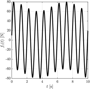
(a) Time-domain signal $f_{1}(t)$

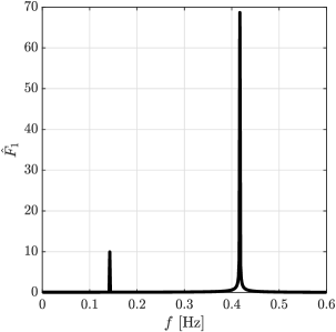
(c) Frequency-domain signal $\hat{F}_{1}(f)$

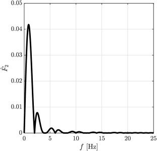
(d) Frequency-domain signal $\hat{F}_{2}(f)$

Figure 1: Excitation signal in the time and frequency domain—SDOF system.

An advantage of studying simple SDOF systems is that it is possible to derive analytical solutions in closed-form and consequently, a suitable error measure is easily defined. In the following, the error in displacements based on the $L_{2}$-norm ($\epsilon_{L_{2}}$) is used to assess the accuracy of the time integration algorithms

$$\epsilon_{L_{2}}=\cfrac{\int\limits_{t=0s}^{t_{\mathrm{sim}}}(u_{\mathrm{ref}}(t)-u_{\mathrm{num}}(t))^{2}\;\mathrm{d}t}{\int\limits_{t=0s}^{t_{\mathrm{sim}}}u_{\mathrm{ref}}(t)^{2}\;\mathrm{d}t}\times 100[\%]\,,$$ (4cy)

where $u_{\mathrm{ref}}(t)$ denotes the analytical (theoretical) solution and $u_{\mathrm{num}}(t)$ represents the numerical solution obtained utilizing a specific time-stepping algorithm.

At this point, let us recall the analytical solution for the free vibration response of undamped and damped SDOF systems [49]. In this particular case, no external excitation force is acting on the structure and therefore, the ICs determine the structural dynamic behavior. The solution to the second-order ODE—Eq. (4cm)—for $\zeta\,{=}\,0$ is

$$u(t)=u_{0}\cos(\omega_{\mathrm{n}}t)+\cfrac{\dot{u}_{0}}{\omega_{\mathrm{n}}}\,\sin(\omega_{\mathrm{n}}t)\,,$$ (4cz)

whereas in the damped case, i.e., $\zeta\neq 0$, the theoretical solution takes the following form

$$u(t)=\exp(-\zeta\omega_{\mathrm{n}}t)\left(u_{0}\cos(\omega_{\mathrm{D}}t)+\cfrac{\dot{u}_{0}+\zeta\omega_{\mathrm{D}}u_{0}}{\omega_{\mathrm{D}}}\,\sin(\omega_{\mathrm{D}}t)\right)\,,$$ (4da)

where $\omega_{\mathrm{D}}$ is the natural (angular) frequency of the damped systems, defined as $\omega_{\mathrm{D}}\,{=}\,\omega_{\mathrm{n}}\sqrt{1-\zeta^{2}}$. Considering an external excitation, the solution is a bit more complex since now not only the complementary (transient response) but also the particular part (steady-state response) of the solution have to be taken into account. The latter one is solely related to the non-homogeneous ODE and therefore, determined by the excitation function. The general solution for a harmonic excitation of an undamped system featuring both sine- and cosine-terms with two distinct frequencies is given in closed-form as

$$\begin{split}u(t)=&\left(u_{0}-\cfrac{\hat{f}_{1}}{k}\,\cfrac{1}{1-\left(\nicefrac{{\omega_{1}}}{{\omega_{\mathrm{n}}}}\right)^{2}}\right)\cos(\omega_{\mathrm{n}}t)+\left(\cfrac{\dot{u}_{0}}{\omega_{\mathrm{n}}}-\cfrac{\hat{f}_{2}}{k}\,\cfrac{\nicefrac{{\omega_{2}}}{{\omega_{\mathrm{n}}}}}{1-\left(\nicefrac{{\omega_{2}}}{{\omega_{\mathrm{n}}}}\right)^{2}}\right)\sin(\omega_{\mathrm{n}}t)+\\ &\left(\cfrac{\hat{f}_{1}}{k}\,\cfrac{1}{1-\left(\nicefrac{{\omega_{1}}}{{\omega_{\mathrm{n}}}}\right)^{2}}\right)\cos(\omega_{1}t)+\left(\cfrac{\hat{f}_{2}}{k}\,\cfrac{1}{1-\left(\nicefrac{{\omega_{2}}}{{\omega_{\mathrm{n}}}}\right)^{2}}\right)\sin(\omega_{2}t)\,.\end{split}$$ (4db)

In order to assess the accuracy of the proposed time integrator in relation to established methods, Newmark’s method [2] and Bathe’s method [12, 18] are included in the analysis. Both methods are second-order accurate, whereas Newmark’s method is a single-step scheme and Bathe’s method is a composite scheme consisting of two sub-steps. Due to the simplicity of the investigated systems, only the accuracy is considered, while the computational costs are essentially negligible.

The displacement error in the $L_{2}$-norm for the different set-ups of the SDOF system is plotted in Fig. 3.1. The thin dash-dotted lines are included to illustrate the theoretically optimal convergence behavior. We clearly observe that the proposed time-stepping method is converging with the optimal rate for all examples until the error reaches a plateau at roughly $1\times 10^{-9}\%$. Independent of the ICs, the presence of physical damping, or the external loading functions, high rates of convergence are achieved which highlights the superior performance of the novel method. The error plateau is clearly related to round-off errors that are inevitable in the numerical implementation of the algorithm.

(a) Case #1

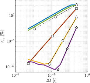
(b) Case #2

(c) Case #3

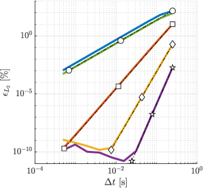
(d) Case #4

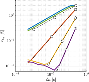
(e) Case #5

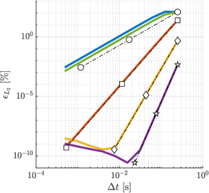
(f) Case #6

Figure 2: Displacement error in the $L_{2}$-norm for the different configurations of the single degree of freedom system. The dash-dotted lines indicate the optimal rates of convergence corresponding to slopes of 2 (circle), 4 (square), 6 (diamond), and 8 (pentagram), respectively.

As mentioned before, Bathe’s method is included in the comparison as a reference solution for a more recently developed algorithm. It is an unconditionally stable composite time integration scheme consisting of two sub-steps. In the first sub-step the constant average acceleration method is employed, while in the second on a three-point backward difference method is utilized. This combination yields a lower period elongation compared to Newmark’s method, while introducing a certain degree of numerical damping. More details on the performance of this method can be found in the pertinent literature [12, 14, 16, 19, 17, 18]. Bathe’s method has been intensively tested and is also implemented in the commercial finite element software ADINA. Based on the characteristics of Bathe’s method it is expected that it exhibits similar convergence properties compared to the present scheme of order $\mathcal{O}(1,1)$. Due to the use of two sub-steps, which in trun means that the computational effort is roughly doubled per time step, the overall error is slightly lower for Bathe’s method. Please keep in mind that for a fair comparison in terms of accuracy and computational effort, the time step should be doubled for Bathe’s time-stepping scheme.

3.2 Single degree of freedom system: Period elongation and amplitude error

The main goal of every time-stepping scheme is to achieve a high-quality approximation of the actual dynamic response of the structure that is being investigated. To this end, the time increment must selected such that the maximum frequency $f_{\mathrm{max}}$ of interest is well resolved. As a rule of thumb, it is often stated that ten increments per smallest period of interest $T_{\mathrm{min}}\,{=}\,\nicefrac{{1}}{{f_{\mathrm{max}}}}$ are sufficient to achieve reasonably accurate results [1]

$$\Delta t=\cfrac{T_{\mathrm{min}}}{10}\,.$$ (4dc)

However, considering problems where highly precise numerical solutions are required and the time integration method is only second-order accurate (which applies to most established methods such as Newmark’s method [2], the HHT-$\alpha$ method [3], the generalized-$\alpha$ method [23], Bathe’s method [12], etc.), this estimate of the time step size is generally not sufficient. From experience, approximately 100 sampling points per smallest period are recommended for high-fidelity simulations [51, 6].

The situation is obviously different when studying high-order accurate time-stepping methods such as the one proposed in this article. Here, larger time increments are possible due to the increased accuracy of the algorithm. Hence, it is in principle possible to apply similar refinement strategies in both space and time. The spatial h-refinement corresponds to a decrease in the time step size $\Delta t$ in the time domain, while an increase in the polynomial order of the shape functions is equivalent to an elevation of the order of the time integrator. Thus, to achieve a highly accurate solution with the least numerical costs a holistic hp-refinement strategy might be developed that is not only limited to the spatial discretization but also exploited for the temporal one. This, however, is out of the scope of the current contribution, where we want to introduce the algorithm and discuss its fundamental properties. Therefore, three important quantities, i.e., stability, amplitude error (AE), and period elongation (PE), will be briefly discussed in the remainder of this section. To this end, we consider the SDOF system described by case #1 for which the analytical solution is known: $u(t)\,{=}\,\cos(\omega_{\mathrm{n}}t)$. The simulation is run for 10,000 periods of vibration to study the effect of long-term numerical analysis. For a complete analysis, different IVPs with different ICs, damping, and loading functions would have to be considered. However, the defining numerical properties of the time integration scheme can be investigated by only solving the problem stated above [1]. For a general comparison, the results obtained using Newmark’s method (constant average acceleration), the HHT-$\alpha$ method ($\alpha\,{=}\,-0.05;$default setting in ABAQUS/standard), the generalized-$\alpha$ method ($\rho_{\infty}\,{=}\,0.8$), and Bathe’s method ($\gamma\,{=}\,(2-\sqrt{2})\Delta t$; splitting ratio) are included in the discussion.

3.2.1 Stability

In many problems of practical interest, the response of a structure is dominated by a limited range of frequencies, while the contribution of higher modes is essentially negligible. Hence, it is not meaningful to assign a time step size $\Delta t$ depending on the smallest period of the numerical system. Instead, we are only interested in the maximum frequency with a significant contribution to the structural response. This means, the higher modes are integrated with a time increment that not sufficient to fully resolve them. Hence, the question arises how the time-stepping scheme can handle large values of the ratio $\nicefrac{{\Delta t}}{{\tilde{T}_{\mathrm{min}}}}$, where $\tilde{T}_{\mathrm{min}}$ denotes the smallest (numerical) period of the system under investigation. This leads us to the topic of stability of a time-stepping scheme.

According to Ref. [48], Padé-based time integrators are unconditionally stable since the spectral radius of the rational approximation—see Eq. (4v)—of the matrix exponential—see Eq. (4u)—is of unit value, which means that amplitude decay is not observed in these methods. Unconditional stability is a very useful property to have as the error in the simulation of a dynamic problem will not diverge independent of the choice of the time step size $\Delta t$. Note that if the value for $\Delta t$ is chosen incorrectly, i.e., too large, the solution can still be arbitrarily wrong.

3.2.2 Amplitude error

Please note that a rigorous study of the amplification matrix for the proposed approach is out of the scope of the current contribution and will be included in future communications on a high-order implicit scheme with controllable numerical damping. Nonetheless, a simplified error measure referred to as amplitude error (AE) is introduced at this point to conclusively illustrate the performance of the novel time integrator. To this end, the amplitude of the displacement response is evaluated at multiplies of the actual period of vibration $T_{\mathrm{n}}\,{=}\,\nicefrac{{2\pi}}{{\omega_{\mathrm{n}}}}$ and a relative error is computed over all periods

$$\mathrm{AE}=\cfrac{1}{N}\sum\limits_{k=1}^{N}\cfrac{||u_{\mathrm{ref}}(kT_{\mathrm{n}})-u_{\mathrm{num}}(kT_{\mathrm{n}})||}{u_{\mathrm{ref}}(kT_{\mathrm{n}})}\times 100[\%]\,.$$ (4dd)

The results of this particular analysis are depicted in Figs. 3a and 3b in linear and logarithmic scale, respectively. The numerical results highlight that the novel scheme shows a very low amplitude error over time even if long-term simulations are investigated. It can be observed that depending on the chosen order already rather large time steps yield exceptionally accurate results in terms of the recovery of the amplitude of the displacement response. To put this into perspective, recall that in engineering analysis an error of roughly 1% is often deemed acceptable. Taking this measure, we see that the eighth-order accurate scheme provides accurate results already for a time step $\Delta t\,{=}\,\nicefrac{{T_{\mathrm{n}}}}{{2}}$, which is the absolute minimum increment that is required to theoretically resolve the vibration for low-order schemes. Naturally, smaller time steps are required considering lower approximation orders. Considering the sixth-order accurate algorithm a time step of $\Delta t\,{<}\,\nicefrac{{T_{\mathrm{n}}}}{{3}}$ is needed, while in the fourth-order case the time increment needs to be reduced further to $\Delta t\,{<}\,\nicefrac{{T_{\mathrm{n}}}}{{8}}$. Recall that established time integration methods are often only second-order accurate and therefore, a significantly smaller time step is required for those techniques. From Fig. 3b, we infer that $\Delta t\,{<}\,\nicefrac{{T_{\mathrm{n}}}}{{85}}$ is needed to achieve the prescribed error threshold of 1%. Thus, by increasing the order of accuracy of the time marching algorithm, the required time step can be significantly reduced. This behavior is expected and corresponds to what we observe when increasing the polynomial order of the spatial discretization. It has to be kept in mind, however, that by increasing the order of accuracy, we also increase the numerical costs of the method which will be discussed in more detail using more complex examples featuring a moderate number of DOFs.

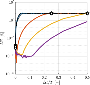
(a) Relative amplitude error in semi-log scale

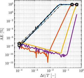
(b) Relative amplitude error in log-log scale

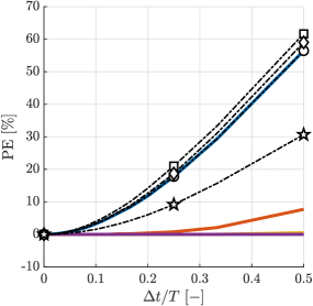
(c) Period elongation

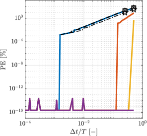
(d) Period elongation in log-log scale

Figure 3: Amplitude error and period elongation after 10,000 periods of vibration—Comparison of the novel scheme with established methods.

Since the amplitude error uses the displacement response evaluated at multiples of the natural period of the system under investigation it essentially combines two types of errors: (i) the actual error in the maximum displacement and (ii) the period elongation (PE) of the numerical algorithm. Consequently, we will have a closer look at the PE error in the following subsection.

3.2.3 Period elongation

The error cause by period elongation leads to the computational phenomenon referred to as numerical dispersion, i.e., the numerical solution seems to approximate a system with a different natural frequency. This shift can be both positive (as is the case for Newmark’s constant average acceleration method) or negative (as is the case in the central difference method). That is to say, in the numerical results either a shift to a higher or lower frequency will be apparent.

The error in the approximation of the natural period $T_{\mathrm{n}}$ is assessed by determining the peak values of the displacement response and saving the corresponding time values in a vector. Computing the differences between subsequent components of the time vector gives us the values for the natural period as approximated by the numerical solution.

$$\mathrm{PE}=\cfrac{1}{N}\sum\limits_{k=1}^{N}\cfrac{t\left(u_{\mathrm{max,num}}^{(k)}\right)-t\left(u_{\mathrm{max,ref}}^{(k)}\right)}{t\left(u_{\mathrm{max,ref}}^{(k)}\right)}\times 100[\%]\,,$$ (4de)

where $u_{\mathrm{max,num}}^{(k)}$ and $u_{\mathrm{max,ref}}^{(k)}$ are the maximum amplitude values for the k-th vibration. The value that is calculated here is an average period elongation over 10,000 vibration periods as mentioned before.

The numerical results of the PE analysis are depicted in Figs. 3c and 3d in linear and logarithmic scale, respectively. Due to the accuracy of the proposed time-stepping method, even after 10,000 periods of vibration there is basically no phase shift detectable and therefore, the error is set to the value of machine precision eps to evaluate the logarithm. In the initial stage, we observe a monotonous decrease of the PE-error before a sudden jump occurs, telling us that for the chosen simulation time no phase shift is present in the numerical results. Overall, the curves highlight that the proposed scheme exhibits very small values of PE or in other words, a negligible numerical dispersion is introduced. Thus, the present method is very attractive for long-term simulations with high accuracy requirements. We observe that the error in the natural period is basically negligible over the entire range of time increments if a method of order six or eight is chosen. Even at order four the shift in frequency is significantly lower compared to all established second-order accurate methods. For the maximum time step $\Delta t\,{=}\,\nicefrac{{T_{\mathrm{n}}}}{{2}}$, the proposed algorithm exhibits PE-values of approximately 0%, 0.5%, 7.7%, and 56.5%. In terms of the PE-error, the worst performance is exhibited by the HHT-$\alpha$ method with 61.7%, while Bathe’s method shows the best performance for all second-order approaches with 30.7%.

In summary, the numerical results demonstrate that any time-stepping method can be used and is very accurate as long as the ratio of time step to natural period (or period of interest) $\nicefrac{{\Delta t}}{{T_{\mathrm{n}}}}$ is below 0.01. In cases where this ratio is larger, the investigated methods show distinct difference that need to be taken into account when solving dynamical problems.

3.3 Dynamic behavior of a rectangular domain

In this section, the dynamic behavior of a two-dimensional rectangular body in plane stress conditions is considered [52]. In principle, the structure acts as a one-dimensional rod with the following material properties: Young’s modulus $E\,{=}\,100\,$Pa, Poisson’s ratio $\nu\,{=}\,0.0$, and mass density $\rho\,{=}\,1\,$kg/m³. The dimensions of the rectangular domain are $L\,{=}\,1\,$m and $h\,{=}\,0.2\,$m (see Fig. 4). A pressure load is applied at the right edge of the rod, while displacements in horizontal direction are fixed at its left edge. In contrast to the examples reported in the body of literature [33, 17, 4], the loading is not applied as a Heaviside function, even though an analytical solution is readily available due to the (mathematical) simplicity of the excitation. Instead, a time-dependent amplitude function $p(t)$ in form of a sine-burst is used

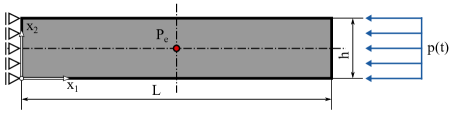
Figure 4: Homogeneous rectangular rod under plane stress conditions.

$$p(t)=P_{0}\sin(2\pi f_{\mathrm{ex}}t)\exp^{-\cfrac{1}{2}\left(\cfrac{t-t_{0}}{\tau}\right)^{2}}\,,$$ (4df)

where $f_{\mathrm{ex}}$ is the center frequency of the excitation signal, $P_{0}$ is the amplitude, and for the sake of simplicity, the variables $\tau$ and $t_{0}$ are chosen as functions of the period of excitation $T\,{=}\,\nicefrac{{1}}{{f_{\mathrm{ex}}}}$ as

$$\tau=T\qquad\text{and}\qquad t_{0}=4T\,.$$

Hence, the excitation signal is defined by a single parameter which is $f_{\mathrm{ex}}$. Note that the chosen excitation function makes the derivation of a analytical solution based on Duhamel’s integral very difficult and therefore, the reference results for this example are based on a numerical overkill solution of the system. An analytical solution for the displacement response due to a trigonometric excitation functions can be found in Ref. [53], while the solution for a Heaviside excitation are provided in Ref. [52].

In Fig. 5, both the time history and the frequency spectrum of the loading function are depicted. For the current analysis, the center frequency $f_{\mathrm{ex}}$ is set to $50\,$Hz, while the amplitude of the loading function $P_{0}$ is taken as $1\,$N. The maximum frequency of interest $f_{\mathrm{max}}$ is determined at the threshold when the amplitude in the frequency-spectrum is constantly below 1% of its maximum value. In our specific example, $f_{\mathrm{max}}$ is 74.125 Hz. To obtain a reasonable temporal resolution it is recommended (at least for commonly used second-order accurate time-stepping schemes) to employ at least 20 time steps per period of vibration determined by the maximum frequency of interest. Thus, an upper limit for the time step size would typically be $\Delta t_{\mathrm{max}}\,{=}\,\nicefrac{{1}}{{(20f_{\mathrm{max}})}}\,{=}\,6.75\times 10^{-4}\,$s. However, due to the use of a high-order time-stepping scheme the maximum time increment can be significantly increased to $\Delta t_{\mathrm{max}}\,{=}\,1.0\times 10^{-2}\,$s.

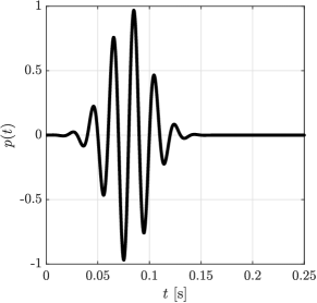
(a) Time-domain signal $f(t)$

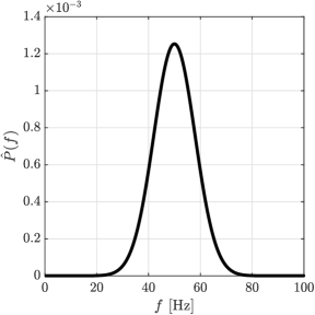
(b) Frequency-domain signal $\hat{F}(f)$

Figure 5: Excitation signal in the time and frequency domain—Rod.

In the current contribution, the main goal is to study the performance (accuracy and efficiency) of the proposed time integration scheme. At this point, we are not interested in including effects due to the spatial discretization in our analysis. Therefore, we limit our discussions on meshes consisting of bi-linear (4-node) finite elements. These, elements are implemented in virtually every commercial finite element code and are widely used in structural dynamics. We are well aware of the fact that, in general, high-order finite elements offer advantages in terms of higher convergence rates [54] and if they are based on Lagrangian shape functions and non-equidistant nodal distributions (e.g., the spectral element method (SEM) [55, 56]) the mass matrix can easily be diagonalized [6]. However, they have only found limited application outside academia and therefore, our analysis is at least for now restricted to elements with linear shape functions.

It is well-known that a high-order accurate time integration scheme is numerically more expensive on a per time step basis compared to low-order schemes and therefore, the higher costs need to be amortized by more accurate solutions and consequently, the possibility to use significantly larger time steps. Overall, a solution with a prescribed error threshold needs to be achieved with the least possible computational effort. In this section, all analyses are compared with the constant average acceleration method of the Newmark family [2]. This established time-stepping scheme serves as a benchmark for assessing the quality of the numerical solution in terms of accuracy and the computational costs.

Considering the spatial discretization eight different meshes consisting of square-shaped (bi-linear) finite elements have been set up. In the coarsest mesh, the element size has been set to $0.1\,$m, i.e., 20 elements (10$\times$2) are created. For each new discretization, the element size is halved and thus, the number of elements is increased by a factor of four. For the finest mesh, we obtain 327,680 elements (1,280$\times$256). That is to say, in terms of the number of degrees of freedom ($n_{\mathrm{DOF}}$), we cover a range from 66 to 658,434 DOFs, giving us a good insight into the performance of the present time integrator for small to medium-sized systems. Note that in the current implementation a direct solver is used in each time step, i.e., in linear dynamics the decomposition of the system matrix is pre-computed such that only forward and backward substitution steps need to be performed. For even larger systems, it is worth exchanging the direct solver with an iterative solver to facilitate a parallel implementation of the time-integrator on high-performance clusters [57].

Because the Poisson’s ratio is set to zero and therefore, the structure essentially behaves like a one-dimensional rod, the longitudinal (pressure) wave velocity, denoted as $c_{\mathrm{L}}$ is simply defined as

$$c_{\mathrm{L}}=\sqrt{\cfrac{E}{\rho}}\,.$$ (4dg)

We have to keep in mind, however, that this expression for the wave velocity only holds for a one-dimensional structure. According to Eq. (4dg), the wave velocity is $10\,\nicefrac{{\mathrm{m}}}{{\mathrm{s}}}$ in our example. The corresponding wavelength $\lambda$ is related to the frequency and the wave velocity by

$$\lambda=\cfrac{c_{\mathrm{L}}}{f_{\mathrm{ex}}}\,.$$ (4dh)

For the given values, the wavelength is $\lambda\,{=}\,0.2\,$m. Consequently, the spatial resolution of the wave packets varies between 2 and 256 elements per wavelength. As a rule of thumb, 10 elements with linear shape functions are always recommended although it has been shown in Ref. [54] that this is an absolute minimum, and the error is still well above the 1% threshold.

For each simulation, the so-called Courant-Friedrichs-Lewy (CFL) number can be determined, which provides a necessary condition for the convergence of a numerical solution to partial differential equations (PDEs) [58]. Although, it is closely related to the numerical analysis of explicit time integration schemes, we would like to mention it as a useful measure to assess the interplay between spatial and temporal discretizations. It is commonly defined as

$$\mathrm{CFL}=\cfrac{c\,\Delta t}{\Delta x}$$ (4di)

where $c$ is the characteristic wave velocity of the medium and $\Delta x$ denotes the element size (in a structured grid). Hence, the value of the CFL-number tells us through how many elements a wave can travel per each time step. This definition is, however, related to finite elements featuring linear shape functions. In general, a CFL-number below the value of one means that a wave travels less than the distance between two neighboring nodes.

3.3.1 Analysis of the computational costs

As mentioned before, it is only natural that high-order accurate time integration schemes are invariably more costly per time step compared to conventionally used second-order schemes. Therefore, it is worthwhile to investigate the required computational time. In the following, we will normalize the computational times obtained with the present high-order scheme with respect to the values obtained employing Newmark’s constant average acceleration method. The results of this analysis are depicted in Fig. 6. The simulations are run for the eight different discretizations with a time step size of $\Delta t\,{=}\,1.5625\times 10^{-4}\,$s, which results in 6,400 time steps for a simulation time of $t_{\mathrm{sim}}\,{=}\,1\,$s.

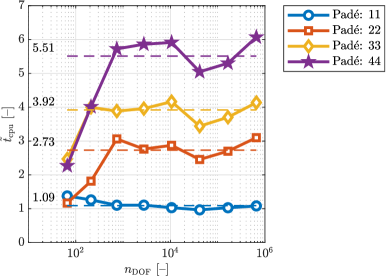
Figure 6: Computational time normalized with respect to Newmark’s constant average acceleration method—Rod.

As derived in Sect. 2.4.1, the present scheme of order $\mathcal{O}(1,1)$ is mathematically identical to Newmark’s constant average acceleration method and therefore, the computational times of both approaches should be (ideally) identical. In Fig. 6, we observe that a median value of 1.09 is reached for the normalized computational time $\tilde{t}_{\mathrm{cpu}}$ over a wide range of number of DOFs. This slight difference from the theoretically expected value of 1.0 is related to the different implementations regarding the solution procedure introduced in Sect. 2, compared to standard implementations of Newmark’s method as detailed in Ref. [1]. Overall, this is of no concern and shows again the good agreement. Considering the present time integration method of orders $\mathcal{O}(2,2)$, $\mathcal{O}(3,3)$, and $\mathcal{O}(4,4)$ which are fourth-, sixth-, and eighths-order accurate, respectively, an increase in the computational costs is noted. This increase is, however, very moderate, and median values of 2.73, 3.92, and 5.51 are achieved for the different schemes. That is to say, for this particular example the eighth-order accurate scheme is less than six times more costly than a standard second-order accurate implicit method of the Newmark family. This value is very promising considering the gained accuracy.

3.3.2 Analysis of the accuracy of the time-integrator

Besides the computational costs, the attainable accuracy is another important aspect when investigation time-stepping methods. Here, the convergence with respect to the exact solution of the discretized problem is studied. We are only interested in assessing the error introduced by the temporal discretization and neglect additional sources of errors such as the spatial discretization and incorrect mathematical assumptions on the material behavior.

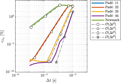
Figure 7: Displacement error in the $L_{2}$-norm for the homogeneous rectangular rod. The dash-dotted lines indicate the optimal rates of convergence corresponding to slopes of 2 (circle), 4 (square), 6 (diamond), and 8 (pentagram), respectively.

In order to assess the accuracy the displacement error in the $L_{2}$-norm ($\epsilon_{L_{2}}$)—see Eq. (4cy)—is computed. In Fig. 7, the error is depicted for a spatial discretization using 1,280 (bi-linear) finite elements (80$\times$16). The convergence curves are virtually identical for the other discretizations and therefore, only this example is plotted. Similar to the simple SDOF-systems, we observe optimal convergence until an error plateau is reached. As theoretically predicted, the present integrator of order $\mathcal{O}(1,1)$ and Newmark’s constant average acceleration method yield identical results. Due to the higher rates of convergence a similar accuracy can be easily reached using much larger time step sizes when the novel approach is employed. Considering an error threshold of roughly 1%, which is acceptable in most engineering applications, a time increment of $\Delta t\,{=}\,8.4\times 10^{-5}\,$s is required for Newmark’s constant average acceleration method, while for the high-order schemes significantly larger values are acceptable. Considering the present scheme of order $\mathcal{O}(2,2)$, $\Delta t\,{=}\,1.4\times 10^{-3}\,$s is sufficient, while the time increment can be further increased for orders $\mathcal{O}(3,3)$ and $\mathcal{O}(4,4)$ to $\Delta t\,{=}\,4.1\times 10^{-3}\,$s and $\Delta t\,{=}\,7.6\times 10^{-3}\,$s, respectively. That is to say, the time step size can be increased by factors of 17, 49, and 90 for the novel time-integrator. The results discussed in the current subsection need to be combined with the findings of the previous subsection to arrive at a first conclusion regarding the viability of our high-order time-stepping method. To this end, we recall that the increased computational costs per time step are depicted in Fig. 6. Here, it has been observed that the costs increase by a factor of less than 3, 4, and 6 for the fourth-, sixth- and eighth-order accurate schemes. This is much lower compared the amount of time steps that can be saved. For this example, a speed-up of roughly 6, 12, and 15 can be achieved. However, note that this value is problem dependent and might also be related to the properties of the numerical method that is employed for the spatial discretization.

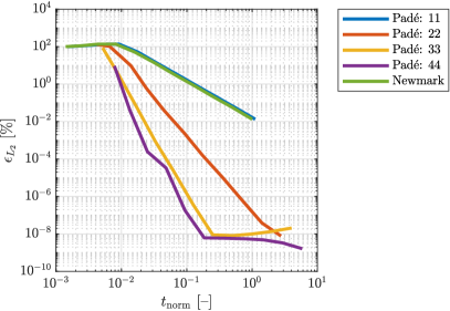
Figure 8: Displacement error in the $L_{2}$-norm for the different configurations over the normalized computational time—Rod.

The findings obtained in this section are summarized in Fig. 8, where we plot the attainable accuracy over the normalized computational time for a spatial discretization of 1,280 (bi-linear) finite elements (80$\times$16). Here, the simulation time is divided by the maximum value for Newmark’s constant average acceleration method, i.e., we take the computational time corresponding to Newmark’s method with a time step size of $\Delta t_{\mathrm{max}}\,{=}\,9.765625\times 10^{-6}\,$s as a reference. This figure is in principle a combination of Figs. 6 and 7, illustrating again the advantages of employing a high-order time integration scheme. We clearly observe that for a given simulation time the accuracy significantly increases when using the proposed method (add a vertical line to the graph with the targeted simulation time), while a prescribed error threshold can be reached in a shorter time (add a horizontal line to the graph with the targeted error value). Note that achieving this kind of efficiency is not trivial for high-order schemes, which are often too costly for moderately large systems. The results reported in this section for the relatively coarse mesh are also valid for the finer meshes that have been investigated for this example. Since the results are virtually identical it is not meaningful to provide all results and therefore, only selected graphs are included in the article.

For the sake of completeness, we include the displacement response in $x$-direction at point $P_{\mathrm{e}}$ located at (0.5 m, 0.1 m), see Fig. 9. The multiple reflections at the left and right edges are clearly seen, showing how the waves travels back and forth in the rod-like structure.

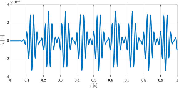
Figure 9: Displacement in $x$-direction at the observation point $P_{\mathrm{e}}$—Rod.

3.4 Lamb’s problems

In this section, we consider Lamb’s problem, in which wave propagation in a semi-infinite elastic domain are considered under plane strain conditions. The problem set-up and the material properties, reported in the following, are taken from Refs. [59, 15]. The geometry and loading conditions are depicted in Fig. 10. The material properties are chosen such that the P-wave velocity ($c_{\mathrm{L}}$) is 3,200 m/s, the S-wave velocity ($c_{\mathrm{T}}$) is 1,847.5 m/s, and the Rayleigh wave velocity ($c_{\mathrm{R}}$) is 1,671 m/s, while the mass density ($\rho$) is 2,200 kg/m³. The dimension of the computational domain $L$ is set to 3,200 m which ensures that no unwanted reflections from the boundaries of the structure are present in the displacement response ($t_{\mathrm{sim}}\,{=}\,1\,$s).

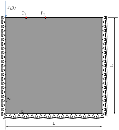
Figure 10: “Semi-infinite” elastic domain under plane strain conditions.

Based on the wave velocities and the mass density, Lamé’s constants $\tilde{\lambda}$ and $\tilde{\mu}$ (shear modulus) can be determined

$$c_{\mathrm{L}} =\sqrt{\cfrac{\tilde{\lambda}+\tilde{\mu}}{\rho}}\qquad \longrightarrow\qquad\tilde{\lambda} =c_{\mathrm{L}}^{2}\rho-\tilde{\mu}\,,$$ (4dj)

$$c_{\mathrm{T}} =\sqrt{\cfrac{\tilde{\mu}}{\rho}}\qquad \longrightarrow\qquad\tilde{\mu} =c_{\mathrm{T}}^{2}\rho\,.$$ (4dk)

To obtain the typical engineering constants Young’s modulus $E$ and Poisson’s ratio $\nu$ the following conversion is required

$$E =\cfrac{\tilde{\mu}(3\tilde{\lambda}+2\tilde{\mu})}{\tilde{\lambda}+\tilde{\mu}}\,,$$ (4dl)

$$\nu =\cfrac{\tilde{\lambda}}{2(\tilde{\lambda}+\tilde{\mu})}\,.$$ (4dm)

Accordingly, the Young’s modulus is 20 GPa and Poisson’s ratio is 0.33. These values can now be used to set up the numerical model for the wave propagation analysis.

The wave packets are excited by means of a concentrated point load located at the upper-left corner of the domain. The time-dependent excitation follows a Ricker wavelet function

$$F_{\mathrm{R}}(t)=F_{0}\left(1-\Psi(t)\right)\exp^{-\nicefrac{{1}}{{2}}\Psi(t)}\qquad\text{with}\qquad\Psi(t)=2\left(\pi f_{\mathrm{ex}}(t-t_{0})\right)^{2}\,,$$ (4dn)

where $f_{\mathrm{ex}}$ is the center frequency of the excitation, $F_{0}$ is the prescribed amplitude, and $t_{0}$ is a time parameter. In this example, the following values are chosen: $f_{\mathrm{ex}}\,{=}\,12.5\,$Hz, $F_{0}\,{=}\,100\,$N, and $t_{0}\,{=}\,\nicefrac{{2}}{{f_{\mathrm{ex}}}}$ and the time- as well as frequency-domain signal are depicted in Fig. 11. The maximum frequency of interest $f_{\mathrm{max}}$ is determined at the threshold when the amplitude in the frequency-spectrum is constantly below 1% of its maximum value. In our specific example, $f_{\mathrm{max}}$ is 34.54 Hz and therefore, a suitable time steps size to start the investigation is $\Delta t_{\mathrm{max}}\,{=}\,\nicefrac{{1}}{{2f_{\mathrm{max}}}}\,{\approx}\,1.5\times 10^{-2}\,$s.

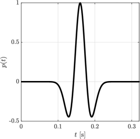
(a) Time-domain signal $f(t)$

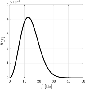
(b) Frequency-domain signal $\hat{F}(f)$

Figure 11: Excitation signal in the time and frequency domain—Lamb’s problem.

The Dirichlet boundary conditions are chosen according to Refs. [59, 15], i.e., the bottom and right edges of the domain are fixed (clamped), while symmetry boundary conditions are applied to the left edge. The top edge is assumed to be free and therefore, no additional Dirichlet or non-homogeneous Neumann boundary conditions are applied.

Considering the spatial discretization, we use bi-linear (4-node) quadrilateral elements, and the element size is selected as 5 m. Thus, 409,600 elements are created which corresponds to 821,762 DOFs. The spatial discretization is set up with respect to the Rayleigh wavelength being the wave type with the lowest wave velocity. According to Eq. (4dh), this also means that its wavelength is the smallest, making it the one defining the element size. For a maximum considered frequency of $f_{\mathrm{max}}\,{=}\,34.54\,$Hz, we get $\lambda_{\mathrm{R}}\,{=}\,48.38\,$m and thus, roughly ten elements per wavelength are employed. As mentioned before and shown in Ref. [54], this is an absolute minimum and would result in an error of above 1%. However, at this point, we are not interested in obtaining highly accurate results with a minimal error due to the spatial discretization, but we want to determine the error contributed by the temporal discretization and the chosen time-integrator. Therefore, the spatial resolution is sufficient for our purposes.

The displacement response due to the excitation by means of the point force following a Ricker wavelet are evaluated at two observation points $P_{1}$ and $P_{2}$ located at the top surface 640 m and 1280 m away from the excitation source. Contour plots of the entire domain for selected time instance, where we clearly observe the different wave types propagating through the structure are provided in Fig. 3.4, while the displacement histories for the two observation points are given in Fig. 13.

(a) $t\,{=}\,0.2508\,$s

(c) $t\,{=}\,0.4514\,$s

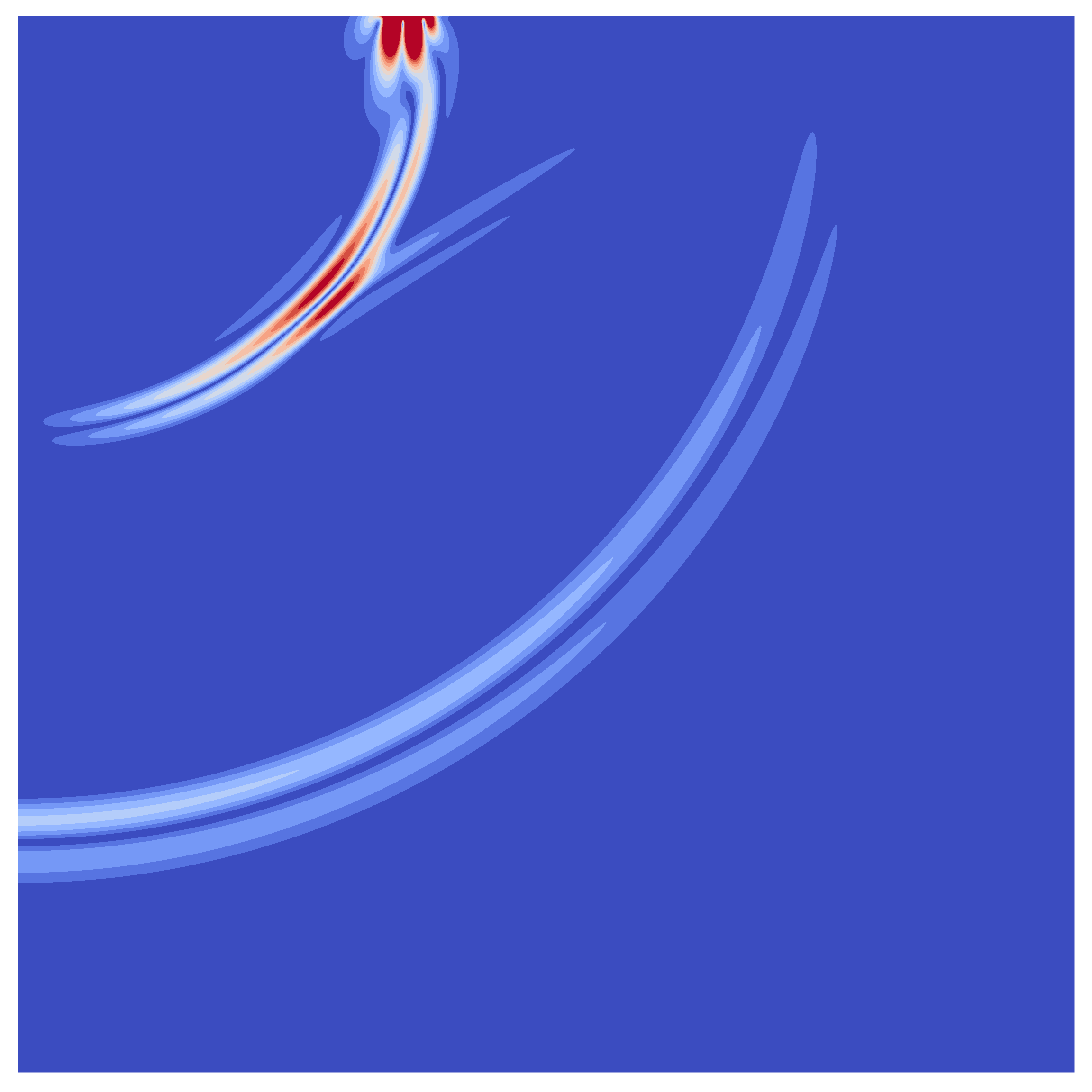
(d) $t\,{=}\,0.7523\,$s

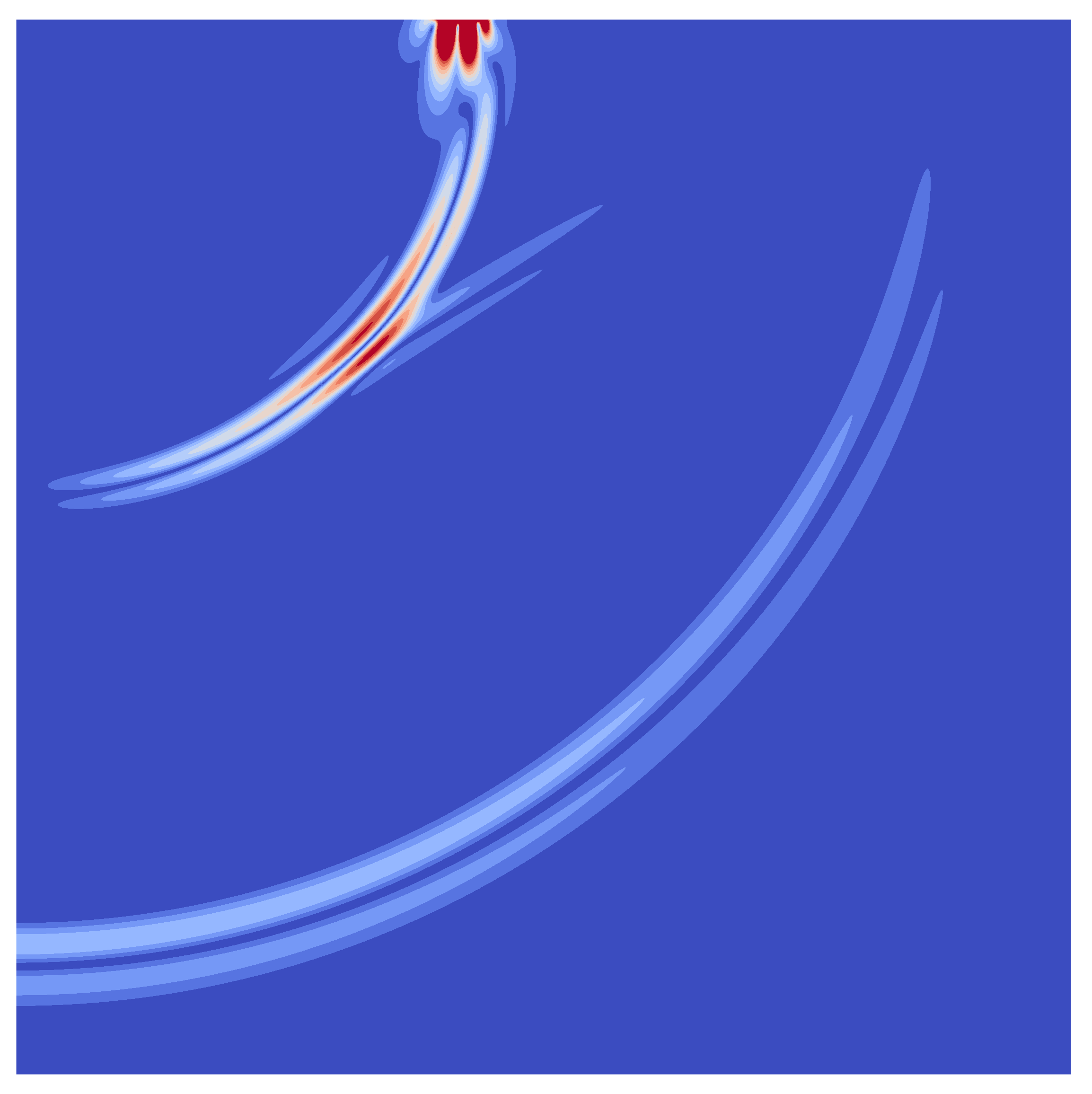
(e) $t\,{=}\,0.8527\,$s

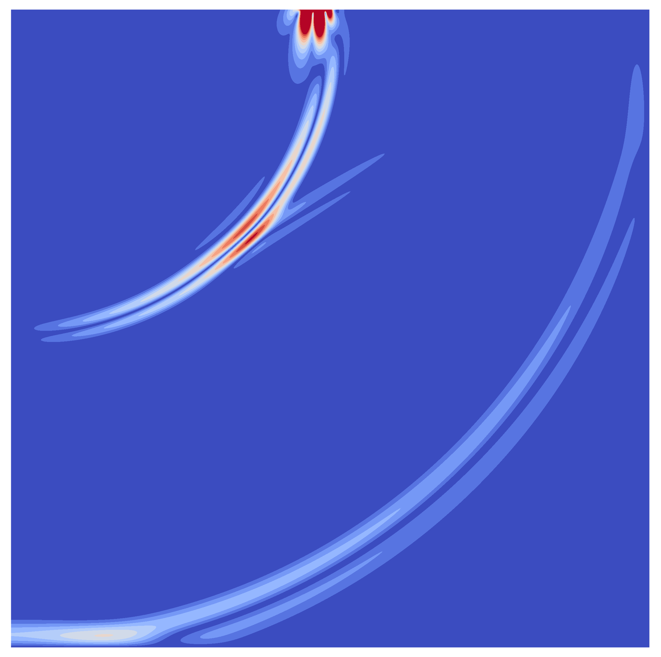
(f) $t\,{=}\,0.9530\,$s

Figure 12: Displacement field ($u_{\mathrm{mag}}$) for Lamb’s problem at different time instances ($\Delta t\,{=}\,2.34375\times 10^{-4}\,$s; Present scheme of order $\mathcal{O}$(4,4). In order to observe not only the dominant Rayleigh wave the maximum color value of the displacement is set to $1\times 10^{-5}\,$m.

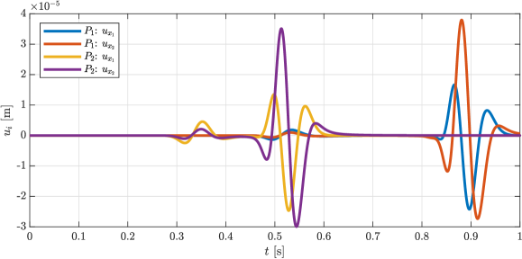
Figure 13: Displacement response at the observation points $P_{1}$ and $P_{2}$—Lamb’s problem.

3.4.1 Analysis of the computational costs

Lamb’s problem is only investigated for the spatial discretization discussed in the previous subsection, i.e., an element size of 5 m is selected leading to 821,762 DOFs. Utilizing a coarser discretization would lead to physically not meaningful results and is therefore, not conducted. On the other hand, a finer resolution would yield quickly several million DOFs, which is not feasible for the performance assessment done in this paper. For studying much larger systems, it is worth switching from a direct solver to an iterative solver which is out of the scope of this contribution but is a part of ongoing research activities. For this example, the normalized computational time with respect to Newmark’s constant average acceleration method is 1 for the present scheme of order $\mathcal{O}(1,1)$ (which is mathematically identical), 4.55 for order $\mathcal{O}(2,2)$, 5.53 for order $\mathcal{O}(3,3)$, and 9.96 for order $\mathcal{O}(4,4)$. These values are moderately higher compared to the ones obtained in Sect. 3.3.1. Still, we have to bear in mind that a significant increase in accuracy is achieved with elevating the order of the time-stepping scheme. It is obvious that the numerical overhead of a high-order technique is dependent on the selected equation solvers and the numerical model, i.e., sparsity and bandwidth of the matrix, among others. These factors will be thoroughly investigated in forthcoming communications.

3.4.2 Analysis of the accuracy of the time-integrator

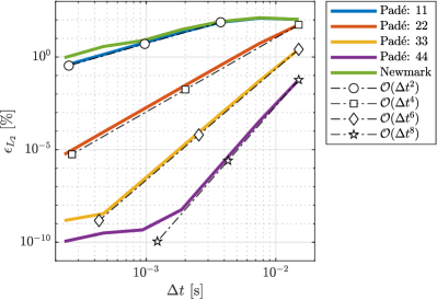
Figure 14: Displacement error in the $L_{2}$-norm for Lamb’s problem. The dash-dotted lines indicate the optimal rates of convergence corresponding to slopes of 2 (circle), 4 (square), 6 (diamond), and 8 (pentagram), respectively.

In order to assess the accuracy the displacement error in the $L_{2}$-norm ($\epsilon_{L_{2}}$)—see Eq. (4cy)—is computed. In Fig. 14, the error is depicted for the chosen spatial discretization. Similar to the previous numerical examples, we observe optimal convergence until an error plateau is reached. As theoretically predicted, the novel time integrator of order $\mathcal{O}(1,1)$ and Newmark’s constant average acceleration method yield identical results. Due to the higher rates of convergence a similar accuracy can be easily reached using much larger time step sizes when the novel approach is employed. Considering an error threshold of roughly 1%, which is acceptable in most engineering applications, a time increment of $\Delta t\,{=}\,4.01\times 10^{-4}\,$s is required for Newmark’s constant average acceleration method, while for the high-order schemes significantly larger values are acceptable. Considering the proposed time integrator of order $\mathcal{O}(2,2)$, $\Delta t\,{=}\,4.87\times 10^{-3}\,$s is sufficient, while the time increment can be further increased for orders $\mathcal{O}(3,3)$ and $\mathcal{O}(4,4)$ to $\Delta t\,{=}\,1.27\times 10^{-2}\,$s and $\Delta t\,{=}\,2.0\times 10^{-2}\,$s, respectively. That is to say, the time step size can be increased by factors of 12.14, 31.67, and 49.88 for the novel time-integrator. These values need to be put into perspective with the increased costs per times step as found in the previous subsection. There, it was observed that the computational effort increases by a factor of roughly 4.5, 5.5, and 10 for the fourth-, sixth- and eighth-order accurate schemes. Therefore, the attainable speed-up is observed to be 2.67, 5.73, and 5.01. Again, please keep in mind that this value is problem dependent and might also be related to the properties of the numerical method that is employed for the spatial discretization.

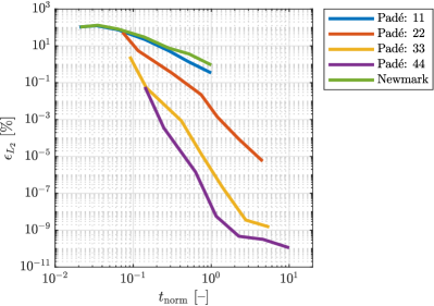
Figure 15: Displacement error in the $L_{2}$-norm for the different configurations over the normalized computational time—Lamb’s problem.

The conclusions that can be drawn from the findings reported in the current section are summarized in Fig. 15. Here, the attainable accuracy is plotted against the normalized computational time. As a reference, the computational time corresponding to Newmark’s method with a time step size of $\Delta t_{\mathrm{max}}\,{=}\,2.34375\times 10^{-4}\,$s is taken. The results again illustrate that employing a high-order time integration scheme leads to significant savings in terms of computational time for a prescribed error threshold or to significantly more accurate results for the same computational time.

3.5 Wave propagation in a mountainous region

As a final example, a three-dimensional mountainous region is chosen. Here, we are simulating the wave propagation in a mountainous region of size 6.94 km$\times$7.8 km to showcase the performance of the proposed time integration scheme for fully three-dimensional models. The initial STL file of the region is obtained using the online service Terrain2STL at http://jthatch.com/Terrain2STL/. The material properties are assumed as: Young’s modulus $E\,{=}\,55\,$GPa, Poisson’s ratio $\nu\,{=}\,0.2$, and the mass density $\rho\,{=}\,2400\,$kg/m³. Thus, the P-wave and S-wave velocities are $c_{\mathrm{L}}\,{=}\,5046\,$m/s and $c_{\mathrm{T}}\,{=}\,3090\,$m/s, respectively. In terms of boundary conditions, it is assumed that the displacements normal to the side and bottom faces are fixed. The excitation is realized by means of a concentrated force in $x_{2}$-direction applied at the centroid of the bottom surface. The excitation follows a Ricker wavelet with a center frequency of $f_{\mathrm{ex}}\,{=}\,2\,$Hz, while the time parameter is set to $t_{0}\,{=}\,\nicefrac{{1}}{{f_{\mathrm{ex}}}}$ (see Fig. 16 for the time- and frequency-domain signal). The maximum frequency of interest $f_{\mathrm{max}}$ is determined at the threshold when the amplitude in the frequency-spectrum is constantly below 1% of its maximum value. In our specific example, $f_{\mathrm{max}}$ is 5.53 Hz and therefore, a suitable time steps size to start the investigation is $\Delta t_{\mathrm{max}}\,{=}\,\nicefrac{{1}}{{2f_{\mathrm{max}}}}\,{\approx}\,9\times 10^{-2}\,$s.

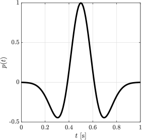
(a) Time-domain signal $f(t)$

(b) Frequency-domain signal $\hat{F}(f)$

Figure 16: Excitation signal in the time and frequency domain—Mountainous region.

The displacement response has been saved at the peak of the mountainous region (3,224 m, 4,160 m, 3,952 m) and at other points with 75% (3.224 m, 4,160 m, 2,912 m), 50% (3.224 m, 4,160 m, 1,976 m), and 25% (3,224 m, 4,160 m, 0,936 m) of the height. Since a highly complex octree mesh has been used the nodes nearest to those locations have been picked. The original geometry of the region and its discretization are depicted in Fig. 3.5.

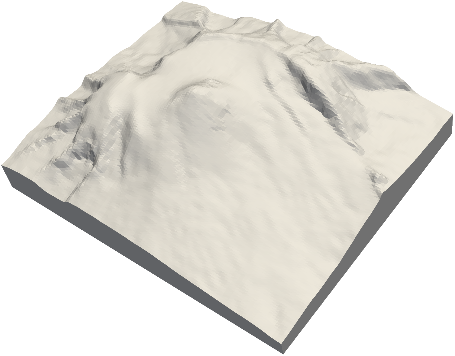
(a) STL data

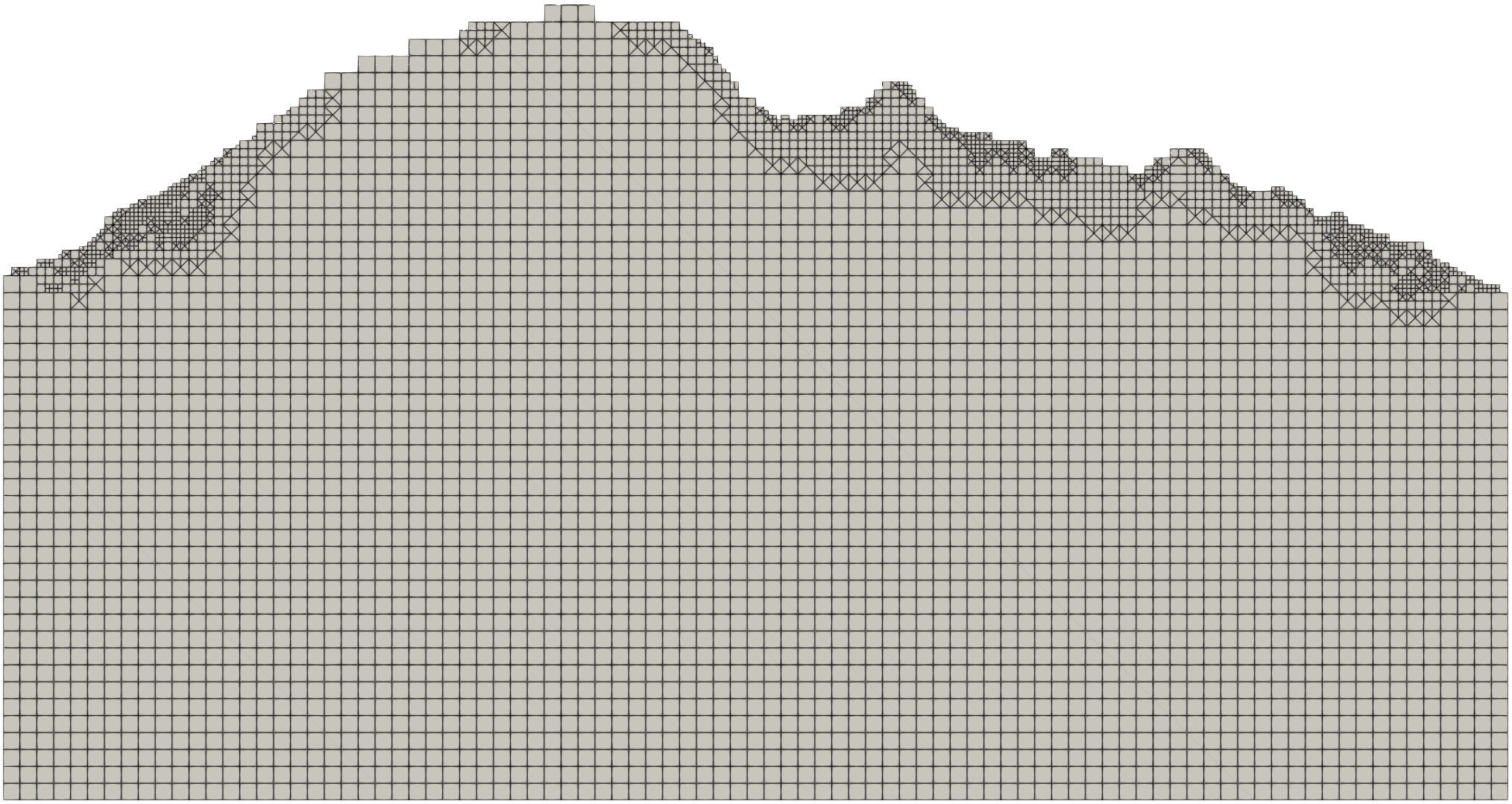
(c) Cut view of the discretization

Figure 17: Three-dimensional model of a mountainous region.

The simulations in this section are based the scaled boundary finite element method (SBFEM), which is a semi-analytical non-standard discretization technique. For a comprehensive introduction and thorough assessment of the performance of SBFEM, the interested reader is referred to the monograph by Song [60]. At this point, we only want to mention that using the SBFEM it is straightforward to set up octree meshes based on STL files without encountering the “hanging nodes” problem [61, 62]. Here, each element is modeled as a scaled boundary polyhedron and therefore, a conformal/compatible coupling between elements of different sizes is a priori guaranteed, i.e., there is no need for a special treatment as required in conventional FEA. In the current analysis, a simple octree mesh without trimming has been used for the sake of simplicity, but it is also possible to achieve geometry conforming meshes [63, 64] to improve the quality of the solution. Overall, the mesh consists of 173,786 octree cells (featuring linear shape functions on the boundary) with a ratio of 1/4 for the smallest (cell size: 26 m) to the largest cell (cell size: 104 m). Thus, we have 251,779 nodes in the discretization and consequently, 755,337 DOFs. In order to be able to obtain an accurate reference solution in a relatively short time, the central difference method in conjunction with a lumped (diagonal) mass matrix is applied. The time increment is set to $\Delta t_{\mathrm{CDM}}\,{=}\,1\times 10^{-4}\,$s. More details on the particular implementation of the CDM are discussed in Ref. [57].

In this three-dimensional example, we will compute the transient response using the novel time-stepping scheme of order $\mathcal{O}$(4,4) with the time step size $\Delta t_{\mathrm{max}}$. Additionally, simulations employing Newmark’s constant average acceleration method will be executed with time step sizes of $\Delta t_{\mathrm{max}}$ and $\nicefrac{{\Delta t_{\mathrm{max}}}}{{50}}$. Judging for the findings reported in the previous sections, a clear difference in the displacement history is expected for a time increment $\Delta t_{\mathrm{max}}$. However, when using the smaller time step size for Newmark’s method a significantly improved agreement is expected. Using this approach, we can gain some insights into the performance of the time integrator for complex three-dimensional problems. Extensive parametric studies for such examples are still computationally very expensive and prohibitive at this point. Snapshots of the wave propagation in the mountainous region for different time instances are depicted in Fig. 3.5. These contour plots illustrate the propagation of the primary wave through the mountainous region. In further, more sophisticated, analyses, numerical models of faults, different rock layers, and unbounded domains can be straightforwardly added.

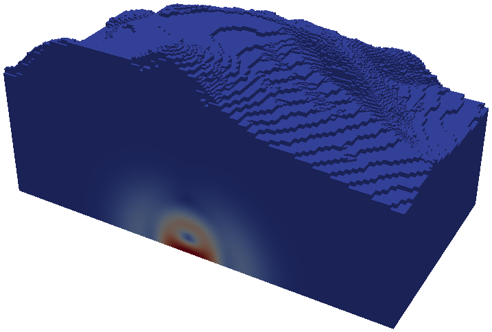
(a) $t\,{=}\,0.6058\,$s

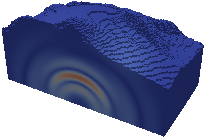
(c) $t\,{=}\,1.0097\,$s

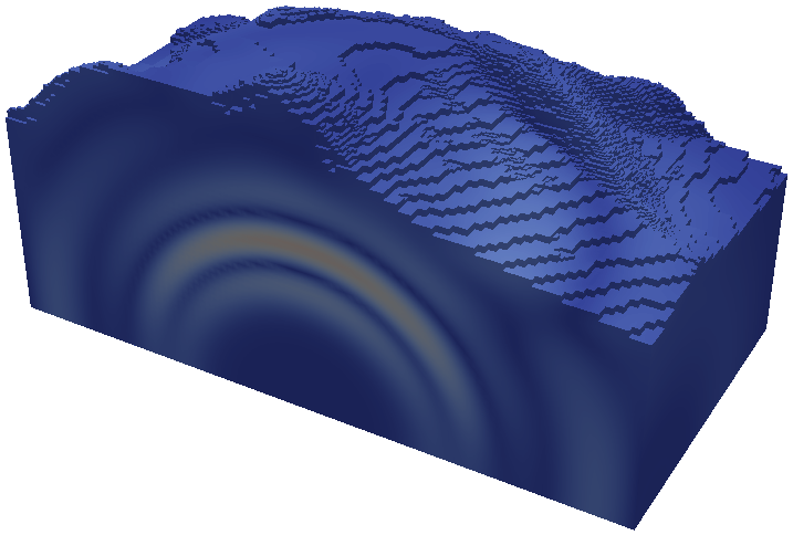
(d) $t\,{=}\,1.2117\,$s

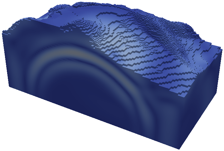
(e) $t\,{=}\,1.4136\,$s

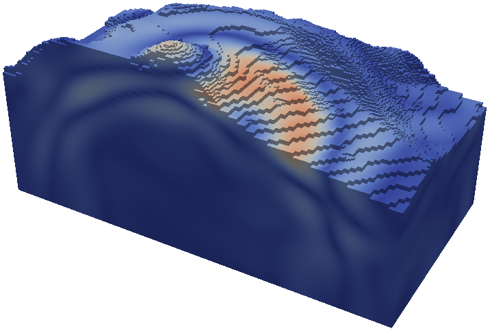
(f) $t\,{=}\,1.6156\,$s

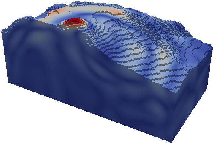
(g) $t\,{=}\,1.8175\,$s

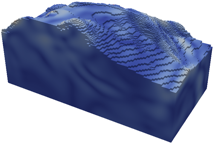
(h) $t\,{=}\,2.0194\,$s

Figure 18: Displacement field ($u_{\mathrm{mag}}$) for the mountainous region at different time instances ($\Delta t\,{=}\,0.0018\,$s; Padé scheme of order $\mathcal{O}$(1,1). For a better visibility of the propagating waves, the maximum color value of the displacement is set to $5\times 10^{-5}\,$m.

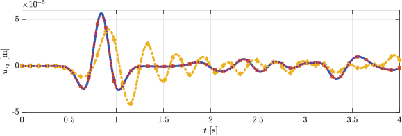
(a) Displacement response ($u_{\mathrm{{x_{2}}}}$) at point $P_{1}$(peak)

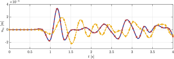
(b) Displacement response ($u_{\mathrm{{x_{2}}}}$) at point $P_{2}$(75% of the peak height)

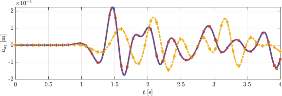
(c) Displacement response ($u_{\mathrm{{x_{2}}}}$) at point $P_{3}$(50% of the peak height)

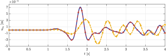
(d) Displacement response ($u_{\mathrm{{x_{2}}}}$) at point $P_{3}$(25% of the peak height)

Figure 19: Displacement history at the four observation points.

The displacement field $u_{x_{2}}$ at the four observation points is depicted in Fig. 3.5. Here, we observe clear differences in the response if the same time step size is used for both Newmark’s constant average acceleration method and the novel eighth-order scheme. The results obtained employing the proposed time-stepping scheme are very accurate and closely match the reference results. Since a very large time step has been chosen, we included markers to indicate the actual time points that have been computed. To obtain a smooth curve,we interpolated between these few points using $C_{1}$-contnuous cubic splines. Therefore, the small observed differences are not actually related to the time-integration itself but to the required interpolation. In contrast, if the time increment is significantly decreased for Newmark’s method (in this case by a factor of 50), also an excellent agreement of the results is noted compared to the reference solution. This result emphasizes again that highly accurate solution are obtained with the novel method for very large time step sizes. Considering the computational time, we normalize the values with respect to Newmark’s constant average acceleration method with the time increment $\Delta t_{\mathrm{max}}$. The novel eighth-order time-stepping algorithm only requires 4.05 times the computational time, while decreasing the time step size by a factor of 50 an increase in the consumed time by a 24.1 is observed. Note that for the current example, a large portion of the solution time is invested in the initial factorization of effective system matrices.

4 Conclusions and outlook on future research activities

In the present article, a high-order implicit time-stepping scheme based on a Padé series expansion of the matrix exponential function has been proposed. The salient features of this time integrator are: (i) accuracy of order $2p$, where $p$ is the polynomial degree of the diagonal Padé expansion; (ii) negligible period elongation for high-order schemes; (iii) no amplitude decay (no numerical damping); and (iv) high efficiency in the solution of the semi-discrete equations of motion. The proposed method is especially suited for applications where a high accuracy of the results is of utmost importance and long-term analyses are required. Although, it is generally argued that high-frequency numerical damping is a wanted property in time integrators, there are also applications where any damping (physical or numerical) is unwanted and would deteriorate the accuracy of the analysis. If, however, spurious waves are excited and damping is indispensable, preliminary results of the authors suggest that the addition of a very low amount of stiffness-proportional damping (i.e., $\beta_{\mathrm{R}}\,{<<}\,1$ and $\alpha_{\mathrm{R}}\,{=}\,0$) is adequate and might even out perform time-stepping methods offering high-frequency numerical damping. Note that the addition of damping does not impair the efficiency of the novel algorithm since a system of equations has to be solved in each time step anyway due to the implicit nature of the method.

In future research activities, the authors plan to extend the proposed scheme to include controllable numerical damping where the spectral radius of the amplification matrix is prescribed a priori. Thus, we will be able to construct a high-order family of time-stepping methods that offer A- and L-stable algorithms suitable for different areas of application. Additionally, to allow for large-scale transient analyses, the direct solver needs to be exchanged by a suitable iterative solver including tailored pre-conditioners. This also opens the pathway to a targeted parallelization of the algorithm and its use on high-performance applications.

Dedication

This paper is dedicated to the late Dr. John P. Wolf, who was a mentor and close friend to the first author of this paper, Chongmin Song. The presented research is highly influenced by the scientific contributions of Dr. John P. Wolf and Dr. Antonio Paranesso [43, 44] regarding the development of lumped-parameter models for dynamic soil-structure interaction analysis by means of Padé and partial fraction approximations. Therefore, the novel time integration scheme proposed in this article clearly benefits from the direct exposure to the guidance of Dr. John P. Wolf for which Chongmin Song is very grateful.

Appendix A Matrix exponential and Taylor series

For the sake of completeness and in the purpose of ensuring that the article is largely self-contained, we will repeat the necessary theory that is directly related to this paper. For more comprehensive information and a complete theory on matrix functions the interested reader is referred to the pertinent literature [65, 39].

The matrix exponential function of an arbitrary square matrix $\mathbf{A}$ can be defined using a Taylor series expansion

$$e^{\mathbf{A}}=\mathbf{I}+\sum\limits_{k=1}^{\infty}\cfrac{1}{k!}\mathbf{A}^{k}\,,$$ (4do)

where $\mathbf{I}$ is an identity matrix of the same dimensions as $\mathbf{A}$.

One important application of the matrix exponential function is to solve generic IVPs resulting in a system of linear ODEs written as

$$\mathbf{y}^{\prime}(x)=\mathbf{A}\mathbf{y}(x)$$ (4dp)

with the IC

$$\mathbf{y}(0)=\mathbf{y}_{0}\,.$$ (4dq)

The prime $\square^{\prime}$ denotes a derivative with respect to the argument of the function $x$. The general solution to this ODE is given by

$$\mathbf{y}(x)=e^{\mathbf{A}x}\mathbf{y}_{0}\,.$$ (4dr)

The matrix exponential $e^{\mathbf{A}x}$ is called the fundamental matrix of the system of ODEs expressed in Eq. (4dp). An important mathematical property of the function $e^{\mathbf{A}}$ is that it is commutative with respect to the matrix $\mathbf{A}$ and its inverse $\mathbf{A}^{-1}$, i.e.,

$$\mathbf{A}e^{\mathbf{A}}=e^{\mathbf{A}}\mathbf{A}\qquad\text{and}\qquad\mathbf{A}^{-1}e^{\mathbf{A}}=e^{\mathbf{A}}\mathbf{A}^{-1}$$ (4ds)

hold, which can be shown using the definition of the matrix exponential function given in Eq. (4do) by means of a Taylor series.

As a specific example, let us consider the case of free vibration of an undamped SDOF system. Equation (4cm) is written as

$$\ddot{u}+\omega_{n}^{2}u=0$$ (4dt)

with the initial conditions (see Eq. (2))

$$u(t=0)=u_{0}\quad\mathrm{and}\quad\dot{u}(t=0)=\dot{u}_{0}$$ (4du)

The matrix $\mathbf{A}$ in Eq. (4i) is defined as

$$\mathbf{A}=\begin{bmatrix}0&-\omega_{n}^{2}\\ +1&0\end{bmatrix}\,.$$ (4dv)

Here, $\mathbf{A}$ has two imaginary eigenvalues $\pm\mathrm{i}$. The matrix exponential function $e^{\mathbf{A}t}$ is expressed according to Eq. (4do) as a infinite sum of power functions

$$e^{\mathbf{A}t}=\begin{bmatrix}1&0\\ 0&1\end{bmatrix}+t\begin{bmatrix}0&-\omega_{n}^{2}\\ +1&0\end{bmatrix}+\dfrac{t^{2}}{2!}\begin{bmatrix}-\omega_{n}^{2}&0\\ 0&-\omega_{n}^{2}\end{bmatrix}+\dfrac{t^{3}}{3!}\ \begin{bmatrix}0&\omega_{n}^{4}\\ -\omega_{n}^{2}&0\end{bmatrix}+\dfrac{t^{4}}{4!}\begin{bmatrix}\omega_{n}^{4}&0\\ 0&\omega_{n}^{4}\end{bmatrix}+\cdots$$ (4dw)

This expression can be further simplified using the Taylor series expansions of the sine- and cosine-functions

$$\cos(x) =\sum\limits_{k=0}^{\infty}\dfrac{(-1)^{k}}{(2k)!}x^{2k} =1-\dfrac{x^{2}}{2!}+\dfrac{x^{4}}{4!}-\ldots$$ (4dxa)

$$\sin(x) =\sum\limits_{k=0}^{\infty}\dfrac{(-1)^{k}}{(2k+1)!}x^{2k+1} =x-\dfrac{x^{3}}{3!}+\dfrac{x^{5}}{5!}-\ldots$$ (4dxb)

Hence, the matrix exponential function in Eq. (4dw) can be given as

$$e^{\mathbf{A}t}=\begin{bmatrix}\cos(\omega_{n}t)&-\omega_{n}\sin(\omega_{n}t)\\ \dfrac{1}{\omega_{n}}\sin(\omega_{n}t)&\cos(\omega_{n}t)\end{bmatrix}\,.$$ (4dy)

Following Eq. (4dr), the solution of Eq. (4dt) with Eq. (4du) is obtained as

$$\left\{\begin{array}[]{c}\dot{u}\\ u\end{array}\right\}=\begin{bmatrix}\cos(\omega_{n}t)&-\omega_{n}\sin(\omega_{n}t)\\ \dfrac{1}{\omega_{n}}\sin(\omega_{n}t)&\cos(\omega_{n}t)\end{bmatrix}\left\{\begin{array}[]{c}\dot{u_{0}}\\ u_{0}\end{array}\right\}$$ (4ed)

which is consistent with the solution in Eq. (4db).

Appendix B Padé expansion of the exponential function

In a Padé expansion, a function is approximated as a ratio of two polynomials, i.e., a rational function. The Padé approximation of a function $y(x)$ of order $\mathcal{O}(L,M)$ is written as

$$y_{L/M}(x)=\cfrac{P_{L}(x)}{Q_{M}(x)}=\cfrac{p_{0}+p_{1}x+\ldots+p_{L}x^{L}}{q_{0}+q_{1}x+\ldots+q_{M}x^{M}}\,,$$ (4ee)

where $L$ and $M$ are the degrees of polynomials in the numerator and denominator, respectively. The constants $p_{k}$ ($k=0,1,\ldots,L)$ and $q_{k}$ ($k=0,1,\ldots,M)$ can be determined by equating the Padé series with a Taylor expansion. In the present study, only the diagonal Padé approximations of the exponential function $e^{x}$ is of interest. Hence, the order of the approximation is $\mathcal{O}(M,M)$ or in short $M$, which is expressed as

$$e_{M}^{x}=\cfrac{P_{M}(x)}{Q_{M}(x)}\,,$$ (4ef)

where the polynomials in the numerator and denominator are given by

$$P_{M}(x) =\sum\limits_{m=0}^{M}\cfrac{\left(2M-m\right)!}{m!\left(M-m\right)!}\;x^{m}\,,$$ (4ega)

$$Q_{M}(x) =P_{M}(-x)=\sum\limits_{m=0}^{M}\cfrac{\left(2M-m\right)!}{m!\left(M-m\right)!}\;(-x)^{m}\,.$$ (4egb)

From Eqs. (4eg), it is obvious that $Q_{M}(x)=P_{M}(-x)$ holds. The accuracy of the approximation is of the order of $2M$. The denominator polynomial $Q_{M}(x)$ of degree $M$ can be factorized as

$$Q_{M}(x)=\prod\limits_{i=1}^{M}\left(r_{i}-x\right)=\left(r_{1}-x\right)\left(r_{2}-x\right)\ldots\left(r_{M}-x\right)\,,$$ (4eh)

where $r_{i}$ denote the roots of the polynomial, which are either real or pairs of complex conjugates numbers. Note that a fraction can be decomposed into partial fractions if the denominator is a factorized polynomial, e.g.,

$$\cfrac{1}{\left(r_{1}-x\right)\left(r_{2}-x\right)}=\cfrac{1}{r_{2}-r_{1}}\left(\cfrac{1}{r_{1}-x}-\cfrac{1}{r_{2}-x}\right)$$ (4ei)

with the condition that $r_{1}\neq r_{2}$ holds.

Appendix C Lagrange interpolation

A simple and efficient way of interpolating functions by means of polynomials of any order $p$ is provided by Lagrange interpolation, where the explicit calculation of the polynomial coefficients is avoided. This polynomial interpolation scheme is implemented by introducing a set of Lagrangian interpolation polynomials defined using a particular set of points (often also called nodes) with the coordinates $\xi_{k}\in\{1,2,\ldots,p+1\}$. It is easy to show that a Lagrangian interpolation polynomial corresponding to the node $l$ is given as

$$L_{l}(\xi)=\prod\limits_{k=1,\;k\neq l}^{p+1}\cfrac{\xi-\xi_{k}}{\xi_{l}-\xi_{k}}\,.$$ (4ej)

By construction, a Lagrangian interpolation polynomial holds the Kronecker-delta property, i.e., it is equal to zero at all points, except the $l$th point where it is equal to unity

$$L_{l}(\xi_{k})=\delta_{lk}\,.$$ (4ek)

In principle, the nodal positions can be chosen arbitrarily but this does not guarantee stable and converging results. Especially, in the context of the spectral element method (SEM) it has been shown that GLL-points hold favorable approximation properties [55, 56]. Here, two points are placed at the beginning and end of the interpolation interval, while the other points are distributed in a non-equidistant but symmetric fashion in the interior. Often the interpolation points are given in the interval $[+1,-1]$ such that

$$\xi_{1} =-1\,,$$ (4ela)

$$\xi_{p+1} =+1\,.$$ (4elb)

The inner points are located at the GLL-points, which satisfy the following condition

$$\cfrac{\mathrm{d}}{\mathrm{d}\xi}\;\mathfrak{L}_{p}(\xi_{l})=0\quad\forall\;l=2,3,\ldots,p\,.$$ (4em)

Here, $\mathfrak{L}_{p}$ denotes the Legendre polynomial of order $p$ and its derivative is generally referred to as Lobatto polynomial. Using GLL-points the maximum of each Lagrangian interpolation polynomial is located at its corresponding node and the value is unity. An arbitrary function $F(\xi)$ is now approximated as

$$F(\xi)\approx\hat{F}(\xi)=\sum\limits_{k=1}^{p+1}a_{l}L_{l}(\xi)\,,$$ (4en)

where $a_{l}$ are the values of the original function at the GLL-points

$$a_{l}=F(\xi_{l})\,.$$ (4eo)

For the purpose of approximating the forcing term in the equations of motion in terms of the dimensionless coordinate $s$ defined in the interval $[0,1]$ a linear mapping needs to be introduced

$$\xi=2s-1\,.$$ (4ep)

Using the above expression, a function of $\xi$ can be rewritten in terms of $s$. The interpolation polynomials can be naturally also directly defined in terms of $s$ by mapping the GLL-points.

References

- [1] K. J. Bathe, Finite Element Procedures, Prentice Hall, 2014 (2014).
- [2] N. M. Newmark, A method of computation for structural dynamics, ASCE Journal of the Engineering Mechanics Division 85 (1959) 2067–2094 (1959).
- [3] H. M. Hilber, T. J. R. Hughes, R. L. Taylor, Improved numerical dissipation for time integration algorithms in structural dynamics, Earthquake Engineering and Structural Dynamics 5 (1977) 283–292 (1977). doi:10.1002/eqe.4290050306.
- [4] Kim, J. N. Reddy, A comparative study of implicit and explicit composite time integration schemes, International Journal of Structural Stability and Dynamics 20 (13) (2020) 2041003 (aug 2020). doi:10.1142/S0219455420410035.
- [5] S. Duczek, H. Gravenkamp, Critical assessment of different mass lumping schemes for higher order serendipity finite elements, Computer Methods in Applied Mechanics and Engineering 350 (2019) 836–897 (jun 2019). doi:10.1016/j.cma.2019.03.028.
- [6] S. Duczek, H. Gravenkamp, Mass lumping techniques in the spectral element method: On the equivalence of the row-sum, nodal quadrature, and diagonal scaling methods, Computer Methods in Applied Mechanics and Engineering 353 (2019) 516–569 (may 2019). doi:10.1016/j.cma.2019.05.016.
- [7] S. Geevers, W. A. Mulder, J. J. W. van der Vegt, New higher-order mass-lumped tetrahedral elements for wave propagation modelling, SIAM Journal on Scientific Computing 40 (5) (2018) A2830–A2857 (jan 2018). doi:10.1137/18M1175549.
- [8] S. Geevers, W. A. Mulder, J. J. W. van der Vegt, Efficient quadrature rules for computing the stiffness matrices of mass-lumped tetrahedral elements for linear wave problems, SIAM Journal on Scientific Computing 41 (2) (2019) A1041–A1065 (jan 2019). doi:10.1137/18M1198557.
- [9] G. Zhang, Y. Yang, G. Sun, H. Zheng, A mass lumping scheme for the 10-node tetrahedral element, Engineering Analysis with Boundary Elements 106 (2019) 190–200 (sep 2019). doi:10.1016/j.enganabound.2019.04.018.
- [10] E. Hinton, T. Rock, O. C. Zienkiewicz, A note on mass lumping and related processes in the finite element method, Earthquake Engineering and Structural Dynamics 4 (1976) 245–249 (1976). doi:10.1002/eqe.4290040305.
- [11] C. Anitescu, C. Nguyen, T. Rabczuk, X. Zhuang, Isogeometric analysis for explicit elastodynamics using a dual-basis diagonal mass formulation, Computer Methods in Applied Mechanics and Engineering 346 (2019) 574–591 (dec 2019). doi:10.1016/j.cma.2018.12.002.
- [12] K. J. Bathe, M. M. I. Baig, On a composite implicit time integration procedure for nonlinear dynamics, Computers & Structures 83 (2005) 2513–2524 (2005). doi:10.1016/j.compstruc.2005.08.001.
- [13] K. J. Bathe, Conserving energy and momentum in nonlinear dynamics: A simple implicit time integration scheme, Computers & Structures 85 (2007) 437–445 (2007). doi:10.1016/j.compstruc.2006.09.004.
- [14] K. J. Bathe, G. Noh, Insight into an implicit time integration scheme for structural dynamics, Computers & Structures 98-99 (2012) 1–6 (2012). doi:10.1016/j.compstruc.2012.01.009.
- [15] G. Noh, S. Ham, K. J. Bathe, Performance of an implicit time integration scheme in the analysis of wave propagation, Computers & Structures 123 (2013) 93–105 (2013). doi:10.1016/j.compstruc.2013.02.006.
- [16] G. Noh, K.-J. Bathe, Further insights into an implicit time integration scheme for structural dynamics, Computers & Structures 202 (2018) 15–24 (jun 2018). doi:10.1016/j.compstruc.2018.02.007.
- [17] G. Noh, K.-J. Bathe, The Bathe time integration method with controllable spectral radius: The -Bathe method, Computers & Structures 212 (2019) 299–310 (feb 2019). doi:10.1016/j.compstruc.2018.11.001.
- [18] G. Noh, K.-J. Bathe, For direct time integrations: A comparison of the Newmark and -Bathe schemes, Computers & Structures 225 (2019) 106079 (dec 2019). doi:10.1016/j.compstruc.2019.05.015.
- [19] M. M. Malakiyeh, S. Shojaee, K.-J. Bathe, The Bathe time integration method revisited for prescribing desired numerical dissipation, Computers & Structures 212 (2019) 289–298 (2019). doi:10.1016/j.compstruc.2018.10.008.
- [20] M. M. Malakiyeh, S. Shojaee, S. Hamzehei-Javaran, K.-J. Bathe, New insights into the 1/2-Bathe time integration scheme when L-stable, Computers & Structures 245 (2021) 106433 (mar 2021). doi:10.1016/j.compstruc.2020.106433.
- [21] W. Kim, J. N. Reddy, An improved time integration algorithm: A collocation time finite element approach, International Journal of Structural Stability and Dynamics 17 (02) (2017) 1750024 (mar 2017). doi:10.1142/S0219455417500249.
- [22] W. Kim, S. Y. Choi, An improved implicit time integration algorithm: The generalized composite time integration algorithm, Computers & Structures 196 (2018) 341–354 (feb 2018). doi:10.1016/j.compstruc.2017.10.002.
- [23] J. Chung, G. M. Hulbert, A time integration algorithm for structural dynamics with improved numerical damping: The generalized- method, Journal of Applied Mechanics 60 (1993) 371–375 (1993). doi:10.1115/1.2900803.
- [24] D. Soares, A simple and effective single-step time marching technique based on adaptive time integrators, International Journal for Numerical Methods in Engineering 109 (2017) 1344–1368 (2017). doi:10.1002/nme.5329.
- [25] D. Soares, Nonlinear dynamic analysis considering explicit and implicit time marching techniques with adaptive time integration parameters, Acta Mechanica 229 (2018) 2097–2116 (2018). doi:10.1007/s00707-017-2104-0.
- [26] D. Soares, A model/solution-adaptive explicit-implicit time marching technique for wave propagation analysis, International Journal for Numerical Methods in Engineering 119 (7) (2019) 590–617 (apr 2019). doi:10.1002/nme.6064.
- [27] D. Soares, An adaptive semi-explicit/explicit time marching technique for nonlinear dynamics, Computer Methods in Applied Mechanics and Engineering 354 (2019) 637–662 (sep 2019). doi:10.1016/j.cma.2019.05.040.
- [28] A. V. Idesman, A new high-order accurate continuous Galerkin method for linear elastodynamics problems, Computational Mechanics 40 (2007) 261–279 (2007). doi:10.1007/s00466-006-0096-z.
- [29] W. Kim, J. N. Reddy, Effective higher-order time integration algorithms for the analysis of linear structural dynamics, Journal of Applied Mechanics 84 (7) (2017) 071009 (jun 2017). doi:10.1115/1.4036822.
- [30] W. Kim, J. N. Reddy, A new family of higher-order time integration algorithms for the analysis of structural dynamics, Journal of Applied Mechanics 84 (7) (2017) 071008 (jun 2017). doi:10.1115/1.4036821.
- [31] W. Kim, J. H. Lee, A comparative study of two families of higher-order accurate time integration algorithms, International Journal of Computational Methods 17 (2019) 1950048 (may 2019). doi:10.1142/s0219876219500488.
- [32] T. C. Fung, A precise time-step integration method by step-response and impulsive-response matrices for dynamic problems, International Journal for Numerical Methods in Engineering 40 (24) (1997) 4501–4527 (dec 1997). doi:10.1002/(SICI)1097-0207(19971230)40:24<4501::AID-NME266>3.0.CO;2-U.
- [33] D. Soares, A straightforward high-order accurate time-marching procedure for dynamic analyses, Engineering with Computers (2020). doi:10.1007/s00366-020-01129-1.
- [34] P. Behnoudfar, Q. Deng, V. M. Calo, High-order generalized- methods, Applications in Engineering Science 4 (2020) 100021 (dec 2020). doi:10.1016/j.apples.2020.100021.
- [35] P. Behnoudfar, Q. Deng, V. M. Calo, Higher-order generalized- methods for hyperbolic problems, Computer Methods in Applied Mechanics and Engineering 378 (2021) 113725 (may 2021). doi:10.1016/j.cma.2021.113725.
- [36] M. F. Reusch, L. Ratzan, N. Pomphrey, W. Park, Diagonal Padé approximations for initial value problems, SIAM Journal on Scientific and Statistical Computing 9 (1988) 829–838 (1988).
- [37] W. X. Zhong, F. W. Williams, A precise time step integration method, Proceedings of the Institution of Mechanical Engineers, Part C: Journal of Mechanical Engineering Science 208 (6) (1994) 427–430 (nov 1994). doi:10.1243/PIME\_PROC\_1994\_208\_148\_02.
- [38] T. C. Fung, Z. L. Chen, Precise time-step integration algorithms using response matrices with expanded dimension, AIAA Journal 46 (8) (2008) 1900–1911 (aug 2008). doi:10.2514/1.25732.
- [39] G. H. Golub, C. F. van Loan, Matrix Computations, 3rd Edition, The Johns Hopkins University Press, 1996 (1996).
- [40] M. Wang, F. T. K. Au, Precise integration method without inverse matrix calculation for structural dynamic equations, Earthquake Engineering and Engineering Vibration 6 (1) (2007) 57–64 (mar 2007). doi:10.1007/s11803-007-0661-2.
- [41] M.-F. Wang, F. T. K. Au, Precise integration methods based on Lagrange piecewise interpolation polynomials, International Journal for Numerical Methods in Engineering 77 (7) (2009) 998–1014 (feb 2009). doi:10.1002/nme.2444.
- [42] V. T. Luan, Efficient exponential Runge–Kutta methods of high order: Construction and implementation, BIT Numerical Mathematics (2021). doi:10.1007/s10543-020-00834-z.
- [43] J. P. Wolf, Consistent lumped-parameter models for unbounded soil: Physical representation, Earthquake Engineering & Structural Dynamics 20 (1) (1991) 11–32 (1991).
- [44] J. P. Wolf, A. Paronesso, Lumped-parameter model for a rigid cylindrical foundation embedded in a soil layer on rigid rock, Earthquake Engineering & Structural Dynamics 21 (12) (1992) 1021–1038 (1992).
- [45] C. Birk, P. Ruge, Representation of radiation damping in a dam-reservoir interaction analysis based on a rational stiffness approximation, Computers & Structures 85 (11) (2007) 1152–1163 (2007).
- [46] K. K. Tamma, X. Zhou, D. Sha, The time dimension: A theory towards the evolution, classification, characterization and design of computational algorithms for transient/ dynamic applications, Archives of Computational Methods in Engineering 7 (2) (2000) 67–290 (jun 2000). doi:10.1007/BF02736209.
- [47] K. K. Tamma, J. Har, X. Zhou, M. Shimada, A. Hoitink, An overview and recent advances in vector and scalar formalisms: Space/time discretizations in computational dynamics—a unified approach, Archives of Computational Methods in Engineering 18 (2) (2011) 119–283 (jun 2011). doi:10.1007/s11831-011-9060-y.
- [48] E. Gallopoulos, Y. Saad, On the parallel solution of parabolic equations, in: ICS’ 89: Proceedings of the 3rd International Conference on Supercomputing, 1989, pp. 17–28 (1989).
- [49] A. K. Chopra, Dynamics of Structures: Theory and Applications to Earthquake Engineering, 5th Edition, International Series in Civil Engineering and Engineering Mechanics, Pearson Education, 2019 (2019).
- [50] W. Kim, An accurate two-stage explicit time integration scheme for structural dynamics and various dynamic problems, International Journal for Numerical Methods in Engineering 120 (1) (2019) 1–28 (may 2019). doi:10.1002/nme.6098.
- [51] K. Tschöke, H. Gravenkamp, On the numerical convergence and performance of different spatial discretization techniques for transient elastodynamic wave propagation problems, Wave Motion 82 (2018) 62–85 (nov 2018). doi:10.1016/j.wavemoti.2018.07.002.
- [52] D. Soares, A simple and effective new family of time marching procedures for dynamics, Computer Methods in Applied Mechanics and Engineering 283 (2015) 1138–1166 (2015). doi:10.1016/j.cma.2014.08.007.
- [53] H. Gravenkamp, C. Song, J. Zhang, On mass lumping and explicit dynamics in the scaled boundary finite element method, Computer Methods in Applied Mechanics and Engineering 370 (2020) 113274 (oct 2020). doi:10.1016/j.cma.2020.113274.
- [54] C. Willberg, S. Duczek, J. M. Vivar Perez, D. Schmicker, U. Gabbert, Comparison of different higher order finite element schemes for the simulation of Lamb waves, Computer Methods in Applied Mechanics and Engineering 241-244 (2012) 246–261 (2012). doi:10.1016/j.cma.2012.06.011.
- [55] G. E. Karniadakis, S. J. Sherwin, Spectral/hp Element Methods for Computational Fluid Dynamics, Oxford Science Publications, 2005 (2005). doi:10.1093/acprof:oso/9780198528692.001.0001.
- [56] C. Pozrikidis, Introduction to Finite and Spectral Element Methods using MATLAB, 2nd Edition, Chapman and Hall/CRC, 2014 (2014).
- [57] J. Zhang, H. Gravenkamp, S. Eisenträger, C. Song, A massively parallel explicit solver for elasto-dynamic problems exploiting octree meshes, Computer Methods in Applied Mechanics and Engineering accepted (2021).
- [58] R. Courant, K. Friedrichs, H. Lewy, Über die partiellen Differenzengleichungen der mathematischen Physik, Mathematische Annalen 100 (1928) 32–74 (1928). doi:10.1007/978-1-4612-5385-3-7.
- [59] S. Ham, K. J. Bathe, A finite element method enriched for wave propagation problems, Computers & Structures 94-95 (2012) 1–12 (2012). doi:10.1016/j.compstruc.2012.01.001.
- [60] C. Song, The Scaled Boundary Finite Element Method, John Wiley & Sons, Ltd, 2018 (jul 2018). doi:10.1002/9781119388487.
- [61] A. A. Saputra, H. Talebi, D. Tran, C. Birk, C. Song, Automatic image-based stress analysis by the scaled boundary finite element method, International Journal for Numerical Methods in Engineering 109 (2017) 697–738 (2017). doi:10.1002/nme.5304.
- [62] Y. Liu, A. A. Saputra, J. Wang, F. Tin-Loi, C. Song, Automatic polyhedral mesh generation and scaled boundary finite element analysis of STL models, Computer Methods in Applied Mechanics and Engineering 313 (2017) 106–132 (2017). doi:10.1016/j.cma.2016.09.038.
- [63] H. Talebi, A. A. Saputra, C. Song, Stress analysis of 3D complex geometries using the scaled boundary polyhedral finite elements, Computational Mechanics 58 (2016) 697–715 (2016). doi:10.1007/s00466-016-1312-0.
- [64] J. Zhang, C. Song, A polytree based coupling method for non-matching meshes in 3D, Computer Methods in Applied Mechanics and Engineering 349 (2019) 743–773 (jun 2019). doi:10.1016/j.cma.2019.02.038.
- [65] F. R. Gantmacher, The Theory of Matrices, Chelsea, New York, 1977 (1977).