Monocular Depth Estimation through Virtual-world Supervision and Real-world SfM Self-Supervision

Abstract

Depth information is essential for on-board perception in autonomous driving and driver assistance. Monocular depth estimation (MDE) is very appealing since it allows for appearance and depth being on direct pixelwise correspondence without further calibration. Best MDE models are based on Convolutional Neural Networks (CNNs) trained in a supervised manner, i.e., assuming pixelwise ground truth (GT). Usually, this GT is acquired at training time through a calibrated multi-modal suite of sensors. However, also using only a monocular system at training time is cheaper and more scalable. This is possible by relying on structure-from-motion (SfM) principles to generate self-supervision. Nevertheless, problems of camouflaged objects, visibility changes, static-camera intervals, textureless areas, and scale ambiguity, diminish the usefulness of such self-supervision. In this paper, we perform monocular depth estimation by virtual-world supervision (MonoDEVS) and real-world SfM self-supervision. We compensate the SfM self-supervision limitations by leveraging virtual-world images with accurate semantic and depth supervision, and addressing the virtual-to-real domain gap. Our MonoDEVSNet outperforms previous MDE CNNs trained on monocular and even stereo sequences.

I Introduction

Augmenting semantic information with depth is essential for on-board perception in autonomous driving and driver assistance. In this context, active sensors such as LiDAR and RADAR, or passive ones such as stereo rigs, are traditionally used to obtain depth information. For instance, in [1] RADAR and V2V communications are used to detect vehicles and estimate their distance to the ego-vehicle; LiDAR can be used for the same purpose [2], and it allows to perform road border detection too [3]; finally, note also that recent advances in deep stereo computation [4] can bring stereo rigs as a LiDAR alternative for some driving use cases. However, due to cost and maintenance considerations, we wish to predict depth from the same single camera used to predict semantics, so having a direct pixelwise correspondence without further calibration. Therefore, in this paper, we focus on monocular depth estimation (MDE) on-board vehicles in outdoor traffic. Recent advances on MDE rely on Convolutional Neural Networks (CNNs). Let $\Psi$ be a CNN architecture for MDE with weights $\theta$, which takes a single image $x$ as input, and estimates its pixelwise depth map $d$ as output, i.e., ${\Psi(\theta;x)}\rightarrow d$. The $\Psi\mbox{'s}$ can be trained in a supervised manner, i.e., finding the values of $\theta$ by assuming access to a set of images with pixelwise depth ground truth (GT). Usually, such a GT is acquired at training time through a multi-modal suite of sensors, at least consisting of a camera calibrated with a LiDAR or some type of 3D laser scanner variant [5, 6, 7, 8, 9, 10, 11, 12, 13, 14]. Alternatively, we can use self-supervision based on either a calibrated stereo rig [15, 16, 17, 18], or a monocular system and structure-from-motion (SfM) principles [19, 20, 21, 22], or a combination of both [23]. Combining stereo self-supervision and LiDAR supervision has been also analyzed [24, 25, 26]. The cheaper and simpler the suite of sensors used at training time, the better in terms of scalability and general access to the technology; however, the more challenging training a $\Psi$. Currently, supervised methods tend to outperform self-supervised ones [27], thus, improving the latter is an open challenge worth to pursue.

We are interested in the most challenging setting, namely, when at training time we only have a single on-board camera allowing for SfM-based self-supervision. However, using only such a self-supervision may give rise to depth estimation inaccuracies due to camouflage (objects moving as the camera may not be distinguished from background), visibility changes (occlusion changes, non-Lambertian surfaces), static-camera cases (i.e., stopped ego-vehicle), and textureless areas, as well as to scale ambiguity (depth could only be estimated up to an unknown scale factor). In fact, an interesting approach to compensate for these problems could be leveraging virtual-world images (RGB) with accurate pixelwise depth (D) supervision. Using virtual worlds [28, 29, 30, 31, 32, 33, 34], we can acquire as many RGBD virtual-world samples as needed. However, these virtual-world samples can only be useful provided we address the virtual-to-real domain gap [35, 36, 37, 38, 39], which links MDE with visual domain adaptation (DA), a realm of research in itself [40, 41, 42].

Accordingly, our contributions to MDE are the following:

• We propose a CNN architecture to perform MDE by training on virtual-world supervision and real-world SfM self-supervision, i.e., requiring just monocular sequences even at training time. We show that this architecture can accommodate different feature extraction backbones.

• We reduce domain discrepancies between supervised (virtual world) and semi-supervised (real world) data at the space of the extracted features (backbone bottleneck) by using the idea of gradient reversal layer (GRL) [43, 44]. Thus, not adding computational burden at testing time.

• Despite using SfM-based semi-supervision, thanks to the virtual-world supervised data, we can compute a global scaling factor at training time, which allows us to output absolute depth at testing time.

In summary, we propose to perform monocular depth estimation by virtual-world supervision (MonoDEVS) and real-world SfM self-supervision, estimating depth in absolute scale. By relying on standard benchmarks, we show that our MonoDEVSNet outperforms previous ones trained on monocular and even stereo sequences. We think our released code and models will help researchers and practitioners to address applications requiring on-board depth estimation, also establishing a strong baseline to be challenged in the future.

In the following, Section II summarizes previous works related to ours. Section III details our proposal. Section IV describes the experimental setting and discusses the obtained results. Finally, Section V summarizes the presented work and conclusions, and draws the work we target for the near future. In addition, Appendix -A introduces MonoDELSNet, where we replace virtual supervision by LiDAR supervision, showing also the corresponding MDE results.

II Related Work

MDE was first based on hand-crafted features and shallow machine learning [15, 45, 46, 47]. Nowadays, best performing models are based on CNNs [27], thus, we focus on them.

II-A Supervised MDE

Relying on depth GT, Eigen et al. [5] developed a $\Psi$ architecture for coarse-to-fine depth estimation with a scale-invariant loss function. This pioneering work inspired new CNN-based architectures to MDE [6, 8, 7, 9, 12, 13, 10], which also assume depth GT supervision. MDE has been also tackle as a task on a multi-task learning framework, typically together with semantic segmentation as both tasks aim at producing pixelwise information and, eventually, may help each other to improve their predictions at object boundaries. For instance, this is the case of some $\Psi$’s for indoor scenarios [48, 49, 50]. These proposals assume that pixelwise depth and class GT are simultaneously available at training time. However, this is expensive, being scarcely available for outdoor scenarios. In order to address this problem, Gurram et al. [11] proposed a training framework which does not require depth and class GT to be available for the same images. Guizilini et al. [51] used an out-of-the-box CNN for semantic segmentation to train semantically-guided depth features while training $\Psi$.

The drawback of these supervised approaches is that the depth GT usually comes from expensive LiDARs, which must be calibrated and synchronized with the cameras; i.e., even if the objective is to use only cameras for the functionality under development. Moreover, LiDAR depth is sparse compared to available image resolutions. Besides, surfaces like vehicle glasses or dark vehicles may be problematic for LiDAR sensing. Consequently, depth self-supervision and alternative sources of supervision are receiving increasing interest.

II-B Self-supervised MDE

Using a calibrated stereo rig to provide self-supervision for MDE is a much cheaper alternative to camera-LiDAR suites. Garg et al. [16] pioneered this approach by training $\Psi$ with a warping loss involving pairs of stereo images. Godard et al. [17] introduced epipolar geometry constraints with additional terms for smoothing and enforcing consistency between left-right image pairs. Chen et al. [52] improved MDE results by enforcing semantic consistency between stereo pairs, via a joint training of $\Psi$ and semantic segmentation. Pillai et al. [18] implemented sub-pixel convolutional layers for depth super-resolution, as well as a novel differentiable layer to improve depth prediction on image boundaries, a known limitation of stereo self-supervision. Other authors [24, 25] still complement stereo self-supervision with sparse LiDAR supervision.

SfM principles [53] can be also followed to provide self-supervision for MDE. In fact, in this setting we can assume a monocular on-board system at training time. Briefly, the underlying idea is that obtaining a frame, $x_{t}$, from consecutive ones, $x_{t\pm 1}$, can be decomposed into jointly estimating the scene depth for $x_{t}$ and the camera pose at time $t$ relative to its pose at time $t\pm 1$; i.e., the camera ego-motion. Thus, we can train a CNN to estimate (synthesize) $x_{t}$ from $x_{t\pm 1}$, where, basically, the photo-metric error between $x_{t}$ and $\hat{x}_{t}$ acts as training loss, being $\hat{x}_{t}$ the output of this CNN (i.e., the synthesized view). After the training process, part of the CNN can perform MDE up to a scale factor (relative depth).

Zhou et al. [19] followed this idea, adding an explainability mask to compensate for violations of SfM assumptions (due to frame-to-frame changes on the visibility of frame’s content, textureless surfaces, etc.). This mask is estimated by a CNN jointly trained with $\Psi$ to output a pixelwise belief on the synthesized views. Later, Yin et al. [20] proposed GeoNet, which aims at improving MDE by also predicting optical flow to explicitly consider the motion introduced by dynamic objects (e.g., vehicles, pedestrians), i.e. a motion that violates SfM assumptions. However, this was effective on predicting occlusions, but not in significantly improving MDE accuracy. Godard et al. [23] followed the idea of having a mask to indicate stationary pixels, which should not be taken into account by the loss driving the training. Such pixels typically appear on vehicles moving at the same speed as the camera, or can even correspond to full frames in case the ego-vehicle stops and, thus, the camera becomes stationary for a while. Pixels of similar appearance in consecutive frames are considered as stationary. A simple definition which can work because, instead of using a training loss based on absolute photo-metric errors (i.e. on minimizing pairwise pixel differences), it is used the structure similarity index measurement (SSIM) [54]. Moreover, within the so-called MonoDepth2 framework, Godard et al. [23] combine SfM and stereo self-supervision to establish state-of-the-art results. Alternatively, Guizilini et al. [51] addressed the presence of dynamic objects by a two-stage MDE training process. The first stage ignores the presence of such objects, returning a $\Psi$ trained with a loss based on SSIM. Then, before running the second stage, the training sequences are processed to filter out frames that may contain erroneous depth estimations due to moving objects. Such frames are identified by applying $\Psi$, a RANSAC algorithm to estimate the ground plane from their estimated depth, and determining if there is a significant number of pixels that would be projected far below the ground plane. Finally, in the second stage, $\Psi$ is retrained form scratch without the filtered frames.

Zhao et al. [21] focused on avoiding scale inconsistencies among frames as produced by SfM self-supervision, specially when they are from sequences whose underlying depth range is too different. Depth and optical flow estimation CNNs are trained, but not a pose estimation one. Instead, the optical flow between two frames is used to find robust pixel correspondences between them, which are used to compute their relative camera pose, computing the fundamental matrix by the 8-point algorithm, and then performing triangulation between the corresponding pixels of these frames. Overall, a sparse depth pseudo-GT is estimated and used as supervision to train $\Psi$. However, even robustifying scale consistency among frames, this method still outputs just relative depth. To avoid this problem, Guizilini et al. [26] used sparse LiDAR supervision with SfM self-supervision, relying on depth and pose estimation networks. More recently, Guizilini et al. [22] relied on ego-vehicle velocity to solve scale ambiguity in a pure SfM self-supervision setting. A velocity supervision loss trains the pose estimation CNN to learn scale-aware camera translation which, in turn, enables scale-aware depth estimation.

Overall, this literature shows the relevance of achieving MDE via SfM self-supervision and strategies to account for violation of SfM assumptions, as well as to obtain absolute depth values. Among these strategies, complementing SfM self-supervision with supervision (depth GT) coming from additional sensors such as a LiDAR and/or a stereo rig seems to be the most robust approach to address all the problems at once. However, then, a single camera would not be enough at training time. In this paper, we also complement SfM self-supervision with accurate depth supervision. However, instead of relying on additional sensors, we use virtual-world data.

II-C Virtual-world data for MDE

Training $\Psi$ on virtual-world images to later perform on real-world ones, requires to address the virtual-to-real domain gap. Many approaches perform a virtual-to-real image-to-image translation coupled to the training of $\Psi$. This translation usually relies on generative adversarial networks (GANs) [55, 56], since to train them only unpaired and unlabeled sets of real- and virtual-world images are required.

Zheng et al. [35] proposed $T^{2}$Net. In this case, a GAN and $\Psi$ are jointly trained, where the GAN aims at performing virtual-to-real translation while acting as an auto-encoder for real-world images. The translated images are the input for $\Psi$ since they have depth supervision. Additionally, a GAN operating on the encoder weights (features) of $\Psi$ was incorporated during training to force similar depth feature distributions between translated and real-world images. However, this feature-level GAN worsen MDE results in outdoor scenarios. Kundu et al. [36] proposed AdaDepth, which trains a common feature space for real- and virtual-world images, i.e., a space where it is not possible to distinguish the domain of the input images. Then, depth estimation is trained from this feature space. To achieve this, adversarial losses are used at the feature space level as well as at the estimated depth level.

Cheng et al. [39] proposed $S^{3}$Net, which extends $T^{2}$Net with SfM self-supervision. In this case, GAN training involves semantic and photo-metric consistency. Semantic consistency between the virtual-world images and their GAN-translated counterparts is required, which is measured via semantic segmentation (which involves also to jointly train a CNN for this task). Photo-metric consistency is required for consecutive GAN-translated images, which is measured via optical flow. Note that semantic segmentation and optical flow GT is available for virtual-world images. $\Psi$ uses the GAN-translated images as input and is trained end-to-end with the GAN. Then, a further fine-tuning step of $\Psi$ is performed using only the real-world sequence and SfM self-supervision, i.e., involving the training of a pose estimation CNN while fine-tuning. During this process, a masking mechanism inspired in [23] is also used to compensate for SfM-adverse scenarios. Contrary to AdaDepth and $T^{2}$Net, $S^{3}$Net just outputs relative depth.

Zhao et al. [37] proposed GASDA, which leverages real-world stereo and virtual-world data. In this case, the CycleGAN idea [57] is used to perform DA, which actually involves two GANs, one for virtual-to-real image translation and another for real-to-virtual. Two $\Psi\mbox{'s}$ are trained coupled to CycleGAN, one intended to process images with real-world appearance (actual real-wold images or GAN-translated from the virtual domain), the other to process images with synthetic appearance (actual virtual-world images or GAN-translated from the real domain). In fact, at testing time, the most accurate depth results are obtained by averaging the output of these two $\Psi\mbox{'s}$, which also involves to translate the real-world images to the virtual domain by the corresponding GAN. Thanks to the stereo data, left-right depth and geometry consistency losses are also included during training aiming at obtaining a more accurate $\Psi$. PNVR et al. [38] proposed SharinGAN for training a DA GAN coupled to a specific task. One of the selected tasks is MDE with stereo self-supervision, as in [37]. In this case, real- and virtual-world images are transformed to a new image domain where their appearance discrepancies are minimized to perform MDE from them, i.e. the GAN and the $\Psi$ are jointly trained end-to-end. SharinGAN outperformed GASDA. However, at testing time, before performing the MDE, the real-world images must be translated by the GAN to the new image domain. Both GASDA and SharinGAN produce absolute scale depth.

II-D Relationship of MonoDEVSNet with previous literature

In term of operational training conditions, the most similar paper to ours is $S^{3}$Net [39]. However, contrary to $S^{3}$Net, our MonoDEVSNet can estimate depth in absolute scale. On the other hand, for the SfM self-supervision we leverage from the state-of-the-art proposal in [23]. Note that methods based on pure SfM self-supervision such as [23] (only SfM setting), [19], [20], and [51], just report relative depth. In order to compare MonoDEVSNet with them, we have estimated relative depth too. We will see how we outperform these methods, proving the usefulness of leveraging depth supervision from virtual worlds. In fact, regarding relative depth, we also outperform $S^{3}$Net. Methods leveraging virtual-world data such as GASDA [37] and SharinGAN [38], rely on real-world stereo data at training time, while we only require monocular sequences. On the other hand, our training framework can be extended to accommodate stereo data if available, although it is not our current focus. $S^{3}$Net, GASDA, SharinGAN, $T^{2}$Net [35], and AdaDepth [36], leverage ideas from GAN-based DA to reduce the virtual-to-real domain gap, either in image space ($S^{3}$Net, GASDA, SharinGAN, $T^{2}$Net) or in feature space (AdaDepth). We have analyzed both, image and feature based DA, finding that the later outperforms the former. In particular, by using the Gradient-Reversal-Layer (GRL) DA strategy [43, 44], up to the best of our knowledge, not previously applied to MDE. Currently, we outperform the SfM self-supervision framework in [22] thanks to the virtual-world supervision and our GRL DA strategy. However, using vehicle velocity to obtain absolute depth as in [22], is a complementary strategy that could be also incorporated in our framework, although it is not the focus on this paper.

III Methods

In this section, we introduce MonoDEVSNet, which aims at leveraging virtual-world supervision to improve real-world SfM self-supervision. Since we train from both real- and virtual-world data jointly, we describe our supervision and self-supervision losses, the loss for addressing the virtual-to-real domain gap, and the strategy to obtain depth in absolute scale. Our proposal is visually summarized in Fig. 1.

III-A Training data

For training MonoDEVSNet, we assume two sources of data. On the one hand, we have image sequences acquired by a monocular system on-board a vehicle while driving in real-world traffic. We denote as $x^{r}_{t}$ one of such frames acquired at time $t$. We denote these data as $X^{r}=\{x^{r}_{t}\}_{t=1}^{N^{r}}$, where $N^{r}$ is the number of frames from the real-world sequences. These frames do not have associated GT. On the other hand, we have analogous sequences but acquired on a virtual world, i.e., on-board a vehicle immersed in a traffic simulation. We denote as $x^{s}_{t}$ one of such virtual-world frames acquired at time $t$. We refer to these data as $X^{s}=\{x^{s}_{t}\}_{t=1}^{N^{s}}$, where $N^{s}$ is the number of frames from the virtual-world sequences. The images in $X^{s}$ do have associated GT, since it can be automatically generated. In particular, as it is commonly available in today’s simulators, we assume pixelwise depth and semantic class GT. We define $Y^{s}=\{<d^{s}_{t},c^{s}_{t}>\}_{t=1}^{N^{s}}$ to be this GT; i.e., given $x^{s}_{t}$, $d^{s}_{t}$ is its depth GT, and $c^{s}_{t}$ its semantic class GT.

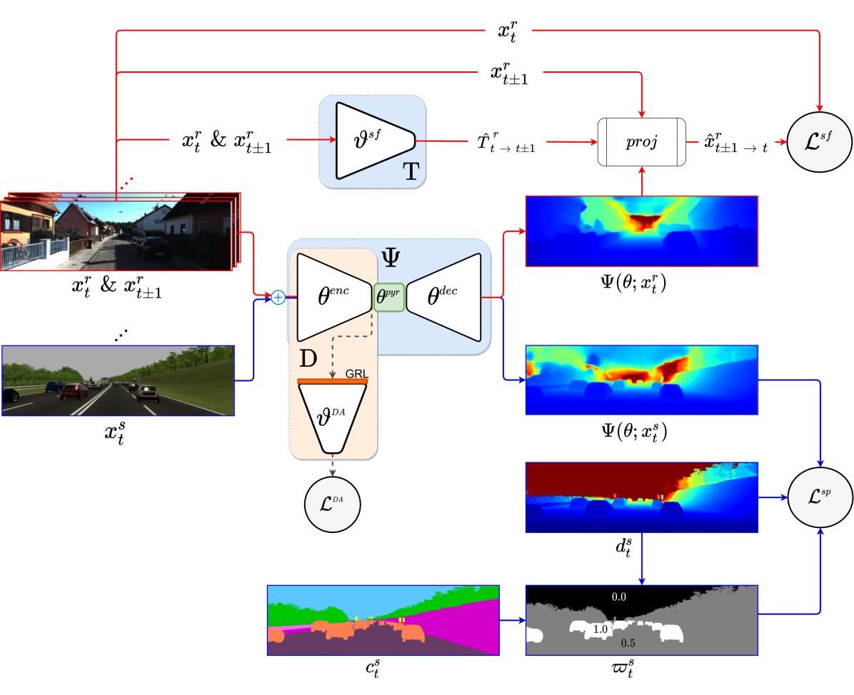
Figure 1: Training framework for MonoDEVSNet, i.e., ${\Psi(\theta;x)}$. We show the involved images, GT, weights, and losses. Red and blue lines are paths of real and virtual-world data, respectively. The discontinuous line is a common path.

III-B MonoDEVSNet architecture: ${\Psi(\theta;x)}$

MonoDEVSNet, i.e., our ${\Psi(\theta;x)}$, is composed of three main blocks: a encoding block of weights $\theta^{\mbox{{\scriptsize enc}}}$, a multi-scale pyramidal block, $\theta^{\mbox{{\scriptsize pyr}}}$, and a decoding block inspired in [23], $\theta^{\mbox{{\scriptsize dec}}}$. Therefore, the total set of weights is $\theta=\{\theta^{\mbox{{\scriptsize enc}}},\theta^{\mbox{{\scriptsize pyr}}},\theta^{\mbox{{\scriptsize dec}}}\}$. Here, $\theta^{\mbox{{\scriptsize enc}}}$ acts as a backbone of features. Moreover, since we aim at evaluating several encoders, the role of the multi-scale pyramid block is to adapt the bottleneck of the chosen encoder to the decoder. At testing time ${\Psi(\theta;x)}$ will process any real-world image $x$ acquired on-board the ego-vehicle, while at training time either $x\in X^{r}$ or $x\in X^{s}$.

III-C Problem formulation

Training ${\Psi(\theta;x)}$ consists in finding the optimum weight values, $\theta^{*}$, by solving the problem:

$${\theta^{*}=\min_{\theta}\mathcal{L}(\theta;X^{r},{X^{s}.Y^{s}})}\enspace,$$

where $\mathcal{L}$ is a loss function, and ${X^{s}.Y^{s}}$ indicates the use of the virtual-world frames with their GT. As we are going to detail, $\mathcal{L}$ relies on three different losses, namely, $\mathcal{L}^{\mbox{{\scriptsize sf}}},\mathcal{L}^{\mbox{{\scriptsize sp}}}$ and $\mathcal{L}^{\mbox{{\tiny DA}}}$. The loss $\mathcal{L}^{\mbox{{\scriptsize sf}}}$ focuses on training $\theta$ based on SfM self-supervision, thus, only relying on real-world data sequences. The SfM self-supervision is achieved with the support of a camera pose estimation task performed by a CNN, $\mathrm{T}$, of weights $\vartheta^{\mbox{{\scriptsize sf}}}$. Thus, we have ${\mathcal{L}^{\mbox{{\scriptsize sf}}}(\theta,\vartheta^{\mbox{{\scriptsize sf}}};{X^{r}})}$. The loss $\mathcal{L}^{\mbox{{\scriptsize sp}}}$ focuses on training $\theta$ with virtual-world supervision, in particular, using depth and semantic GT from virtual-world sequences. Therefore, we have ${\mathcal{L}^{\mbox{{\scriptsize sp}}}(\theta;{X^{s}.Y^{s}})}$. Finally, $\mathcal{L}^{\mbox{{\tiny DA}}}$ focuses on creating domain-invariant features $\theta^{\mbox{{\scriptsize enc}}}$ as part of $\theta$. In particular, we rely on a binary real/virtual domain-classifier CNN, $\mathrm{D}$, of weights $\{\theta^{\mbox{{\scriptsize enc}}},\vartheta^{\mbox{{\tiny DA}}}\}$. Thus, we have ${\mathcal{L}^{\mbox{{\tiny DA}}}(\theta^{\mbox{{\scriptsize enc}}},\vartheta^{\mbox{{\tiny DA}}};X^{r},X^{s})}$.

III-D SfM Self-supervised loss: ${\mathcal{L}^{\mbox{{\scriptsize sf}}}(\theta,\vartheta^{\mbox{{\scriptsize sf}}};{X^{r}})}$

Since we focus on improving MDE by the additional use of virtual-world data, for the SfM self-supervision we leverage from the state-of-the-art proposal in [23], which we briefly summarize here for the sake of completeness as:

$${\mathcal{L}^{\mbox{{\scriptsize sf}}}(\theta,\vartheta^{\mbox{{\scriptsize sf}}};X^{r})}=\sum_{t=2}^{N^{r}-1}P^{r}_{t}(\theta,\vartheta^{\mbox{{\scriptsize sf}}})+\lambda S^{r}_{t}(\theta)\enspace.$$ (1)

As introduced in [17], the term $\lambda S^{r}_{t}(\theta)$ is a constant weighted loss to force local smoothness on ${\Psi(\theta;x^{r}_{t})}$, taking into account the edges of $x^{r}_{t}$. The term $P^{r}_{t}(\theta,\vartheta^{\mbox{{\scriptsize sf}}})$ is the actual SfM-inspired loss. It involves the joint training of the depth estimation weights, $\theta$, and the relative camera pose estimation weights, $\vartheta^{\mbox{{\scriptsize sf}}}$. Figure 1 illustrates the CNN, $\mathrm{T}$, associated to these weights, which takes as input two consecutive frames, e.g., $(x^{r}_{t},x^{r}_{t+1})$, and outputs the pose transform (rotation and translation), ${\hat{T}}^{r}_{t\rightarrow t+1}=\mathrm{T}(\vartheta^{\mbox{{\scriptsize sf}}};x^{r}_{t},x^{r}_{t+1})$, between them. Then, as can be seen in Fig. 1, a projection module takes ${\hat{T}}^{r}_{t\rightarrow t+1},x^{r}_{t+1},$ and the depth estimation ${\Psi(\theta;x^{r}_{t})}$, to generate the synthesized frame $\hat{x}^{r}_{t+1\rightarrow t}(\theta,\vartheta^{\mbox{{\scriptsize sf}}})$ which, ideally, should match $x^{r}_{t}$. In fact, both frames adjacent to $x^{r}_{t}$ are considered for robustness. Thus, the SfM-inspired component of $\mathcal{L}^{\mbox{{\scriptsize sf}}}$ is defined as:

$$P^{r}_{t}(\theta,\vartheta^{\mbox{{\scriptsize sf}}})=\overline{cpe}(x^{r}_{t},\hat{x}^{r}_{t\pm 1\rightarrow t}(\theta,\vartheta^{\mbox{{\scriptsize sf}}}),x^{r}_{t\pm 1})\enspace,$$

where $cpe()$ is a pixelwise conditioned photo-metric error and $\overline{cpe}()$ its average over the pixels. Obtaining $cpe()$ starts by computing two pixelwise photo-metric error measurements, $pe(x^{r}_{t-1},x^{r}_{t},x^{r}_{t+1})$ and $pe(\hat{x}^{r}_{t-1\rightarrow t}(\theta,\vartheta^{\mbox{{\scriptsize sf}}}),x^{r}_{t},\hat{x}^{r}_{t+1\rightarrow t}(\theta,\vartheta^{\mbox{{\scriptsize sf}}}))$, where $pe(x^{r}_{-1},x^{r}_{0},x^{r}_{+1})=\min(pe(x^{r}_{0},x^{r}_{-1}),pe(x^{r}_{0},x^{r}_{+1}))$, and $pe(x^{r}_{A},x^{r}_{B})$ is the pixelwise photo-metric error between $x^{r}_{A}$ and $x^{r}_{B}$ defined in [17], i.e., based on local structural similarity (SSIM) and pixelwise photo-metric absolute differences between $x^{r}_{A}$ and $x^{r}_{B}$. Thus, $\min()$ applies pixelwise. Then, a pixelwise binary auto-mask [23] is computed as:

$$\varpi^{r}_{t}(x^{r}_{t},\hat{x}^{r}_{t\pm 1\rightarrow t}(\theta,\vartheta^{\mbox{{\scriptsize sf}}}),x^{r}_{t\pm 1})=$$

$$\big{[}pe(\hat{x}^{r}_{t-1\rightarrow t}(\theta,\vartheta^{\mbox{{\scriptsize sf}}}),x^{r}_{t},\hat{x}^{r}_{t+1\rightarrow t}(\theta,\vartheta^{\mbox{{\scriptsize sf}}}))<pe(x^{r}_{t-1},x^{r}_{t},x^{r}_{t+1})\big{]}_{\mbox{{\scriptsize I}}},$$

where $[\,\,]_{\mbox{{\scriptsize I}}}$ denotes the Iverson bracket applied pixelwise. Finally, $cpe()$ is computed as:

$$cpe(x^{r}_{t},\hat{x}^{r}_{t\pm 1\rightarrow t}(\theta,\vartheta^{\mbox{{\scriptsize sf}}}),x^{r}_{t\pm 1})=$$

$$\varpi^{r}_{t}(x^{r}_{t},\hat{x}^{r}_{t\pm 1\rightarrow t}(\theta,\vartheta^{\mbox{{\scriptsize sf}}}),x^{r}_{t\pm 1})\odot$$

$$pe(\hat{x}^{r}_{t-1\rightarrow t}(\theta,\vartheta^{\mbox{{\scriptsize sf}}}),x^{r}_{t},\hat{x}^{r}_{t+1\rightarrow t}(\theta,\vartheta^{\mbox{{\scriptsize sf}}}))\enspace,$$

where $\odot$ stands for pixelwise multiplication. The auto-mask $\varpi^{r}_{t}()$ conditions which pixels of $pe()$ are considered during the gradient computation of $\mathcal{L}^{\mbox{{\scriptsize sf}}}$. As explained in [23], the aim of $\varpi^{r}_{t}()$ is to remove, during training, the influence of pixels which remain the same between adjacent frames because they are assumed to often indicate SfM violations such as a static camera, objects moving as the camera, or low texture regions. The support of $\vartheta^{\mbox{{\scriptsize sf}}}$ is not needed at testing time.

III-E Supervised loss: ${\mathcal{L}^{\mbox{{\scriptsize sp}}}(\theta;{X^{s}.Y^{s}})}$

In this case, since we address an estimation problem and we have accurate GT, we base $\mathcal{L}^{\mbox{{\scriptsize sp}}}$ on the L1 metric. On the other hand, MDE is specially interesting to determine how far is the ego-vehicle from vehicles, pedestrians, etc. Accordingly, since $Y^{s}$ includes semantic class GT, we use it to increase the relevance of accurately estimating the depth for such major traffic protagonists. Moreover, since virtual-world depth maps are based on the Z-buffer involved on image rendering, the range of depth values available as GT tend to be over-optimistic even for active sensors such as LiDAR. For instance, there can be depth values larger than $300~{}m$ in the Z-buffer. Since we do not aim at estimating depth beyond a reasonable threshold (in $m$), $d^{\mbox{{\scriptsize max}}}$, to compute $\mathcal{L}^{\mbox{{\scriptsize sp}}}$ we will also discard pixels $p$ with $d^{s}_{t}(p)\geq d^{\mbox{{\scriptsize max}}}$. For each $x^{s}_{t}$, both the semantic class relevance and the out-of-range depth values, can be codified as real-valued weights running on $[0,1]$ and arranged on a mask, $\varpi^{s}_{t}$. Thus, $\varpi^{s}_{t}$ depends on $d^{s}_{t},d^{\mbox{{\scriptsize max}}},$ and $c^{s}_{t}$. However, contrarily to $\varpi^{r}_{t}()$, we can compute $\varpi^{s}_{t}$ offline, i.e., before starting the training process. Taking all these details into account, we define our supervised loss as:

$${\mathcal{L}^{\mbox{{\scriptsize sp}}}(\theta;{X^{s}.Y^{s}})}=\sum_{t=1}^{N^{s}}\|{\varpi^{s}_{t}\odot({\Psi(\theta;x^{s}_{t})}-d^{s}_{t})}\|_{1}\enspace.$$ (2)

III-F Domain adaptation loss: ${\mathcal{L}^{\mbox{{\tiny DA}}}(\theta^{\mbox{{\scriptsize enc}}},\vartheta^{\mbox{{\tiny DA}}};X^{r},X^{s})}$

As can be seen in Fig. 1, we aim at learning depth features, $\theta^{\mbox{{\scriptsize enc}}}$, so that it cannot be distinguished whether they were generated from a real-world input frame (target domain) or a virtual-world one (source domain); in other words, learning a domain invariant $\theta^{\mbox{{\scriptsize enc}}}$. Taking into account that we do not have accurate depth GT in the target domain, while we do have it for the source domain, we need to apply an unsupervised DA technique to train $\theta^{\mbox{{\scriptsize enc}}}$. In addition, as part of $\theta$, the training of $\theta^{\mbox{{\scriptsize enc}}}$ must result on an accurate ${\Psi(\theta;x)}$. Achieving this accuracy and domain invariance are adversarial goals. Accordingly, we propose to use the Gradient-Reversal-Layer (GRL) idea introduced in [43], which, up to the best of our knowledge, has not been applied before for DA in the context of MDE. In this approach, the domain invariance of $\theta^{\mbox{{\scriptsize enc}}}$ is measured by a binary target/source domain-classifier CNN, $\mathrm{D}$, of weights $\{\theta^{\mbox{{\scriptsize enc}}},\vartheta^{\mbox{{\tiny DA}}}\}$. In [43], a logistic loss is proposed to train the domain classifier. In our case, this is set as:

$${\mathcal{L}^{\mbox{{\tiny DA}}}(\theta^{\mbox{{\scriptsize enc}}},\vartheta^{\mbox{{\tiny DA}}};X^{r},X^{s})}=$$ (3)

$$\sum_{t=1}^{N^{r}}\log(\mathrm{D}(\theta^{\mbox{{\scriptsize enc}}},\vartheta^{\mbox{{\tiny DA}}};x^{r}_{t}))+\sum_{t=1}^{N^{s}}\log(1-\mathrm{D}(\theta^{\mbox{{\scriptsize enc}}},\vartheta^{\mbox{{\tiny DA}}};x^{s}_{t}))\enspace,$$

where we assume that $\mathrm{D}(\theta^{\mbox{{\scriptsize enc}}},\vartheta^{\mbox{{\tiny DA}}};x)$ outputs 1 if $x\in X^{r}$ and 0 if $x\in X^{s}$. The GRL has no parameters and connects $\theta^{\mbox{{\scriptsize enc}}}$ with $\vartheta^{\mbox{{\tiny DA}}}$ (see Fig. 1). Its behavior is exactly as explained in [43]. This means that during forward passes of training, it acts as an identity function, while, during back-propagation, it reverses the gradient vector passing through it. Both the GRL and $\vartheta^{\mbox{{\tiny DA}}}$ are required at training time, but not at testing time.

III-G Overall training procedure

Algorithm 1 summarizes the steps to compute the needed gradient vectors for mini-batch optimization. In particular, we need the gradients related to MonoDEVSNet weights, $\theta=\{\theta^{\mbox{{\scriptsize enc}}},\theta^{\mbox{{\scriptsize pyr}}},\theta^{\mbox{{\scriptsize dec}}}\}$, and the weights of the auxiliary tasks, i.e., $\vartheta^{\mbox{{\scriptsize sf}}}$ for SfM self-supervision, and $\vartheta^{\mbox{{\tiny DA}}}$ for DA. Regarding gradient computation, we do not need to distinguish $\theta^{\mbox{{\scriptsize pyr}}}$ from $\theta^{\mbox{{\scriptsize dec}}}$, so we define $\theta^{\mbox{{\scriptsize pyde}}}=\{\theta^{\mbox{{\scriptsize pyr}}},\theta^{\mbox{{\scriptsize dec}}}\}$. In Alg. 1, we introduce an equalizing factor between supervised and self-supervised losses, $\omega^{\mbox{{\scriptsize sf}}}\in\mathbb{R}$, which aims at avoiding one loss dominating over the other. A priori, we could set a constant factor. However, in practice, we have found that having an adaptive value is more useful. Therefore, inspired by the GradNorm idea [58], we use the ratio between the supervised and self-supervised losses. Algorithm 1 also introduces the scaling factor $\omega^{\mbox{{\tiny DA}}}\in\mathbb{R}$ which, following [43], controls the trade-off between optimizing $\theta^{\mbox{{\scriptsize enc}}}$ to obtain an accurate ${\Psi(\theta;x)}$ model versus being domain invariant. Finally, ${\mathcal{L}^{\mbox{{\tiny DA}}}(\theta^{\mbox{{\scriptsize enc}}},\vartheta^{\mbox{{\tiny DA}}};\emptyset,X^{s}_{B})}$ and ${\mathcal{L}^{\mbox{{\tiny DA}}}(\theta^{\mbox{{\scriptsize enc}}},\vartheta^{\mbox{{\tiny DA}}};X^{r}_{B},\emptyset)}$ indicate whether this loss must be computed only using virtual- or real-world data, respectively.

Algorithm 1 Computing the gradients ${\Delta_{\theta^{\mbox{{\scriptsize enc}}}}}$, ${\Delta_{\theta^{\mbox{{\scriptsize pyde}}}}}$, ${\Delta_{\vartheta^{\mbox{{\scriptsize sf}}}}}$, ${\Delta_{\vartheta^{\mbox{{\tiny DA}}}}}$ for a mini-batch $X^{r}_{B}\subset X^{r},X^{s}_{B}.Y^{s}_{B}\subset X^{s}.Y^{s}$. ${\nabla_{\xi_{i}}}F(\xi_{1},\xi_{2})$ refers to back-propagation on $F(\xi_{1},\xi_{2})$ with respect to weights $\xi_{i}\subset\xi_{1}\cup\xi_{2}$. $\emptyset$ is the empty set.

Forward Passes with $\{X^{s}_{B},Y^{s}_{B}\}$

$$\ell^{\mbox{{\scriptsize sp}}}(\theta)\leftarrow {\mathcal{L}^{\mbox{{\scriptsize sp}}}(\theta;{X^{s}_{B}.Y^{s}_{B}})}$$

$$\ell^{\mbox{{\tiny DA}},s}(\theta^{\mbox{{\scriptsize enc}}},\vartheta^{\mbox{{\tiny DA}}})\leftarrow \omega^{\mbox{{\tiny DA}}}{\mathcal{L}^{\mbox{{\tiny DA}}}(\theta^{\mbox{{\scriptsize enc}}},\vartheta^{\mbox{{\tiny DA}}};\emptyset,X^{s}_{B})}$$

Back-propagation for Supervision & DA

$${\Delta^{s}_{\theta^{\mbox{{\scriptsize pyde}}}}}\leftarrow {\nabla_{\theta^{\mbox{{\scriptsize pyde}}}}}\ell^{\mbox{{\scriptsize sp}}}(\theta)$$

$${\Delta^{s}_{\theta^{\mbox{{\scriptsize enc}}}}}\leftarrow {\nabla_{\theta^{\mbox{{\scriptsize enc}}}}}(\ell^{\mbox{{\scriptsize sp}}}(\theta)-\ell^{\mbox{{\tiny DA}},s}(\theta^{\mbox{{\scriptsize enc}}},\vartheta^{\mbox{{\tiny DA}}}))$$

$${\Delta^{s}_{\vartheta^{\mbox{{\tiny DA}}}}}\leftarrow {\nabla_{\vartheta^{\mbox{{\tiny DA}}}}}\ell^{\mbox{{\tiny DA}},s}(\theta^{\mbox{{\scriptsize enc}}},\vartheta^{\mbox{{\tiny DA}}})$$

Forward Passes with $X^{r}_{B}$

$$\ell^{\mbox{{\scriptsize sf}}}(\theta,\vartheta^{\mbox{{\scriptsize sf}}})\leftarrow {\mathcal{L}^{\mbox{{\scriptsize sf}}}(\theta,\vartheta^{\mbox{{\scriptsize sf}}};X^{r}_{B})}$$

$$\ell^{\mbox{{\tiny DA}},r}(\theta^{\mbox{{\scriptsize enc}}},\vartheta^{\mbox{{\tiny DA}}})\leftarrow \omega^{\mbox{{\tiny DA}}}{\mathcal{L}^{\mbox{{\tiny DA}}}(\theta^{\mbox{{\scriptsize enc}}},\vartheta^{\mbox{{\tiny DA}}};X^{r}_{B},\emptyset)}$$

Back-propagation for Self-supervision & DA

$${\Delta^{r}_{\theta^{\mbox{{\scriptsize pyde}}}}}\leftarrow {\nabla_{\theta^{\mbox{{\scriptsize pyde}}}}}\ell^{\mbox{{\scriptsize sf}}}(\theta,\vartheta^{\mbox{{\scriptsize sf}}})$$

$${\Delta^{r}_{\theta^{\mbox{{\scriptsize enc}}}}}\leftarrow {\nabla_{\theta^{\mbox{{\scriptsize enc}}}}}(\ell^{\mbox{{\scriptsize sf}}}(\theta,\vartheta^{\mbox{{\scriptsize sf}}})-\ell^{\mbox{{\tiny DA}},r}(\theta^{\mbox{{\scriptsize enc}}},\vartheta^{\mbox{{\tiny DA}}}))$$

$${\Delta^{r}_{\vartheta^{\mbox{{\tiny DA}}}}}\leftarrow {\nabla_{\vartheta^{\mbox{{\tiny DA}}}}}\ell^{\mbox{{\tiny DA}},r}(\theta^{\mbox{{\scriptsize enc}}},\vartheta^{\mbox{{\tiny DA}}})$$

Setting the final gradient vectors

$${\Delta_{\vartheta^{\mbox{{\scriptsize sf}}}}}\leftarrow {\nabla_{\vartheta^{\mbox{{\scriptsize sf}}}}}\ell^{\mbox{{\scriptsize sf}}}(\theta,\vartheta^{\mbox{{\scriptsize sf}}})$$

$${\Delta_{\vartheta^{\mbox{{\tiny DA}}}}}\leftarrow {\Delta^{s}_{\vartheta^{\mbox{{\tiny DA}}}}}+{\Delta^{r}_{\vartheta^{\mbox{{\tiny DA}}}}}$$

$$\omega^{\mbox{{\scriptsize sf}}}\leftarrow \ell^{\mbox{{\scriptsize sp}}}(\theta)/\ell^{\mbox{{\scriptsize sf}}}(\theta,\vartheta^{\mbox{{\scriptsize sf}}})$$

$${\Delta_{\theta^{\mbox{{\scriptsize pyde}}}}}\leftarrow {\Delta^{s}_{\theta^{\mbox{{\scriptsize pyde}}}}}+\omega^{\mbox{{\scriptsize sf}}}{\Delta^{r}_{\theta^{\mbox{{\scriptsize pyde}}}}}$$

$${\Delta_{\theta^{\mbox{{\scriptsize enc}}}}}\leftarrow {\Delta^{s}_{\theta^{\mbox{{\scriptsize enc}}}}}+\omega^{\mbox{{\scriptsize sf}}}{\Delta^{r}_{\theta^{\mbox{{\scriptsize enc}}}}}$$

III-H Absolute depth computation

The virtual-world supervised data trains ${\Psi(\theta;x)}$ on absolute depth values, while the real-world SfM self-supervised data trains ${\Psi(\theta;x)}$ on relative depth values. Thanks to the unsupervised DA, the depth features $\theta^{\mbox{{\scriptsize enc}}}$ are trained to be domain invariant. However, according to our experiments, this is not sufficient for ${\Psi(\theta;x)}$ producing accurate absolute depth values at testing time. Fortunately, thanks to the use of virtual-world data, we can still compute a global scaling factor, $\psi\in\mathbb{R}$, so that $\psi{\Psi(\theta;x)}$ is accurate in absolute depth terms. For that, we assume that the sequences in $X^{s}$ are acquired with a camera analogous to the one used to acquire the sequences in $X^{r}$. Here analogous refers to using the same number of pixels, field of view, frame rate, and mounted on-board in similar heading directions. Note that simulators are flexible enough for setting these camera parameters as needed. Accordingly, we train a ${\Psi(\theta;x)}$ model using only data from $X^{s}$ and SfM self-supervision, i.e. as if we would not have supervision for $X^{s}$. Then, we find the median depth value produced by this model on the virtual-world data, $\hat{d}^{s,\mbox{{\scriptsize m}}}\in\mathbb{R}$. Finally, we set $\psi=d^{s,\mbox{{\scriptsize m}}}/\hat{d}^{s,\mbox{{\scriptsize m}}}$, where $d^{s,\mbox{{\scriptsize m}}}\in\mathbb{R}$ is the median depth value of the GT. This pre-processing step is performed once and the model discarded afterwards. Other works apply a similar approach [19, 23, 39, 51, 21] but relying on LiDAR data as GT reference, while we only rely on virtual-world data.

IV Experimental Results

We start by defining the datasets and evaluation metrics used in our experiments. After, we provide relevant implementation and training details of MonoDEVSNet. Finally, we present and discuss our quantitative and qualitative results, comparing them with those from previous literature as well as performing an ablative analysis over MonoDEVSNet components.

IV-A Datasets and evaluation metrics

We use publicly available datasets and metrics which are de facto standards in MDE research. In particular, we use KITTI Raw (KR) [59] and Virtual KITTI (VK) [29] as real- and virtual-world sequences, respectively. We follow Zhou et al. [19] training-testing split. From the training split we select 12K monocular triplets, i.e., samples of the form $\{x^{r}_{t-1},x^{r}_{t},x^{r}_{t+1}\}$. The testing split consists of 697 isolated images with LiDAR-based GT, actually introduced by Eigen et al. [5]. In addition, for considering the semantic content of the images in the analysis of results, we also use KITTI Stereo 2015 (KS) [60] for testing. This dataset consists of 200 isolated images with enhanced depth maps and semantic labels. VK is used only for training, we also use 12K monocular triplets (non-rotated camera subset) with associated depth GT. In this case, the triplets are used to calibrate the global scaling factor $\psi$ (see Sect. III-H), while for actual training supervision only 12K isolated frames are used. As the depth GT of VK ranges up to $\sim 655$m, to match the range of KR’s LiDAR-based GT, we clip it to $80$m ($d^{\mbox{{\scriptsize max}}}$). VK includes similar weather conditions as KR/KS, and adds situations with fog, overcast, and rain, as well as sunrise and sunset illumination.

As is common practice since [17], we use Make3D dataset [61] for assessing generalization. It contains photographs of urban and natural areas. Thus, Make3D shows views and content pretty much different from those on-board a vehicle as KR, KS, and VK. The images come with depth GT acquired by a 3D scanner. There are 534 images with depth GT, organized in a standard split of 400 for training and 134 for testing. We use the latter, since we rely on Make3D only for testing.

In order to assess quantitative MDE results, we use the standard metrics introduced by Eigen et al. [5], i.e., the average absolute relative error (abs-rel), the average squared relative error (sq-rel), the root mean square error (rms), and the rms log error (rms-log). For these metrics, the lower the better. In addition, the accuracy (termed as $\delta$) under a threshold $\tau\in\{1.25,1.25^{2},1.25^{3}\}$ is also used as metric. In this case, the higher the better. The abs-rel error and the ${\delta<\tau}$ are percentage measurements, sq-rel and rms are reported in meters, and rms-log is similar (reported in meters) to rms but applied to logarithm depth values.

These metrics are applied to absolute depth values for MDE models trained with depth supervision coming from either LiDAR [5, 6, 7, 8, 9, 10, 11, 12, 13, 14, 26], stereo [15, 16, 17, 23, 18], real-world stereo and virtual-world depth [37, 38], or stereo and LiDAR [24, 25]. However, MDE models trained on pure SfM self-supervision can only estimate depth in relative terms, i.e., up to scale. Moreover, the scale factor varies from image to image, a problem known as scale inconsistency. In this case, before computing the above metrics, it is applied a per-image correction factor computed at testing time [19, 20, 21, 23, 51, 39]. In particular, given a test image $x$ with GT and estimated depth $d(x)$ and $\hat{d}(x)$, respectively, the common practice consists of computing a scale $\psi(x)\in\mathbb{R}$ as the ratio $\mbox{median}(d(x))/\mbox{median}(\hat{d}(x))$, and then compare $\psi(x)\hat{d}(x)$ with $d(x)$. On the other hand, SfM self-supervision with the help of additional information can train models able to produce absolute scale in testing time. For instance, [22] uses the ego-vehicle speed and, in fact, virtual-world supervision can help too [35, 36]. The latter approach is the one followed in this paper, especially thanks to the procedure presented in Sect. III-H. Therefore, ${\Psi(\theta;x)}$ will be evaluated in relative scale terms, and $\psi{\Psi(\theta;x)}$ in absolute terms. Please, note that our $\psi\in\mathbb{R}$ scaling factor is constant for all the evaluated images and computed at training time. In the following, when presenting quantitative results, we will make clear if they are in relative or absolute terms.

IV-B Implementation details

We start by selecting the actual CNN layers to implement ${\Psi(\theta;x)}$. Since we leverage the SfM self-supervision idea from [23], a straightforward implementation would be to use its ResNet-based architecture as it is. However, the High-Resolution Network (HRNet) architecture [62], exhibits better accuracy in visual tasks such as semantic segmentation and object detection, suggesting that it can be a better backbone than ResNet. Thus, we decided to start our experiments by comparing ResNet and HRNet backbones using the SfM self-supervision framework provided in [23]. In particular, we assess different ResNet/HRNet architectures for $\theta^{\mbox{{\scriptsize enc}}}$, while using the proposal in [23] for $\theta^{\mbox{{\scriptsize dec}}}$. Then, when using ResNet we have $\theta^{\mbox{{\scriptsize pyr}}}=\emptyset$, while for HRNet $\theta^{\mbox{{\scriptsize pyr}}}$ consists of pyramidal layers adapting the $\theta^{\mbox{{\scriptsize enc}}}$ and $\theta^{\mbox{{\scriptsize dec}}}$ CNN architectures under test. For these experiments, we rely on KR. Table I shows the accuracy (in relative scale terms) of the tested variants and their number of weights. We see how HRNet outperforms ResNet, being HRNet-W48 the best. Indeed, HRNet is slower than ResNet, and HRNet-W48 is the one requiring more GFLOPS by far. However, at this stage of our research we target the architecture which potentially can provide higher depth estimation accuracy. Thus, for our following experiments, we will rely on HRNet-W48 although being the heaviest. We show the corresponding pyramidal architecture of $\theta^{\mbox{{\scriptsize pyr}}}$ in Fig. 2. It is composed of five blocks ($\mathcal{P}_{i}$), where each block is a pipeline of three consecutive layers consisting of convolution, batch normalization, and ReLU. As a deep learning framework, we use PyTorch 1.5v [63].

TABLE I: Comparing ResNet and HRNet as backbone for ${\Psi(\theta;x)}$, training only on SfM self-supervision (relative scale) using the framework in [23]. MW column stands for millions of $\theta^{\mbox{{\scriptsize enc}}}$ weights to be learnt. FPS stands for frames per second as required by ${\Psi(\theta;x)}$ to process $x$, while GFLOPS refers to the giga floating-point operations per second required by $\theta^{\mbox{{\scriptsize enc}}}$; in both cases using an NVIDIA RTX 2080Ti GPU. The $1.25^{n}$ columns, $n\in\{1,2\}$, refer to the $\tau$ in the usual $\delta<\tau$ accuracy metrics. In all the tables of Sect. IV, bold stands for best and underline for second-best. $(^{*})$ Currently, HRNet branches do not run in parallel in PyTorch, thus, compromising speed.

$\theta^{\mbox{{\scriptsize enc}}}$ Backb.	MW	GFLOPS	FPS	abs-rel	sq-rel	rms	$1.25$	$1.25^{2}$
ResNet-18	11.6	4.47	141.2	0.115	0.882	4.701	0.879	0.961
ResNet-50	25.5	10.14	77.06	0.110	0.831	4.642	0.883	0.962
ResNet-101	44.5	19.29	43.26	0.110	0.809	4.712	0.878	0.960
ResNet-152	60.2	28.47	30.71	0.107	0.800	4.629	0.885	0.962
HRNet-W18	9.5	8.29	$15.79^{*}$	0.107	0.846	4.671	0.887	0.962
HRNet-W32	29.3	19.50	$15.53^{*}$	0.107	0.881	4.794	0.886	0.961
HRNet-W48	65.3	40.04	$15.48^{*}$	0.105	0.791	4.590	0.888	0.963

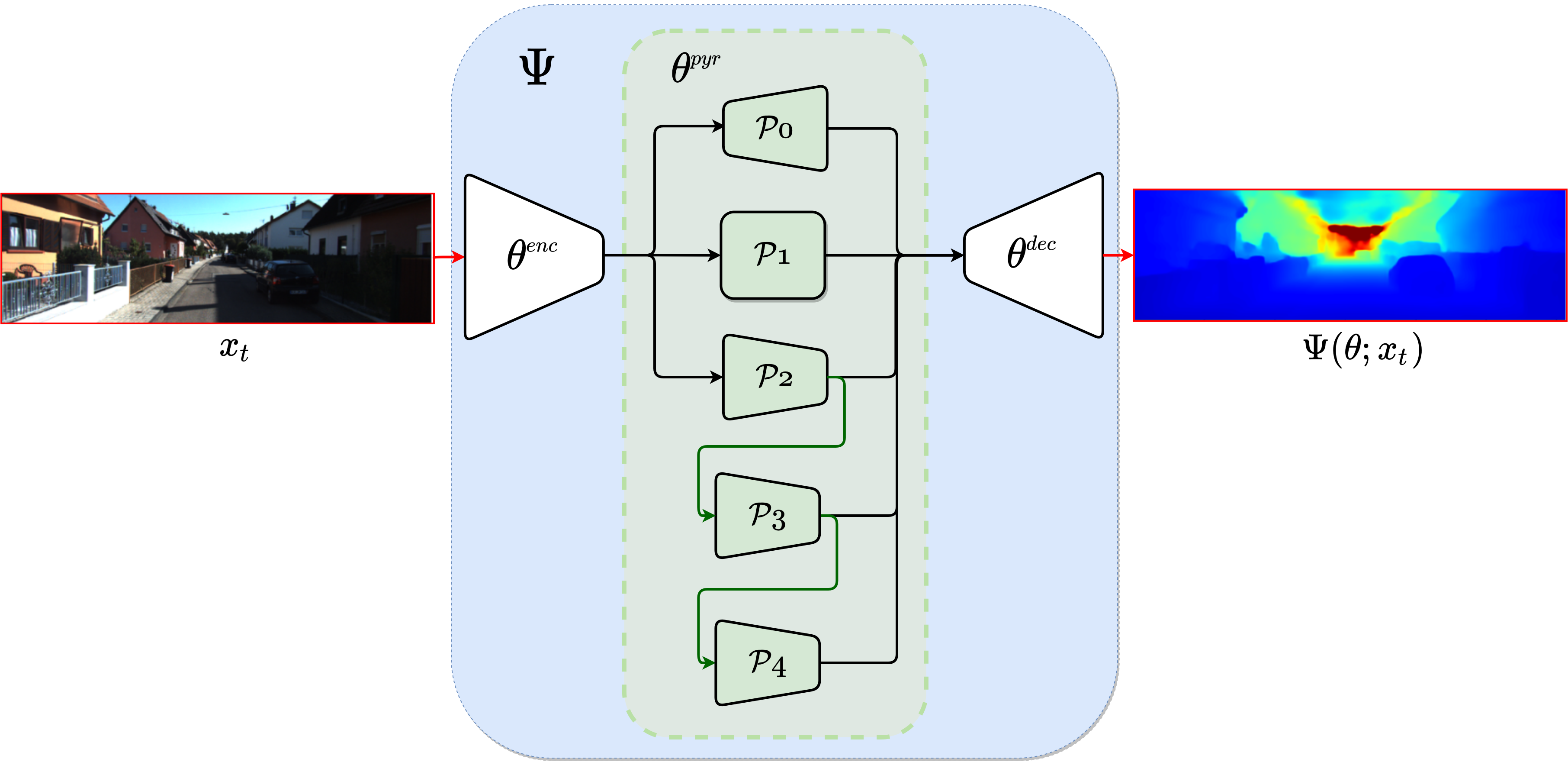
Figure 2: Pyramidal architecture of $\theta^{\mbox{{\scriptsize pyr}}}$.

In order to train the camera pose estimation network, $\mathrm{T}(\vartheta^{\mbox{{\scriptsize sf}}};x^{r}_{t},x^{r}_{t\pm 1})$, we follow [23] but using ResNet-50 instead of ResNet-18 since the former is more accurate. Four convolutional layers are used to convert the ResNet-50 bottleneck features to the 6-DoF relative pose vector (3D translation and rotation). For training the classification block of $\mathrm{D}(\theta^{\mbox{{\scriptsize enc}}},\vartheta^{\mbox{{\tiny DA}}};x)$, i.e., $\vartheta^{\mbox{{\tiny DA}}}$, we use a standard classification pipeline based on convolutions, ReLU and fully connected layers. Finally, we remark that these networks are not required at testing time.

IV-C Training details

The input images are processed (at training and testing time) at a resolution of ${640\times 192}$ ($W\times H$), where LANCZOS interpolation is performed from the ${\sim 1242\times 375}$ original resolution. As optimizer, we use Adam [64] with learning rate ${lr=10^{-4}}$, and the rest of its hyper-parameters set to default values. The weights $\theta^{\mbox{{\scriptsize enc}}}$ are initialized from available ImageNet [65] pre-training, $\theta^{\mbox{{\scriptsize pyr}}},\theta^{\mbox{{\scriptsize dec}}}$, and $\vartheta^{\mbox{{\tiny DA}}}$ are randomly initialized with Kaiming weights, while the ResNet-50 part of $\vartheta^{\mbox{{\scriptsize sf}}}$ is also initialized with ImageNet and the rest (convolutional layers to output the pose vector) following Kaiming. The mini-batch size is of 16 images, 50%/50% from real/virtual domains. To minimize over-fitting, we apply standard data augmentation such as horizontal flip, a 50% chance of random brightness, contrast, saturation, and hue jitter with ranges of $\pm 0.2$, $\pm 0.2$, $\pm 0.2$, and $\pm 0.1$, respectively. Remaining hyper-parameters were set as $\lambda=0.001$ in Eq. (1), $\omega^{\mbox{{\tiny DA}}}=10$ in Alg. 1, and in Eq. (4) our mask $\varpi^{s}_{t}$ is set to have values of $1.0$ for traffic participants (vehicles, pedestrians, etc.), $0.5$ for static infrastructure (buildings, road, vegetation, etc.), and $0.0$ for the sky and pixels with depth over $d^{\mbox{{\scriptsize max}}}$ (here $80$m).

IV-D Results and discussion

IV-D1 Relative depth assessment

We start by assessing MDE in relative terms. Table II presents MonoDEVSNet results (Ours) and those from previous works based on SfM self-supervision. From this table we can draw several observations. Regarding DA, MonoDEVSNet (VK_v1) outperforms $S^{3}$Net (VK_v1) in all metrics. The new version of VK (VK_v2) allows us to obtain even better results. MonoDEVSNet with virtual-world supervision outperforms the version with only SfM self-supervision (best result in Table I) in all metrics, no matter the VK version we use. Overall, MonoDEVSNet outperforms most previous methods, being on pair with [51].

TABLE II: Relative depth results up to $80$m on the (KR) Eigen et al. [5] testing split. These methods rely on SfM self-supervision. In addition, methods in gray use DA supported by VK. ${(^{1})}$ MonoDepth2 is based only on SfM self-supervision.

Method	abs-rel	sq-rel	rms	rms-log	$1.25$	$1.25^{2}$	$1.25^{3}$
[19] (Zhou et al.)	0.183	1.595	6.709	0.270	0.734	0.902	0.959
[20] GeoNet	0.149	1.060	5.567	0.226	0.796	0.935	0.975
[23] MonoDepth21	0.115	0.903	4.863	0.193	0.877	0.959	0.981
[21] (Zhao et al.)	0.113	0.704	4.581	0.184	0.871	0.961	0.984
[51] (Guizilini et al.)	0.102	0.698	4.381	0.178	0.896	0.964	0.984
[39] $S^{3}$Net (VK_v1)	0.124	0.826	4.981	0.200	0.846	0.955	0.982
MonoDEVSNet / VK_v1	0.105	0.753	4.389	0.179	0.890	0.965	0.983
MonoDEVSNet / VK_v2	0.102	0.685	4.303	0.178	0.894	0.966	0.984

IV-D2 Absolute depth assessment

While assessing depth in relative terms is a reasonable option to compare methods purely based on SfM self-supervision, the most relevant evaluation is in terms of absolute depth. These are presented in Table III. The first (top) block of this table shows results based on depth supervision from LiDAR, thus, a priori they can be thought of as upper-bounds for methods based on self-supervision. The second block shows methods that only use virtual-world supervision. The third and fourth (bottom) blocks show results based on stereo and SfM self-supervision, respectively. Methods in gray use DA supported by VK. We can draw several observations from this table. MonoDEVSNet (Ours) is the best performing among those leveraging supervision from VK_v1 and, consistently with the results on relative depth, by using VK_v2 we improve MonoDEVSNet results. In fact, MonoDEVSNet based on VK_v2 outperforms all self-supervised methods, including those using stereo rigs instead of monocular systems. We are not yet able to reach the performance of the best methods supervised with LiDAR data. However, it is clear that our proposal is able to successfully combine real-world SfM self-supervision and virtual-world supervision. Thus, we think it is worth to keep this line of research until reaching the LiDAR-based upper-bounds.

TABLE III: Absolute depth results up to $80$m on the (KR) Eigen et al. [5] testing split. We divide the results into four blocks. From top to bottom, the blocks refer to: methods based on LiDAR supervision, only virtual-world supervision, stereo self-supervision, SfM self-supervision. In these blocks, we remark best and second-best results per block. Methods in gray use DA supported by VK. We remark some additional comments: ${(^{1})}$ in addition to LiDAR supervision, it also uses stereo self-supervision; ${(^{2})}$ it uses stereo and SfM self-supervision; ${(^{3})}$ in this case, the MDE network is pre-trained on Cityscapes dataset [66] and then fine-tuned on KITTI.

Method	abs-rel	sq-rel	rms	rms-log	$1.25$	$1.25^{2}$	$1.25^{3}$
[5] (Eigen et al.)	0.203	1.548	6.307	0.282	0.702	0.890	0.890
[6] (Liu et al.)	0.217	1.841	6.986	0.289	0.647	0.882	0.961
[9] (Cao et al.)	0.115	N/A	4.712	0.198	0.887	0.963	0.982
[24] (Kuzni. et al.)1	0.113	0.741	4.621	0.189	0.862	0.960	0.986
[13] (Xu et al.)	0.122	0.897	4.677	N/A	0.818	0.954	0.985
[11] (Gurram et al.)	0.100	0.601	4.298	0.174	0.874	0.966	0.989
[10] DORN	0.098	0.582	3.666	0.160	0.899	0.967	0.986
[14] VNL	0.072	N/A	3.258	0.117	0.938	0.990	0.998
[36] AdaDepth / VK_v1	0.167	1.257	5.578	0.237	0.771	0.922	0.971
[35] $T^{2}$Net / VK_v1	0.174	1.410	6.046	0.253	0.754	0.916	0.966
[16] (Garg et al.)	0.169	1.512	5.763	0.236	0.836	0.935	0.968
[18] SuperDepth	0.112	0.875	4.958	0.207	0.852	0.947	0.977
[23] MonoDepth2	0.109	0.873	4.960	0.209	0.864	0.948	0.975
[23] MonoDepth22	0.106	0.806	4.630	0.193	0.876	0.958	0.980
[37] GASDA / VK_v1	0.120	1.022	5.162	0.215	0.848	0.944	0.974
[38] SharinGAN / VK_v1	0.116	0.939	5.068	0.203	0.850	0.948	0.978
[22] PackNet-SfM	0.111	0.829	4.788	0.199	0.864	0.954	0.980
[22] PackNet-SfM3	0.108	0.803	4.642	0.195	0.875	0.958	0.980
MonoDEVSNet / VK_v1	0.108	0.775	4.464	0.188	0.875	0.961	0.982
MonoDEVSNet / VK_v2	0.104	0.721	4.396	0.185	0.880	0.962	0.983

TABLE IV: Absolute depth ablative results of MonoDEVSNet (VK_v2) up to $80$m on the (KR) Eigen testing split [5]. Rows 1-6 show the progressive use of the components of our proposal (each row adds a new component). ${50/50}$ refers to mini-batches of 50% real-world samples and 50% or virtual-world ones; not using ${50/50}$ (rows 1-2) means that we alternate mini-batches of pure real- or virtual-world samples. Row 7 corresponds to a simplification of the SfM self-supervised loss. ${\vartheta^{\mathcal{G}}}$ (rows 8-9) refers to a GAN-based DA approach. LB (lower bound, row 10) indicates the use of only virtual-world data. UB (upper bound, row 12) indicates the use of KITTI LiDAR-based supervision instead of virtual-world data. Rows 11 and 13 show the difference of our best model (All) with respect to LB and UB, respectively. ${\uparrow D}$ means that All is $D$ units better, while ${\downarrow D}$ means that it is $D$ units worse. All/W18 (row 14) and All/W32 (row 15) refer to using the All configuration by relying on HRNet-W18 and HRNet-W32, respectively.

Configuration	abs-rel	sq-rel	rms	rms-log	$1.25$	$1.25^{2}$	$1.25^{3}$
1. $\{X^{r},X^{s}.Y^{s}\}$	0.368	2.601	8.025	0.514	0.080	0.478	0.883
2. $+\psi$	0.140	0.876	4.915	0.217	0.828	0.950	0.980
3. $+{50/50}$	0.128	0.880	4.618	0.198	0.844	0.957	0.982
4. $+\vartheta^{\mbox{{\tiny DA}}}$	0.110	0.724	4.450	0.187	0.873	0.960	0.983
5. $+\omega^{\mbox{{\scriptsize sf}}}$	0.106	0.716	4.441	0.188	0.876	0.962	0.982
6. $+\varpi^{s}_{t}$ (All)	0.104	0.721	4.396	0.185	0.880	0.962	0.983
7. Simplified $\mathcal{L}^{\mbox{{\scriptsize sf}}}$	0.105	0.736	4.471	0.190	0.875	0.960	0.981
8. All$+{\vartheta^{\mathcal{G}}};-\vartheta^{\mbox{{\tiny DA}}}$	0.119	0.809	4.654	0.196	0.857	0.958	0.982
9. All$+{\vartheta^{\mathcal{G}}}$	0.106	0.748	4.503	0.191	0.873	0.959	0.981
10. LB	0.165	1.280	5.628	0.248	0.777	0.916	0.965
11. $\uparrow$All vs. $\downarrow$LB	$\uparrow$0.061	$\uparrow$0.559	$\uparrow$1.232	$\uparrow$0.063	$\uparrow$0.103	$\uparrow$0.046	$\uparrow$0.018
12. UB	0.088	0.583	3.978	0.164	0.906	0.970	0.986
13. $\uparrow$All vs. $\downarrow$UB	$\downarrow$0.016	$\downarrow$0.138	$\downarrow$0.418	$\downarrow$0.021	$\downarrow$0.026	$\downarrow$0.008	$\downarrow$0.003
14. All/W18	0.109	0.773	4.524	0.190	0.871	0.960	0.982
15. All/W32	0.107	0.754	4.510	0.188	0.875	0.960	0.982

IV-D3 Ablative analysis of MonoDEVSNet

It is also worth to analyze the contribution of the main components of our proposal. In rows 1-6 of Table IV, we add one component at a time showing performance for absolute depth. The 1st row corresponds to using the real-world data with SfM self-supervision and the virtual-world images with only depth supervision, i.e., without using neither semantic supervision ($\varpi^{s}_{t}$), nor gradient equalization ($\omega^{\mbox{{\scriptsize sf}}}$), nor domain adaptation ($\vartheta^{\mbox{{\tiny DA}}}$), nor mixed mini-batches (${50/50}$), nor the global scaling factor ($\psi$). By comparing 1st and 2nd rows (i.e., w/o $\psi$ and w/ $\psi$, resp.), we can see how relevant is obtaining a good global scaling factor to output absolute depth. In fact, adding $\psi$ to the virtual-world depth supervision shows the higher improvement among all the components of our proposal. Then, using mixed mini-batches of real- and virtual-world data improves the performance over alternating mini-batches of only either real- or virtual-world data. This can be seen by comparing 2nd and 3rd rows (i.e., w/o ${50/50}$ and w/ ${50/50}$, resp.). If we alternate the domains, the optimization of a mini-batch is dominated by self-supervision (real-world data), and the optimization of the next mini-batch is dominated by supervision (virtual-world data). Thus, there is not an actual joint optimization of SfM self-supervised and supervised losses, which turns to be relevant. Yet, as can be seen in 4th row, when we add the DA component ($\vartheta^{\mbox{{\tiny DA}}}$) we improve further the depth estimation results. As can bee seen in 5th row, adding the equalization ($\omega^{\mbox{{\scriptsize sf}}}$) between gradients coming from supervision and self-supervision also improves the depth estimation results. Finally, adding the virtual-world mask ($\varpi^{s}_{t}$) leads to the best performance in 6th row. Overall, this analysis shows how all the considered components are relevant in our proposal. We also remark that these components are needed only to train $\theta$, but only $\psi$ and $\theta$ are required at testing time. Additionally, we have assessed the effect of simplifying the SfM self-supervised loss that we leverage from [23], here summarized in Sect. III-D. In particular, we neither use the auto-mask ($\varpi^{r}_{t}()$), nor the multi-scale depth loss, and we replaced the minimum re-projection loss by the usual average re-projection loss (i.e., we re-define $pe(x^{r}_{-1},x^{r}_{0},x^{r}_{+1})$ in Sect. III-D). Results are shown in the 7th row. The metrics show worse values than in 6th row (All), but still outperforming or being on pair with PackNet-SfM and the stereo self-supervised methods of Table III.

We also did additional experiments changing the DA mechanism. Instead of taking direct real- and virtual-world images as input to train ${\Psi(\theta;x)}$, a GAN-based CNN, $\mathcal{G}$, processes them to create an image space in which (hopefully) it is not possible to distinguish the domain. We train a CNN, ${\Psi(\theta;{\mathcal{G}({\vartheta^{\mathcal{G}}};x)})}$, where $x$ can come from either the real or the virtual domain, and ${\vartheta^{\mathcal{G}}}$ are the weights of $\mathcal{G}$. These weights are jointly trained with $\theta,\vartheta^{\mbox{{\scriptsize sf}}},$ and $\vartheta^{\mbox{{\tiny DA}}}$ to optimize depth estimation and minimize the possibility of discriminating the original domain of a sample ${x^{\mathcal{G}}}={\mathcal{G}({\vartheta^{\mathcal{G}}};x)}$. Table IV shows results using this GAN when removing $\vartheta^{\mbox{{\tiny DA}}}$ (8th row) and when keeping it (9th row). As we can see, this approach does not improve performance. Moreover, the training is more complex and ${\mathcal{G}({\vartheta^{\mathcal{G}}};x)}$ would be required at testing time. Thus, we discarded it.

We also assessed the improvement of our proposal with respect a lower-bound model (LB) trained on virtual-world images and their depth GT ($X^{s}.Y^{s}$), but neither using real-world data ($X^{r}$), nor DA ($\vartheta^{\mbox{{\scriptsize sf}}}$), nor the mask ($\varpi^{s}_{t}$). Results are shown in 10th row of Table IV, and we explicitly show the improvement of our proposal over such LB in 11th row. Likewise, we have trained an upper-bound model (UB) replacing VK data by KR data with LiDAR-based supervision, so that DA is not required. Results are shown in 12th row, and the distance of our model to this UB is explicitly shown in 13th row. Comparing 11th and 13th rows we can see how we are clearly closer to the UB than to the LB.

Finally, we have done experiments using HRNet-W18 and HRNet-W32. The results are shown in 14th and 15th rows of Table IV, respectively. Indeed, as it happens with the results on relative depth (Table I), HRNet-W48 outperforms these more lightweight versions of HRNet. However, by using HRNet-W18 and HRNet-W32 we still outperform or are on pair with the state-of-the-art self-supervised methods shown in Table III, i.e., those based on stereo self-supervision and PackNet-SfM.

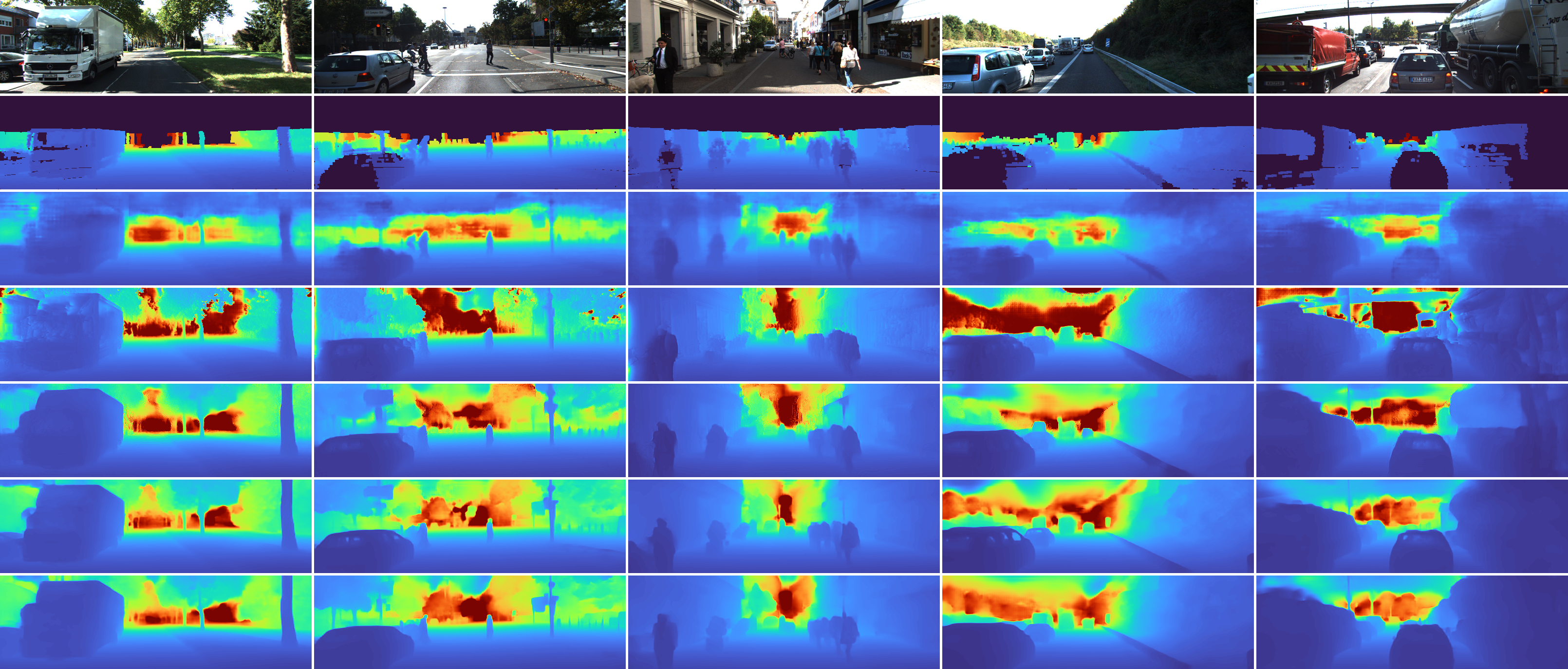
Figure 3: Qualitative results on the (KR) Eigen et al. testing slit [5]. From top to bottom: input images, their LiDAR-based depth GT (interpolated for visualization using [67]), DORN, SharinGAN, PackNet-SfM, MonoDEVSNet VK_v1 and VK_v2.

IV-D4 Qualitative results

Figure 3 presents qualitatively results relying on the depth color map commonly used in the MDE literature. We show results for representative methods in Table III, namely, DORN (LiDAR supervision), SharinGAN (stereo self-supervision and virtual-world supervision), PackNet-SfM (SfM self-supervision and ego-vehicle speed supervision), and MonoDEVSNet (Ours) using VK_v1 and VK_v2 (SfM self-supervision and virtual-world supervision). We also show the corresponding LiDAR-based GT. This GT shows that for LiDAR configurations such as the one used to acquire KITTI dataset, detecting some close vehicles may be problematic since only a few LiDAR points capture their presence. Despite being trained on LiDAR supervision, DORN provides more accurate depth information in these corner cases than the raw LiDAR, which is an example of the relevance of MDE in general. However, DORN shows worse results in these corner cases than the rest (SharinGAN/PackNet-SfM/Ours), even being more accurate in terms of MDE metrics, which focus on global assessment. SharinGAN has more difficulties than PackNet-SfM and our proposal for providing sharp borders in vertical objects/infra-structure (e.g., vehicles, pedestrians, traffic signs, trees). An interesting point to highlight is also the qualitative difference that we observe on our results depending on the use of VK version. In VK_v1 data, vehicle windows appear as transparent to depth, like in many cases happens with LiDAR data, while in VK_v2 they appear as solid. This is translated to the MDE results as we can observe comparing the two bottom rows of Fig. 3. Technically, we think the qualitative results of VK_v2 make more sense since the windows are there at the given depth. However, what we would like to highlight is that we can select one option or another thanks to the use of virtual-world data.

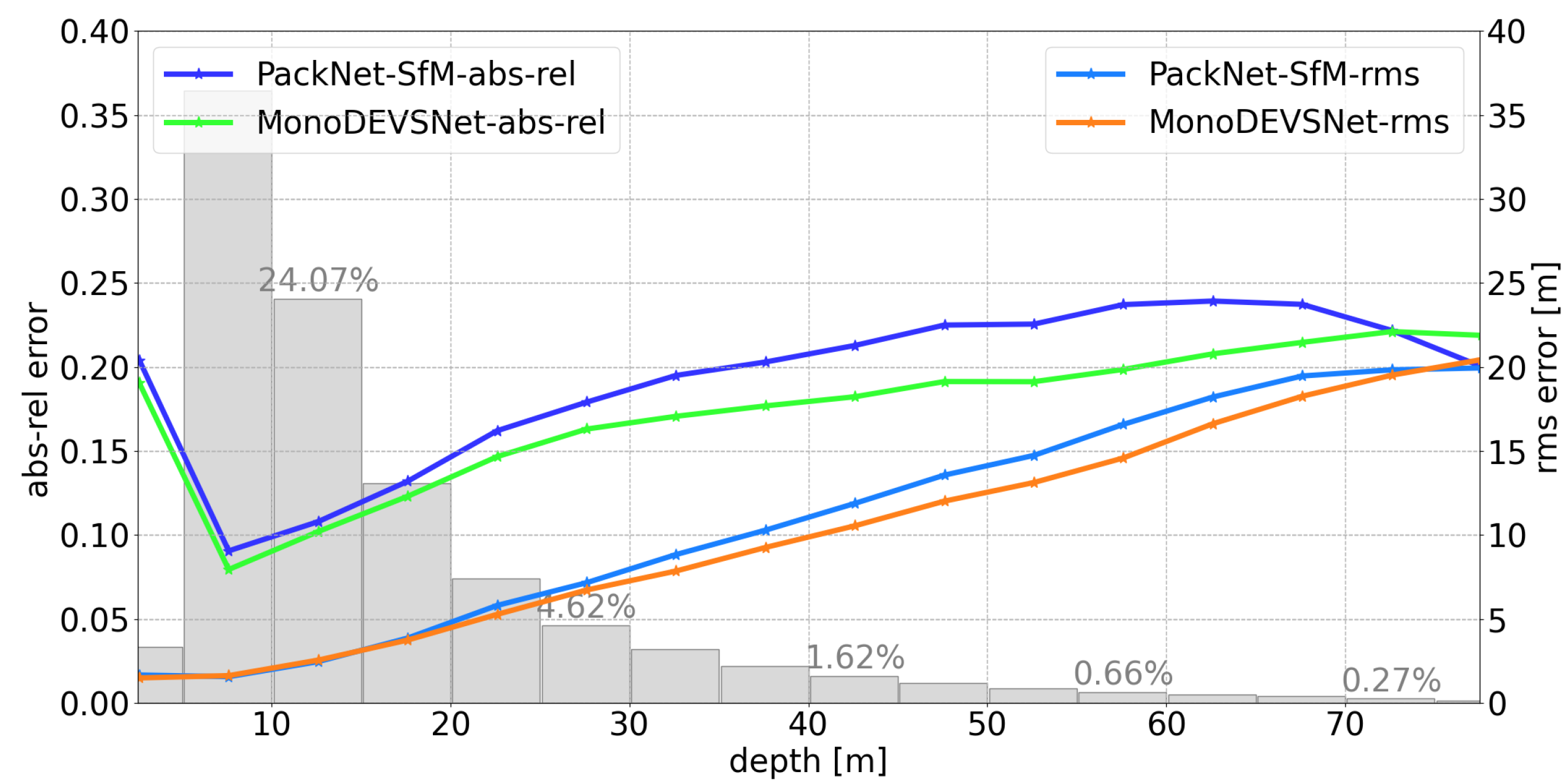
Figure 4: Abs-rel and rms errors as a function of depth, for KR Eigen testing split [5]. The histogram of depth GT is shown with bars. We compare PackNet-SfM and MonoDEVSNet.

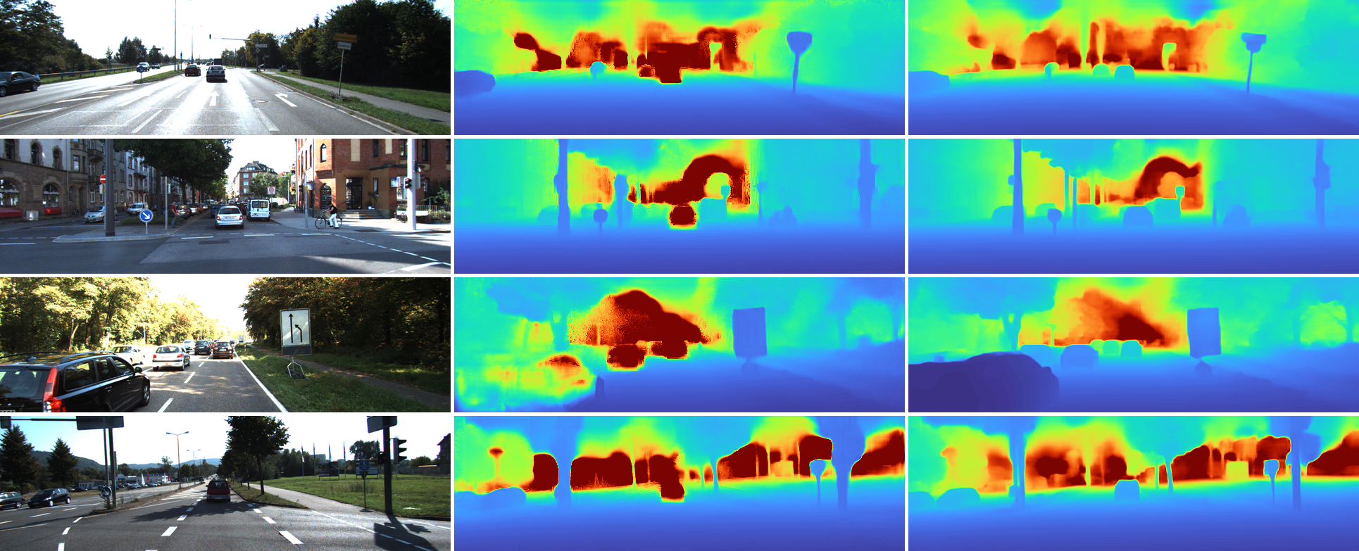
Figure 5: Qualitative results on KS data. From left to right: input images, PackNet-SfM, MonoDEVSNet.

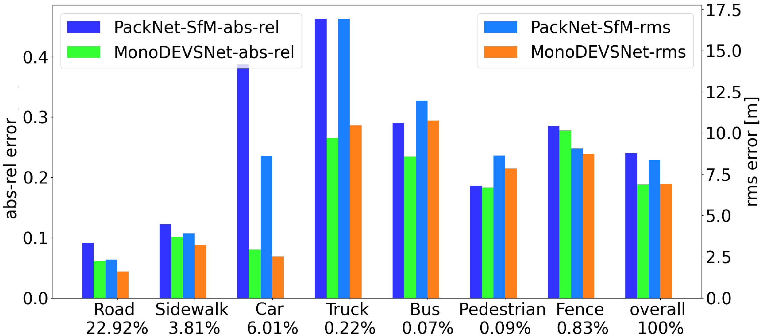
Figure 6: Per-class abs-rel and rms errors for KS, computed by averaging over the pixels of each class, for PackNet-SfM and MonoDEVSNet. The $\%$ of pixels of each class is shown.

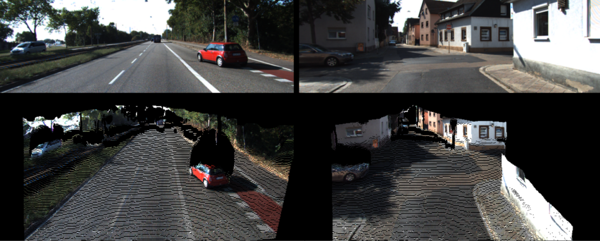
Figure 7: Point cloud representation on KR Eigen test split [5] and KS data from left to right. From top to bottom: input images, MonoDEVSNet textured point cloud.

IV-D5 Additional insights

In terms of qualitative results we think the best performing and most similar approaches are PackNet-SfM and MonoDEVSNet, both relying on real-world monocular systems. Thus, we perform a deeper comparison of them. First, following PackNet-SfM article [22], Fig. 4 plots the abs-rel error as a function of depth. Since this is a relative error, we also plot rms. Results are similar within a close range of up to $20$m. Within $20$m and $70$m, our proposal clearly outperforms PackNet-SfM and beyond $70$m both methods perform similarly. How these differences translate to abs-rel and rms global scores depends on the number of pixels falling in each distance range, which we show as an histogram in the same plot. We see how for the KR testing set most of the pixels fall in the $5-20$m depth range, where both methods perform more similarly. Second, we provide further comparative insights by using KS data since it has associated per-class semantic GT. Note that, although KS is a different data split than the one used in the experiments shown so far (KR), still is KITTI data; thus, we are not yet facing experiments about generalization. Figure 5 compares qualitative results of PackNet-SfM vs. MonoDEVSNet. We can see how PackNet-SfM misses some vehicles that our proposal does not. We believe that these vehicles may be moving at a similar speed w.r.t the ego-vehicle, which may be problematic for pure SfM-based approaches and we hypothesize that virtual-world supervision can help to avoid this problem. Figure 6 shows the corresponding abs-rel metric per-class, focusing on the most relevant classes for driving. Note how the main differences between PackNet-SfM and MonoDEVSNet are observed on vehicles, especially on cars.

Additional qualitative results are added in Fig. 7, where we can see how original images from KR and KS can be rendered as a textured point cloud. In particular, the viewpoint of these renders can change with respect to the original images thanks to the absolute depth values obtained with MonoDEVSNet.

IV-D6 Generalization results

As done in the previous literature using VK to support MDE [36, 35, 37, 38], we assess generalization on Make3D dataset. As in this literature, we follow the standard data conditioning (cropping and resizing) for models trained on KR, as well as the standard protocol introduced in [17] to compute MDE evaluation metrics (e.g. only depth below $70$m is considered). Table V presents the quantitative results usually reported for Make3D, and ours. Note how, in generalization terms, our method also outperforms the rest. Moreover, Fig. 8 shows how our proposal captures the depth structure even better than the depth GT, which is build from ${55\times 305}$ depth maps acquired by a 3D scanner. In addition, we show qualitative results on Cityscapes dataset [66] in Fig. 9. This dataset is captured in a real-world driving setup similar to car mounted videos of KITTI.

TABLE V: Absolute depth results on Make3D testing set. All the shown methods use Make3D only for testing (generalization), except (¹) which fine-tunes on Make3D training set too.

Method	abs-rel	sq-rel	rms
[35] $T^{2}$Net / VK_v1	0.508	6.589	8.935
[36] AdaDepth-S1 / VK_v1	0.452	5.71	9.559
[37] GASDA / VK_v1	0.403	6.709	10.424
[38] SharinGAN / VK_v1	0.377	4.900	8.388
MonoDEVSNet / VK_v1	0.381	3.997	7.949
MonoDEVSNet / VK_v2	0.377	3.782	8.011

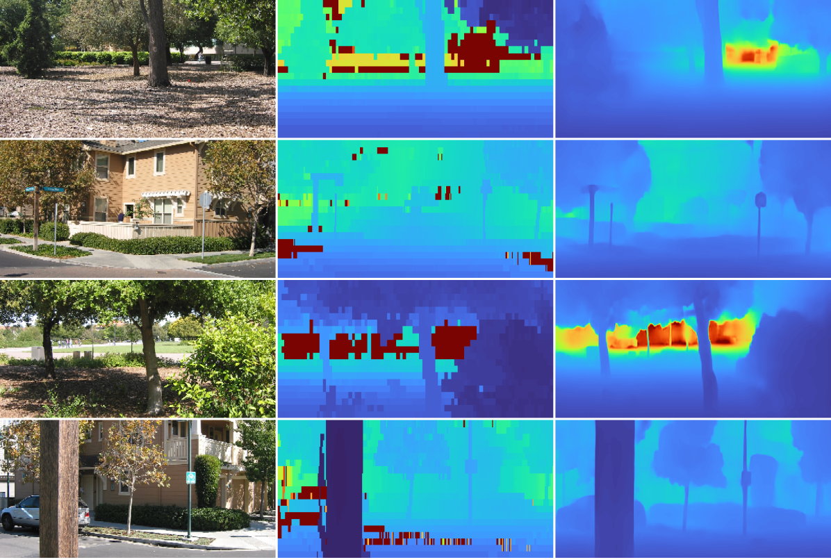
Figure 8: Qualitative results of MonoDEVSNet on Make3D. From left to right: input images, depth GT, MonoDEVSNet.

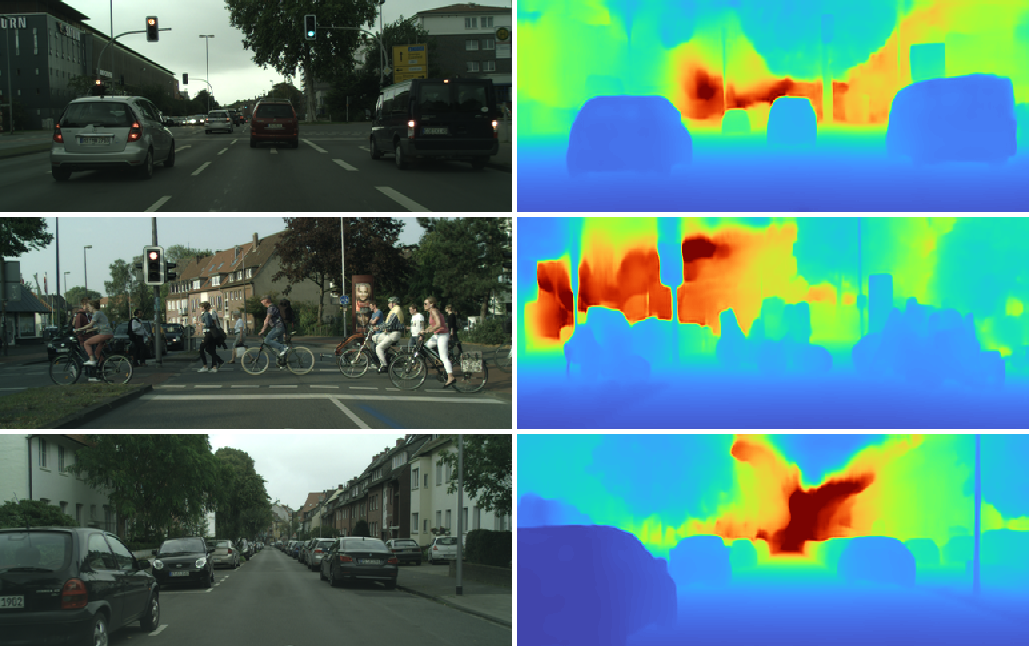
Figure 9: Qualitative results of MonoDEVSNet on Cityscapes dataset. From left to right: input images, MonoDEVSNet estimated depth maps.

IV-D7 Failure cases

Fig. 10 shows qualitative results where some errors in the depth map are highlighted: (1) overexposed pixel columns lead to hallucinate a vertical structure; (2) saturated fence segments are not seen; (3) pedestrians are visible but with an approximate silhouette; (4) a bridge is not seen; (5) saturated skies do not appear as faraway. Thinking in the information required to drive and assuming that depth estimation is combined with semantic segmentation, we think that the cases (3) and (5) are not a problem and the (2) would be only if the unseen segment is too large (which is not the case in the shown example). The case (4) could be a problem for an autonomous bus/truck provided it does not fit below the bridge, but usually those would have predefined routes where this should not happen. However, (1) can be a problem depending where the hallucinated structure appears, e.g., in the example probably it would not be a problem, but it would be if the structure appears in the middle of the road. Behind some errors, we can find the lack of training data (e.g., for the bridge not seen). Behind others, we find extreme imaging conditions (like overexposed image areas). In the former case, we need to re-train by taking these cases into account; while, in the latter case, we need to prevent such undesired effects (e.g. by using HDR camera settings). It is worth to mention that we have seen similar errors in other methods in the literature.

Figure 10: Failure cases in the depth map.

IV-D8 Revisiting $\theta^{\mbox{{\scriptsize enc}}}$ architectures

We selected HRNet-W48 because it provides the most accurate results, however, we may need to sacrifice accuracy to reduce the computational burden. Thus, we have run more experiments with the final MonoDEVS training approach, just changing $\theta^{\mbox{{\scriptsize enc}}}$. These include representative architectures of ResNet and HRNet types, as well as, DenseNet [68]. As ResNet, DenseNet does not need adding the pyramidal blocks ($\theta^{\mbox{{\scriptsize pyr}}}$). Moreover, as we mentioned in Sect. IV-A, to keep our experimental work manageable, we used 12K triplets (samples) from the real- and virtual-world training sets; however, it is possible to use $\sim\mbox{40K}$ samples from KR, which is the common practice in the literature (as those using KR in Tables I-III). Likewise, we use $\sim\mbox{22K}$ samples from VK_v2 as other literature methods in Table V do with VK_v1. Table VI presents the corresponding results. The block $\sim\mbox{40K/22K}$ can be directly compared to the literature in Table III). We see how, indeed, HRNet-W48 is the best in term of accuracy metrics. However, we see that DenseNet-121 offers the best trade-off between memory (MW) and computational (GFLOPS) requirements, offering real-time (FPS) with accuracy close to the state-of-the-art. If we need to reduce the computational burden and significantly increase the FPS, then ResNet-18 is a reasonable alternative.

TABLE VI: Absolute depth. We provide final experimental results for different versions of three different architectures. In the upper block of the table we have used the same training set as in previous experiments, i.e., 12K/12K from KR/VK_v2. In the bottom block, as is usual in the literature, we use all the available training data, i.e., $\sim\mbox{40K}$ and $\sim\mbox{22K}$, respectively.

$\theta^{\mbox{{\scriptsize enc}}}$ Backb.	MW	GFLOPS	FPS	abs-rel	sq-rel	rms	$1.25$	$1.25^{2}$
ResNet-18	11.6	4.47	141.2	0.116	0.836	4.735	0.860	0.954
ResNet-152	60.2	19.29	30.71	0.108	0.759	4.559	0.870	0.960
HRNet-W18	9.5	8.29	15.79	0.109	0.773	4.524	0.871	0.960
HRNet-W48	65.3	40.04	15.48	0.104	0.721	4.396	0.880	0.962
DenseNet-121	6.9	7.09	32.60	0.116	0.812	4.646	0.854	0.960
DenseNet-161	26.5	19.21	24.87	0.111	0.763	4.516	0.864	0.960
ResNet-18	11.6	4.47	141.2	0.114	0.838	4.734	0.860	0.954
ResNet-152	60.2	19.29	30.71	0.104	0.784	4.560	0.878	0.0.960
HRNet-W18	9.5	8.29	15.79	0.105	0.745	4.470	0.877	0.961
HRNet-W48	65.3	40.04	15.48	0.101	0.703	4.413	0.882	0.962
DenseNet-121	6.9	7.09	32.60	0.111	0.786	4.536	0.870	0.960
DenseNet-161	26.5	19.21	24.87	0.109	0.760	4.440	0.873	0.962

V Conclusion

For on-board perception, we have addressed monocular depth estimation by virtual-world supervision (MonoDEVS) and real-world SfM-inspired self-supervision; the former compensating for the inherent limitations of the latter. This challenging setting allows to rely on a monocular system not only at testing time, but also at training time; a cheap and scalable approach. We have designed a CNN, MonoDEVSNet, which seamlessly trains on real- and virtual-world data, exploiting semantic and depth supervision from the virtual-world data, and addressing the virtual-to-real domain gap by a relatively simple approach which does not add computational complexity in testing time. We have performed a comprehensive set of experiments assessing quantitative results in terms of relative and absolute depth, generalization, and we show the relevance of the components involved on MonoDEVSNet training. Our proposal yields state-of-the-art results within the SfM-based setting, even outperforming stereo-based self-supervised approaches. Qualitative results also confirm that MonoDEVSNet properly captures the depth structure of the images. As a result, we show the usefulness of leveraging virtual-world supervision to ultimately reach the upper-bound performance of methods based on LiDAR supervision. Therefore, our next steps will focus on analyzing the detailed differences between LiDAR-based supervision methods and MonoDEVSNet to find even better ways to benefit from virtual-world supervision.

-A MonoDELSNet

We introduce Monocular Depth Estimation through LiDAR Supervision and SfM Self-Supervision (MonoDELSNet) for real-world datasets, which is an adaptation of the MonoDEVSNet proposal. In MonoDELSNet we replace the virtual-world supervision of MonoDEVSNet by real-world LiDAR supervision. In addition, as for these experiments supervision and SfM self-supervision come from the same domain, we have removed the domain classifier and gradient-reversal-layer (GRL) components present in MonoDEVSNet. Furthermore, as the supervision for semantic classes is not available in this case, we do not consider the class weighting mask used to train MonoDEVSNet. The modified proposal is summarized in Fig. 11.

-A1 LiDAR Supervised loss: ${\mathcal{L}^{\mbox{{\scriptsize lsp}}}(\theta;{X^{r}.Y^{r}})}$

Since we address an estimation problem and we use depth supervision (ground truth), captured with a LiDAR sensor, we use a corresponding loss, $\mathcal{L}^{\mbox{{\scriptsize lsp}}}$, based on the L1 metric. We denote the depth supervision as $Y^{r}=\{d^{r}_{t}\}_{t=1}^{N^{r}}$, where $d^{r}_{t}$ is its depth map supervision for the corresponding frame in $X^{r}=\{x^{r}_{t}\}_{t=1}^{N^{r}}$, and $N^{r}$ is the number of frames with such supervision. Accordingly, we define the LiDAR-based loss function as:

$${\mathcal{L}^{\mbox{{\scriptsize lsp}}}(\theta;{X^{r}.Y^{r}})}=\sum_{t=1}^{N^{r}}\|{{\Psi(\theta;x^{r}_{t})}-d^{r}_{t}}\|_{1}\enspace,$$ (4)

where ${\Psi(\theta;x^{r}_{t})}$ is the estimated depth for frame $x^{r}_{t}$, being $\theta=\{\theta^{\mbox{{\scriptsize enc}}},\theta^{\mbox{{\scriptsize pyr}}},\theta^{\mbox{{\scriptsize dec}}}\}$. The SfM self-supervised loss is ${\mathcal{L}^{\mbox{{\scriptsize sf}}}(\theta,\vartheta^{\mbox{{\scriptsize sf}}};{X^{r}})}$, as defined in MonoDEVSNet.

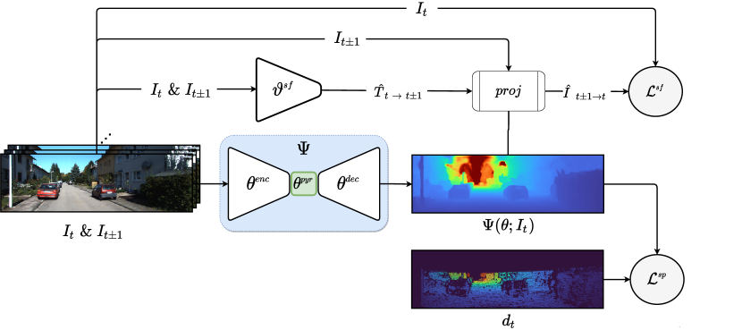
Figure 11: Training framework for MonoDELSNet, i.e., ${\Psi(\theta;x)}$ uses SfM self-supervision and LiDAR supervision. We show the involved images, GT from LiDAR, weights, and losses.

-A2 Overall training procedure

Algorithm 2 summarizes the steps to compute the needed gradient vectors for mini-batch optimization. In particular, the gradients related to MonoDELSNet’ weights, $\theta$, and those related to the auxiliary task (SfM self-supervision), i.e., $\vartheta^{\mbox{{\scriptsize sf}}}$.

Algorithm 2 Computing the gradients ${\Delta_{\theta}}$, ${\Delta_{\vartheta^{\mbox{{\scriptsize sf}}}}}$ for a mini-batch $X^{r}_{B}.Y^{r}_{B}\subset X^{r}.Y^{r}$. ${\nabla_{\xi}}F(\xi)$ refers to back-propagation on $F(\xi)$ with respect to weights $\xi$. Analogous for ${\nabla_{\xi_{i}}}F(\xi_{1},\xi_{2})$ regarding $F(\xi_{1},\xi_{2})$ and $\xi_{i}\subset\xi_{1}\cup\xi_{2}$.

Forward Passes with $\{X^{r}_{B},Y^{r}_{B}\}$

$$\ell^{\mbox{{\scriptsize lsp}}}(\theta)\leftarrow {\mathcal{L}^{\mbox{{\scriptsize lsp}}}(\theta;{X^{r}_{B}.Y^{r}_{B}})}$$

Back-propagation for Supervision

$${\Delta^{\mbox{{\scriptsize lsp}}}_{\theta}}\leftarrow {\nabla_{\theta}}\ell^{\mbox{{\scriptsize lsp}}}(\theta)$$

Forward Passes with $X^{r}_{B}$

$$\ell^{\mbox{{\scriptsize sf}}}(\theta,\vartheta^{\mbox{{\scriptsize sf}}})\leftarrow {\mathcal{L}^{\mbox{{\scriptsize sf}}}(\theta,\vartheta^{\mbox{{\scriptsize sf}}};X^{r}_{B})}$$

Back-propagation for Self-supervision

$${\Delta^{\mbox{{\scriptsize sf}}}_{\theta}}\leftarrow {\nabla_{\theta}}\ell^{\mbox{{\scriptsize sf}}}(\theta,\vartheta^{\mbox{{\scriptsize sf}}})$$

Setting the final gradient vectors

$${\Delta_{\vartheta^{\mbox{{\scriptsize sf}}}}}\leftarrow {\nabla_{\vartheta^{\mbox{{\scriptsize sf}}}}}\ell^{\mbox{{\scriptsize sf}}}(\theta,\vartheta^{\mbox{{\scriptsize sf}}})$$

$$\omega^{\mbox{{\scriptsize sf}}}\leftarrow \ell^{\mbox{{\scriptsize lsp}}}(\theta)/\ell^{\mbox{{\scriptsize sf}}}(\theta,\vartheta^{\mbox{{\scriptsize sf}}})$$

$${\Delta_{\theta}}\leftarrow {\Delta^{\mbox{{\scriptsize lsp}}}_{\theta}}+\omega^{\mbox{{\scriptsize sf}}}{\Delta^{\mbox{{\scriptsize sf}}}_{\theta}}$$

-A3 Experimental results

Dataset and Training details

For training MonoDELSNet, we use the popular KITTI Raw (KR) dataset. Here, we follow Zhou et al. [19] training-testing split. From the training split, we select  40K monocular triplets, i.e., samples of the form $\{x^{r}_{t-1},x^{r}_{t},x^{r}_{t+1}\}$, as well as an isolated sample of each triplet, $\{x^{r}_{t}\}$, with densified LiDAR-based depth ground truth $\{d^{r}_{t}\}$. The former for providing SfM self-supervision, the latter for providing LiDAR supervision. For evaluation purposes, among the testing split (697 images) introduced by Eigen et al. [5], we considered the 652 isolated images with densified LiDAR-based depth supervision, i.e., as is common practice in the state-of-the-art methods on monocular depth estimation. HRNet-w48 [62] is used as backbone encoder, where its weights are initialized with ImageNet [65] weights. Furthermore, the input images are processed at their original resolution, i.e., ${\sim 1248\times 384}$ pix.

Results and discussion

We compare our method with LiDAR supervision methods such as VNL [14] , DORN [10], DPT [69], AdaBins [70] and with our combination of virtual-world supervision and SfM self-supervision, i.e., MonoDEVSNet. VNL combines supervision with 3D geometric constraints to improve the depth estimation accuracy. AdaBins proposes to learn adaptive bins per image. Similar to DORN, the idea is to discretize the depth range by dividing it into N bins and estimating the probability of bins per pixel. DPT uses a transformer-based backbone architecture to learn high-resolution representations.

Again, we evaluate monocular depth estimation using the metrics proposed by Eigen et al. [5]. Table VII shows our quantitative results compared to others of the state-of-the-art. Note how MonoDELSNet outperforms them. Fig. 12 presents qualitatively results using a standard depth colormap. For completeness, we run experiments for MonoDEVSNet and MonoDELSNet based on the widely used resolution of $640\times 192$ pix. Thanks to the LiDAR supervision, MonoDELSNet performs better. In addition, for the resolution of $1248\times 384$ pix., we run MonoDELSNet with two different encoders, namely, ResNet-18 (also initialized from ImageNet for training) and HRNet-w48. The latter outperforms the former. We also assessed the results when the LiDAR supervision is used, but not the SfM-based self-supervision. We see that adding SfM-based self-supervision improves the results.

TABLE VII: Absolute depth results up to $80$m (see main text for details). ${(^{1})}$ stands for models trained at the standard resolution $640\times 192$ pix. ${(^{2})}$ indicates the use of ResNet-18 instead of HRNet-w48 as encoder. ${(^{3})}$ using LiDAR supervision only.

Method	abs-rel	sq-rel	rms	rms-log	$1.25$	$1.25^{2}$	$1.25^{3}$
[14] VNL	0.072	N/A	3.258	0.117	0.932	0.984	0.994
[10] DORN	0.072	N/A	2.626	0.120	0.932	0.984	0.994
[69] DPT	0.062	0.222	2.573	0.092	0.959	0.995	0.999
[70] AdaBins	0.058	0.190	2.360	0.088	0.964	0.995	0.999
MonoDEVSNet1	0.073	0.298	2.802	0.108	0.939	0.990	0.988
MonoDELSNet1	0.065	0.281	2.951	0.102	0.948	0.992	0.998
MonoDELSNet2	0.062	0.217	2.502	0.097	0.954	0.994	0.998
MonoDELSNet	0.053	0.161	2.101	0.082	0.969	0.996	0.999
MonoDELSNet3	0.057	0.217	2.613	0.092	0.960	0.994	0.998

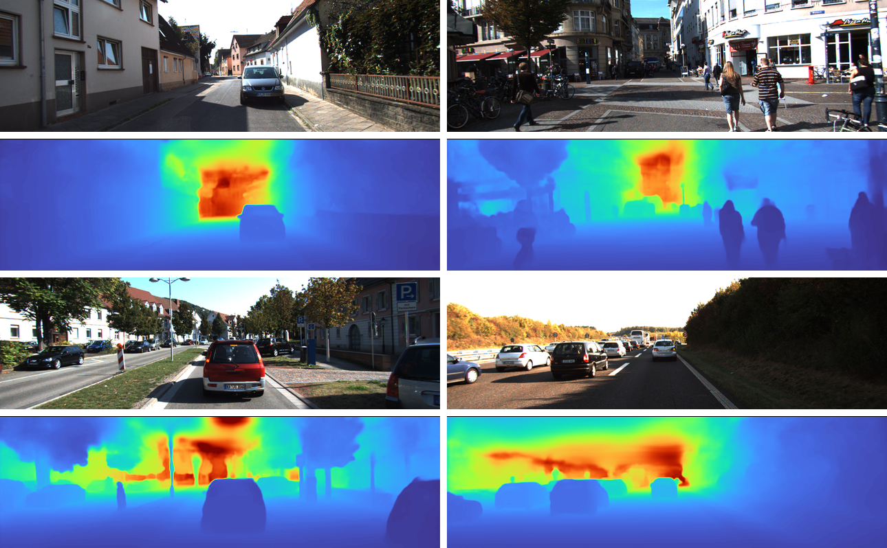
Figure 12: Qualitative results on the KR Eigen et al. testing split. From top to bottom, twice: input RGB image, and MonoDELSNet estimated depth maps.

-A4 Conclusion

our MonoDEVNet framework can be adapted to work with LiDAR supervision and SfM self-supervision. This approach, here named as MonoDELSNet, reports state-of-the-art results on monocular depth estimation.

-A5 Publicly available code

The MonoDELSNet is part of the MonoDEVSNet framework, thus, it can be found also here: https://github.com/HMRC-AEL/MonoDEVSNet

References

- [1] S. Dokhanchi, B. Mysore, K. Mishra, and B. Ottersten, “Enhanced automotive target detection through RADAR and communications sensor fusion,” in Int. Conf. on Acoustics, Speech, and Signal Processing (ICASSP), 2021.
- [2] Y. Zhou and O. Tuzel, “VoxelNet: End-to-end learning for point cloud based 3D object detection,” in Int. Conf. on Computer Vision and Pattern Recognition (CVPR), 2018.
- [3] S. Deac, I. Giosan, and S. Nedevschi, “Curb detection in urban traffic scenarios using lidars point cloud and semantically segmented color images,” in Intelligent Transportation Systems Conference (ITSC), 2019.
- [4] X. Cheng, Y. Zhong, M. Harandi, Y. Dai, X. Chang, T. Drummond, H. Li, and Z. Ge, “Hierarchical neural architecture search for deep stereo matching,” in Neural Information Processing Systems (NeurIPS), 2020.
- [5] D. Eigen, C. Puhrsch, and R. Fergus, “Depth map prediction from a single image using a multi-scale deep network,” in Neural Information Processing Systems (NeurIPS), 2014.
- [6] F. Liu, C. Shen, G. Lin, and I. Reid, “Learning depth from single monocular images using deep convolutional neural fields,” IEEE Trans. on Pattern Analysis and Machine Intelligence, vol. 38, no. 10, pp. 2024–2039, 2016.
- [7] A. Roy and S. Todorovic, “Monocular depth estimation using neural regression forest,” in Int. Conf. on Computer Vision and Pattern Recognition (CVPR), 2016.
- [8] I. Laina, C. Rupprecht, V. Belagiannis, F. Tombari, and N. Navab, “Deeper depth prediction with fully convolutional residual networks,” in Int. Conf. on 3D Vision (3DV), 2016.
- [9] Y. Cao, Z. Wu, and C. Shen, “Estimating depth from monocular images as classification using deep fully convolutional residual networks,” IEEE Trans. on Circuits and Systems for Video Technology, 2017.
- [10] H. Fu, M. Gong, C. Wang, K. Batmanghelich, and D. Tao, “Deep ordinal regression network for monocular depth estimation,” in Int. Conf. on Computer Vision and Pattern Recognition (CVPR), 2018.
- [11] A. Gurram, O. Urfalioglu, I. Halfaoui, F. Bouzaraa, and A. López, “Monocular depth estimation by learning from heterogeneous datasets,” in Intelligent Vehicles Symposium (IV), 2018.
- [12] L. He, G. Wang, and Z. Hu, “Learning depth from single images with deep neural network embedding focal length,” IEEE Trans. on Image Processing, vol. 27, no. 9, pp. 4676–4689, 2018.
- [13] D. Xu, W. Wang, H. Tang, H. Liu, N. Sebe, and E. Ricci, “Structured attention guided convolutional neural fields for monocular depth estimation,” in Int. Conf. on Computer Vision and Pattern Recognition (CVPR), 2018.
- [14] W. Yin, Y. Liu, C. Shen, and Y. Yan, “Enforcing geometric constraints of virtual normal for depth prediction,” in International Conference on Computer Vision (ICCV), 2019.
- [15] A. Saxena, J. Schulte, and A. Ng, “Depth estimation using monocular and stereo cues,” in Int. Joint Conf. on Artificial Intelligence, 2007.
- [16] R. Garg, V. Kumar, G. Carneiro, and I. Reid, “Unsupervised cnn for single view depth estimation: Geometry to the rescue,” in European Conference on Computer Vision (ECCV), 2016.
- [17] C. Godard, O. Aodha, and G. Brostow, “Unsupervised monocular depth estimation with left-right consistency,” in Int. Conf. on Computer Vision and Pattern Recognition (CVPR), 2017.
- [18] S. Pillai, R. Ambruş, and A. Gaidon, “SuperDepth: Self-supervised, super-resolved monocular depth estimation,” in Int. Conf. on Robotics and Automation (ICRA), 2019.
- [19] T. Zhou, M. Brown, N. Snavely, and D. Lowe, “Unsupervised learning of depth and ego-motion from video,” in Int. Conf. on Computer Vision and Pattern Recognition (CVPR), 2017.
- [20] Z. Yin and J. Shi, “GeoNet: Unsupervised learning of dense depth, optical flow and camera pose,” in Int. Conf. on Computer Vision and Pattern Recognition (CVPR), 2018.
- [21] W. Zhao, S. Liu, Y. Shu, and Y.-J. Liu, “Towards better generalization: Joint depth-pose learning without PoseNet,” in Int. Conf. on Computer Vision and Pattern Recognition (CVPR), 2020.
- [22] V. Guizilini, R. Ambrus, S. Pillai, A. Raventos, and A. Gaidon, “3D packing for self-supervised monocular depth estimation,” in Int. Conf. on Computer Vision and Pattern Recognition (CVPR), 2020.
- [23] C. Godard, O. Mac Aodha, M. Firman, and G. J. Brostow, “Digging into self-supervised monocular depth estimation,” in International Conference on Computer Vision (ICCV), 2019.
- [24] Y. Kuznietsov, J. Stückler, and B. Leibe, “Semi-supervised deep learning for monocular depth map prediction,” in Int. Conf. on Computer Vision and Pattern Recognition (CVPR), 2017.
- [25] L. He, C. Chen, T. Zhang, H. Zhu, and S. Wan, “Wearable depth camera: Monocular depth estimation via sparse optimization under weak supervision,” IEEE Accesss, vol. 6, pp. 41 337–41 345, 2018.
- [26] V. Guizilini, J. Li, R. Ambrus, S. Pillai, and A. Gaidon, “Robust semi-supervised monocular depth estimation with reprojected distances,” in Conference on Robot Learning (CoRL), 2020.
- [27] R. de Queiroz Mendes, E. G. Ribeiro, N. dos Santos Rosa, and V. Grassi Jr, “On deep learning techniques to boost monocular depth estimation for autonomous navigation,” Robotics and Autonomous Systems, vol. 136, p. 103701, February 2021.
- [28] A. Gaidon, Q. Wang, Y. Cabon, and E. Vig, “Virtual worlds as proxy for multi-object tracking analysis,” in Int. Conf. on Computer Vision and Pattern Recognition (CVPR), 2016.
- [29] Y. Cabon, N. Murray, and M. Humenberger, “Virtual KITTI 2,” arXiv:2001.10773, 2020.
- [30] G. Ros, L. Sellart, J. Materzyska, D. Vázquez, and A. López, “The SYNTHIA dataset: a large collection of synthetic images for semantic segmentation of urban scenes,” in Int. Conf. on Computer Vision and Pattern Recognition (CVPR), 2016.
- [31] N. Mayer, E. Ilg, P. Hausser, P. Fischer, D. Cremers, A. Dosovitskiy, and T. Brox, “A large dataset to train convolutional networks for disparity, optical flow, and scene flow estimation,” in Int. Conf. on Computer Vision and Pattern Recognition (CVPR), 2016.
- [32] S. R. Richter, Z. Hayder, and V. Koltun, “Playing for benchmarks,” in International Conference on Computer Vision (ICCV), 2017.
- [33] S. Shah, D. Dey, C. Lovett, and A. Kapoor, “AirSim: High-fidelity visual and physical simulation for autonomous vehicles,” in Int. Conf. on Field and Service Robotics (FSR), 2017.
- [34] A. Dosovitskiy, G. Ros, F. Codevilla, A. López, and V. Koltun, “CARLA: An open urban driving simulator,” in Conference on Robot Learning (CoRL), 2017.
- [35] C. Zheng, T.-J. Cham, and J. Cai, “T2Net: Synthetic-to-realistic translation for solving single-image depth estimation tasks,” in European Conference on Computer Vision (ECCV), 2018.
- [36] J. Nath Kundu, P. Krishna Uppala, A. Pahuja, and R. Venkatesh Babu, “AdaDepth: Unsupervised content congruent adaptation for depth estimation,” in Int. Conf. on Computer Vision and Pattern Recognition (CVPR), 2018.
- [37] S. Zhao, H. Fu, M. Gong, and D. Tao, “Geometry-aware symmetric domain adaptation for monocular depth estimation,” in Int. Conf. on Computer Vision and Pattern Recognition (CVPR), 2019.
- [38] K. PNVR, H. Zhou, and D. Jacobs, “SharinGAN: Combining synthetic and real data for unsupervised geometry estimation,” in Int. Conf. on Computer Vision and Pattern Recognition (CVPR), 2020.
- [39] B. Cheng, I. S. Saggu, R. Shah, G. Bansal, and D. Bharadia, “S3Net: Semantic-aware self-supervised depth estimation with monocular videos and synthetic data,” in European Conference on Computer Vision (ECCV), 2020.
- [40] G. Csurka, A Comprehensive Survey on Domain Adaptation for Visual Applications, ser. Advances in Computer Vision and Pattern Recognition. Springer, 2017, ch. 1.
- [41] M. Wang and W. Deng, “Deep visual domain adaptation: A survey,” Neurocomputing, vol. 312, pp. 135–153, October 2018.
- [42] G. Wilson and D. Cook, “A survey of unsupervised deep domain adaptation,” ACM Transactions on Intelligent Systems and Technology, vol. 11, no. 5, 2020.
- [43] Y. Ganin and V. Lempitsky, “Unsupervised domain adaptation by backpropagation,” in Int. Conf. on Machine Learning (ICML), 2015.
- [44] Y. Ganin, E. Ustinova, H. Ajakan, P. Germain, H. Larochelle, F. Laviolette, M. Marchand, and V. Lempitsky, “Domain-adversarial training of neural networks,” The Journal of Machine Learning Research, vol. 17, no. 1, pp. 2096–2030, 2016.
- [45] B. Liu, S. Gould, and D. Koller, “Single image depth estimation from predicted semantic labels,” in Int. Conf. on Computer Vision and Pattern Recognition (CVPR), 2010.
- [46] L. Ladicky, J. Shi, and M. Pollefeys, “Pulling things out of perspective,” in Int. Conf. on Computer Vision and Pattern Recognition (CVPR), 2014.
- [47] V. Srikakulapu, H. Kumar, S. Gupta, and K. S. Venkatesh, “Depth estimation from single image using defocus and texture cues,” in National Conference on Computer Vision, Pattern Recognition, Image Processing and Graphics (NCVPRIPG), 2015.
- [48] A. Mousavian, H. Pirsiavash, and J. Košecká, “Joint semantic segmentation and depth estimation with deep convolutional networks,” in Int. Conf. on 3D Vision (3DV), 2016.
- [49] O. Jafari, O. Groth, A. Kirillov, M. Yang, and C. Rother, “Analyzing modular CNN architectures for joint depth prediction and semantic segmentation,” in Int. Conf. on Robotics and Automation (ICRA), 2017.
- [50] J. Jiao, Y. Cao, Y. Song, and R. Lau, “Look deeper into depth: Monocular depth estimation with semantic booster and attention-driven loss,” in European Conference on Computer Vision (ECCV), 2018.
- [51] V. Guizilini, R. Hou, J. Li, R. Ambrus, and A. Gaidon, “Semantically-guided representation learning for self-supervised monocular depth,” in Int. Conf. on Learning Representation (ICLR), 2020.
- [52] P.-Y. Chen, A. H. Liu, Y.-C. Liu, and Y.-C. F. Wang, “Towards scene understanding: Unsupervised monocular depth estimation with semantic-aware representation,” in Int. Conf. on Computer Vision and Pattern Recognition (CVPR), 2019.
- [53] O. Özyeşil, V. Voroninski, R. Basri, and A. Singer, “A survey of structure from motion,” Acta Numerica, vol. 26, pp. 305–364, 1st May 2017.
- [54] Z. Wang, A. C. Bovik, H. R. Sheikh, and E. P. Simoncelli, “Image quality assessment: from error visibility to structural similarity,” IEEE Trans. on Image Processing, vol. 13, no. 4, pp. 600–612, 2004.
- [55] I. Goodfellow, J. Pouget-Abadie, M. Mirza, B. Xu, D. Warde-Farley, S. Ozair, A. Courville, and Y. Bengio, “Generative adversarial nets,” in Neural Information Processing Systems (NeurIPS), 2014.
- [56] Y. Choi, Y. Uh, J. Yoo, and J.-W. Ha, “StarGAN v2: Diverse image synthesis for multiple domains,” in Int. Conf. on Computer Vision and Pattern Recognition (CVPR), 2020.
- [57] J.-Y. Zhu, T. Park, P. Isola, and A. A. Efros, “Unpaired image-to-image translation using cycle-consistent adversarial networks,” in International Conference on Computer Vision (ICCV), 2017.
- [58] Z. Chen, V. Badrinarayanan, C.-Y. Lee, and A. Rabinovich, “GradNorm: Gradient normalization for adaptive loss balancing in deep multitask networks,” in Int. Conf. on Machine Learning (ICML), 2018.
- [59] A. Geiger, P. Lenz, C. Stiller, and R. Urtasun, “Vision meets robotics: The KITTI dataset,” International Journal of Robotics Research, vol. 32, no. 11, pp. 1231–1237, 2013.
- [60] M. Menze and A. Geiger, “Object scene flow for autonomous vehicle,” in Int. Conf. on Computer Vision and Pattern Recognition (CVPR), 2015.
- [61] A. Saxena, M. Sun, and A. Ng., “Make3D: Learning 3D scene structure from a single still image,” IEEE Trans. on Pattern Analysis and Machine Intelligence, vol. 31, no. 5, pp. 824–840, 2009.
- [62] J. Wang, K. Sun, T. Cheng, B. Jiang, C. Deng, Y. Zhao, D. Liu, Y. Mu, M. Tan, X. Wang, W. Liu, and B. Xiao, “Deep high-resolution representation learning for visual recognition,” IEEE Trans. on Pattern Analysis and Machine Intelligence, April 2020.
- [63] A. Paszke, S. Gross, F. Massa, A. Lerer, J. Bradbury, G. Chanan, T. Killeen, Z. Lin, N. Gimelshein, L. Antiga, A. Desmaison, A. Kopf, E. Yang, Z. DeVito, M. Raison, A. Tejani, S. Chilamkurthy, B. Steiner, L. Fang, J. Bai, and S. Chintala, “PyTorch: An imperative style, high-performance deep learning library,” in Neural Information Processing Systems (NeurIPS), 2019.
- [64] D. Kingma and J. Ba, “Adam : A method for stochastic optimization,” in Int. Conf. on Learning Representation (ICLR), 2015.
- [65] J. Deng, W. Dong, R. Socher, L.-J. Li, K. Li, and L. Fei-Fei, “ImageNet: A large-scale hierarchical image database,” in Int. Conf. on Computer Vision and Pattern Recognition (CVPR), 2009.
- [66] M. Cordts, M. Omran, S. Ramos, T. Rehfeld, M. Enzweiler, R. Benenson, U. Franke, S. Roth, and B. Schiele, “The Cityscapes dataset for semantic urban scene understanding,” in Int. Conf. on Computer Vision and Pattern Recognition (CVPR), 2016.
- [67] C. Premebida, J. Carreira, J. Batista, and U. Nunes, “Pedestrian detection combining RGB and dense LiDAR data,” in Int. Conf. on Intelligent Robots and Systems (IROS), 2014.
- [68] G. Huang, Z. Liu, G. Pleiss, L. Van Der Maaten, and K. Weinberger, “Convolutional networks with dense connectivity,” IEEE Trans. on Pattern Analysis and Machine Intelligence, May 2019.
- [69] R. Ranftl, A. Bochkovskiy, and V. Koltun, “Vision transformers for dense prediction,” in Int. Conf. on Computer Vision and Pattern Recognition (CVPR), 2021.
- [70] S. F. Bhat, I. Alhashim, and P. Wonka, “Adabins: Depth estimation using adaptive bins,” in Int. Conf. on Computer Vision and Pattern Recognition (CVPR), 2021.