On the nonlinear Dirichlet-Neumann method and preconditioner for Newton’s method

1 Introduction

We consider a nonlinear Partial Differential Equation (PDE)

$$\mathcal{L}(u)=f\quad\text{in}\quad\Omega,\quad u=g\quad\text{on }\partial\Omega,$$ (1)

where $\Omega\subset\mathbb{R}^{d}$ for $d\in\left\{1,2,3\right\}$ is an open bounded domain with a polygonal boundary $\partial\Omega$, and $f,g\in L^{2}(\Omega)$. We suppose that (1) admits a unique weak solution in some Hilbert space $u\in\mathcal{X}$( e.g. $H^{1}(\Omega))$. For instance, for a quasilinear operator $\mathcal{L}$ in divergence form, explicit assumptions can be found in kumbhar_p_mini_17_cai_dryja_1994 and references therein, see also (kumbhar_p_mini_17_evans2010partial, , Chapter 8-9) and (kumbhar_p_mini_17_Ciarlet, , Chapter 9). Let us divide $\Omega$ into two nonoverlapping subdomains $\Omega_{1}$ and $\Omega_{2}$ and define $\Gamma_{j}=\partial\Omega_{j}\setminus\partial\Omega$, $j=1,2$. Let $u_{j}$ be the restriction of $u$ to $\Omega_{j}$. The nonlinear Dirichlet-Neumann (DN) method starts from an initial guess $\lambda^{0}$ and computes for $n\geq 1$ until convergence

$$\begin{array}[]{l l l l l}\mathcal{L}(u_{1}^{n})&=f_{1},\quad\text{in}\quad\Omega_{1},&&\quad\mathcal{L}(u_{2}^{n})&=f_{2},\quad\text{in}\quad\Omega_{2}\\ u^{n}_{1}&=g_{1},\quad\text{on}\quad\partial\Omega_{1}\setminus\Gamma,&&\quad u^{n}_{2}&=g_{2},\quad\text{on}\quad\partial\Omega_{2}\setminus\Gamma\\ u^{n}_{1}&=\lambda^{n}\quad\text{on}\quad\Gamma,&&\quad\mathcal{N}_{2}u^{n}_{2}&=-\mathcal{N}_{1}u^{n}_{1}\quad\text{on}\quad\Gamma,\end{array}$$ (2)

where $\lambda^{n}=(1-\theta)\lambda^{n-1}+\theta u^{n-1}_{2|\Gamma},$ with $\theta\in(0,1)$ , $f_{j}:=f|_{\Omega_{j}}$ and $g_{j}:=g|_{\partial\Omega_{j}\setminus\Gamma}$ for $j=1,2$. The operators $\mathcal{N}_{j}$ represent the outward nonlinear Neumann conditions that must be imposed on the interface $\Gamma$ and are usually found through integration by parts of the variational formulation of the PDE. For instance, if $\mathcal{L}(u)=-\partial_{x}((1+\alpha u^{2})\partial_{x}u)$, then $\mathcal{N}_{j}u=(-1)^{j+1}(1+\alpha u_{|\Gamma}^{2})\partial_{x}u_{|\Gamma}$. For the well-posedness of the Dirichlet-Neumann method, we further assume that $\mathcal{N}_{j}u$ defines a bounded linear functional over $\mathcal{X}$.

System (2) can be formulated as an iteration over the substructured variable $\lambda$ as

$$\lambda^{n}=G(\lambda^{n-1}):=(1-\theta)\lambda^{n-1}+\theta\text{NtD}_{2}\left(-\text{DtN}_{1}\left(\lambda^{n-1},\psi_{1}\right),\psi_{2}\right),$$ (3)

where $\psi_{j}=(f_{j},g_{j})$, $j=1,2$, represent the force term and boundary conditions, while the nonlinear Dirichlet-to-Neumann ($\text{DtN}_{j}$) and Neumann-to-Dirichlet operators ($\text{NtD}_{j}$) are defined as $\text{DtN}_{j}(\lambda,\psi_{j}):=\mathcal{N}_{j}u_{j}$, and $\text{NtD}_{j}(\phi,\psi_{j}):=v_{j}|_{\Gamma}$, with

$$\begin{array}[]{rcllrcll}\mathcal{L}(u_{j})&=&f_{j}&\text{in $\Omega_{j}$},&\mathcal{L}(v_{j})&=&f_{j}&\text{in $\Omega_{j}$},\\ u_{j}&=&g_{j}&\text{on $\partial\Omega_{j}\setminus\Gamma$},&v_{j}&=&g_{j}&\text{on $\partial\Omega_{j}\setminus\Gamma$},\\ u_{j}&=&\lambda&\text{on $\Gamma$}&\mathcal{N}_{j}v_{j}&=&\phi&\text{on $\Gamma$}.\end{array}$$ (4)

If $u_{\text{ex}}\in H^{1}(\Omega)$ is the solution of (1), then it must have continuous Dirichlet trace and Neumann flux along the interface $\Gamma$. Defining $u_{\Gamma}:=u_{\text{ex}}|_{\Gamma}$, $\phi:=\mathcal{N}_{1}u_{\text{ex}}|_{\Gamma}$ and using the operators $\text{DtN}_{j}$ and $\text{NtD}_{j}$, these necessary properties are equivalent to

$$\text{DtN}_{1}(u_{\Gamma},\psi_{1})=-\text{DtN}_{2}(u_{\Gamma},\psi_{2}),\quad\text{and}\quad\text{NtD}_{1}(\phi,\psi_{1})=\text{NtD}_{2}(-\phi,\psi_{2}).$$ (5)

2 Nilpotent property and quadratic convergence

It is well known, see e.g. kumbhar_p_mini_17_quarteroni1999domain ; kumbhar_p_mini_17_bookCG , that if $\mathcal{L}$ is linear and the subdomain decomposition is symmetric, then the DN method converges in one iteration for $\theta=1/2$. Indeed, if $\mathcal{L}$ is linear, one can work on the error equation, i.e. $\psi_{j}=0$, and the symmetry of the decomposition is sufficient to guarantee $\text{DtN}_{1}(\cdot,0)\equiv\text{DtN}_{2}(\cdot,0)$, so that

$$\lambda^{1} =\frac{1}{2}\left(\lambda^{0}+\text{NtD}_{2}\left(-\text{DtN}_{1}(\lambda^{0},0)\right),0\right)=\frac{1}{2}\left(\lambda^{0}+\text{NtD}_{2}\left(-\text{DtN}_{2}(\lambda^{0},0)\right),0\right)$$ (6)

$$=\frac{1}{2}(\lambda^{0}-\text{NtD}_{2}(\text{DtN}_{2}(\lambda^{0},0),0)=0,$$

where in the third equality we used linearity, and in the last $\text{NtD}_{2}(\text{DtN}_{2}(\lambda,\psi),\psi)=\lambda$. Can the nonlinear DN method also converge in one iteration?

On the one hand, the relation $\text{NtD}_{j}(\text{DtN}_{j}(\lambda,\psi),\psi)=\lambda$ holds even in the nonlinear case, simply because the nonlinear $\text{DtN}_{j}$ operator is the inverse of the nonlinear $\text{NtD}_{j}$ operator. On the other hand, due to the nonlinearity of $\mathcal{L}$, one cannot rely on the error equation, cannot state that $\text{NtD}_{2}(-\phi)=-\text{NtD}_{2}(\phi)$, and the symmetry of the decomposition is not sufficient to guarantee $\text{DtN}_{1}(\lambda,\psi_{1})\equiv\text{DtN}_{2}(\lambda,\psi_{2})$, because of the boundary conditions and the force term.

A straight forward observation is that if the nonlinear DN method converges in one iteration, then $G(\lambda)=\lambda_{\text{ex}}$, $\forall\lambda$, that is $G(\cdot)$ is a constant. A necessary and sufficient condition for the nonlinear DN method to converge in one iteration is then

$$0\!=\!G^{\prime}(\lambda)\!=\!\frac{1}{2}+\frac{1}{2}\!\left(\text{NtD}_{2}\left(-\text{DtN}_{1}(\lambda,\psi_{1}),\psi_{2}\right)\right)^{\prime}\!\implies\!\left(\text{NtD}_{2}\!\left(-\text{DtN}_{1}(\lambda,\psi_{1}),\psi_{2}\right)\right)^{\prime}\!=\!-1.$$ (7)

Clearly, (7) is satisfied if $\text{NtD}_{2}(-\text{DtN}_{1}(\lambda,\psi_{1}),\psi_{2})=-\lambda$. We consider a toy example in which this condition is satisfied. Let $\mathcal{L}=-\partial_{x}\left((1+u^{2})\partial_{x}u\right)$, $u(0)=g\in\mathbb{R}^{+}$, $u(1)=-g$ and $f(x)=\sin((2k)\pi x)$. On the left plot of Fig. 1,

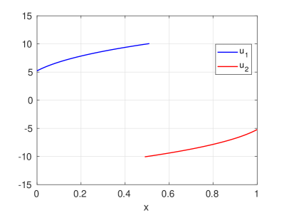
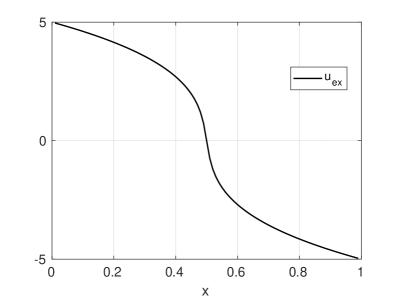
Figure 1: Subdomain solutions of the nonlinear DN method after one iteration (left), and exact solution (right). The parameters are $g=5$ and $k=2$.

we show the subdomain solutions $u_{1}$ and $u_{2}$ obtained from (2) after the first iteration. The two contributions sum to zero, which is the value of $\lambda_{\text{ex}}$. Thus, after one iteration we obtain the exact solution shown in the right panel.

Even though the nilpotent property does not hold in general, we show in the following Theorem that the nonlinear DN method can exhibit quadratic convergence.

Theorem 2.1 (Quadratic convergence of nonlinear DN)

For any one-dimensional nonlinear problem $\mathcal{L}(u)=f$ such that $\text{DtN}_{1}^{\prime}(\lambda_{\text{ex}},\psi_{1})\cdot\text{DtN}_{2}^{\prime}(\lambda_{\text{ex}},\psi_{2})>0$ with $\lambda_{\text{ex}}:=u_{\text{ex}}|_{\Gamma}$, there exists a $\theta\in(0,1)$ such that the nonlinear Dirichlet-Neumann method converges quadratically.

Proof

A sufficient condition for quadratic convergence is that the Jacobian of $G(\cdot)$, defined in (3), is zero at $\lambda_{\text{ex}}:=u_{\text{ex}}|_{\Gamma}$, that is $G^{\prime}(\lambda_{\text{ex}})=0$. A direct calculation shows

$$G^{\prime}(\lambda)=(1-\theta)+\theta\text{NtD}_{2}^{\prime}\left(-\text{DtN}_{1}(\lambda,\psi_{1}),\psi_{2}\right)\cdot\left(-\text{DtN}_{1}^{\prime}(\lambda,\psi_{1})\right).$$ (8)

Setting $\lambda=\lambda_{\text{ex}}$ and using the optimality condition $\text{DtN}_{1}(\lambda_{\text{ex}},\psi_{1})=-\text{DtN}_{2}(\lambda_{\text{ex}},\psi_{2})$ of (5), the above equation changes to

$$G^{\prime}(\lambda_{\text{ex}})=(1-\theta)+\theta\text{NtD}_{2}^{\prime}\left(\text{DtN}_{2}(\lambda_{\text{ex}},\psi_{2}),\psi_{2}\right)\cdot\left(-\text{DtN}_{1}^{\prime}(\lambda_{\text{ex}},\psi_{1})\right).$$ (9)

If $\text{DtN}^{\prime}_{1}(\lambda_{\text{ex}},\psi_{1})=\text{DtN}^{\prime}_{2}(\lambda_{\text{ex}},\psi_{2})$ held true, then using the identity $\text{NtD}_{2}^{\prime}\left(\text{DtN}_{2}(\lambda,\psi_{2}),\psi_{2}\right)\cdot\left(\text{DtN}_{2}^{\prime}(\lambda,\psi_{2})\right)=1$, obtained by differentiating $\text{NtD}_{j}(\text{DtN}_{j}(\lambda,\psi_{j}),\psi_{j})=\lambda$, we would easily get that $\theta=1/2$ leads to $G^{\prime}(\lambda_{\text{ex}})=0$. Nevertheless, variational calculus shows that to calculate $\text{DtN}_{j}^{\prime}(\lambda,\psi_{j})$, one has to solve a linear PDE which does not depend on $\psi_{j}$ anymore, but whose coefficients still depend on the subdomain solutions $u_{\text{ex}}|_{\Omega_{1}}$ and $u_{\text{ex}}|_{\Omega_{2}}$. In general then, $\text{DtN}^{\prime}_{1}(\lambda_{\text{ex}},\psi_{1})\neq\text{DtN}^{\prime}_{2}(\lambda_{\text{ex}},\psi_{2})$. However, $\text{DtN}_{j}$ being one dimensional functions, we have $\text{DtN}^{\prime}_{1}(\lambda_{\text{ex}},\psi_{1})=\delta\text{DtN}^{\prime}_{2}(\lambda_{\text{ex}},\psi_{2})$, for some $\delta\in\mathbb{R}^{+}$ if $\text{DtN}_{1}^{\prime}(\lambda_{\text{ex}},\psi_{1})\cdot\text{DtN}_{2}^{\prime}(\lambda_{\text{ex}},\psi_{2})>0$. Inserting this into (9), we obtain $G^{\prime}(\lambda_{\text{ex}})=0$ if $\theta=\frac{1}{1+\delta}\in(0,1)$.

To illustrate Theorem 2.1 numerically, we consider $\mathcal{L}(u)=-\partial_{x}((1+\alpha u^{2})\partial_{x}u)$, $\Omega=(0,1)$, $f(x)=100x$, $u(0)=0$ and $u(1)=-20$. In the top-row of Fig. 2,

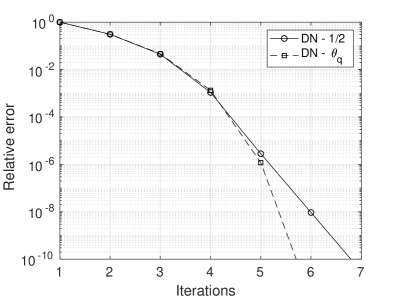
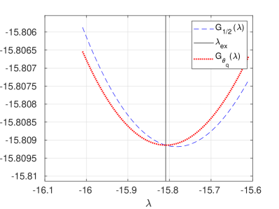
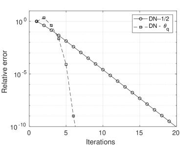
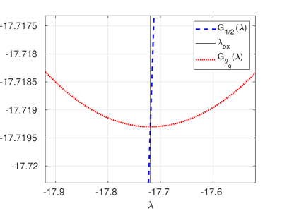
Figure 2: In the left panels, we show the convergence curves, and in the right panels we plot $G_{\theta}(\lambda)$. The top-row refers to a symmetric decomposition, and the bottom-row to an asymmetric one.

we set the interface $\Gamma$ to $x=1/2$. In the left panel, we plot the convergence curves for $\theta=1/2$ and for $\theta_{\text{q}}:=\frac{1}{1+\delta}$. In this setting, $\delta=1.006$ and $\theta_{\text{q}}=0.498$, so due to the symmetry of the decomposition, $\theta_{\text{q}}$ is still very close to $1/2$. In the right panel, we plot $G_{\theta}(\lambda)$ and see that as $\theta$ changes, the minimum of $G_{\theta}(\lambda)$ moves, such that it is attained at $\lambda=\lambda_{\text{ex}}$ for $\theta=\theta_{\text{q}}$.

Next, in the bottom row of Fig 2, we consider the same equation and boundary conditions, but $\Gamma$ is now at $x=0.3$. The decomposition is asymmetric, with $\delta=0.43$ and $\theta_{\text{q}}=0.699$. The left panel shows clearly that for $\theta=1/2$ the convergence is linear, while for $\theta=\theta_{\text{q}}$, the DN method converges quadratically. In the right panel, we observe that $G_{1/2}(\lambda)$ does not have a local extremum at $\lambda=\lambda_{\text{ex}}$, while $G_{\theta_{q}}(\lambda)$ does. Theorem 1 does not easily generalize to higher dimensions, since $\text{DtN}^{\prime}_{j}$ are then matrices, and the relaxation parameter would have to be an operator. Numerically we observed for symmetric decompositions fast convergence for $\theta=0.5$, while for asymmetric decompositions, $\theta$ needs to be tuned for good performance.

3 Mesh independent convergence

One of the attractive features of the DN method for linear problems is that it achieves mesh independent convergence. Does this also hold for the nonlinear DN method (2)? We first define the nonlinear DN method for multiple subdomains. Motivated by the definition of the DN method for the linear case in kumbhar_p_mini_17_scalabilty_CCGT , we divide the domain $\Omega:=(0,L)\times(0,L)$ into $N$ nonoverlapping subdomains $\Omega_{j}=(\Gamma_{j-1},\Gamma_{j})\times(0,L)$, with $\Gamma_{0}=0$ and $\Gamma_{N}=L$. The nonlinear DN method for multiple subdomains is then defined for the interior subdomains by

$$\begin{array}[]{rcll}\mathcal{L}(u^{n}_{j})&=&f_{j}&\text{in $\Omega_{j}$},\\ \mathcal{N}_{j}u^{n}_{j}(\Gamma_{j-1},\cdot)&=&-\mathcal{N}_{j-1}u^{n}_{j-1}(\Gamma_{j-1},\cdot)&\text{on$\quad\Gamma_{j-1}$},\\ u^{n}_{j}(\Gamma_{j})&=&(1-\theta)u^{n-1}_{j}(\Gamma_{j},\cdot)+\theta u^{n-1}_{j+1}(\Gamma_{j},\cdot)&\text{on $\Gamma_{j}$},\end{array}$$

where $\theta\in(0,1)$, and for the left and right most subdomains by

$$\begin{array}[]{rclrcl}\mathcal{L}(u_{1}^{n})&=&f_{1},\quad\text{in}\quad\Omega_{1},&\mathcal{L}(u_{N}^{n})&=&f_{N},\quad\text{in}\quad\Omega_{N},\\ u^{n}_{1}(\Gamma,\cdot)&=&g(0),&\mathcal{N}_{N}u^{n}_{N}(\Gamma_{N-1},\cdot)&=&-\mathcal{N}_{N-1}u^{n}_{N-1}(\Gamma_{N-1},\cdot),\\ u^{n}_{1}(\Gamma_{1},\cdot)&=&(\!1\!-\!\theta\!)u^{n-1}_{1}(\Gamma_{1},\cdot)\!+\!\theta u^{n-1}_{2}(\Gamma_{1},\cdot),&u^{n}_{N}(L,\cdot)&=&g(L).\end{array}$$

We perform two experiments, one in 1D and one in 2D. For the 1D case, we consider the nonlinear diffusion equation $-\partial_{x}\left((1+u^{2})\partial_{x}u\right)=0$, with $u(0)=0$ and $u(1)=20$. We divide the domain $\Omega=(0,1)$ into ten equal subdomains. We then plot the relative error of the nonlinear DN for four different mesh sizes $h$=1e-2, $h$=2e-3, $h$=1e-3, and $h$=1e-4. The left plot in Fig. 3

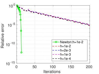
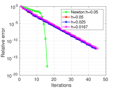
Figure 3: Convergence behavior of nonlinear DN for different mesh sizes in 1D (left) and 2D (right).

shows that the convergence rate of the nonlinear DN is independent of mesh size, while it is quadratic for Newton’s Method. We repeat a similar experiment in 2D, but now the domain $\Omega=(0,1)\times(0,1)$ is divided into four equal subdomains. Even in 2D, we observe the mesh independent convergence of the nonlinear DN method, see the right plot of Fig. 3.

4 Dirichlet-Neumann Preconditioned Exact Newton (DNPEN)

In Section 2, we observed that under some special conditions on the exact solution of the nonlinear problem and $\theta$, the nonlinear DN method (2) can be nilpotent. Moreover, the nonlinear DN method can also converge quadratically. But to achieve this, we need to tune the parameter $\theta$ according to some a priori knowledge of the exact solution of the nonlinear problem. Thus in general, the nonlinear DN method converges linearly (as shown in Fig 3).

Iterative methods can be used as preconditioners to achieve faster convergence, see kumbhar_p_mini_17_bookCG for the linear case, and kumbhar_p_mini_17_gander2017origins for a historical introduction including also the nonlinear case. It was proposed in kumbhar_p_mini_17_dolean2016nonlinear ; kumbhar_p_mini_17_SUBRAS to use the nonlinear Restricted Additive Schwarz (RAS) and nonlinear Substructured RAS (SRAS) methods as preconditioner for Newton’s method. We use the same idea here and apply Newton’s method to the fixed point equation of the nonlinear DN method (3), which represents a systematic way of constructing non-linear preconditioners kumbhar_p_mini_17_gander2017origins . The fixed point version of (3) can be written as

$$\mathcal{F}(\mathbf{\lambda}):=\lambda-G(\lambda)=\theta\lambda-\theta\text{NtD}_{2}\left(-\text{DtN}_{1}\left(\lambda,\psi_{1}\right),\psi_{2}\right).$$ (10)

Applying Newton to (10) we obtain a new method called Dirichlet Neumann Preconditioned Exact Newton (DNPEN) method.

We saw in Section 2 that the DN method can be nilpotent in certain cases. Can DNPEN still be nilpotent? Let $\lambda_{\text{ex}}$ denote the fixed point of the iteration (3). Let us assume that the Dirichlet Neumann method converges in one iteration. This means that $G$ defined in (3) satisfies $\lambda_{\text{ex}}=G(\lambda^{0})$ for any initial guess $\lambda^{0}$. This shows that the map $G$ is constant, and hence $\mathcal{F}^{\prime}(\lambda)$ reduces to the identity matrix. Moreover, one step of Newton’s method applied to (3) can then be written as

$$\lambda^{1}=\lambda^{0}-(\mathcal{F}^{\prime}(\lambda^{0}))^{-1}\mathcal{F}(\lambda^{0})=\lambda^{0}-\mathcal{F}(\lambda^{0})=G(\lambda^{0})=\lambda_{\text{ex}},$$

and hence DNPEN will also be nilpotent in that case. We further have also the following result.

Theorem 4.1

The convergence of DNPEN does not depend on the relaxation parameter $\theta$ in the DN preconditioner.

Proof

The function $\mathcal{F}$ from (10) corresponding to DNPEN can we rewritten as $\mathcal{F}(\lambda)=\theta\mathcal{K}(\lambda,\psi_{1},\psi_{2})$, where $\mathcal{K}(\lambda,\psi_{1},\psi_{2}):=\lambda-\text{NtD}_{2}\left(-\text{DtN}_{1}\left(\lambda,\psi_{1}\right),\psi_{2}\right)$. Thus, Newton’s iteration reads

$$\lambda^{k+1}\!=\!\lambda^{k}-\left(J\mathcal{F}(\lambda^{k})\right)^{-1}\!\!\mathcal{F}(\lambda^{k})\!=\!\lambda^{k}-\left(\theta J\mathcal{K}(\lambda^{k})\right)^{-1}\!\!\theta\mathcal{K}(\lambda^{k})\!=\!\lambda^{k}-\left(J\mathcal{K}(\lambda^{k})\right)^{-1}\!\!\mathcal{K}(\lambda^{k}),$$

which shows that the Newton correction does not depend on the relaxation parameter $\theta$. The iterates of Newton’s method will thus only depend on $\mathcal{K}$, and DNPEN has $\theta$ independent convergence.

The above theorem shows that when using DNPEN, one does not need to search for an optimal choice of $\theta$, in contrast to the nonlinear DN method (2).

We now compare the convergence of DNPEN, the unpreconditioned Newton method, the nonlinear DN method (2) and RASPEN kumbhar_p_mini_17_dolean2016nonlinear . We consider the nonlinear diffusion problem $-\partial_{x}\left(\left(1+u^{2}\right)\partial_{x}u\right)=f$ on $\Omega=(0,1)$ decomposed into two equally sized subdomains, with $u(0)=0$, $u(1)=10$ and $f(x)=\sin(10\pi x)$. For both DN and DNPEN, we choose the optimal relaxation parameter provided in Theorem 2.1. The left plot in Fig. 4

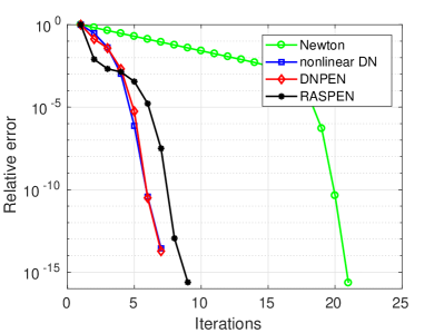
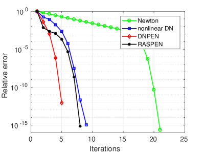
Figure 4: Comparison of DNPEN (with optimal $\theta$) with unpreconditioned Newton, nonlinear DN (with optimal $\theta$) and RASPEN for a symmetric partition (left) and an asymmetric partition (right).

shows that the iterative DN converges quadratically using the optimal parameter and is very similar to DNPEN with no significant gain in the number of iterations. The convergence curves also show that the unpreconditioned Newton method is slower than all preconditioned ones, and DNPEN has a slight advantage over RASPEN.

We repeat the same experiment but now using an asymmetric partition of the domain $\Omega$. The right plot in Fig. 4 shows that for this configuration, DNPEN is the fastest while again unpreconditioned Newton is the slowest among the methods considered. Moreover, DNPEN is significantly faster than the nonlinear DN method.

Finally, we illustrate numerically that the convergence of DNPEN does not depend on $\theta$. We know that in general, the nonlinear DN method converges linearly, and it is not always possible to find an optimal $\theta$ such that it converge quadratically. We again consider the symmetric partition of the domain and use the same boundary conditions and force term as above. However, instead of the optimal $\theta$, we consider two non-optimal $\theta$’s, namely $\theta=0.1$ and $\theta=0.9$. The left plot in Fig. 5

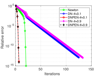
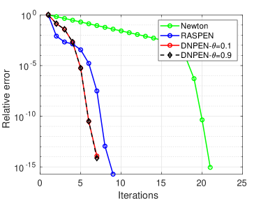
Figure 5: Comparison of DNPEN with the unpreconditioned Newton method and nonlinear DN (left) and with RASPEN (right) for two different non optimal $\theta$’s.

shows the linear convergence of nonlinear DN for both $\theta=0.1$, and $\theta=0.9$, and both are slower than the unpreconditioned Newton method. However, DNPEN converges much faster than Newton’s method and in the same number of iterations for the two different values $\theta=0.1$ and $\theta=0.9$. The right plot in Fig. 5 shows that DNPEN is still faster than RASPEN for both values $\theta$ considered.

5 Conclusion

While iterative DN methods are known to converge linearly, we proved that one can obtain quadratic converge for some one-dimensional nonlinear problems and for a well chosen relaxation parameter $\theta$. Under specific conditions, the nonlinear DN method can also become a direct solver, like in the linear case. We then extended DN to multiple subdomains and numerically showed that its convergence is mesh independent. We finally introduced the nonlinear preconditioner DNPEN, proved that the convergence of DNPEN does not depend on the relaxation parameter $\theta$, and observed numerically that DNPEN is faster than unpreconditioned Newton, nonlinear DN and RASPEN in all our examples.

References

- [1] X-C. Cai and M. Dryja. Domain decomposition methods for monotone nonlinear elliptic problems. Domain Decomposition Methods in Scientific and Engineering, 180:21–27, 1994.
- [2] F. Chaouqui, G. Ciaramella, M. J. Gander, and T. Vanzan. On the scalability of classical one-level domain-decomposition methods. Vietnam J. Math, 46(6):1053–1088, 2018.
- [3] F. Chaouqui, M. J. Gander, P.M. Kumbhar, and T. Vanzan. Linear and Nonlinear Substructured Restricted Additive Schwarz Iterations and Preconditioning. arXiv:2103.16999, 2021.
- [4] G. Ciaramella and M.J Gander. Iterative Methods and Preconditioners for Systems of Linear Equations. Accepted for publication in SIAM, 2022.
- [5] P.G. Ciarlet. Linear and Nonlinear Functional Analysis with Applications. Applied mathematics. SIAM, Philadelphia, PA, 2013.
- [6] V. Dolean, M. J. Gander, W. Kheriji, F. Kwok, and R. Masson. Nonlinear preconditioning: How to use a nonlinear Schwarz method to precondition Newton’s method. SIAM Journal on Scientific Computing, 38(6):A3357–A3380, 2016.
- [7] L.C. Evans. Partial Differential Equations. Graduate studies in mathematics. American Mathematical Society, 2010.
- [8] Martin J. Gander. On the origins of linear and non-linear preconditioning. In Domain Decomposition Methods in Science and Engineering XXIII, pages 153–161. Springer, 2017.
- [9] Alfio Quarteroni and Alberto Valli. Domain decomposition methods for partial differential equations. Oxford University Press, 1999.