The Southern H ii Region Discovery Survey II: The Full Catalog

Abstract

The Southern H ii Region Discovery Survey (SHRDS) is a 900 hour Australia Telescope Compact Array 4–10$\,{\rm GHz}$ radio continuum and radio recombination line (RRL) survey of Galactic H ii regions and infrared-identified H ii region candidates in the southern sky. For this data release, we reprocess all previously published SHRDS data and include an additional ${\sim}450$ hours of observations. The search for new H ii regions is now complete over the range $259^{\circ}<\ell<346^{\circ},|{\it b}|<4^{\circ}$ for H ii region candidates with predicted $6\,{\rm GHz}$ continuum peak brightnesses $\,\gtrsim\,30\,\text{mJy beam}^{-1}$. We detect radio continuum emission toward 730 targets altogether including previously known nebulae and H ii region candidates. By averaging ${\sim}18$ RRL transitions, we detect RRL emission toward 206 previously known H ii regions and 436 H ii region candidates. Including the northern sky surveys, over the last decade the H ii Region Discovery Surveys have more than doubled the number of known Galactic H ii regions. The census of H ii regions in the WISE Catalog of Galactic H ii Regions is now complete for nebulae with 9$\,{\rm GHz}$ continuum flux densities $\,\gtrsim\,250\,\text{mJy}$. We compare the RRL properties of the newly discovered SHRDS nebulae with those of all previously known H ii regions. The median RRL full-width at half-maximum line width of the entire WISE Catalog H ii region population is $23.9\,{\rm km\,s^{-1}}$ and is consistent between Galactic quadrants. The observed Galactic longitude-velocity asymmetry in the population of H ii regions probably reflects underlying spiral structure in the Milky Way.

1 Introduction

H ii regions are the zones of ionized gas surrounding young, massive stars. These nebulae are the archetypical tracer of spiral arms and gas-phase metallicity structure in galaxies. Their physical properties (e.g., electron density, electron temperature, metallicity) inform our understanding of high-mass star formation (e.g., Churchwell, 2002), the interstellar medium (ISM; e.g., Luisi et al., 2016), and Galactic chemical evolution (e.g., Wenger et al., 2019a). A complete census of Galactic H ii regions will place constraints on models of Milky Way formation and evolution, but a lack of sensitive surveys in the southern sky has left this census incomplete.

Dedicated searches for Galactic H ii regions began nearly seven decades ago with the photographic plate surveys of Sharpless (1953) and Sharpless (1959) in the northern hemisphere and Gum (1955) and Rodgers et al. (1960) in the southern hemisphere. The prediction (Kardashev, 1959) and discovery (Hoglund & Mezger, 1965a, b) of radio recombination lines (RRLs) provided a new, extinction-free spectroscopic tracer of Galactic H ii regions. Over the next several decades, RRL surveys discovered hundreds of new nebulae, the majority of which are optically obscured (e.g., Reifenstein et al., 1970; Wilson et al., 1970; Downes et al., 1980; Caswell & Haynes, 1987; Lockman, 1989; Lockman et al., 1996). See Wenger et al. (2019b, the Bright Catalog; hereafter, Paper I) for a brief review of the history of H ii region RRL surveys.

The Wide-field Infrared Survey Explorer (WISE) Catalog of Galactic H ii Regions (Anderson et al., 2014, hereafter, the WISE Catalog) requires the detection of recombination line emission, such as H$\alpha$ or RRL emission, to classify a nebula as a known H ii region. This is a conservative definition of an H ii region. Other studies have less restrictive criteria for H ii region classification. For example, the presence of ionized gas in nebulae has been inferred from radio continuum spectral energy distributions (e.g., Becker et al., 1994) and/or infrared colors (e.g., Wood & Churchwell, 1989; White et al., 1991), although these techniques sometimes suffer from contamination by other Galactic objects such as planetary nebulae or high-mass evolved stars (e.g., Leto et al., 2009). Recombination line emission is unambiguous evidence for the presence of thermally-emitting plasma.

The Southern H ii Region Discovery Survey (SHRDS) is the final component of the H ii Region Discovery Survey (HRDS; Bania et al., 2010). The original Green Bank Telescope (GBT) HRDS discovered 602 hydrogen RRLs toward 448 H ii region candidates in the zone $67^{\circ}\leq\ell\leq 343^{\circ};|{\it b}|\leq 1^{\circ}$. These candidates were selected based on their spatially coincident radio continuum and 24 $\mu$m emission (Anderson et al., 2011). Subsequent HRDS papers derived kinematic distances (Anderson et al., 2012) and characterized the helium and carbon RRLs (Wenger et al., 2013) for a subset of these nebulae. Additional surveys made with the Arecibo Telescope (Bania et al., 2012) and the GBT (Anderson et al., 2015, 2018) extended the HRDS. Altogether, the HRDS discovered 887 new Galactic H ii regions in the northern sky.

The SHRDS extends the HRDS to the southern sky. We use the Australia Telescope Compact Array (ATCA) to search for 4–10$\,{\rm GHz}$ radio continuum and RRL emission toward infrared-identified H ii region candidates in the 3rd and 4th Galactic quadrants. In the pilot survey (Brown et al., 2017) and first data release (Paper I), we found RRL emission toward 295 new Galactic H ii regions, nearly doubling the number of known nebulae in the survey zone.

The Full Catalog presented in this paper is the final SHRDS data release. We add an additional ${\sim}450$ hours of observations not included in Paper I and also reanalyze all the previous SHRDS data. By reprocessing all of the data in a uniform and consistent manner, we minimize any systematic discrepancies between data releases. This data release supersedes the Pilot survey (Brown et al., 2017) and Paper I. Although the data reduction and analysis steps are similar, we make several changes to improve the data quality and maximize our detection rate. Furthermore, we include here intermediate data products, such as the properties of individual RRL transitions, which can be used to study specific nebulae in detail.

2 Target Sample

We select the SHRDS H ii region candidate targets from the WISE Catalog. In Paper I, we targeted nebulae with predicted 6$\,{\rm GHz}$ continuum brightnesses $\,\gtrsim\,60\,\text{mJy beam}^{-1}$ based on extrapolated Sydney University Molonglo Sky Survey (SUMSS) 843$\,{\rm MHz}$ flux densities and an assumed optically thin spectral index of $\alpha=-0.1$. For the Full Catalog, we add those WISE Catalog objects with predicted brightnesses between $30$ and $60\,\text{mJy beam}^{-1}$ and infrared diameters smaller than $5{{}^{\prime}}$. The optically thin assumption is likely invalid at frequencies $\lesssim 1\,{\rm GHz}$, and indeed we find a scatter of ${\sim}100\%$ between the extrapolated and measured 6$\,{\rm GHz}$ flux densities of nebulae in the Bright Catalog (see Paper I, ). Objects in the WISE Catalog that do not meet our brightness criterion may be nebulae ionized by lower-mass stars (B-stars), very distant, or optically thick.

As both a test of our experiment and to improve the accuracy and reliability of the previous single dish RRL detections, we also observe 175 previously known H ii regions. These nebulae have previous RRL detections made with the Parkes telescope (Caswell & Haynes, 1987), the GBT as part of the HRDS, or the Jansky Very Large Array (VLA; Wenger et al., 2019a). The Caswell & Haynes (1987) RRL survey has an angular resolution of ${\sim}4.4{{}^{\prime}}$, which is insufficient to disentangle the RRL emission from multiple H ii regions in confusing fields. The GBT HRDS and VLA data overlap with the higher frequency end of the SHRDS (${\sim}$8–10$\,{\rm GHz}$) and have comparable (${\sim}90{{{}^{\prime\prime}}}$ for GBT HRDS) or finer (${\sim}10{{{}^{\prime\prime}}}$ for VLA) angular resolution. We test our experiment by comparing the RRL properties (e.g., line width) measured by the SHRDS with those previous detections.

The target list for the full SHRDS includes 435 H ii region candidates and 175 previously known H ii regions. The ATCA has a large field of view (primary beam half-power beam width, HPBW, ${\sim}4{{}^{\prime}}$ at $8\,{\rm GHz}$) so multiple WISE catalog sources can appear within a single pointing. Table 3 gives information about the H ii regions and H ii region candidates in each SHRDS field: the field name, the field center position, and every WISE catalog source within that field. For each source, we list: the WISE catalog source name, the source type (“K” for previously known H ii region; “C” for H ii region candidate; “Q” for radio-quiet H ii region candidate, which lacks detected radio continuum emission in extant surveys; and “G” for a candidate associated with a known group of H ii regions), the WISE infrared position, the WISE infrared radius, and the reference to the previous non-SHRDS RRL detection, if any.

3 Observations, Data Reduction & Analysis

The observing strategy and data processing procedure for the Full Catalog are similar to that of Paper I. We used the ATCA C/X-band receiver and Compact Array Broadband Backend (CABB) to simultaneously observe 4–8$\,{\rm GHz}$ radio continuum emission and 20 hydrogen RRL transitions in two orthogonal linear polarizations (note that Paper I incorrectly states that circular polarizations were observed). Our observations took place between June 2015 and January 2019 with a total of 900 hours of telescope time split equally between the H75 and H168 antenna configurations. We observed each field for a total of ${\sim}30$ to ${\sim}90$ minutes in ${\sim}5$ to ${\sim}10$ minute snapshots spread over ${\sim}9$ hours in hour angle. See Tables 2 and 3 for a summary of the observations and spectral window configuration, respectively.

The ATCA with CABB is an excellent tool for discovering RRLs toward Galactic H ii regions. In our hybrid H75/H168 data, the synthesized HPBW (${\sim}90{{{}^{\prime\prime}}}$ at ${\sim}8\,{\rm GHz}$) is well-matched to the typical classical H ii region diameter (90^′′is equivalent to a 10 pc diameter at 20 kpc distance). The compact antenna configurations yield a good surface brightness sensitivity for resolved nebulae, and the large collecting area yields a good point-source sensitivity for unresolved nebulae. The large bandwidth and flexible backend allow for the simultaneous observation of 20 RRL transitions, which we average to improve the spectral sensitivity. See Paper I for representative SHRDS images and RRL spectra.

We use the Wenger Interferometry Software Package (WISP; Wenger, 2018) to calibrate, reduce, and analyze the SHRDS data. See Paper I for details regarding the calibration of the SHRDS data. WISP is a wrapper for the Common Astronomy Software Applications package (CASA; McMullin et al., 2007). WISP uses automatic flagging and CLEAN region identification to reduce the burden of interferometric data processing, which can be extremely time intensive. WISP is well-tested on both ATCA and VLA radio continuum and spectral line data (Wenger et al., 2019a, b).

For each observed field the WISP imaging pipeline produces the following data products: a 4$\,{\rm GHz}$ bandwidth multi-scale, multi-frequency synthesis (MS-MFS) continuum image, sixteen 256$\,{\rm MHz}$ bandwidth MS-MFS continuum images covering the full 4$\,{\rm GHz}$ bandwidth, a MS-MFS continuum image of each 64$\,{\rm MHz}$ bandwidth spectral line window, and a multi-scale data cube of each spectral line window. The first and last of the 256$\,{\rm MHz}$ bandwidth continuum images are compromised by radio-frequency interference (RFI) and band-edge effects and are typically unusable.

Unlike Paper I, we image each spectral line data cube at its native spectral resolution. Since the RRLs span almost a factor of two in frequency, the velocity resolution of our spectral line windows varies by nearly a factor of two as well. The spectra must be sampled or re-gridded on a common velocity axis in order to average the individual RRL spectra and create the $\langle\text{Hn}\alpha\rangle$ average spectrum. We improve the sensitivity of our average spectra by smoothing the higher resolution spectra to match the lowest resolution observed. Paper I uses linear interpolation (without smoothing) to re-grid the spectra. Here we use sinc interpolation to both smooth and re-grid the RRL spectra to a common velocity axis (see Appendix A). This method results in a ${\sim}20\%$ sensitivity improvement in the $\langle\text{Hn}\alpha\rangle$ average spectra compared to the Paper I analysis.

Table 1: Full Catalog Fields and Targets

Field	RA	Dec.	Target	Catalog	RA	Dec.	$R_{\rm IR}$	Author
	J2000	J2000			J2000	J2000	(arcsec)
	(hh:mm:ss)	(dd:mm:ss)			(hh:mm:ss)	(dd:mm:ss)
ch1	07:30:05.8	$-18$:32:27.2	G233.676$-$00.186	Q	07:29:56.6	$-18$:27:50.1	$59.11$
			G233.753$-$00.193	K	07:30:04.6	$-18$:32:03.9	$311.06$	B11
			G233.830$-$00.180	G	07:30:16.9	$-18$:35:44.5	$114.85$
ch4	08:20:56.3	$-36$:12:32.0	G254.682+00.220	K	08:20:55.5	$-36$:13:09.9	$385.32$	CH87
shrds027	08:23:21.5	$-40$:39:59.7	G258.608$-$01.925	Q	08:23:21.7	$-40$:39:57.7	$136.61$
shrds029	08:26:13.4	$-40$:46:45.4	G259.013$-$01.546	Q	08:26:13.5	$-40$:46:45.0	$68.08$
			G259.057$-$01.544	C	08:26:22.1	$-40$:48:49.5	$103.98$
			G259.086$-$01.612	C	08:26:09.9	$-40$:52:36.2	$103.98$
shrds030	08:26:18.8	$-40$:48:36.5	G259.013$-$01.546	Q	08:26:13.5	$-40$:46:45.0	$68.08$
			G259.057$-$01.544	C	08:26:22.1	$-40$:48:49.5	$103.98$
			G259.086$-$01.612	C	08:26:09.9	$-40$:52:36.2	$103.98$

Note. — This table is available in its entirety in a machine-readable form in the online journal. A portion is shown here for guidance regarding its form and content.

References. — (GBT HRDS) Anderson et al. (2011, 2015, 2018); (B11) Balser et al. (2011); (CH87) Caswell & Haynes (1987); (D80) Downes et al. (1980); (L89) Lockman (1989); (Q06) Quireza et al. (2006); (S04) Sewilo et al. (2004); (W70) Wilson et al. (1970)

Table 2: Observation Summary

Observing Dates	2015$-$07$-$24 to 2019$-$01$-$25
Observing Time	900 hr
Primary Calibrators	0823$-$500, 1934$-$638
Secondary Calibrators	0906$-$47, 1036$-$52, j1322$-$6532, 1613$-$586
	1714$-$397, 1714$-$336, 1829-207

In the Full Catalog, we use the polarization data to generate full-Stokes (IQUV) MS-MFS images of the 4$\,{\rm GHz}$ bandwidth continuum image and each 256$\,{\rm MHz}$ bandwidth continuum image. To calibrate the polarization data, we assume that the primary calibrator 1934$-$638 is unpolarized and any observed polarized emission is due to instrumental leakage. We use the 1934$-$638 data to derive the instrumental polarization leakage corrections. After applying these leakage corrections to the secondary calibrators, we derive the Stokes polarization fractions ($Q/I$, $U/I$, and $V/I$) for each secondary calibrator, update the secondary calibrator flux model with these polarization fractions, and recompute the complex gain calibration tables. Finally, we apply all of the calibration tables, including the polarization leakage calibration tables, to the science targets. This polarization calibration prescription is included in the latest WISP release.

Table 3: Spectral Window Configuration

Window	Center Freq.	Bandwidth	Channels	Channel Width	RRL	Rest Freq.
	(MHz)	(MHz)		(kHz)		(MHz)
0	4545	256	4	64000	…	…
1	4801	256	4	64000	…	…
2	5057	256	4	64000	…	…
3	5313	256	4	64000	…	…
4	5569	256	4	64000	…	…
5	5825	256	4	64000	…	…
6	6081	256	4	64000	…	…
7	6337	256	4	64000	…	…
8	7580	256	4	64000	…	…
9	7836	256	4	64000	…	…
10	8092	256	4	64000	…	…
11	8348	256	4	64000	…	…
12	8604	256	4	64000	…	…
13	8860	256	4	64000	…	…
14	9116	256	4	64000	…	…
15	9372	256	4	64000	…	…
16	4609	64	2049	31.25	H112$\alpha$	4618.790
17	4737	64	2049	32.25	H111$\alpha$	4744.184
18	4865	64	2049	31.25	H110$\alpha$	4874.158
19	4993	64	2049	31.25	H109$\alpha$	5008.924
20	5153	64	2049	31.25	H108$\alpha$	5148.704
21	5281	64	2049	31.25	H107$\alpha$	5293.733
22	5441	64	2049	31.25	H106$\alpha$	5444.262
23	5601	64	2049	31.25	H105$\alpha$	5600.551
24	5761	64	2049	31.25	H104$\alpha$	5762.881
25	5921	64	2049	31.25	H103$\alpha$	5931.546
26	6113	64	2049	31.25	H102$\alpha$	6106.857
27	6305	64	2049	31.25	H101$\alpha$	6289.145
28	6465	64	2049	31.25	H100$\alpha$	6478.761
29	7548	64	2049	31.25	H95$\alpha$	7550.616
30	7804	64	2049	31.25	H94$\alpha$	7792.872
31	8060	64	2049	31.25	H93$\alpha$	8045.604
32	8316	64	2049	31.25	H92$\alpha$	8309.384
33	8572	64	2049	31.25	H91$\alpha$	8584.823
34	9180	64	2049	31.25	H89$\alpha$	9173.323
35	8500	64	2049	31.25	H88$\alpha$	9487.823

We do not perform any uv-tapering when imaging SHRDS Full Catalog fields. Tapering can improve surface brightness sensitivity at the expense of angular resolution. In Paper I, we uv-tapered all data to a ${\sim}100{{{}^{\prime\prime}}}$ angular resolution and then smoothed these images to a common angular resolution. By the convolution theorem, smoothing by convolving the images with a Gaussian kernel is equivalent to uv-tapering by weighting the uv-data with a Gaussian function (Oppenheim et al., 1975). Therefore, we save processing time and disk space by skipping the uv-tapering step and instead smooth the non-tapered data to a common angular resolution. In principle, we might lose sensitivity to diffuse emission that is not bright enough to be CLEANed in the non-tapered images. Our surface brightness sensitivity, however, is excellent due to the compact antenna configuration and comprehensive uv-coverage, and tests with uv-tapering reveal no noticeable improvement in sensitivity compared to the smoothed images.

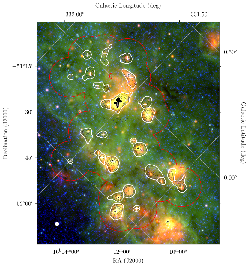
Figure 1: The largest SHRDS radio continuum mosaic, mos040, overlaid on 3.4$\mu$m (blue), 12$\mu$m (green), and 22$\mu$m (red) data from the WISE All-Sky Survey (Wright et al., 2010). Black regions in the image are saturated in at least one WISE band. The black contours are the mosaicked 4$\,{\rm GHz}$ bandwidth radio continuum data at 5, 10, 20, 50, 100, and 200 times the image rms. The red contour represents the 10% primary beam response and the extent of the SHRDS data. Each white cross is the location of the brightest pixel associated with a WISE Catalog source and each white contour is the watershed region for that source. The filled white circle in the lower left is the smoothed resolution of the radio continuum data.

We extract spectra and measure the total flux densities of the SHRDS nebulae using the watershed segmentation technique of Wenger et al. (2019a). Given an image, the watershed segmentation algorithm identifies all pixels with emission associated with an emission peak (the “watershed region;” see Bertrand, 2005). If two or more peaks are close together, then the algorithm will split the emission into that many non-overlapping watershed regions. As in Paper I, we first identify continuum detections as any emission peaks that are (1) brighter than 5 times the rms noise in the 4$\,{\rm GHz}$ bandwidth MS-MFS image and (2) within the circle defined by the WISE Catalog infrared position and radius. To estimate the rms noise across the image, we divide the standard deviation of the residual image by the primary beam response. Hereafter, the location of the emission peak in the 4$\,{\rm GHz}$ bandwidth MS-MFS image is called the source position. For each continuum detection we measure the peak continuum brightness at the source position in every MS-MFS image. We extract a spectrum from each data cube at this position as well. The source positions are the starting locations for the watershed segmentation algorithm. We clip each MS-MFS image by masking all pixels fainter than 5 times the rms noise and then apply the watershed algorithm to these clipped images. Following the procedure in Wenger et al. (2019a), we measure total continuum flux densities in each MS-MFS image and extract spectra from every data cube. The total flux density is the sum of the brightness in each pixel within the watershed region. The watershed region spectrum is a weighted average of the spectra extracted from each pixel within the region (see Wenger et al., 2019a).

The SHRDS continuum and RRL flux densities are systematically underestimated. By the nature of an interferometer, we miss flux due to the central “hole” in our uv-coverage. The importance of this effect depends on the uv-coverage of the data and the source brightness distribution. For a Gaussian source brightness distribution, we use equation A6 from Wilner & Welch (1994) to estimate that the SHRDS flux densities are reduced by ${\sim}5\%$. Furthermore, because we use the clipped MS-MFS images to generate the watershed regions, the measured total flux densities are further underestimated. For a Gaussian source brightness distribution, the total flux density is reduced by ${\sim}20\%$ if the peak brightness is ${\sim}10$ times the rms noise and by ${\sim}10\%$ if the peak brightness is ${\sim}20$ times the rms noise. The SHRDS total flux densities may be unreliable if the source has a complicated emission structure. These effects are eliminated in the RRL-to-continuum brightness ratio, however, if both the RRL and continuum flux densities are measured using the same watershed region in the same data cube.

Many individual SHRDS fields overlap due to the large field of view of the ATCA. We improve the sensitivity in the overlapped regions by creating linear mosaics following Cornwell et al. (1993):

$$I^{m}(\theta)=\frac{\sum_{p}A^{2}_{p}(\theta)I_{p}(\theta)}{\sum_{p}A^{2}_{p}(\theta)},$$ (1)

where $I^{m}(\theta)$ is the mosaic datum at sky position $\theta$, $I_{p}(\theta)$ is the non-primary beam corrected datum at $\theta$ in pointing $p$, $A_{p}(\theta)$ is the primary beam weight at $\theta$ in $p$, and the sum is over all overlapping pointings. Thus, each position of the mosaic is the average of each individual image weighted by the square of the primary beam.

We create 99 mosaics by combining the images of 329 individual fields. Table 4 lists the fields that are used to create each mosaic. Using equation 1, we smooth each continuum image and RRL data cube to the worst resolution of the ensemble. We process and analyze each mosaic in the same manner as an individual field. Our largest mosaic, mos040, is the combination of 30 fields centered near $(\ell,{\it b})=(331.5^{\circ},-0.15^{\circ})$. The 4$\,{\rm GHz}$ bandwidth MS-MFS continuum mosaic is shown in Figure 1. The white contours show the watershed regions of the 27 nebulae identified in this mosaic.

4 SHRDS: The Full Catalog

The SHRDS Full Catalog is a compilation of the radio continuum and RRL properties of every H ii region detected in the survey. We observe 609 fields containing 1398 WISE catalog sources. The fields contain 289 previously known H ii regions, 554 H ii region candidates, 385 radio-quiet candidates, and 170 candidates that are associated with an H ii region group (see Table 3). We detect radio continuum emission toward 212 previously known nebulae and 518 H ii region candidates, including 40 radio-quiet and 89 group candidates. Of those, we detect $\langle\text{Hn}\alpha\rangle$ RRL emission toward 204 previously known H ii regions and 428 H ii region candidates, including 14 radio-quiet and 82 group candidates. We do not detect some previously known H ii regions because (1) the nebula is larger than the ATCA maximum recoverable scale (${\sim}200{{{}^{\prime\prime}}}$ at 8$\,{\rm GHz}$) and/or (2) the nebula is near the edge of the primary beam and/or (3) the nebula is confused with a nearby H ii region and thus missed by our source identification method.

Table 4: Mosaic Fields

Mosaic	Fields
mos000	fa489, ch309
mos001	fa054, gs108, ch307
mos002	ch282, ch283
mos003	g351.311+, overlap1
mos004	ch253, ch254
mos005	ch246, caswell25
mos006	ch244, caswell24
mos007	shrds1240, shrds1241
mos008	shrds1238, shrds1239
mos009	ch239, caswell23
mos010	shrds930, shrds931, shrds932
mos011	ch234, shrds1237
mos012	shrds925, g339.717-01.102, shrds923
mos013	ch230, shrds928, shrds922, shrds920, shrds917
	shrds918, shrds921
mos014	shrds913, shrds909, shrds908, shrds1228
mos015	shrds1223, shrds1225, shrds905, shrds906
mos016	shrds896, caswell22, ch221, shrds898, shrds899
	shrds900, shrds901
mos017	shrds878, shrds875, ch214, shrds884, shrds883
	shrds880, shrds885, shrds881, shrds886, shrds888
	shrds1218, shrds890, shrds892, shrds893, shrds1219
	shrds891, shrds1233
mos018	shrds869, shrds870
mos019	shrds866, shrds867, shrds868
mos020	shrds1205, shrds1209, shrds1212, shrds862, shrds864
mos021	shrds854, shrds857, shrds1204
mos022	shrds855, ch209, caswell21
mos023	shrds835, shrds836
mos024	shrds833, shrds834
mos025	caswell20, ch201
mos026	shrds806, shrds807, shrds810, shrds811
mos028	shrds800, shrds801, shrds799, ch196, caswell19
	shrds1200
mos029	shrds801, shrds800, shrds799, shrds802
mos030	shrds785, shrds789, shrds793, ch194
mos031	shrds792, shrds786, shrds788, shrds792, shrds794
mos032	shrds784, ch191
mos033	shrds777, ch190
mos034	shrds773, shrds775
mos035	shrds771, shrds1181
mos036	shrds759, shrds764
mos037	shrds756, shrds763, shrds766
mos038	shrds753, ch186
mos040	shrds709, shrds711, shrds714, shrds716, shrds720
	shrds710, shrds721, shrds717, ch179, ch180
	shrds725, ch181, shrds731, shrds734, shrds732
	shrds735, ch182, shrds729, ch185, shrds733
	shrds736, shrds738, shrds737, shrds736, shrds741
	shrds743, shrds744, shrds746, shrds743, shrds745
mos041	shrds731, shrds735
mos042	shrds723, shrds719
mos043	shrds1171, shrds1172, ch177
mos044	shrds1174, shrds1175g
mos045	shrds677, shrds679, shrds686
mos046	ch171, shrds669
mos047	shrds651, shrds652, shrds659
mos048	ch168, shrds656, shrds657
mos049	shrds634, shrds635, shrds640, shrds639, shrds643
	shrds648, shrds647, shrds644
mos050	shrds1167, ch162, caswell18, shrds1168
mos051	shrds1164, shrds1163, ch156
mos052	ch154, caswell17
mos053	caswell16, ch149
mos054	shrds589, shrds590
mos055	caswell15, ch145, shrds1151
mos056	caswell14, ch144
mos057	shrds1144g, shrds559, shrds1146, shrds1147
mos058	shrds1133g, shrds1134g, ch138, shrds552, ch139
	shrds1139, shrds1140
mos059	ch136, shrds1137
mos060	shrds535, shrds536, ch131
mos061	caswell13, ch129
mos062	shrds501, ch122
mos063	shrds458, shrds462, shrds463
mos064	ch114, ch113, shrds440, shrds435, shrds439
	shrds437
mos065	shrds1103, shrds432
mos066	caswell12, ch110, shrds428
mos067	shrds418, shrds413, shrds1096, shrds1095g, shrds411
	shrds409
mos068	shrds386, shrds385, shrds387
mos069	caswell11, ch96
mos070	shrds377, g308.033-01
mos071	caswell10, shrds365, shrds364, ch94
mos072	shrds308, shrds309
mos073	shrds296, shrds297
mos074	shrds294, shrds295
mos075	ch76, caswell9
mos076	ch73, caswell7, ch74, caswell8
mos077	shrds271, shrds273
mos078	shrds1046, ch71, caswell6
mos079	shrds253, shrds256, shrds261, shrds258, g298.473+
mos080	shrds249, ch66, caswell5
mos081	shrds1041, ch67
mos082	shrds246, ch65
mos083	shrds215, g293.936-, shrds219, g293.994-
mos084	shrds207, ch57
mos085	ch55, caswell4
mos086	ch52, caswell3, shrds1034
mos087	shrds1031g, shrds1032
mos088	shrds1028, shrds191, g290.012-
mos089	ch35, ch36
mos090	shrds1017, shrds1018g
mos091	ch33, shrds143
mos092	ch32, caswell2
mos093	ch19, shrds1007
mos094	shrds1005, ch17, caswell1
mos095	shrds088, shrds089, ch13
mos096	shrds085, ch11, shrds087
mos097	shrds056, shrds057
mos098	shrds055, shrds054
mos099	shrds034, shrds036, shrds037, shrds042
mos100	shrds029, shrds030

As in Paper I, we attempt to reprocess the SHRDS pilot survey data (Brown et al., 2017) with mixed success. Due to the limited uv-coverage of the pilot observations, we are unable to create images for ten pilot fields. Brown et al. (2017) extracted spectra directly from the visibility data. They detected RRL emission toward ten sources in these unimaged fields: two previously known H ii regions (G213.833+00.618 and G313.790+00.705) and eight H ii region candidates (G230.354$-$00.597, G290.012$-$00.867, G290.323$-$02.984, G290.385$-$01.042, G290.674$-$00.133, G291.596$-$00.239, G295.275$-$00.255, G300.972$+$00.994). The RRL data for these nebulae are included in Brown et al. (2017) and Paper I. These RRL detections increase the number of SHRDS RRL detections toward previously known and H ii region candidates to 206 and 436, respectively.

The Full Catalog data products supersede the previous Bright Catalog in Paper I. Due to the differences in the source selection and data analysis procedures, there are 29 Bright Catalog continuum detections and 22 Bright Catalog $\langle\text{Hn}\alpha\rangle$ RRL detections that are not in the Full Catalog. Each of these detections is in confusing fields and our reprocessing has associated the emission with a different, nearby WISE Catalog object.

4.1 Continuum Catalog

The continuum properties of the SHRDS nebulae are summarized in Table 5 (non-smoothed) and Table 6 (smoothed). For each source, we list the WISE Catalog name, position of the continuum emission peak, field name, and quality factor, QF. Then, for each of the continuum spectral window MS-MFS images and the combined 4$\,{\rm GHz}$ bandwidth MS-MFS image, we list the image synthesized frequency, $\nu$, bandwidth, $\Delta\nu$, synthesized beam area, source peak continuum brightness, $S_{C,P}$, watershed region area, and source total continuum flux density, $S_{C,T}$. The total flux density is measured within the watershed region, and the uncertainty is derived following Equation 1 in Wenger et al. (2019a).

The QF is a qualitative assessment of the reliability of the measured source continuum properties. The highest quality detections, QF A, are unresolved, isolated, and near the center of the field. Intermediate quality detections, QF B, are (1) resolved yet compact with a single emission peak, (2) slightly confused, such that its watershed region borders another source’s watershed region, and/or (3) located off-center in the field. The worst quality detections, QF C, have unreliable continuum properties because they are (1) resolved and the emission is not compact with a single, distinct peak, (2) severely confused with other sources, and/or (3) located near the edge of the field. We recommend using only the QF A and B data in subsequent analyses of these data, but we include the QF C data for completeness.

A WISE Catalog source can appear in Tables 5 and 6 multiple times if it is detected in multiple fields and/or mosaics. Each detection in a non-mosaic field is an independent measurement of the source continuum properties. The detection with the best quality factory should be used for subsequent analyses.

Table 5: Un-smoothed Continuum Detections

Source	RA	Dec.	Field	QF	$\nu$		$\Delta\nu$	Beam		$S_{C,P}$			Region	$S_{C,T}$
	J2000	J2000			(MHz)		(MHz)	Area		(mJy beam-1)			Area	(mJy)
	(hh:mm:ss)	(dd:mm:ss)						(arcmin2)					(arcmin2)
G233.753$-$00.193	07:30:02.2	$-18$:32:43.2	ch1	B	7183.3	4000	0.38	67.82	0.70	12.97	686.40 $\,\pm\,$	4.48
					4897.5	256	1.10	216.76	4.84	14.62	1140.07 $\,\pm\,$	18.67
					5153.5	256	0.94	180.97	4.70	12.82	1028.53 $\,\pm\,$	18.30
					5409.5	256	0.92	171.71	4.03	13.06	985.59 $\,\pm\,$	16.04
					5665.5	256	0.78	142.49	3.28	12.31	907.25 $\,\pm\,$	13.76
					5921.6	256	0.74	129.71	3.71	10.71	829.21 $\,\pm\,$	14.89
					6177.6	256	0.63	107.13	3.53	9.49	745.61 $\,\pm\,$	14.29
					6433.6	256	0.62	100.88	6.08	4.96	489.40 $\,\pm\,$	17.59
					7676.7	256	0.40	65.58	2.66	5.30	429.08 $\,\pm\,$	9.98
					7932.7	256	0.39	61.27	3.46	4.10	363.42 $\,\pm\,$	11.53
					8188.8	256	0.37	58.28	3.01	4.29	366.29 $\,\pm\,$	10.48
					8444.8	256	0.38	57.22	3.35	4.00	347.99 $\,\pm\,$	11.15
					8700.8	256	0.33	48.28	2.52	4.13	336.31 $\,\pm\,$	9.12
					8956.8	256	0.35	47.79	3.04	3.62	306.01 $\,\pm\,$	10.00

Note. — This table is available in its entirety in a machine-readable form in the online journal. A portion is shown here for guidance regarding its form and content.

Table 6: Smoothed Continuum Detections

Source	RA	Dec.	Field	QF	$\nu$		$\Delta\nu$	Beam		$S_{C,P}$			Region	$S_{C,T}$
	J2000	J2000			(MHz)		(MHz)	Area		(mJy beam-1)			Area	(mJy)
	(hh:mm:ss)	(dd:mm:ss)						(arcmin2)					(arcmin2)
G233.753$-$00.193	07:30:02.5	$-18$:32:35.2	ch1	A	7183.3	4000	1.93	220.63	2.42	16.07	664.10 $\,\pm\,$	8.17
					4897.5	256	1.93	323.85	7.21	16.30	1135.67 $\,\pm\,$	22.56
					5153.5	256	1.93	307.24	8.04	14.55	1018.01 $\,\pm\,$	23.73
					5409.5	256	1.93	294.36	6.85	15.01	977.50 $\,\pm\,$	20.75
					5665.5	256	1.93	280.84	6.29	14.46	895.09 $\,\pm\,$	18.78
					5921.6	256	1.93	270.68	7.47	12.82	818.87 $\,\pm\,$	20.92
					6177.6	256	1.93	253.83	8.17	11.54	732.00 $\,\pm\,$	21.65
					6433.6	256	1.93	238.27	12.95	7.08	507.68 $\,\pm\,$	26.23
					7676.7	256	1.93	198.04	8.43	7.56	420.34 $\,\pm\,$	18.12
					7932.7	256	1.93	190.27	11.28	5.82	350.02 $\,\pm\,$	21.08
					8188.8	256	1.93	187.30	9.88	6.13	349.67 $\,\pm\,$	19.09
					8444.8	256	1.93	182.55	11.07	5.60	328.90 $\,\pm\,$	20.41
					8700.8	256	1.93	172.65	9.06	5.93	315.09 $\,\pm\,$	17.31
					8956.8	256	1.93	168.60	10.22	5.23	284.94 $\,\pm\,$	18.27

Note. — This table is available in its entirety in a machine-readable form in the online journal. A portion is shown here for guidance regarding its form and content.

Table 7: Un-smoothed Peak RRL Detections

Source	Field	RRL(s)	$\nu$		Comp.	$S_{L}$				$V_{\rm LSR}$				$\Delta V$	$S_{C}$	SNR
			(MHz)			(mJy beam-1)				(km s-1)				(km s-1)	(mJy beam-1)
G233.753$-$00.193	ch1	H88$-$H112	6236.6	a	7.58	0.64	36.50 $\,\pm\,$	1.10	27.60	2.69	145.03 $\,\pm\,$	1.51	11.7
		H100$-$H112	5414.3	a	7.94	0.82	36.70 $\,\pm\,$	1.30	26.60	3.17	176.06 $\,\pm\,$	1.89	9.6
		H88$-$H95	8788.8	a	5.46	0.68	34.90 $\,\pm\,$	2.20	36.31	5.28	48.95 $\,\pm\,$	1.84	7.9
		H106$-$H112	5010.3	a	8.33	1.05	36.90 $\,\pm\,$	1.90	31.33	4.56	206.36 $\,\pm\,$	2.63	7.8
		H100$-$H105	5914.1	a	7.74	1.34	37.50 $\,\pm\,$	1.80	21.46	4.31	138.60 $\,\pm\,$	2.78	5.7
		H112	4618.8	a	$\cdots$	$\cdots$	$\cdots$ $\,\pm\,$	$\cdots$	$\cdots$	$\cdots$	240.98 $\,\pm\,$	7.32	$\cdots$
		H111	4744.2	a	$\cdots$	$\cdots$	$\cdots$ $\,\pm\,$	$\cdots$	$\cdots$	$\cdots$	223.74 $\,\pm\,$	6.61	$\cdots$
		H110	4874.2	a	$\cdots$	$\cdots$	$\cdots$ $\,\pm\,$	$\cdots$	$\cdots$	$\cdots$	225.37 $\,\pm\,$	6.95	$\cdots$
		H109	5008.9	a	$\cdots$	$\cdots$	$\cdots$ $\,\pm\,$	$\cdots$	$\cdots$	$\cdots$	208.47 $\,\pm\,$	7.34	$\cdots$
		H108	5148.7	a	$\cdots$	$\cdots$	$\cdots$ $\,\pm\,$	$\cdots$	$\cdots$	$\cdots$	192.22 $\,\pm\,$	9.50	$\cdots$
		H107	5293.7	a	$\cdots$	$\cdots$	$\cdots$ $\,\pm\,$	$\cdots$	$\cdots$	$\cdots$	182.74 $\,\pm\,$	6.84	$\cdots$
		H106	5444.3	a	$\cdots$	$\cdots$	$\cdots$ $\,\pm\,$	$\cdots$	$\cdots$	$\cdots$	169.35 $\,\pm\,$	5.77	$\cdots$
		H105	5600.6	a	$\cdots$	$\cdots$	$\cdots$ $\,\pm\,$	$\cdots$	$\cdots$	$\cdots$	160.07 $\,\pm\,$	5.69	$\cdots$
		H104	5762.9	a	$\cdots$	$\cdots$	$\cdots$ $\,\pm\,$	$\cdots$	$\cdots$	$\cdots$	146.62 $\,\pm\,$	5.87	$\cdots$
		H103	5931.5	a	9.74	2.69	39.30 $\,\pm\,$	3.00	21.08	8.97	134.30 $\,\pm\,$	5.14	3.9
		H102	6106.9	a	$\cdots$	$\cdots$	$\cdots$ $\,\pm\,$	$\cdots$	$\cdots$	$\cdots$	127.23 $\,\pm\,$	5.52	$\cdots$
		H100	6478.8	a	$\cdots$	$\cdots$	$\cdots$ $\,\pm\,$	$\cdots$	$\cdots$	$\cdots$	108.69 $\,\pm\,$	5.81	$\cdots$
		H94	7792.9	a	$\cdots$	$\cdots$	$\cdots$ $\,\pm\,$	$\cdots$	$\cdots$	$\cdots$	39.89 $\,\pm\,$	4.76	$\cdots$
		H92	8309.4	a	$\cdots$	$\cdots$	$\cdots$ $\,\pm\,$	$\cdots$	$\cdots$	$\cdots$	57.22 $\,\pm\,$	4.79	$\cdots$
		H91	8584.8	a	$\cdots$	$\cdots$	$\cdots$ $\,\pm\,$	$\cdots$	$\cdots$	$\cdots$	56.35 $\,\pm\,$	3.94	$\cdots$
		H89	9173.3	a	$\cdots$	$\cdots$	$\cdots$ $\,\pm\,$	$\cdots$	$\cdots$	$\cdots$	46.92 $\,\pm\,$	4.00	$\cdots$
		H88	9487.8	a	7.17	1.48	35.40 $\,\pm\,$	3.40	31.75	11.24	42.27 $\,\pm\,$	3.37	5.3

Note. — This table is available in its entirety in a machine-readable form in the online journal. A portion is shown here for guidance regarding its form and content.

Table 8: Smoothed Peak RRL Detections

Source	Field	RRL(s)	$\nu$		Comp.	$S_{L}$				$V_{\rm LSR}$				$\Delta V$	$S_{C}$	SNR
			(MHz)			(mJy beam-1)				(km s-1)				(km s-1)	(mJy beam-1)
G233.753$-$00.193	ch1	H88$-$H112	6326.4	a	16.70	0.82	35.80 $\,\pm\,$	0.60	24.66	1.40	279.29 $\,\pm\,$	1.83	20.1
		H100$-$H112	5440.4	a	16.42	0.99	36.10 $\,\pm\,$	0.70	24.94	1.74	315.59 $\,\pm\,$	2.22	16.3
		H88$-$H95	8852.0	a	17.51	1.47	35.10 $\,\pm\,$	1.00	24.11	2.34	175.60 $\,\pm\,$	3.23	11.8
		H106$-$H112	4992.8	a	16.44	1.30	36.60 $\,\pm\,$	1.10	29.05	2.66	337.54 $\,\pm\,$	3.15	12.5
		H100$-$H105	5916.6	a	16.33	1.55	35.60 $\,\pm\,$	1.00	22.29	2.44	292.31 $\,\pm\,$	3.27	10.4
		H112	4618.8	a	$\cdots$	$\cdots$	$\cdots$ $\,\pm\,$	$\cdots$	$\cdots$	$\cdots$	357.49 $\,\pm\,$	8.27	$\cdots$
		H111	4744.2	a	$\cdots$	$\cdots$	$\cdots$ $\,\pm\,$	$\cdots$	$\cdots$	$\cdots$	341.78 $\,\pm\,$	7.40	$\cdots$
		H110	4874.2	a	21.38	4.45	33.70 $\,\pm\,$	1.70	16.66	4.45	349.38 $\,\pm\,$	7.91	4.9
		H109	5008.9	a	$\cdots$	$\cdots$	$\cdots$ $\,\pm\,$	$\cdots$	$\cdots$	$\cdots$	340.55 $\,\pm\,$	8.20	$\cdots$
		H108	5148.7	a	$\cdots$	$\cdots$	$\cdots$ $\,\pm\,$	$\cdots$	$\cdots$	$\cdots$	335.95 $\,\pm\,$	12.10	$\cdots$
		H107	5293.7	a	19.97	3.47	30.60 $\,\pm\,$	2.10	24.10	5.31	320.83 $\,\pm\,$	7.43	5.8
		H106	5444.3	a	19.87	3.35	35.40 $\,\pm\,$	1.80	22.19	4.40	317.49 $\,\pm\,$	7.03	5.9
		H105	5600.6	a	15.54	3.46	36.50 $\,\pm\,$	2.70	23.62	7.74	306.62 $\,\pm\,$	7.09	4.7
		H104	5762.9	a	14.68	3.15	35.20 $\,\pm\,$	3.20	28.49	10.10	302.97 $\,\pm\,$	6.89	5.0
		H103	5931.5	a	19.62	3.41	38.20 $\,\pm\,$	2.00	23.44	5.29	291.27 $\,\pm\,$	7.17	5.9
		H102	6106.9	a	$\cdots$	$\cdots$	$\cdots$ $\,\pm\,$	$\cdots$	$\cdots$	$\cdots$	283.81 $\,\pm\,$	5.99	$\cdots$
		H100	6478.8	a	$\cdots$	$\cdots$	$\cdots$ $\,\pm\,$	$\cdots$	$\cdots$	$\cdots$	257.65 $\,\pm\,$	7.02	$\cdots$
		H94	7792.9	a	$\cdots$	$\cdots$	$\cdots$ $\,\pm\,$	$\cdots$	$\cdots$	$\cdots$	132.06 $\,\pm\,$	11.06	$\cdots$
		H92	8309.4	a	$\cdots$	$\cdots$	$\cdots$ $\,\pm\,$	$\cdots$	$\cdots$	$\cdots$	197.15 $\,\pm\,$	7.15	$\cdots$
		H91	8584.8	a	18.67	2.60	34.40 $\,\pm\,$	1.80	26.26	4.48	180.10 $\,\pm\,$	5.86	7.2
		H89	9173.3	a	15.90	3.11	35.60 $\,\pm\,$	2.00	21.27	5.30	173.84 $\,\pm\,$	6.24	5.2
		H88	9487.8	a	16.17	2.53	35.80 $\,\pm\,$	2.20	28.62	5.70	165.91 $\,\pm\,$	5.89	6.5

Note. — This table is available in its entirety in a machine-readable form in the online journal. A portion is shown here for guidance regarding its form and content.

Table 9: Un-smoothed Total RRL Detections

Source	Field	RRL(s)	$\nu$		Comp.	$S_{L}$				$V_{\rm LSR}$				$\Delta V$	$S_{C}$	SNR
			(MHz)			(mJy)				(km s-1)				(km s-1)	(mJy)
G233.753$-$00.193	ch1	H88$-$H112	6520.6	a	38.38	1.77	35.80 $\,\pm\,$	0.50	23.05	1.25	610.85 $\,\pm\,$	3.80	21.5
		H100$-$H112	5467.7	a	43.53	2.24	35.80 $\,\pm\,$	0.60	23.11	1.38	766.18 $\,\pm\,$	4.81	19.2
		H88$-$H95	8781.9	a	27.34	2.40	35.80 $\,\pm\,$	1.00	23.07	2.35	277.60 $\,\pm\,$	5.16	11.3
		H106$-$H112	4997.9	a	44.86	3.05	36.60 $\,\pm\,$	0.80	24.28	1.91	855.47 $\,\pm\,$	6.74	14.5
		H100$-$H105	5936.0	a	42.73	3.14	35.10 $\,\pm\,$	0.80	22.48	1.91	676.80 $\,\pm\,$	6.68	13.4
		H112	4618.8	a	40.98	8.56	37.00 $\,\pm\,$	3.60	31.14	13.12	1025.05 $\,\pm\,$	18.64	5.4
		H111	4744.2	a	35.15	6.87	36.70 $\,\pm\,$	3.00	31.19	7.90	914.77 $\,\pm\,$	16.65	5.2
		H110	4874.2	a	49.17	7.75	36.70 $\,\pm\,$	2.00	25.96	5.72	907.94 $\,\pm\,$	16.81	6.6
		H109	5008.9	a	46.38	6.70	36.00 $\,\pm\,$	1.50	21.34	3.66	772.29 $\,\pm\,$	13.74	6.9
		H108	5148.7	a	$\cdots$	$\cdots$	$\cdots$ $\,\pm\,$	$\cdots$	$\cdots$	$\cdots$	750.19 $\,\pm\,$	22.26	$\cdots$
		H107	5293.7	a	40.97	6.88	31.40 $\,\pm\,$	2.10	25.41	5.15	788.86 $\,\pm\,$	15.33	6.0
		H106	5444.3	a	53.37	7.25	37.50 $\,\pm\,$	1.70	24.86	3.98	806.48 $\,\pm\,$	16.10	7.3
		H105	5600.6	a	42.98	7.05	35.60 $\,\pm\,$	1.90	23.21	4.62	749.93 $\,\pm\,$	14.99	6.1
		H104	5762.9	a	43.62	7.18	33.90 $\,\pm\,$	2.10	25.66	5.57	740.65 $\,\pm\,$	15.72	6.2
		H103	5931.5	a	50.28	7.56	36.40 $\,\pm\,$	1.60	22.34	4.04	682.28 $\,\pm\,$	15.82	6.7
		H102	6106.9	a	38.45	6.40	33.90 $\,\pm\,$	1.90	23.03	5.49	637.72 $\,\pm\,$	13.01	6.3
		H100	6478.8	a	35.21	6.83	34.00 $\,\pm\,$	1.70	17.50	4.23	498.37 $\,\pm\,$	12.52	5.2
		H94	7792.9	a	$\cdots$	$\cdots$	$\cdots$ $\,\pm\,$	$\cdots$	$\cdots$	$\cdots$	85.94 $\,\pm\,$	8.05	$\cdots$
		H92	8309.4	a	31.54	5.89	37.90 $\,\pm\,$	3.30	30.00	12.15	341.54 $\,\pm\,$	12.46	6.1
		H91	8584.8	a	31.11	4.40	34.80 $\,\pm\,$	1.60	23.84	3.96	291.04 $\,\pm\,$	9.57	7.0
		H89	9173.3	a	25.25	4.60	36.10 $\,\pm\,$	2.30	25.11	5.95	293.13 $\,\pm\,$	10.00	5.6
		H88	9487.8	a	29.44	4.65	36.00 $\,\pm\,$	1.90	24.71	4.89	289.59 $\,\pm\,$	10.12	6.4

Note. — This table is available in its entirety in a machine-readable form in the online journal. A portion is shown here for guidance regarding its form and content.

Table 10: Smoothed Total RRL Detections

Source	Field	RRL(s)	$\nu$		Comp.	$S_{L}$				$V_{\rm LSR}$				$\Delta V$	$S_{C}$	SNR
			(MHz)			(mJy)				(km s-1)				(km s-1)	(mJy)
G233.753$-$00.193	ch1	H88$-$H112	6556.6	a	37.07	1.68	35.90 $\,\pm\,$	0.50	23.29	1.22	581.32 $\,\pm\,$	3.64	21.8
		H100$-$H112	5469.2	a	43.41	2.24	36.00 $\,\pm\,$	0.60	23.20	1.38	756.18 $\,\pm\,$	4.82	19.2
		H88$-$H95	8708.6	a	24.07	2.18	35.40 $\,\pm\,$	1.00	22.76	2.38	235.39 $\,\pm\,$	4.66	10.9
		H106$-$H112	5008.2	a	44.24	3.09	36.80 $\,\pm\,$	0.80	24.62	1.99	843.35 $\,\pm\,$	6.87	14.1
		H100$-$H105	5929.4	a	43.13	3.07	35.20 $\,\pm\,$	0.80	22.47	1.85	669.18 $\,\pm\,$	6.52	13.9
		H112	4618.8	a	43.16	9.07	36.90 $\,\pm\,$	3.10	27.81	10.17	1026.64 $\,\pm\,$	19.31	5.2
		H111	4744.2	a	34.03	6.71	37.50 $\,\pm\,$	3.30	33.76	9.13	904.07 $\,\pm\,$	16.67	5.3
		H110	4874.2	a	49.58	7.80	37.30 $\,\pm\,$	2.10	26.28	5.83	901.59 $\,\pm\,$	16.98	6.6
		H109	5008.9	a	45.31	6.57	35.70 $\,\pm\,$	1.50	20.81	3.61	758.60 $\,\pm\,$	13.29	6.9
		H108	5148.7	a	$\cdots$	$\cdots$	$\cdots$ $\,\pm\,$	$\cdots$	$\cdots$	$\cdots$	747.02 $\,\pm\,$	21.82	$\cdots$
		H107	5293.7	a	41.17	6.52	32.80 $\,\pm\,$	2.30	29.89	5.69	761.96 $\,\pm\,$	15.79	6.3
		H106	5444.3	a	53.14	7.06	38.40 $\,\pm\,$	1.70	26.14	4.10	790.11 $\,\pm\,$	16.07	7.5
		H105	5600.6	a	43.02	7.23	35.50 $\,\pm\,$	1.90	23.23	5.04	736.37 $\,\pm\,$	15.15	6.1
		H104	5762.9	a	42.86	7.03	34.10 $\,\pm\,$	2.10	25.67	5.36	726.10 $\,\pm\,$	15.54	6.2
		H103	5931.5	a	51.45	7.72	36.30 $\,\pm\,$	1.70	22.59	4.09	672.61 $\,\pm\,$	16.23	6.7
		H102	6106.9	a	39.11	6.39	34.40 $\,\pm\,$	1.70	21.49	4.34	631.17 $\,\pm\,$	13.00	6.2
		H100	6478.8	a	34.89	6.46	34.80 $\,\pm\,$	1.80	19.34	4.51	498.95 $\,\pm\,$	12.42	5.5
		H94	7792.9	a	$\cdots$	$\cdots$	$\cdots$ $\,\pm\,$	$\cdots$	$\cdots$	$\cdots$	64.81 $\,\pm\,$	5.29	$\cdots$
		H92	8309.4	a	30.31	5.52	36.70 $\,\pm\,$	2.60	26.54	8.76	304.65 $\,\pm\,$	11.36	6.1
		H91	8584.8	a	28.89	4.25	35.40 $\,\pm\,$	1.80	25.35	4.61	264.89 $\,\pm\,$	9.41	6.8
		H89	9173.3	a	25.82	4.76	35.30 $\,\pm\,$	1.90	21.20	4.98	270.30 $\,\pm\,$	9.54	5.5
		H88	9487.8	a	26.79	4.84	34.50 $\,\pm\,$	1.90	21.98	4.87	256.96 $\,\pm\,$	10.00	5.6

Note. — This table is available in its entirety in a machine-readable form in the online journal. A portion is shown here for guidance regarding its form and content.

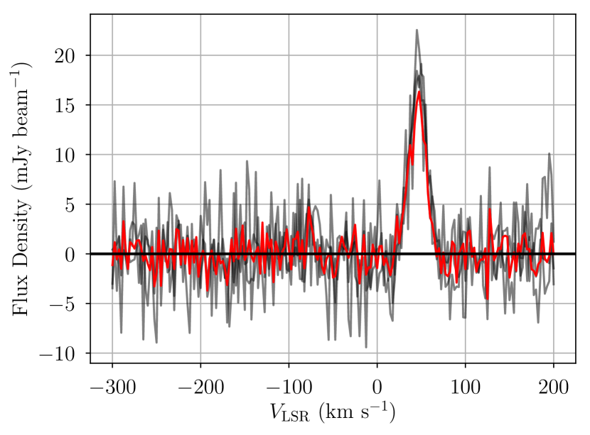
Figure 2: Example SHRDS spectrum showing the spectral sensitivity improvement in the mosaic data. The gray curves are $\langle\text{Hn}\alpha\rangle$ spectra toward G293.994$-$00.934 in three different SHRDS fields. The red curve is the $\langle\text{Hn}\alpha\rangle$ spectrum toward the same source in the mosaic “mos083”. Each spectrum is extracted from the brightest continuum pixel in the smoothed, 4$\,{\rm GHz}$ bandwidth continuum images. The spectral rms is $0.84$, $1.91$, and $1.35\,\text{mJy beam${}^{-1}$}$ in fields “shrds219”, “g293.936$-$”, and “g293.994$-$,” respectively. In the mosaic spectrum, the spectral rms is $0.75\,\text{mJy beam${}^{-1}$}$.

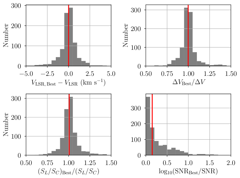
Figure 3: A comparison of the RRL parameters for sources with detections in multiple fields. The top-left panel is the difference between the fitted LSR velocity for the detection with the highest RRL SNR and each other detection of the same source, the top-right panel is the ratio of the fitted FWHM line width, the bottom-left panel is the ratio of the RRL-to-continuum ratios, and the bottom right panel is the ratio of RRL SNR. For nebulae with multiple RRL velocity components, only the brightest RRL component is compared. The median LSR velocity difference is $0.0\,{\rm km\,s^{-1}}$, the median FWHM line width ratio and RRL-to-continuum are both $1.0$, and the median RRL SNR ratio is $1.4$. These median values are indicated by the vertical red line in each panel. Our data analysis techniques recover the same RRL properties for sources detected independently in different fields.

4.2 Radio Recombination Line Catalog

The RRL properties of the SHRDS nebulae are summarized in four different catalogs. The RRL parameters of spectra extracted from the brightest continuum pixel are given in Table 7 (non-smoothed) and Table 8 (smoothed). The RRL parameters derived from the watershed region spectra are given in Table 9 (non-smoothed) and Table 10 (smoothed). For each source, we list the WISE Catalog name and field name. Then, for each RRL transition and $\langle\text{Hn}\alpha\rangle$ spectrum, we list the RRL transition or range of averaged RRLs, RRL rest frequency or weighted-average RRL rest frequency, $\nu$, the velocity component identifier, fitted Gaussian peak RRL brightness or flux density, $S_{L}$, fitted center LSR velocity, $V_{\rm LSR}$, fitted full-width at half-maximum (FWHM) line width, $\Delta V$, continuum brightness or flux density, $S_{C}$, and signal-to-noise ratio, SNR. The average RRL ranges only include those transitions for which there are individual transitions listed in the tables (for example, H90 is not observed and not listed in the table, therefore the “H88-H112” average RRL does not include H90). The average rest frequencies are weighted using the same weights as the $\langle\text{Hn}\alpha\rangle$ spectra (see Equation 4 in Wenger et al. (2019a)). We fit multiple Gaussian components in some cases, and the velocity component identifier is “a” for the brightest component, “b” for the second brightest, etc. The continuum brightness or flux density is the median value of the line-free channels, and the uncertainty is the spectral rms. The SNR is estimated following Lenz & Ayres (1992),

$$SNR=0.7\left(\frac{S_{L}}{\rm rms}\right)\left(\frac{\Delta V}{\Delta v}\right)^{0.5},$$ (2)

where rms is the spectral rms and $\Delta v$ is the channel width.

To test the reproducibility of our RRL catalog, we use the $\langle\text{Hn}\alpha\rangle$ RRL parameters of nebulae with multiple detections. A WISE Catalog source can appear in the RRL tables several times if it is detected in multiple fields and/or mosaics. For example, Figure 2 shows four $\langle\text{Hn}\alpha\rangle$ spectra toward G293.994$-$00.934. The spectrum extracted from the mosaic data has the best sensitivity, as expected. For each source, we identify the RRL detection with the highest SNR (the “best” detection). Figure 3 shows distributions of the differences between the best detections and every other detection for various RRL parameters. Shown are the difference between the LSR velocities, the ratio of FWHM linewidths, the ratio of RRL-to-continuum brightness ratios, and the ratio of RRL SNRs. We only include the brightest RRL component if the source has multiple velocity components. For an optically thin nebula in local thermodynamic equilibrium (LTE), the RRL-to-continuum ratio, $S_{L}/S_{C}$, scales as $S_{L}/S_{C}\propto\nu^{1.1}$, where $\nu$ is the RRL rest frequency (Wenger et al., 2019a). We scale each RRL-to-continuum brightness ratio to 9$\,{\rm GHz}$. The median velocity difference is $0.0\,{\rm km\,s^{-1}}$, and the median ratio of line widths and RRL-to-continuum ratios are both $1.0$. We therefore conclude that our data reduction and analysis procedures are recovering the same RRL properties for multiple detections.

5 Properties of SHRDS Nebulae

The current census of known H ii regions in the WISE Catalog is comprised of 2376 nebulae. This population is the sum of H ii regions discovered by the HRDS and SHRDS, together with those previously known nebulae listed in the WISE Catalog. The HRDS and SHRDS together have discovered ${\sim}1400$ nebulae, more than doubling the WISE Catalog population of Milky Way H ii regions. The SHRDS adds 436 nebulae to this census, a 130% increase in the range $259^{\circ}<\ell<346^{\circ}$. Here we compare the properties of the SHRDS nebulae which the current H ii region census.

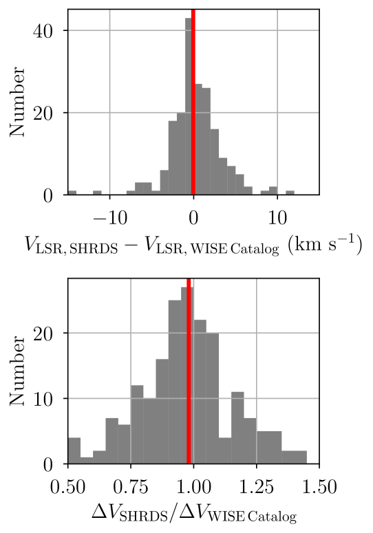
Figure 4: A comparison between the SHRDS RRL parameters and those previously measured for 207 H ii regions. The top panel is the distribution of the difference between the SHRDS LSR velocity, $V_{\rm LSR}$, and the previously measured LSR velocity from the WISE Catalog. The bottom panel is the distribution of the ratio of the SHRDS FWHM line width, $\Delta V$, to the previously measured line width. The red lines indicate the median of each distribution: $0.0\,{\rm km\,s^{-1}}$ (top) and $0.98$ (bottom). For nebulae with multiple RRL velocity components, only the brightest RRL component is compared. We exclude nine nebulae with LSR velocity differences greater than $10\,{\rm km\,s^{-1}}$. The FWHM line width dispersion may stem from the ATCA probing a different volume of gas than the single dish observations.

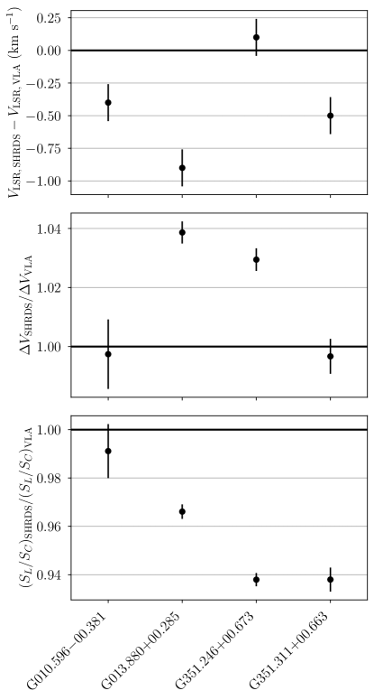
Figure 5: A comparison between the SHRDS RRL and radio continuum data and those previously measured by the VLA (Wenger et al., 2019a) for the four nebulae in common between the two surveys. The top panel is the difference between the SHRDS and VLA RRL LSR velocity, $V_{\rm LSR}$. The middle panel is the ratio of the SHRDS RRL FWHM line width, $\Delta V$, to that measured by the VLA. The bottom panel is the ratio of the RRL-to-continuum brightness ratio, $S_{L}/S_{C}$, measured by the SHRDS to that measured by the VLA. The error bars represent the $1\sigma$ uncertainties, and the horizontal lines represent parity between the two datasets. There is a systematic discrepancy between the SHRDS and VLA RRL-to-continuum brightness ratios.

5.1 Previously Known Nebulae

The SHRDS RRL catalog includes 206 detections toward previously known H ii regions. The total flux density measurements of these nebulae will vary between experiments due to differences in observing frequency, beam size, and the loss of flux in interferometric observations. We can nonetheless use the SHRDS detections of previously known H ii regions to assess the efficacy of the experiment by comparing the kinematic RRL properties (i.e., center velocities and line widths) and RRL-to-continuum brightness ratios.

We find that there are no systematic discrepancies between the SHRDS RRL LSR velocities and FWHM line widths compared to previous single dish measurements. A nebula’s RRL LSR velocity and FWHM line width should be independent of the telescope if each telescope is seeing the same volume of emitting gas. Therefore, we expect to see some differences between the SHRDS RRL parameters and those previously measured by single dish telescopes because the ATCA probes a smaller and more compact volume. Figure 4 compares the LSR velocities and FWHM line widths from the SHRDS against previous single dish measurements listed in the WISE Catalog. We use the SHRDS detection with the highest RRL SNR to make this comparison. There are nine nebulae with LSR velocity differences greater than $10\,{\rm km\,s^{-1}}$: seven from Caswell & Haynes (1987), one from Lockman (1989), and one from Anderson et al. (2011). These outliers are likely due to misassociations with WISE Catalog objects due to the poor angular resolution of the previous studies or confusion in the SHRDS. Excluding these outliers, the median difference between the SHRDS and WISE Catalog RRL LSR velocities is $0.0\,{\rm km\,s^{-1}}$ with a standard deviation of $2.7\,{\rm km\,s^{-1}}$. In contrast, the median FWHM line width ratio is $0.98$ with a standard deviation of $0.23$. These distributions are consistent with no systematic difference between the SHRDS and single dish studies. The large dispersion of the FWHM line width distribution, however, supports our expectation that the ATCA is probing a different volume of gas.

Although we find no systematic differences between the SHRDS and previous single dish measurements, we do find some discrepancies compared to previous interferometric observations with the VLA. There are four nebulae observed in both the SHRDS and the Wenger et al. (2019a) VLA survey: G010.596$-$00.381, G013.880+00.285, G351.246+00.673, and G351.311+00.663. All four nebulae are robust detections with a RRL SNR $>100$ in both surveys. Overall they also have excellent continuum data with QF A in both surveys, except for G010.596$-$00.381 with QF C in the SHRDS. The differences between the SHRDS and VLA RRL LSR velocities and FWHM line widths are small (see top two panels of Figure 5). The median LSR velocity difference and FWHM line width ratio are $-0.5\,{\rm km\,s^{-1}}$ and $1.01$, respectively. The bottom panel of Figure 5 shows the ratio of the SHRDS and VLA RRL-to-continuum ratios after scaling each to a 8$\,{\rm GHz}$. Here there is a systematic discrepency between the two surveys; the median SHRDS RRL-to-continuum ratio is 95% of the VLA ratio. These differences may be a consequence of the much larger synthesized beam size in the SHRDS (${\sim}100{{{}^{\prime\prime}}}$) probing a larger volume of gas compared to the VLA ${\sim}10{{{}^{\prime\prime}}}$, or they may be due to optical depth or non-LTE effects. Since the RRL-to-continuum ratio is used to derive electron temperatures and infer nebular metallicities in Galactic H ii regions, this systematic offset must be investigated further.

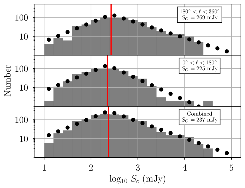
Figure 6: The distribution of GBT HRDS and SHRDS H ii region 9$\,{\rm GHz}$ continuum flux densities. The top panel shows only those nebulae in the third and fourth Galactic quadrants ($180^{\circ}<\ell<360^{\circ}$; $n=728$) and the middle panel shows only those nebulae in the first and second Galactic quadrants ($0^{\circ}<\ell<180^{\circ}$; $n=606$). The bottom panel shows all Galactic H ii regions with GBT HRDS or SHRDS flux density measurements $n=1334$. The black points represent the expected population in each bin from the maximum likelihood power law distribution (Equation 3). The vertical red lines are the maximum likelihood 9$\,{\rm GHz}$ continuum flux density completeness limits, $S_{C}$, derived for each sample: $269\,\text{mJy}$ (top), $225\,\text{mJy}$ (middle), and $237\,\text{mJy}$ (bottom). This analysis suggests that the Galactic H ii region census is complete to ${\sim}250\,\text{mJy}$.

5.2 H ii Region Census Completeness

We estimate the completeness of the WISE Catalog Galactic H ii region census, including the SHRDS Full Catalog data, by making two assumptions: (1) the Galactic H ii region luminosity function at ${\sim}9\,{\rm GHz}$ is a power law (e.g., Smith & Kennicutt, 1989; McKee & Williams, 1997; Paladini et al., 2009; Mascoop et al., in press), and (2) the nebulae are distributed roughly uniformly across the Galactic disk (see Anderson et al., 2011). Under these assumptions, the observed flux density distribution of Galactic H ii regions should also follow a power law, and we estimate the completeness of the sample as the point where the observed flux density distribution deviates from a power law.

We use a maximum likelihood approach to fit a power law distribution to the continuum flux density distribution. The assumed form of the flux density probability distribution function, $p(S;\beta,S_{c})$, is

$$p(S;\beta,S_{c})=\begin{cases}A\left(\frac{S}{S_{c}}\right)^{-\beta}&S>S_{c}\\ A&S_{m}\leq S<S_{c}\\ 0&S\leq S_{m}\end{cases},$$ (3)

where $S$ is the flux density, $S_{c}$ is the point at which the distribution breaks from a power law, $S_{m}$ is the minimum observed flux density, and $A$ is a normalization constant given by

$$A=\frac{\beta-1}{\beta(S_{c}-S_{m})+S_{m}}.$$ (4)

Figure 6 shows the distribution of continuum flux densities for Galactic H ii regions with GBT HRDS or SHRDS continuum flux density measurements in three Galactic longitude zones. The top panel is the third and fourth Galactic quadrants ($180^{\circ}<\ell<360^{\circ}$), which includes the majority of the SHRDS sources. The middle panel is the first and second quadrants ($0^{\circ}<\ell<180^{\circ}$), which contains the majority of the HRDS nebulae as well as 12 SHRDS detections. The bottom panel is the whole Galaxy. Assuming the nebulae are optically thin, we use a thermal spectral index, $\alpha=-0.1$, to scale all flux densities to $9\,{\rm GHz}$. The GBT HRDS did not observe previously known nebulae. Therefore, the middle panel in Figure 6 has an obvious lack of bright nebulae.

Under these assumptions, we estimate that the WISE Catalog Galactic H ii region census is complete to a $9\,{\rm GHz}$ continuum flux density limit of ${\sim}250\,\text{mJy}$. This flux density corresponds to the brightness of an H ii region ionized by a single O9 V star at $10\,\text{kpc}$ (Anderson et al., 2011). To derive this completeness estimate, we generate 10,000 Monte Carlo realizations of the H ii region data by resampling the continuum flux densities within their uncertainties. We fit the broken power law distribution (Equation 3) to each realization. The median values of the power law breaks, $S_{c}$, are $269\,\text{mJy}$ ($180^{\circ}<\ell<360^{\circ}$), $225\,\text{mJy}$ ($0^{\circ}<\ell<180^{\circ}$), and $237\,\text{mJy}$ (combined). Assuming that the power law breaks represent the completeness of each sample, then the completeness in the third and fourth quadrants is ${\sim}15\%$ worse than that of the first and second quadrants. There are at least three important limitations to our completeness analysis. First, the GBT continuum flux density measurements may be inaccurate (see Wenger et al., 2019a). Second, the assumption of a homogeneous distribution of H ii regions across the Galactic disk is a simplified approximation (see the following section). Third, the SHRDS continuum flux densities may be underestimated due to missing flux.

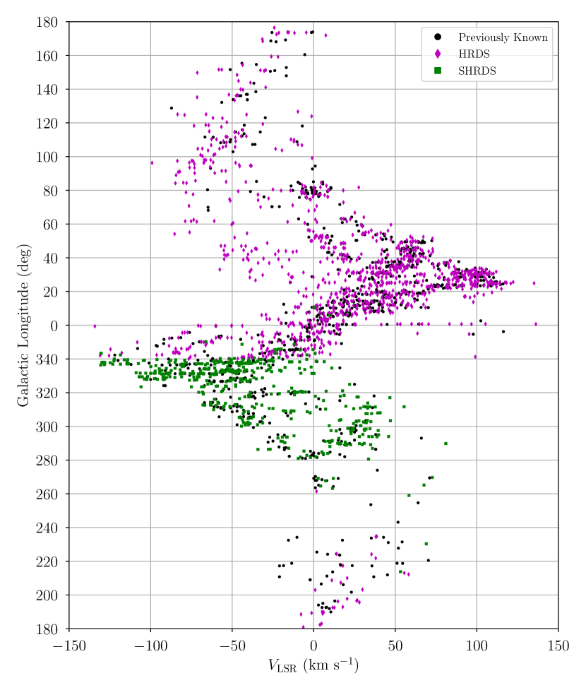
Figure 7: Galactic longitude, $\ell$, and LSR velocity, $V_{\rm LSR}$, for all known Galactic H ii regions in the WISE Catalog with $|V_{\rm LSR}|<150\,{\rm km\,s^{-1}}$. Including the ${\sim}40$ nebulae outside of this velocity range, there are 2376 known Galactic H ii regions: 961 previously known nebulae from the WISE Catalog (black points), 979 GBT and Arecibo HRDS nebulae (magenta diamonds), and 436 SHRDS nebulae (green squares). Some nebulae have multiple ionized gas velocity components; we include one data point for each component.

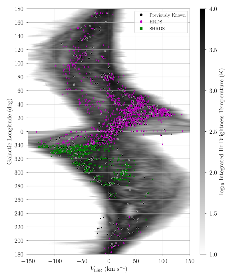
Figure 8: Same as Figure 7, plotted atop the HI4PI Collaboration et al. (2016) H i brightness temperature integrated over $|b|<2^{\circ}$.

5.3 Southern vs. Northern Nebulae

The simplest model for the distribution of Galactic H ii regions is a population of nebulae distributed homogeneously across the Milky Way’s disk. This is our null-hypothesis and a useful starting point for future explorations of more complicated models. Given a homogeneous H ii region distribution and axisymmetric Galactic rotation, one would expect a symmetric Galactic longtidue-velocity ($\ell$-$v$) distribution of H ii regions between the northern and southern skies. For the first time, we use a complete census of Galactic H ii regions across the entire sky to test whether such global symmetry exists. Figure 7 shows the $\ell$-$v$ distribution of all known Galactic H ii regions in the WISE Catalog, including those discovered in the SHRDS. Figure 8 shows the same information plotted atop a grey scale image of the distribution of 21 cm H i emission (HI4PI Collaboration et al., 2016).

Table 11: Galactic H ii Region Census Properties

Property	First Quadrant	Second Quadrant	Third Quadrant	Fourth Quadrant	Entire Galaxy
	($0^{\circ}<\ell<90^{\circ}$)	($90^{\circ}<\ell<180^{\circ}$)	($180^{\circ}<\ell<270^{\circ}$)	($270^{\circ}<\ell<360^{\circ}$)	($0^{\circ}<\ell<360^{\circ}$)
Number of H ii Regions	1176	155	90	955	2376
9$\,{\rm GHz}$ Continuum Completeness (mJy)	269		225		237
Median LSR Velocity ($\,{\rm km\,s^{-1}}$)	$39.8$	$-47.9$	$11.6$	$-38.0$	$5.0$
LSR Velocity Std. Dev. ($\,{\rm km\,s^{-1}}$)	$39.4$	$21.8$	$21.9$	$45.0$	$54.9$
Median RRL FWHM Line Width ($\,{\rm km\,s^{-1}}$)	$23.7$	$24.6$	$24.1$	$23.9$	$23.9$
RRL FWHM Line Width Std. Dev. ($\,{\rm km\,s^{-1}}$)	$6.7$	$5.5$	$7.6$	$7.0$	$6.8$

The asymmetry in the H ii region $\ell$-$v$ distribution between the northern and southern sky is striking. This H ii region asymmetry is contrasted by the H i symmetry in Figure 8. H i is ubiquitous in the Milky Way (e.g., Kalberla & Kerp, 2009) and thus symmetrically fills all space in the $\ell$-$v$ plane allowed by Galactic rotation. In contrast, Galactic H ii regions are neither ubiquitous nor are they distributed homogeneously. They do not populate the same $\ell$-$v$ space as the neutral gas and their $\ell$-$v$ distribution is asymmetric between the northern (first and second quadrants) and southern (third and fourth quadrants) sky. Table 11 lists the properties of the Galactic H ii region census in each Galactic quadrant. There are more H ii regions in the northern sky ($n=1331$) compared with the southern sky ($n=1045$). Furthermore, the asymmetry extends to the inner vs. outer Galaxy. The ratio of known H ii regions in the fourth quadrant to the first quadrant is 81% whereas the ratio of third quadrant to second quadrant nebulae is only 58%.

A similar asymmetry is seen in the distribution of WISE Catalog H ii regions and H ii region candidates (Anderson et al., 2014). This asymmetry cannot be fully explained by completeness differences between these Galactic zones. The current Galactic H ii region census has 315 third and fourth quadrant nebulae with 9$\,{\rm GHz}$ continuum flux densities less than the southern sky completeness limit, 269 mJy. If this sample was complete to the northern sky limit, 225 mJy, then we would expect to find an additional 54 southern sky nebulae. The current H ii region census has 286 more northern sky nebulae than southern sky nebulae. This difference is ${\sim}5.3$ times greater than what can be explained by the completeness disparity. The global Galactic asymmetry in the distribution of the formation sites of massive stars probably stems from spiral structure.

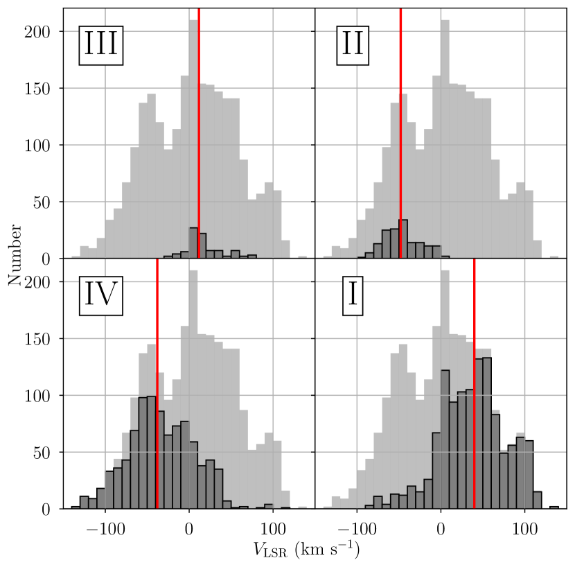
Figure 9: The distribution of WISE Catalog H ii region RRL LSR velocities, $V_{\rm LSR}$, in each of the Galactic quadrants. The median LSR velocities (number of nebulae) are $39.8\,{\rm km\,s^{-1}}$ (1176), $-47.9\,{\rm km\,s^{-1}}$ (155), $11.6\,{\rm km\,s^{-1}}$ (90), and $-38.0\,{\rm km\,s^{-1}}$ (955) in the first, second, third, and fourth quadrants, respectively. These median values are indicated by the vertical red lines in each panel. The background histrograms show the distribution of RRL LSR velocities for the full census of Galactic H ii regions in the WISE Catalog. For nebulae with multiple RRL velocity components, only the brightest RRL component is included. There is an asymmetry in the H ii region LSR velocity distribution between the northern and southern sky.

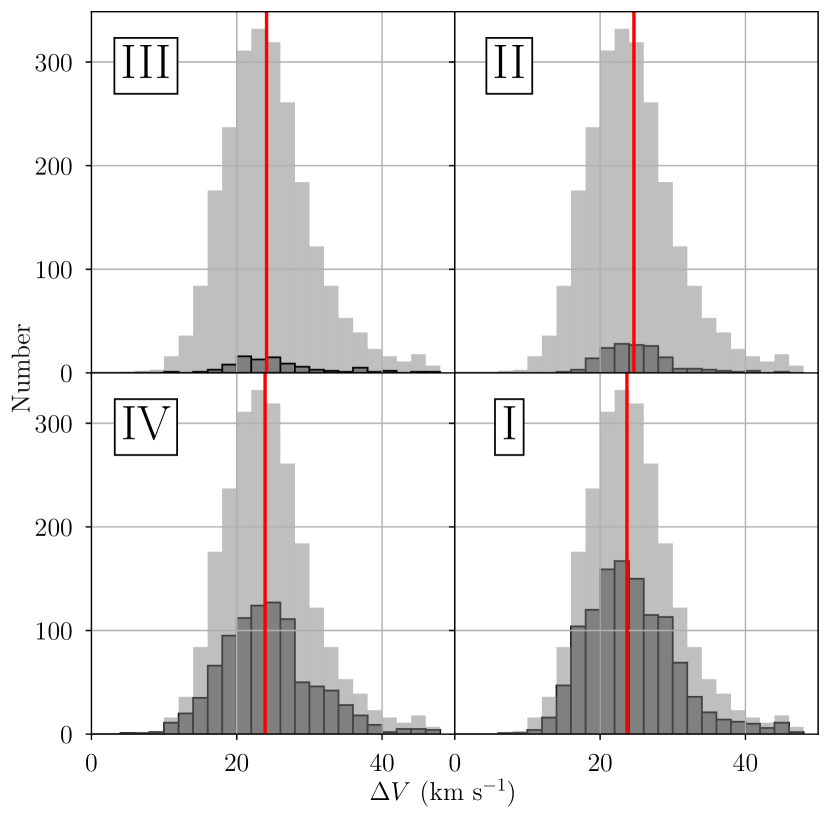
Figure 10: The distribution of WISE Catalog H ii region RRL FWHM line widths, $\Delta V$, in each of the Galactic quadrants. The median FWHM line widths are $23.7\,{\rm km\,s^{-1}}$, $24.6\,{\rm km\,s^{-1}}$, $24.1\,{\rm km\,s^{-1}}$, and $23.9\,{\rm km\,s^{-1}}$ in the first, second, third, and fourth quadrants, respectively. These median values are indicated by the vertical red lines in each panel. The median FHWM line width of the entire population is $23.9\,{\rm km\,s^{-1}}$. The background histrograms show the distribution of RRL FWHM line widths for the full census of Galactic H ii regions in the WISE Catalog. For nebulae with multiple RRL velocity components, only the brightest RRL component is included. There is no evidence that H ii region RRL line widths depend on Galactic location.

The Figure 7 $\ell$-$v$ diagram also reveals an asymmetry in the H ii region velocity distribution. In the third and fourth quadrants, for example, there are few nebulae with $V_{\rm LSR}>50\,{\rm km\,s^{-1}}$. In comparison, the symmetric region of the first and second quadrants, $V_{\rm LSR}<-50\,{\rm km\,s^{-1}}$, is thoroughly populated. To better illustrate this asymmetry, Figure 9 shows the distribution of H ii region LSR velocities in each Galactic quadrant. The median and standard deviation of each distribution is listed in Table 11. Over the entire Galaxy, the median H ii region LSR velocity is $5.0\,{\rm km\,s^{-1}}$ with a standard deviation of $54.9\,{\rm km\,s^{-1}}$.

The first and fourth quadrant distributions are symmetric; the magnitudes of their median LSR velocities are within $2\,{\rm km\,s^{-1}}$ and the widths of the distributions are comparable to within 15%. The median velocities, however, are not symmetric between the second and third quadrants. The second and third quadrants also have similar LSR velocity distribution widths, although they are ${\sim}50\%$ narrower than the first and fourth quadrant distributions. Such asymmetry is not expected for a homogeneous and axisymmetric distribution of H ii regions. This velocity asymmetry is probably an artifact of spiral structure in the H ii region distribution.

The RRL FWHM linewidth distribution of the southern sky nebulae is nearly indistinguishable from the northern sky population. Figure 10 shows the distribution of RRL FWHM linewidths in each of the Galactic quadrants. The median and standard deviation of each distribution is listed in Table 11. The median RRL FWHM linewidth of all known Galactic H ii regions in the WISE Catalog, including the new SHRDS nebulae, is $23.9\,{\rm km\,s^{-1}}$ with a standard deviation of $6.8\,{\rm km\,s^{-1}}$. Such uniformity of these distributions implies that the physical conditions of H ii regions (e.g., internal turbulence) must be similar across the Galaxy.

6 Completing the Census of Galactic H ii Regions

With this data release, we conclude our H ii Region Discovery Surveys, which began with the GBT HRDS nearly a decade ago. The SHRDS Full Catalog data are included both in the latest release of the WISE Catalog of Galactic H ii Regions (Anderson et al., 2014) and in a machine-readable database of ionized gas detections toward Galactic H ii regions. The WISE Catalog now contains 2376 known H ii regions, 1690 candidates, 3718 radio-quiet candidates, and 632 group candidates. The H ii region census is complete to ${\sim}250$ mJy at 9$\,{\rm GHz}$. The remaining H ii region candidates are likely distant or ionized by lower mass stars (Armentrout et al., 2021).

With ${\sim}6000$ remaining H ii region candidates in the WISE catalog, the census of Galactic H ii regions is still incomplete. New single dish RRL surveys in search of new Galactic H ii regions must be mindful that poor angular resolution complicates the interpretation of the source of the emission. For example, Chen et al. (2020) claim the detection of RRL emission in ${\sim}75$ directions not associated with a WISE Catalog object. An inspection of these positions reveals that many are overlapping or immediately adjacent to one or more WISE Catalog sources. The source of the detected RRL emission could therefore be the H ii region itself, ionized gas in the immediate vicinity of the H ii region due to leaked ionizing photons (e.g., Luisi et al., 2016), or diffuse ionized gas (DIG) somewhere along the line of sight (e.g., Liu et al., 2019). As we push to better sensitivity in single dish surveys, it will become more challenging to disentangle RRL emission toward discrete sources from the DIG.

To complete the census of Galactic H ii regions and find RRL emission toward the remaining WISE Catalog candidates, the next generation of H ii region discovery surveys will require better sensitivity. A nebula ionized by a single B0 V star 25 kpc distant, for example, has a 9$\,{\rm GHz}$ continuum flux density of ${\sim}10\,\text{mJy}$ (Anderson et al., 2011; Armentrout et al., 2021; Mascoop et al., in press). Assuming a typical RRL-to-continuum ratio of $0.1$ at $9\,{\rm GHz}$, the RRL flux density is ${\sim}1\,\text{mJy}$. The VLA would require an on-source integration time of ${\sim}30\,\text{min}$ ($560\,\text{min}$ for the ATCA) to achieve a $5\sigma$ RRL detection in $5\,{\rm km\,s^{-1}}$ channels after averaging 8 RRL transitions. These integration times are impracticable for a survey of several thousand H ii region candidates. Future facilities, such as the Next Generation Very Large Array (ngVLA) and Square Kilometer Array (SKA) will be capable of finding RRLs toward most, if not all, of the remaining Galactic H ii region candidates. The angular resolution of these instruments will also allow for the extinction-free detection of discrete H ii regions in nearby galaxies (Balser et al., 2018).

7 Summary

The SHRDS comprises the final contribution to our H ii Region Discovery Surveys. With the ATCA, we detect 4–10$\,{\rm GHz}$ radio continuum emission toward 212 previously known H ii regions and 518 H ii region candidates. We detect RRL emission toward 208 previously known nebulae and 438 H ii region candidates by averaging ${\sim}18$ RRL transitions. The detection of RRL emission from these nebulae thus increases the number of known WISE Catalog Galactic H ii regions in the surveyed zone by 130% to 778 nebulae. Including the previous northern sky surveys with the GBT and Arecibo Telescope, as well as the SHRDS, the HRDS has now discovered ${\sim}1400$ new nebulae. These discoveries made during the past decade have more than doubled the number of known Galactic H ii regions in the WISE Catalog.

All SHRDS data products, including continuum images and data cubes for each RRL transition, are publicly available. These data are included both in the latest release of the WISE Catalog of Galactic H ii Regions (Anderson et al., 2014) and in a machine-readable database. A single nebula may appear multiple times in our radio continuum and RRL catalogs because we analyze the data in several different ways. For example, a source may be detected in both the non-smoothed and smoothed images. For each detected nebula we measure both the peak and total continuum flux density. We determine the RRL properties in spectra extracted from the brightest pixel as well as in spectra averaged over all pixels containing emisssion. Furthermore, a nebula may be detected in multiple individual fields or mosaics. Users of these catalogs should use the data that best fit their science goals.

The census of Galactic H ii regions in the WISE Catalog is now complete to ${\sim}250\,\text{mJy}$ at $9\,{\rm GHz}$. This flux density is equivalent to a nebula ionized by a single O9 V star at a distance of ${\sim}10\,\text{kpc}$. The distribution of H ii region RRL line widths is similar in each Galactic quadrant, with a median FWHM line width of $23.9\,{\rm km\,s^{-1}}$. The asymmetry in the number of nebulae and the distributions of RRL LSR velocities probably stems from Galactic spiral structure.

With a flux-limited sample of nebulae across the Milky Way, we can now begin to craft a comprehensive view of Galactic chemical and morphological structure. A face-on map of the H ii region locations requires accurate distances, which can be derived from maser parallax measurements (e.g., Reid et al., 2019) or kinematically (e.g., Wenger et al., 2018). In an upcoming paper in this series, we will use H i absorption observations to resolve the kinematic distance ambiguity and thus derive the distances to hundreds of SHRDS nebulae.

The next generation of Galactic H ii region discovery surveys will require the sensitivity of future facilities, such as the ngVLA and the SKA. These telescopes will have the sensitivity to detect continuum and RRL emission toward most Galactic H ii regions as well as the angular resolution to resolve the emission from discrete H ii regions in nearby galaxies. Such extragalactic studies will not only provide an extinction-free tracer of star formation in these galaxies, but also a direct comparison to what we are learning about Milky Way high-mass star formation, Galactic chemical structure, and Galactic morphological structure.

Appendix A Sinc Interpolation

Sinc interpolation provides a perfect reconstruction of discrete signals sampled at the Nyquist rate or higher (Oppenheim et al., 1975). It is the proper way to interpolate time-limited (or band-limited), discrete frequency (or time) signals to arbitrary frequencies (or times) and/or sampling rates. For an original spectrum, $s(v)$, sampled at velocities, $v_{0},v_{1},...,v_{N}$, the smoothed and re-sampled spectrum, $s^{*}(v^{*})$, sampled at velocities, $v^{*}_{0},v^{*}_{1},...,v^{*}_{M}$, with channel spacing $\Delta v^{*}$ is the linear convolution of $s(v)$ with a sinc function,

$$s^{*}(v^{*}_{j})=\sum_{i}^{N}s(v_{i})A_{j}\,\text{sinc}\left(\frac{v^{*}_{j}-v_{i}}{\Delta v^{*}}\right),$$ (A1)

where $A_{j}$ is a normalization constant such that

$$\sum_{i}^{N}A_{j}\,\text{sinc}\left(\frac{v^{*}-v_{i}}{\Delta v^{*}}\right)=1,$$ (A2)

and $\text{sinc}(x)=\sin(\pi x)/(\pi x)$.

Smoothing and interpolating large data cubes is implemented efficiently by treating the convolution as a tensor dot product. For a multi-dimensional data cube $\boldsymbol{S}$ with the $N$-length velocity axis along the first dimension (e.g., a four-dimensional data cube with the typical radio astronomy axes: velocity, Galactic latitude, Galactic longitude, and Stokes), the smoothed data cube with the $M$-length re-gridded velocity axis along the first dimension is the tensor dot product,

$$\boldsymbol{S}^{*}=\boldsymbol{W}\cdot\boldsymbol{S},$$ (A3)

where $\boldsymbol{W}$ is the $M\times N$ array of sinc weights with elements

$$w_{ij}=A_{j}\,\text{sinc}\left(\frac{v^{*}_{j}-v_{i}}{\Delta v^{*}}\right).$$ (A4)

References

- Anderson et al. (2015) Anderson, L. D., Armentrout, W. P., Johnstone, B. M., et al. 2015, ApJS, 221, 26, doi: 10.1088/0067-0049/221/2/26
- Anderson et al. (2018) Anderson, L. D., Armentrout, W. P., Luisi, M., et al. 2018, ApJS, 234, 33, doi: 10.3847/1538-4365/aa956a
- Anderson et al. (2014) Anderson, L. D., Bania, T. M., Balser, D. S., et al. 2014, ApJS, 212, 1, doi: 10.1088/0067-0049/212/1/1
- Anderson et al. (2011) Anderson, L. D., Bania, T. M., Balser, D. S., & Rood, R. T. 2011, ApJS, 194, 32, doi: 10.1088/0067-0049/194/2/32
- Anderson et al. (2012) —. 2012, ApJ, 754, 62, doi: 10.1088/0004-637X/754/1/62
- Armentrout et al. (2021) Armentrout, W. P., Anderson, L. D., Wenger, T. V., Balser, D. S., & Bania, T. M. 2021, ApJS, 253, 23, doi: 10.3847/1538-4365/abd5c0
- Astropy Collaboration et al. (2013) Astropy Collaboration, Robitaille, T. P., Tollerud, E. J., et al. 2013, A&A, 558, A33, doi: 10.1051/0004-6361/201322068
- Balser et al. (2018) Balser, D. S., Anderson, L. D., Bania, T. M., et al. 2018, in Astronomical Society of the Pacific Conference Series, Vol. 517, Science with a Next Generation Very Large Array, ed. E. Murphy, 431
- Balser et al. (2011) Balser, D. S., Rood, R. T., Bania, T. M., & Anderson, L. D. 2011, ApJ, 738, 27, doi: 10.1088/0004-637X/738/1/27
- Bania et al. (2012) Bania, T. M., Anderson, L. D., & Balser, D. S. 2012, ApJ, 759, 96, doi: 10.1088/0004-637X/759/2/96
- Bania et al. (2010) Bania, T. M., Anderson, L. D., Balser, D. S., & Rood, R. T. 2010, ApJ, 718, L106, doi: 10.1088/2041-8205/718/2/L106
- Becker et al. (1994) Becker, R. H., White, R. L., Helfand, D. J., & Zoonematkermani, S. 1994, ApJS, 91, 347, doi: 10.1086/191941
- Bertrand (2005) Bertrand, G. 2005, Journal of Mathematical Imaging and Vision, 22, 217, doi: 10.1007/s10851-005-4891-5
- Brown et al. (2017) Brown, C., Jordan, C., Dickey, J. M., et al. 2017, AJ, 154, 23, doi: 10.3847/1538-3881/aa71a7
- Caswell & Haynes (1987) Caswell, J. L., & Haynes, R. F. 1987, A&A, 171, 261
- Chen et al. (2020) Chen, H.-Y., Chen, X., Wang, J.-Z., Shen, Z.-Q., & Yang, K. 2020, ApJS, 248, 3, doi: 10.3847/1538-4365/ab818e
- Churchwell (2002) Churchwell, E. 2002, ARA&A, 40, 27, doi: 10.1146/annurev.astro.40.060401.093845
- Cornwell et al. (1993) Cornwell, T. J., Holdaway, M. A., & Uson, J. M. 1993, A&A, 271, 697
- Downes et al. (1980) Downes, D., Wilson, T. L., Bieging, J., & Wink, J. 1980, A&AS, 40, 379
- Gum (1955) Gum, C. S. 1955, MmRAS, 67, 155
- HI4PI Collaboration et al. (2016) HI4PI Collaboration, Ben Bekhti, N., Flöer, L., et al. 2016, A&A, 594, A116, doi: 10.1051/0004-6361/201629178
- Hoglund & Mezger (1965a) Hoglund, B., & Mezger, P. G. 1965a, Science, 150, 339, doi: 10.1126/science.150.3694.339
- Hoglund & Mezger (1965b) —. 1965b, AJ, 70, 678
- Hunter (2007) Hunter, J. D. 2007, Computing In Science & Engineering, 9, 90, doi: 10.1109/MCSE.2007.55
- Kalberla & Kerp (2009) Kalberla, P. M. W., & Kerp, J. 2009, ARA&A, 47, 27, doi: 10.1146/annurev-astro-082708-101823
- Kardashev (1959) Kardashev, N. S. 1959, Soviet Ast., 3, 813
- Lenz & Ayres (1992) Lenz, D. D., & Ayres, T. R. 1992, PASP, 104, 1104, doi: 10.1086/133096
- Leto et al. (2009) Leto, P., Umana, G., Trigilio, C., et al. 2009, A&A, 507, 1467, doi: 10.1051/0004-6361/200911894
- Liu et al. (2019) Liu, B., Anderson, L. D., McIntyre, T., et al. 2019, ApJS, 240, 14, doi: 10.3847/1538-4365/aaef8e
- Lockman (1989) Lockman, F. J. 1989, ApJS, 71, 469, doi: 10.1086/191383
- Lockman et al. (1996) Lockman, F. J., Pisano, D. J., & Howard, G. J. 1996, ApJ, 472, 173, doi: 10.1086/178052
- Luisi et al. (2016) Luisi, M., Anderson, L. D., Balser, D. S., Bania, T. M., & Wenger, T. V. 2016, ApJ, 824, 125, doi: 10.3847/0004-637X/824/2/125
- Mascoop et al. (in press) Mascoop, J. L., Anderson, L. D., Makai, Z., et al. in press, ApJ
- McKee & Williams (1997) McKee, C. F., & Williams, J. P. 1997, ApJ, 476, 144, doi: 10.1086/303587
- McMullin et al. (2007) McMullin, J. P., Waters, B., Schiebel, D., Young, W., & Golap, K. 2007, in Astronomical Society of the Pacific Conference Series, Vol. 376, Astronomical Data Analysis Software and Systems XVI, ed. R. A. Shaw, F. Hill, & D. J. Bell, 127
- Oppenheim et al. (1975) Oppenheim, A., Schafer, R., of Technology. Center for Advanced Engineering Study, M. I., of Electrical, I., & Board, E. E. E. A. 1975, Digital Signal Processing, MIT video course (Prentice-Hall)
- Paladini et al. (2009) Paladini, R., De Zotti, G., Noriega-Crespo, A., & Carey, S. J. 2009, ApJ, 702, 1036, doi: 10.1088/0004-637X/702/2/1036
- Quireza et al. (2006) Quireza, C., Rood, R. T., Balser, D. S., & Bania, T. M. 2006, ApJS, 165, 338, doi: 10.1086/503901
- Reid et al. (2019) Reid, M. J., Menten, K. M., Brunthaler, A., et al. 2019, ApJ, 885, 131, doi: 10.3847/1538-4357/ab4a11
- Reifenstein et al. (1970) Reifenstein, E. C., Wilson, T. L., Burke, B. F., Mezger, P. G., & Altenhoff, W. J. 1970, A&A, 4, 357
- Rodgers et al. (1960) Rodgers, A. W., Campbell, C. T., & Whiteoak, J. B. 1960, MNRAS, 121, 103, doi: 10.1093/mnras/121.1.103
- Sewilo et al. (2004) Sewilo, M., Churchwell, E., Kurtz, S., Goss, W. M., & Hofner, P. 2004, ApJ, 605, 285, doi: 10.1086/382268
- Sharpless (1953) Sharpless, S. 1953, ApJ, 118, 362, doi: 10.1086/145765
- Sharpless (1959) —. 1959, ApJS, 4, 257, doi: 10.1086/190049
- Smith & Kennicutt (1989) Smith, T. R., & Kennicutt, Jr., R. C. 1989, PASP, 101, 649, doi: 10.1086/132481
- van der Walt et al. (2011) van der Walt, S., Colbert, S. C., & Varoquaux, G. 2011, Computing in Science & Engineering, 13, 22, doi: 10.1109/MCSE.2011.37
- Wenger (2018) Wenger, T. V. 2018, Astrophysics Source Code Library
- Wenger et al. (2018) Wenger, T. V., Balser, D. S., Anderson, L. D., & Bania, T. M. 2018, ApJ, 856, 52, doi: 10.3847/1538-4357/aaaec8
- Wenger et al. (2019a) —. 2019a, ApJ, 887, 114, doi: 10.3847/1538-4357/ab53d3
- Wenger et al. (2013) Wenger, T. V., Bania, T. M., Balser, D. S., & Anderson, L. D. 2013, ApJ, 764, 34, doi: 10.1088/0004-637X/764/1/34
- Wenger et al. (2019b) Wenger, T. V., Dickey, J. M., Jordan, C. H., et al. 2019b, ApJS, 240, 24, doi: 10.3847/1538-4365/aaf8ba
- White et al. (1991) White, R. L., Becker, R. H., & Helfand, D. J. 1991, ApJ, 371, 148, doi: 10.1086/169879
- Wilner & Welch (1994) Wilner, D. J., & Welch, W. J. 1994, ApJ, 427, 898, doi: 10.1086/174195
- Wilson et al. (1970) Wilson, T. L., Mezger, P. G., Gardner, F. F., & Milne, D. K. 1970, A&A, 6, 364
- Wood & Churchwell (1989) Wood, D. O. S., & Churchwell, E. 1989, ApJ, 340, 265, doi: 10.1086/167390
- Wright et al. (2010) Wright, E. L., Eisenhardt, P. R. M., Mainzer, A. K., et al. 2010, AJ, 140, 1868, doi: 10.1088/0004-6256/140/6/1868