Gravitational breathing memory and dual symmetries

Abstract

Brans-Dicke theory contains an additional propagating mode which causes homogeneous expansion and contraction of test bodies in transverse directions. This “breathing” mode is associated with novel memory effects in addition to those of general relativity. Standard tensor mode memories are related to a symmetry principle: they are determined by the balance equations corresponding to the BMS symmetries. In this paper, we show that the leading and subleading breathing memory effects are determined by the balance equations associated with the leading and “overleading” asymptotic symmetries of a dual formulation of the scalar field in terms of a two-form gauge field. The memory effect causes a transition in the vacuum of the dual gauge theory. These results highlight the significance of dual charges and the physical role of overleading asymptotic symmetries.

1 Introduction

The gravitational wave (GW) is not purely an oscillatory waveform, but it includes a non-oscillatory part that builds up over time and leads to a final offset in the waveform. This is the so-called GW “memory” effect. When such a waveform passes through a set of test masses which are initially at rest, the GW memory causes a permanent displacement in their relative distances. This “displacement” memory effect is known since the 70’s Zeldovich:1974gvh . However, the early understanding constituted only part of the memory, nowadays known as the linear or ordinary part. It was later realized by Christodoulou Christodoulou:1991cr and independently by Blanchet and Damour Blanchet:1992br that the radiation of massless fields, including GWs, leads to another contribution to the memory which is called the non-linear or null memory. The construction of Christodoulou:1991cr was based on an asymptotic analysis of Einstein equations in asymptotically flat spacetimes. Another outcome of the asymptotic analysis is the appearance of BMS symmetries in asymptotically flat spacetimes Bondi:1962px ; Sachs:1962wk as an infinite dimensional extension of the Poincaré algebra. However, the interplay between the GW memory and BMS symmetries was uncovered only recently Strominger:2014pwa . Indeed, Strominger and collaborators discovered the so-called IR triangle, which displayed the correspondence between three low energy effects in general relativity (GR), namely the BMS group, displacement memory effect, and Weinberg’s soft graviton theorem Strominger:2017zoo . The correspondence also holds at subleading level where the subleading soft graviton theorem is related to an extension of BMS algebra by super Lorentz symmetries Barnich:2010eb ; Campiglia:2014yka ; Campiglia:2015yka . The corresponding memories are called the spin Pasterski:2015tva and center of mass memories Nichols:2018qac .

Similar construction applies to gauge theory Strominger:2017zoo , where the large gauge symmetries play the role of BMS symmetries and the associated memory is a kick effect Bieri:2013hqa ; Pasterski:2015zua . However, a natural puzzle arises for a massless scalar QFT in Minkowski spacetime: which symmetry would be responsible for the soft factorization in this theory? In Campiglia:2017dpg a set of charges were build such that the correspondence holds. It was shown in Campiglia:2018see ; Francia:2018jtb that these charges can be formulated as the Noether charges associated to the asymptotic symmetries of a dual formulation of the theory in terms of two form fields. Asymptotic symmetries and charges of $p$ form gauge theories in four and higher dimensions are studied in Afshar:2018apx (see Esmaeili:2020eua for a review). Indeed, defining charges in a theory by resorting to the symmetries of a dual formulation of the theory is not restricted to massless scalars, but also includes magnetic type charges in Maxwell theory Hosseinzadeh:2018dkh ; Freidel:2018fsk ; Henneaux:2020nxi and gravity Godazgar:2018qpq ; Kol:2019nkc ; Godazgar:2019dkh ; Godazgar:2020kqd ; Oliveri:2020xls .

What is interesting about scalar tensor theories and particularly Brans-Dicke (BD) theory is that the non-minimal coupling between the scalar and the metric leads to an additional gravitational degree of freedom. This transverse scalar mode, leads to homogeneous expansion and contraction of test bodies in the transverse plane of the GW propagation, thus also called the “breathing” mode. More formally, considering a congruence of geodesics subject to GWs, the $+,\times$ modes lead to shearing effects, while the scalar mode causes an expansion in the evolution of the congruence. Accordingly, BD theory has an additional breathing memory on top of the usual memories present in GR. The breathing memory was first found by Lang Lang:2013fna ; Lang:2014osa and some of its observational aspects are investigated in Du:2016hww ; Koyama:2020vfc . Recently, Tahura et al. Tahura:2020vsa found a “subleading” breathing memory effect in BD theory by considering the congruence of timelike geodesics with initial relative velocity.

The BMS symmetries and their balance equations in BD theory were studied in detail in Hou:2020wbo ; Tahura:2020vsa ; Hou:2020tnd . These balance equations determine the memory effects in tensorial modes of the GW. However, the additional breathing memories in BD theory, have no obvious symmetry counterpart, as the theory has no additional gauge symmetry. This led Tahura:2020vsa to conclude that the new memories have no symmetry interpretation. However, in this work, we show that the missing symmetries reside in the dual formulation of the theory. We show that the duality between scalar and two form fields continues to hold in the gravitational context of Brans-Dicke theory. Using this fact, and inspired by Campiglia:2018see , we study the asymptotic symmetries of a dual formulation of BD theory and show that they lead to a tower of charges and balance equations. These charges contain exactly what is needed to describe the gravitational breathing memories.

The leading breathing memory of Lang:2013fna , the scalar soft theorem of Campiglia:2017dpg , and the leading scalar dual charges constitute the corners of the an IR triangle for the scalar field in BD theory. Moreover, the subleading breathing memory Tahura:2020vsa and the corresponding charges that we find in this paper suggest that there is a subleading soft theorem for the scalar field in BD theory. We expect that this subleading soft theorem is the one discussed in DiVecchia:2015jaq . Also the subsubleading soft scalar theorem found in DiVecchia:2015jaq , suggest that one can extend the IR triangle even one step further. We leave these issues for a later study.

The paper is organized as follows: In section 2, we review Brans-Dicke theory and study its asymptotic structure at null infinity. We then discuss inertial frames and derive the breathing memory. We largely follow Tahura:2020vsa . However, we manage to simplify their main result for the memory in a way that facilitates the study of corresponding symmetries. In section 3, we introduce the dual formulation of BD theory by starting from the Einstein formulation. We then study the asymptotic behavior of the dual theory, derive its symmetries and the corresponding charges using a symplectic structure build from the covariant phase space approach. In appendix A, we provide some details on null congruences and inertial frames in BD theory.

2 Memory effects in Brans-Dicke theory

The action of Brans-Dicke theory in the Jordan frame is given by

$$S=\frac{1}{16\pi}\int d^{4}x\sqrt{-g}\left[\lambda R-\frac{\omega}{\lambda}g^{\mu\nu}\partial_{\mu}\lambda\partial_{\nu}\lambda\right]\,.$$ (2.1)

Physical distances are measured by the metric $g_{\mu\nu}$ and matter fields are supposed to be minimally coupled to this metric. The vacuum field equations then read

$$G_{\mu\nu} =\frac{1}{\lambda}\left(T_{\mu\nu}^{(\lambda)}+\nabla_{\mu}\nabla_{\nu}\lambda-g_{\mu\nu}\square\lambda\right)\,,$$ (2.2a)

$$\square\lambda =0\,,$$ (2.2b)

where

$$T_{\mu\nu}^{(\lambda)} =\frac{\omega}{\lambda}\left(\nabla_{\mu}\lambda\nabla_{\nu}\lambda-\frac{1}{2}g_{\mu\nu}\nabla^{\alpha}\lambda\nabla_{\alpha}\lambda\right)\,.$$ (2.3)

We do not include matter fields in the action, as our analysis will be in the far zone where matter fields are not present. Adding electromagnetic field is possible and will not alter the field equations for the scalar $\lambda$ as the electromagnetic stress tensor is traceless. Also the corrections to the metric are mostly subleading except certain contributions which can be added a posteriori.

2.1 Asymptotic analysis in flat spacetime

In order to discuss the memory effect non-perturbatively, it is necessary to perform an asymptotic analysis of the field equations, far from the source. A convenient setup for this analysis is the Bondi-Sachs formalism, in which the fields are expanded in negative powers of the distance, and the equations are solved order by order. A detailed analysis of the Brans-Dicke theory in the Bondi-Sachs formalism was performed recently in Tahura:2020vsa ; Hou:2020tnd , both in Einstein and Jordan frames.The starting point is to define the coordinate system $(u,r,x^{A})$ consisting of the retarded time $u$, radial distance $r$ and angular coordinates $x^{A}$ on the sphere. The coordinate system is fixed by the Bondi gauge conditions

$$g_{rr}=g_{rA}=0,\qquad\partial_{r}\operatorname{det}\left(r^{-2}g_{AB}\right)=0\,.$$ (2.4)

The gauge conditions (2.4) imply that $u$ is null everywhere, $r$ is the areal distance, and $x^{A}$ are asymptotically constant along outgoing null rays. In this gauge, the metric takes the general form

$$ds^{2} =e^{2\beta}({U}du^{2}-2du\,dr)+r^{2}\gamma_{AB}(dx^{A}-U^{A}du)(dx^{B}-U^{B}du)$$ (2.5)

with $\sqrt{-g}=e^{2\beta}(\det g_{AB})^{1/2}$ and the inverse

$$g^{\mu v}=\left(\begin{array}[]{ccc}0&-e^{-2\beta}&0\\ -e^{-2\beta}&-Ue^{-2\beta}&-e^{-2\beta}U^{B}\\ 0&-e^{-2\beta}U^{A}&\frac{1}{r^{2}}\gamma^{AB}\end{array}\right)\,.$$ (2.9)

For this metric to be asymptotically flat, we impose the following falloff behavior

$$\gamma_{AB} =q_{AB}(x^{A})+\mathcal{O}(1/r),\qquad\lambda=\lambda_{0}(u,x^{A})+\mathcal{O}(1/r)$$ (2.10)

where the leading metric $q_{AB}$ on the “celestial” sphere is assumed to be time independent. As conventional in Bondi-Sachs formalism, we use $q_{AB}$ to define the covariant derivative $D_{A}$ and the Levi-Civita tensor $\epsilon_{AB}$ on the sphere. We also use this fixed metric to lower and raise indices on the sphere. Equations (2.4) and (2.10) imply that at any radius,

$$\det(g_{AB})=r^{4}\det(q_{AB})$$ (2.11)

Following Bondi, we may impose as a boundary condition that $q_{AB}=\mathrm{diag}(1,\sin^{2}\theta)$ is the metric of the round sphere . The other option is to let $q_{AB}(x^{A})$ be an arbitrary time independent metric on the sphere with the only constraint that $\oint d^{2}x\sqrt{q}=4\pi$. The second option allows to extend the BMS algebra with super-Lorentz symmetries Barnich:2010eb ; Campiglia:2014yka ; Compere:2018ylh . In both cases, the area of any coordinate spheres is $4\pi r^{2}$ for any asymptotically flat geometry within the class (2.5). The boundary conditions (2.10) are enough to determine asymptotically the rest of the fields at null infinity up to integration constants Tahura:2020vsa ; Hou:2020tnd . Let us perform an asymptotic expansion for the four quantities appearing in the metric (2.5) and the scalar field as

$$\begin{split}U&=\mathring{U}+2m\,r^{-1}+\mathcal{O}(r^{-2})\\ \beta&=\mathring{\beta}\,r^{-1}+\mathcal{O}(r^{-2})\\ \gamma_{AB}&=q_{AB}+C_{AB}\,r^{-1}+D_{AB}\,r^{-2}+\mathcal{O}(r^{-3})\\ U^{A}&=\mathring{U}^{A}r^{-2}+\mathcal{O}(r^{-3})\\ \lambda&=\lambda_{0}+\lambda_{1}\,r^{-1}+\lambda_{2}\,r^{-2}+\mathcal{O}(r^{-3})\,.\end{split}$$ (2.12)

The scalar field equation implies that at leading order

$$\partial_{u}\lambda_{0}=0,\qquad D^{2}\lambda_{0}=0\,.$$ (2.13)

where $D^{2}\equiv D_{A}D^{A}$ is the Laplacian on the sphere. Therefore, assuming smoothness, $\lambda_{0}$ is a free constant on the sphere. The next order $\lambda_{1}(u,x^{A})$ is free and includes the radiative part of the scalar field at null infinity. At next order we get

$$\partial_{u}\lambda_{2} =-\frac{1}{2}D^{2}\lambda_{1}\,,$$ (2.14)

which will be important to describe the subleading displacement memory in the scalar sector. On the other hand, Einstein equations reveal that $q_{AB},C_{AB}$ are free data, and that no terms can appear in (2.12) more leading than those indicated. Einstein equations also determine some other coefficients algebraically in terms of the free data

$$\mathring{U}=-\frac{1}{2}\,R[q]-\frac{\dot{\lambda}_{1}}{\lambda_{0}}\,,\qquad\mathring{\beta}= -\frac{\lambda_{1}}{2\lambda_{0}}\,\qquad\mathring{U}^{A}=-\frac{1}{2}\left(D_{B}C^{AB}-\frac{D^{A}\lambda_{1}}{\lambda_{0}}\right)\,,$$ (2.15)

where an overdot refers to a derivative with respect to $u$. The Einstein equations also imply the following balance equation for the modified mass aspect $\mathcal{M}$

$$\partial_{u}\mathcal{M}=-\frac{1}{8}\Big{(}\dot{C}_{AB}\dot{C}^{AB}+\frac{2\Omega^{2}}{\lambda_{0}^{2}}\,\dot{\lambda}_{1}^{2}\Big{)}+\frac{1}{4}\Big{(}D_{A}D_{B}\dot{C}^{AB}+\frac{1}{\lambda_{0}}D^{2}\dot{\lambda}_{1}\Big{)}\,,$$ (2.16)

where

$$\mathcal{M}\left(u,x^{A}\right)\equiv m-\frac{1}{4\lambda_{0}^{2}}\lambda_{1}\partial_{u}\lambda_{1}\,,\qquad\Omega\equiv\sqrt{2\omega+3}\,.$$ (2.17)

The modified mass aspect is defined such that its monopole moment (which measures the energy as we will see) is monotonically decreasing in time.

2.2 Memory effects

Gravitational memory effects are permanent changes in the metric of spacetime after the passage of gravitational waves. In BD theory, there is an additional memory effect with respect to GR, known as the breathing memory. To observe these memories, we study the effect of the GW on a set of test masses far from the source. More precisely, consider a local congruence of timelike geodesics in a region far from the source. Construct an orthonormal frame $e_{\hat{\mu}}=e_{\hat{\mu}}^{\;\;\,\nu}\partial_{\nu}$ adapted to the transverse plane, i.e. $e_{\hat{A}}$ basis vectors are tangent to the transverse plane, $e_{\hat{r}}$ is along the GW propagation and $e_{\hat{0}}$ is tangent to a timelike geodesic, representing the origin of the inertial frame. As we explain in appendix A , at leading order in $\mathcal{O}(1/{r})$,

$$e_{\hat{0}}=\partial_{u}-\frac{1}{2\lambda_{0}}\dot{\lambda}_{1}{\partial}_{r},\qquad e_{\hat{r}}=\partial_{u}-\Big{(}1+\frac{1}{2\lambda_{0}}\dot{\lambda}_{1}\Big{)}\partial_{r},\qquad e_{\hat{A}}=\frac{1}{r}\mathrm{e}_{\hat{A}}\,.$$ (2.18)

The dyad $\mathrm{e}_{\hat{A}}$ is obtained from $q_{AB}$ by $q_{AB}\mathrm{e}^{\;\;A}_{\hat{A}}\mathrm{e}^{\;\;B}_{\hat{B}}=\delta_{\hat{A}\hat{B}}$. One can also define a dual basis $e^{\hat{\mu}}=e^{\hat{\mu}}_{\;\;\,\nu}dx^{\nu}$ where $e^{\hat{\mu}}_{\;\;\,\nu}\equiv\eta^{\hat{\mu}\hat{\alpha}}\,g_{\nu\beta}\,e_{\hat{\alpha}}^{\;\;\,\beta}$. We are particularly interested in the evolution of timelike geodesics in the transverse plane, which can be described by studying the shape tensor $\nabla_{(A}\smash{e^{\hat{0}}}_{B)}$ which turns out to take the asymptotic form

$$\nabla_{(A}\smash{e^{\hat{0}}}_{B)}=-\frac{r}{2}\dot{\Theta}_{AB}+\mathcal{O}(1)\,,\qquad\Theta_{AB}\equiv C_{AB}-\frac{\lambda_{1}}{\lambda_{0}}q_{AB}\,.$$ (2.19)

This indicates that the congruence of geodesics experience a shearing encoded in the Bondi shear $C_{AB}$, and an expansion determined by the scalar field

$$\Theta\equiv q^{AB}\Theta_{AB}=-2\frac{\lambda_{1}}{\lambda_{0}}\,,$$ (2.20)

as a result of Einstein equations. The combination $\Theta_{AB}$ will show up frequently in the following. Therefore, BD theory has an additional transverse degree of freedom, leading to homogeneous expansion and contraction of test bodies. This is why it is called the breathing mode.

Geodesic deviation.

To make the above more precise, we study the evolution of the distance between neighboring geodesics in the inertial frame, given by the geodesic deviation equation

$$\ddot{X}_{\hat{i}}=-R_{\hat{0}\hat{i}\hat{0}\hat{j}}X^{\hat{j}}+\mathcal{O}(r^{-2})\,,$$ (2.21)

where $X_{\hat{i}}$ is the position of a test mass with respect to a reference one, considered as the origin, and $\hat{i},\hat{j}$ refer to spatial indices. The leading gravitational effect appears at order $1/r$ in the transverse components of the Riemann tensor $R_{\hat{0}\hat{A}\hat{0}\hat{B}}$. Thus, the relevant equation is

$$\ddot{X}_{\hat{A}}=-R_{\hat{0}\hat{A}\hat{0}\hat{B}}X^{\hat{B}}+\mathcal{O}(r^{-2})\,.$$ (2.22)

The Riemann component takes the following form over the solutions

$$R_{\hat{0}\hat{A}\hat{0}\hat{B}} =-\frac{1}{2r}\ddot{\Theta}_{\hat{A}\hat{B}}\,.$$ (2.23)

where $\Theta_{AB}$ was introduced in (2.19). Now suppose that the gravitational field is radiating only in the time interval between an initial time $u_{0}$ and a final time $u_{f}$. Outside this time interval there is no gravitational wave and hence $C_{AB},\lambda_{1}$ are constants. Using (2.23) in (2.22) and integration over time, one finds

$${X}_{\hat{A}}(u)=X_{\hat{A}}^{(0)}+(u-u_{0})\dot{X}_{\hat{A}}^{(0)}+\frac{1}{2r}\int_{u_{0}}^{u}du^{\prime}\int_{u_{0}}^{u^{\prime}}du^{\prime\prime}\Theta_{\hat{A}\hat{B}}{X}^{\hat{B}}\,,$$ (2.24)

where $X_{\hat{A}}^{(0)},\dot{X}_{\hat{A}}^{(0)}$ are the initial position and velocity of the body in the transverse plane. The first two terms simply describe the free motion in flat spacetime, while the last term is the correction due to the gravitational wave.

Memory effects.

We are interested in permanent effects after the passage of GW, e.g. in $\Delta X_{\hat{A}}=X_{\hat{A}}(u_{f})-X_{\hat{A}}(u_{0})$. This was computed in Tahura:2020vsa . Their result can be simplified and written in a suggestive form after introducing the following notation. Define the operation $\mathcal{R}$ as

$$\mathcal{R}f\equiv\int_{u_{0}}^{u_{f}}du\big{(}f-\overline{f}\big{)}\,,\qquad\overline{f}\equiv\frac{1}{2}\big{(}f(u_{0})+f(u_{f})\big{)}\,.$$ (2.25)

In figure 1, we depict the effect of this operator. The total displacement of the test mass in the interval $\Delta u=u_{f}-u_{0}$ is given by (cf. eq. (4.17) of Tahura:2020vsa )

$$\boxed{\Delta X_{\hat{A}}=\Delta u\dot{X}_{\hat{A}}^{(0)}+\frac{1}{2r}\Big{\{}X_{0}^{\hat{B}}\,\Delta\Theta_{\hat{A}\hat{B}}-2\dot{X}_{0}^{\hat{B}}\,\mathcal{R}\Theta_{\hat{A}\hat{B}}\Big{\}}\,.}$$ (2.26)

Let us elaborate on this result. The overall effect of the passage of the gravitational wave on the test mass is encoded into two memory effects in the final state of the system at $u\geq u_{f}$: the displacement memory and the kick memory. Explicitly

$${X}_{\hat{A}}(u)=X_{\hat{A}}(u_{f})+(u-u_{f})\dot{X}_{\hat{A}}(u_{f})\,,\qquad u\geq u_{f}\,,$$ (2.27)

where the coefficients are given by

$$X_{\hat{A}}(u_{f})=X_{\hat{A}}^{(0)}+(u_{f}-u_{0})\dot{X}_{\hat{A}}^{(0)}+\mkern-15.0mu\underbrace{d_{\hat{A}}/r}_{\begin{subarray}{c}\text{displacement}\\ \text{memory}\end{subarray}}\mkern-10.0mu,\quad\dot{X}_{\hat{A}}(u_{f})=\dot{X}_{\hat{A}}^{(0)}+\mkern-5.0mu\underbrace{v_{\hat{A}}/r}_{\begin{subarray}{c}\text{kick}\\ \text{memory}\end{subarray}}\,.$$ (2.28)

The displacement and kick memories are given by

$$d_{A} =\frac{1}{2}X_{0}^{\hat{B}}\,\Delta\Theta_{\hat{A}\hat{B}}-\dot{X}_{0}^{\hat{B}}\,\mathcal{R}\Theta_{\hat{A}\hat{B}}\,,$$ (2.29a)

$$\qquad v_{A} =-\frac{1}{2}\dot{X}_{0}^{\hat{B}}\,\Delta\Theta_{\hat{A}\hat{B}}\,.$$ (2.29b)

The displacement memory involves a differential and an integral effect, given by $\Delta,\mathcal{R}$ , which are referred to as leading and subleading displacement memory effects respectively.

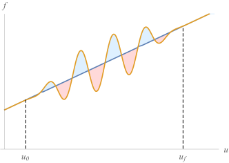
Figure 1: For an arbitrary function $f$, the operator $\Delta$ captures the total change in the function between the initial and final time. On the other hand, $\mathcal{R}$ captures the difference between the area under $f$ and its “trapezoidal” average $\overline{f}$.

2.3 Memory and balance equations

The balance equation (2.16) can be rearranged as

$$\frac{1}{4}\partial_{u}D^{A}D^{B}\left(C_{AB}+\frac{\lambda_{1}}{\lambda_{0}}\delta_{AB}\right)=\partial_{u}\mathcal{M}+\frac{1}{8}\dot{C}_{AB}\dot{C}^{AB}+(3+2\omega)\frac{1}{4\lambda_{0}^{2}}\left(\partial_{u}\lambda_{1}\right)^{2}\,.$$ (2.30)

Multiplying this with an arbitrary function $\varepsilon(x^{A})$ and integrating over the sphere and the time interval, we find

$$\frac{1}{4}\int_{S^{2}}\varepsilon D^{A}D^{B}\Delta C_{AB}=\Delta\mathcal{P}_{\varepsilon}+\mathcal{F}_{\varepsilon}\,,$$ (2.31)

where

$$\mathcal{P}_{\varepsilon}=\int_{S^{2}}\varepsilon\Big{(}\mathcal{M}-\frac{1}{4\lambda_{0}}\lambda_{1}\Big{)}$$ (2.32)

is the supermomentum charge with parameter $\varepsilon$ and its associated quadratic flux through the boundary is

$$\mathcal{F}_{\varepsilon}=\frac{1}{8}\int_{\Delta\mathcal{I}}\varepsilon\Big{(}\dot{C}_{AB}\dot{C}^{AB}+(3+2\omega)\frac{1}{4\lambda_{0}^{2}}\left(\partial_{u}\lambda_{1}\right)^{2}\Big{)}\,.$$ (2.33)

Throughout the paper, we use the shorthand notation

$$\int_{\Delta\mathcal{I}}\equiv\lim_{\rho\to\infty}\int_{u_{0}}^{u_{f}}du\int_{S^{2}},\qquad\int_{S^{2}}\equiv\int_{S^{2}}d^{2}x\sqrt{q}$$ (2.34)

We will justify in the next section that eq.(2.32) reduces to the standard expression for the supermomenta in the Einstein frame. Equation (2.31) determines the tensorial (shearing) part of the memory. However, the memory given by eq. (2.26), is characterized by the tensor $\Theta_{AB}$, which also contains a memory in its trace $\Theta$, called the breathing memory. Therefore, it is desirable to treat $\Delta\Theta$ in a similar manner, i.e. to write it in terms of a balance equation. To this end, we use the result (2.20) to arrive at

$$\frac{1}{8}\int_{S^{2}}\varepsilon D^{2}\Delta\Theta=\Delta Q_{\varepsilon}$$ (2.35)

where the quantity

$$Q_{\varepsilon}=-\frac{1}{4\lambda_{0}}\int_{S^{2}}\lambda_{1}D^{2}\varepsilon$$ (2.36)

can be thought of as a charge associated with the scalar field. We will justify this in the next section by showing that it is the Noether charge associated to the asymptotic symmetries of the dual formulation of the scalar field in BD theory. Subtracting eqs. (2.31) and (2.35), we find

$$\frac{1}{4}\int_{S^{2}}\varepsilon D^{A}D^{B}\Delta\Theta_{AB}=\Delta\mathcal{P}_{\varepsilon}+\mathcal{F}_{\varepsilon}+\Delta Q_{\varepsilon}\,.$$ (2.37)

In the next subsection, we show how the subleading displacement memory is fixed by another set of charges.

2.4 Subleading memory

The subleading part of the displacement memory is given by the second term in (2.29a). It is again sourced by tensorial and scalar modes. The former is related to the balance equations for the super Lorentz charges, as described in detail in Tahura:2020vsa ; Compere:2019gft . Let us focus here on the latter, i.e. the scalar contribution to the subleading memory. This part is characterized by

$$D^{2}\mathcal{R}\Theta =\int_{u_{0}}^{u_{f}}duD^{2}\big{(}\Theta-\overline{\Theta}\big{)}=-\frac{2}{\lambda_{0}}\int_{u_{0}}^{u_{f}}duD^{2}\big{(}\lambda_{1}-\overline{\lambda_{1}}\big{)}$$ (2.38)

Using the balance equation (2.14) for the scalar field, we can write the above expression smeared with a function $D^{2}\varepsilon$ as

$$-\frac{1}{8}\int_{S^{2}}D^{2}\varepsilon D^{2}\mathcal{R}\Theta =\Delta\mathcal{Q}_{\varepsilon}+\Delta u\,\overline{Q}_{D^{2}\varepsilon}$$ (2.39)

where the new charge is defined as

$$\mathcal{Q}_{\varepsilon}=-\frac{1}{2\lambda_{0}}\int_{S^{2}}\lambda_{2}D^{2}\varepsilon$$ (2.40)

We will show in the next section that this additional charge $\mathcal{Q}_{\varepsilon}$ is the Noether charge associated to overleading dual symmetries of the scalar field.

2.5 Inversion of the constraints

The constraints (2.35) and (2.39) can be inverted to find constraints over the memory effects appearing in (2.26). This can be done either by expansion in terms of spherical harmonics, or more formally through Green’s functions. Defining $Q_{\ell m}\equiv Q_{\varepsilon=Y_{\ell m}^{\ast}}$ and $\Delta\Theta=\sum_{\ell,m}\Delta\Theta^{{\ell m}}Y_{{\ell m}}$, we find from (2.35) that

$$\Delta\Theta^{{\ell m}}=-\frac{8}{\ell(\ell+1)}\Delta Q_{{\ell m}},\qquad\ell\geq 1$$ (2.41)

Therefore apart form the monopole of the breathing mode, all the multipole moments are given in terms of the fluxes of charges defined in (2.36). One can make the picture more coherent by defining a monopole charge

$$Q_{0}\equiv-\frac{1}{2\pi\lambda_{0}}\int_{S^{2}}\lambda_{1}$$ (2.42)

The above results can be written in a more compact form by inverting the Laplacian i.e. a Green function $G_{y}(x)=G(x,y)$ such that

$$D^{2}G(x,y)=\frac{1}{\sqrt{q}}\delta^{2}(x-y)-\frac{1}{4\pi}\,,\qquad x,y\in S^{2}.$$ (2.43)

The constant term is necessary so that both sides of the equation integrate to zero over the sphere. The Green function is explicitly given by

$$G(x,y)=\frac{1}{4\pi}\log\sin^{2}\frac{|x-y|}{2}+\text{const.}$$ (2.44)

where $|x-y|$ is the polar separation between the points $x^{A},y^{A}$ on the sphere. Using this in (2.35), and implementing the monopole charge (2.42), we find

$$\Delta\Theta(y) =8\Big{(}\Delta q+\Delta Q[\varepsilon(x)=G(x,y)]\Big{)}$$ (2.45)

where $y$ is a given point on the sphere and $x$ is a dummy variable integrated over in the charge integral. While the definition of the monopole charge $Q_{0}$ might look ad hoc at this stage, we will see in the next section that it is indeed a Noether charge with completely different origin from the higher multipole charges (2.36). Finally, we can invert the constraint (2.39) using a similar method, leading to

$$\mathcal{R}\Theta^{{\ell m}}=\frac{8}{\ell^{2}(\ell+1)^{2}}\Big{(}\Delta\mathcal{Q}_{{\ell m}}-\ell(\ell+1)\Delta u\,\overline{Q}_{{\ell m}}\Big{)},\qquad\ell\geq 1$$ (2.46)

It is not clear for us whether the monopole moment of $\mathcal{R}\Theta$ can be described using a flux equation or not.

2.6 Asymptotics in Einstein frame

By a redefinition of the fields as $\tilde{g}_{\mu\nu}=\frac{\lambda}{\lambda_{0}}{g}_{\mu\nu},\lambda=\exp(\phi/\Omega)$ with $\Omega=\sqrt{2\omega+3}$, the action of Brans-Dicke theory is transformed, up to surface terms, to that of GR with a minimally coupled scalar $\phi$

$$S=\lambda_{0}\int d^{4}x\sqrt{-\tilde{g}}\Big{[}\tilde{R}-\frac{1}{2}\tilde{g}^{{\mu\nu}}\partial_{\mu}\phi\partial_{\nu}\phi\Big{]}$$ (2.47)

The metric $\tilde{g}_{\mu\nu}$ as defined above satisfies the gauge conditions (2.4) except the determinant condition, since $\sqrt{\det\tilde{g}_{AB}}=\frac{\lambda}{\lambda_{0}}\sqrt{\det{g}_{AB}}=\frac{\lambda}{\lambda_{0}}r^{2}\sqrt{q}$. This is because the radial coordinate is the areal distance with respect to ${g}_{\mu\nu}$ and not $\tilde{g}_{\mu\nu}$. It is still possible to perform a simple redefinition of the radial coordinate as

$$\rho =r\sqrt{\frac{\lambda}{\lambda_{0}}}=r+\frac{\lambda_{1}}{2\lambda_{0}}+\mathcal{O}(1/r)$$ (2.48)

so that the metric $\tilde{g}_{\mu\nu}(u,\rho,x^{A})$ is in Bondi gauge. This implies that the conformal map between the two frames should be accompanied by a coordinate transformation. Explicitly, denoting $\tilde{x}^{\mu}=(u,\rho,x^{A})$, $x^{\mu}=(u,r,x^{A})$, then

$$\tilde{g}_{\mu\nu}(\tilde{x})=\frac{\lambda(x)}{\lambda_{0}}\frac{\partial x^{\alpha}}{\partial\tilde{x}^{\mu}}\frac{\partial x^{\beta}}{\partial\tilde{x}^{\nu}}{g}_{\alpha\beta}(x),\qquad\lambda(x)=\lambda_{0}\exp\Big{(}\frac{\phi(\tilde{x})-\phi_{0}}{\Omega}\Big{)}$$ (2.49)

Using (2.49) and the results of the previous section, one can obtain the asymptotic behavior of the fields in the Einstein frame. In particular, assuming an asymptotic expansion for the scalar as $\phi=\sum_{n=0}^{\infty}\phi_{n}(u,x^{A})\rho^{-n}$, we can find the relation between the scalars in the two frames. Note that

$$e^{(\phi-\phi_{0})/\Omega} =1+\frac{1}{\rho\Omega}\phi_{1}(u,x^{A})+\frac{1}{\rho^{2}\Omega}\big{(}\phi_{2}+\frac{\phi_{1}^{2}}{2\Omega}\big{)}+\cdots$$ (2.50)

However, after replacing $\rho$ with $r$ perturbatively using (2.48) we find that

$$\frac{\lambda_{1}}{\lambda_{0}}=\frac{\phi_{1}}{\Omega},\qquad\frac{\lambda_{2}}{\lambda_{0}}=\frac{\phi_{2}}{\Omega}$$ (2.51)

and a balance equation holds for the subleading component of the scalar

$$\dot{\phi}_{2} =-\frac{1}{2}D^{2}\phi_{1}$$ (2.52)

On the other hand, the metric being in Bondi gauge takes the form

$$ds^{2} =e^{2b}\big{(}{V}du^{2}-2du\,d\rho\big{)}+\rho^{2}h_{AB}(dx^{A}-V^{A}du)(dx^{B}-V^{B}du)$$ (2.53)

$$h_{AB} ={\tilde{q}}_{AB}+{\rho}^{-1}{\tilde{C}}_{AB}+\mathcal{O}(\rho^{-2})\,, b=\mathring{b}\,\rho^{-2}+\mathcal{O}(\rho^{-3})$$

$${V}^{A} =\mathring{V}^{A}\rho^{-2}+\mathcal{O}(\rho^{-3})\,, {V}=\mathring{V}-2M\rho^{-1}+\mathcal{O}\left({\rho}^{-2}\right)\,,$$ (2.54)

where the relationship between these asymptotic coefficients and those of Jordan frame (2.12) is obtained as

$$\tilde{q}_{AB} =q_{AB}\,\qquad\tilde{C}_{AB}=C_{AB}\,,\qquad\mathring{b}=\mathring{\beta}-\frac{1}{8}\phi_{1}^{2}\,,\qquad\mathring{V}^{A}=\mathring{U}^{A}\,,\qquad\mathring{V}=-\frac{R[q]}{2}$$ (2.55)

Note that there is no radial dependence in the above quantities, e.g. $\tilde{C}_{AB}(u,x^{A})=C_{AB}(u,x^{A})$. Therefore, in the following, we will always replace $\tilde{q}_{AB},\tilde{C}_{AB}$ in favor of the ones without tilde. Finally, the relationship between the mass aspects in the two frames is

$$M=m-\frac{\phi_{1}\dot{\phi}_{1}}{4\Omega^{2}}+\frac{1}{2\Omega}\dot{\phi}_{2}=\mathcal{M}-\frac{1}{4\lambda_{0}}D^{2}\lambda_{1}\,.$$ (2.56)

Given that in the Einstein frame, the theory is Einstein GR plus a minimally coupled scalar, it is well known that the supermomenta take the form $\mathcal{P}_{\varepsilon}=\oint\varepsilon M$. Using (2.56), we see that this coincides with (2.32) in the Jordan frame.

3 The interplay between memory and symmetry

In previous section, it was shown that the description of the breathing memory motivates two sets of charges given in eqs. (2.36),(2.40). Given that BD theory has no additional local symmetry other than the diffeomorphisms, it is natural to ask which symmetries these charges correspond to? In Campiglia:2018see , this question was partly addressed in a non-gravitational context, where it was shown that the leading charges (2.36) correspond to the asymptotic symmetries of a dual formulation of the scalar in terms of two-form gauge fields. Here we extend their results to the gravitational context. Moreover, we show that the subleading charges (2.40) are also Noether charges associated to a set of “overleading” symmetries of the gauge field.

3.1 Dual formulation of the scalar

Introduction.

Let us consider a theory of two form field $B=\frac{1}{2}B_{\mu\nu}dx^{\mu}dx^{\nu}$ with the Lagrangian $\mathcal{L}=-\frac{1}{2}{H}\wedge*{H}$, where $H=dB$ is the corresponding field strength. The field equation and the Bianchi identity read

$$d\ast H=0\,,\qquad dH=0\,,$$ (3.1)

which imply respectively that

$$H=\ast d\phi\,,\qquad\Box\phi=d\ast d\phi=0\,,$$ (3.2)

for some scalar field $\phi$. Replacing the first equality back into the Lagrangian, we find that $\mathcal{L}=-\frac{1}{2}d\phi\wedge*d\phi$, which coincides with that of a free scalar field. In this sense, the two form theory is dual to a free scalar theory. Note that the role of field equation and Bianchi identity is exchanged when going to the dual picture. This construction is independent of the metric of spacetime and therefore can be used in a gravitational theory as well. The only consistency requirement imposed by the Bianchi identity is that the field equation for the scalar field has no source term. This is the case for Brans-Dicke theory even in the presence of electromagnetic matter fields. Therefore, in this section we propose to consider the following dual action instead of (2.47):

$$S=\int d^{4}\tilde{x}\sqrt{-{\tilde{g}}}\left[\tilde{R}-\frac{1}{12}H_{{\mu\nu}\alpha}H^{{\mu\nu}\alpha}\right]\,,$$ (3.3)

where the tilde reminds that we are working in the Einstein frame, where the coordinates are $\tilde{x}^{\mu}=(u,\rho,x^{A})$ and the metric is given by (2.53). For simplicity, we do not put tilde over the gauge fields, which should not lead to any confusion.

3.2 Asymptotic behavior of the gauge field

We simplify the analysis by imposing the following gauge conditions on the gauge field

$$B_{u\rho}=B_{uA}=0\,,\qquad D^{A}B_{\rho A}=0\,.$$ (3.4)

The latter condition is primarily imposed on an initial hypersurface $u=const$. However, the field equations extend it to allover the spacetime. As in the previous section, we use the leading metric $q_{AB}$ to raise and lower indices on the sphere, and to define the connection $D_{A}$. Now consider the following asymptotic expansion for the remaining components

$$\begin{split}{B}_{\rho A}&=\sum_{n=-\infty}^{N-1}\rho^{n}B_{\rho A}^{(n)}(u,x^{A}),\qquad{B}_{AB}=\sum_{n=-\infty}^{N}\rho^{n}B_{AB}^{(n)}(u,x^{A})\end{split}$$ (3.5)

where $N$ is a positive integer that we will come back to soon. Note that contrary to the expansion of the scalar field $\phi$, here positive $n$ refers to the coefficient of a positive power of $\rho$. This asymmetric notation simplifies the results in the following. To find the asymptotic behavior of the gauge field, we need to solve eq.(3.2) for the gauge field $B$. Note that

while the right hand side of (3.2) is given by

$$(\tilde{\ast}d\phi)_{u\rho A} =-\epsilon_{AB}(e^{2b}h^{BC}\partial_{C}\phi-\rho^{2}U^{B}\partial_{\rho}\phi)=-\epsilon_{A}^{\;\;\;B}\partial_{B}\frac{\phi_{1}}{\rho}+\mathcal{O}(\rho^{-2})$$ (3.6a)

$$(\tilde{\ast}d\phi)_{uAB} =\rho^{2}\epsilon_{AB}\big{(}\dot{\phi}+V\partial_{\rho}\phi+V^{A}\partial_{A}\phi\big{)}=\rho\,\epsilon_{AB}\,\dot{\phi}_{1}+\mathcal{O}(1)$$ (3.6b)

$$(\tilde{\ast}d\phi)_{\rho AB} =-\rho^{2}\epsilon_{AB}\partial_{\rho}\phi=\epsilon_{AB}(\phi_{1}+2\frac{\phi_{2}}{\rho})+\mathcal{O}(1/\rho^{2})$$ (3.6c)

To compare the two form theory and the scalar theory more easily, we note that the gauge condition $D^{A}B_{\rho A}=0$ allows to write $B_{\rho A}$ in terms of one scalar field. On the other hand $B_{AB}$ being a two form on the sphere is necessarily proportional to the Levi-Civita tensor, so we can write

$$B_{\rho A}=\epsilon_{A}^{\;\;\;B}\partial_{B}\partial_{\rho}\sigma,\qquad B_{AB}=\epsilon_{AB}\psi$$ (3.7)

Using (3.7) in (3.6c), we get

$${H}_{\rho AB}=\partial_{\rho}B_{AB}+2\partial_{[A}B_{B]\rho}=\epsilon_{AB}\partial_{\rho}\left(\psi+D^{2}\sigma\right)$$ (3.8)

where we have used the fact that in two dimensions, antisymmetrization of two indices can be trade off with the Levi-Civita tensor

$$2u_{[A}v_{B]}=(\delta_{A}^{\;\;C}\delta_{B}^{\;\;D}-\delta_{B}^{\;\;C}\delta_{A}^{\;\;D})u_{C}v_{D}=\epsilon_{AB}\epsilon^{CD}u_{C}v_{D}$$

Comparing (3.8) and the third equation in (3.6), we find

$$\partial_{\rho}\big{(}\psi+D^{2}\sigma\big{)}+\rho^{2}\partial_{\rho}\phi =0\,,$$ (3.9)

Using the asymptotic expansion with an asymptotic expansion

$$\sigma =\sum_{n=-\infty}^{N}\rho^{n}\sigma_{n}+\bar{\sigma}\log\rho,\qquad\psi=\sum_{n=-\infty}^{N}\rho^{n}\psi_{n}\,.$$ (3.10)

we find

$$\psi_{1} =\phi_{1}-D^{2}\sigma_{1}\,,$$ (3.11a)

$$\psi_{n} =-D^{2}\sigma_{n}\,,\qquad n\geq 2\,,$$ (3.11b)

Also equating the first and second equations in (3.2) and (3.6), we find that

$$\bar{\sigma}=-\int du\phi_{1}\,,\qquad\text{and}\qquad\partial_{u}\sigma_{n}=0\,,\quad n\geq 0$$ (3.12)

This suffices for our analysis of symmetries and charges in the next section.

3.3 Phase space structure

The asymptotic solutions discussed in the previous section can be given a canonical structure. This is most conveniently obtained by using the covariant phase space approach Ashtekar:1981bq ; Wald:1999wa . The covariant phase space is defined as the collection of asymptotic solutions accompanied by a symplectic structure. Focusing on the two form field, we find through a standard procedure that the symplectic current as a spacetime three form is given by

$$\omega_{B}=\delta\ast H\wedge\delta{B}=\delta d\phi\wedge\delta{B}$$ (3.13)

where the $\wedge$ denotes antisymmetrization of the phase space variations, combined with the spacetime wedge product. The symplectic structure of the radiative phase space is obtained by integrating the symplectic current over a worldtube at large constant radius between the initial time $u_{0}$ when the system is nonradiative to $u_{f}$ at which the system again goes back to a nonradiative configuration. The relevant component is $\omega^{B}_{uAB}=\frac{1}{2}\,\delta\dot{\phi}\wedge\delta B_{AB}$. Using (3.7) and taking the integral, we find

$$\Omega_{B} =\int_{\Delta\mathcal{I}}\delta\dot{\phi}\wedge\delta\psi$$ (3.14)

With the general asymptotic behavior for $B_{AB}$ implied by (3.10), the symplectic structure $\Omega_{B}$ diverges as $\rho^{N-1}$. The divergence can be removed by imposing the boundary condition $B_{AB}=\rho B^{(1)}_{AB}+\mathcal{O}(1)$, as done in Campiglia:2018see , leading to the following symplectic structure of the radiative phase space

$$\Omega_{(1)} =\int_{\Delta\mathcal{I}}\delta\dot{\phi}_{1}\wedge\delta\psi_{1}=\int_{\Delta\mathcal{I}}\delta\dot{\phi}_{1}\wedge\delta(\phi_{1}-D^{2}\sigma_{1})\,.$$ (3.15)

A more heuristic approach, which we will follow in this work is to define a the symplectic structure as the finite part of the bare symplectic form (3.14). The regularized symplectic structure is found by making an asymptotic expansion of all fields and keeping the $\rho$ independent piece of the bare symplectic structure (3.14). We then find

$$\Omega_{\text{reg}}=\sum_{n=1}^{N}\Omega_{(n)},\qquad\Omega_{(n)}=\int_{\Delta\mathcal{I}}\,\delta\dot{\phi}_{n}\wedge\delta\psi_{n}$$ (3.16)

It turns out that this approach is more informative than the other one, as it allows to define a tower of overleading symmetries, their charges and balance equations which in turn allow to discuss all memory effects coherently. Overleading symmetries have shown up in different fashions in the literature, including multipole symmetries in gauge theory and gravity Seraj:2016jxi ; Seraj:2017rzw ; Compere:2017wrj ; Kutluk:2019ghr , as well as those inspired by subleading soft theorems Campiglia:2016efb ; Campiglia:2018dyi ; Laddha:2017vfh ; Conde:2016csj and adiabatic modes Mirbabayi:2016xvc ; Hamada:2018vrw .

Note that the symplectic structure of the scalar theory and its dual two form theory are not the same. The symplectic structure of the scalar field is given by $\Omega_{\phi}=\int_{\Delta\mathcal{I}}\delta\dot{\phi}_{1}\wedge\delta\phi_{1}$. Comparing this with (3.14), we see that they differ by

$$\Omega_{\text{reg}}-\Omega_{\phi} =-\sum_{n=1}^{N}\int_{\Delta\mathcal{I}}\delta\dot{\phi}_{n}\wedge\delta D^{2}\sigma_{n}=-\sum_{n=1}^{N}\int_{S^{2}}\delta\Delta\phi_{n}\wedge\delta D^{2}\sigma_{n}$$ (3.17)

where we used the fact that $\sigma_{n}$ is time independent for $n\geq 1$. The full symplectic structure contains additional non-radiative edge modes that lead to nontrivial symmetries and charges, which in turn explain the memory effects.

Adding the standard contribution from the GR sector Ashtekar:1981bq , the full symplectic structure of the theory is given by

$$\Omega =\int_{\Delta\mathcal{I}}\left(\delta\dot{C}^{AB}\wedge\delta C_{AB}+\delta\dot{\psi}_{1}\wedge\delta\psi_{1}\right)-\sum_{n=2}^{N}\int_{S^{2}}\delta\Delta\phi_{n}\wedge\delta D^{2}\sigma_{n}$$ (3.18a)

$$=\int_{\Delta\mathcal{I}}\left(\delta\dot{C}^{AB}\wedge\delta C_{AB}+\delta\dot{\phi}_{1}\wedge\delta\phi_{1}\right)-\sum_{n=1}^{N}\int_{S^{2}}\delta\Delta\phi_{n}\wedge\delta D^{2}\sigma_{n}$$ (3.18b)

In the last line, The first integral denotes the radiative phase space of gravitational degrees of freedom, while the second integral represents the phase space of edge modes whose conjugate momenta are related to the gravitational memories as we will discuss.

3.4 Symmetries and balance equations

The theory is (3.3) is invariant under transformations

$$B\to B+\alpha,\qquad d\alpha=0$$ (3.19)

Moreover, $\alpha$ should have the same asymptotic behavior as in eq.(3.5) and should preserve the temporal gauge we have imposed. The solution is given by $\alpha=-d\beta$ with

$$\beta=\beta_{A}dx^{A}\,,\qquad\beta_{A}=\epsilon_{A}^{\;\;\;B}\partial_{B}\,\mu(\rho,x^{A})\,.$$ (3.20)

In terms of the fields defined in (3.7), this corresponds to the shift

$$\sigma\to\sigma-\mu(\rho,x^{A})\,,\qquad\psi\to\psi+D^{2}\mu(\rho,x^{A})$$ (3.21)

In other words, by expanding the symmetry parameter as $\mu=\sum_{n=-\infty}^{N}\rho^{n}\varepsilon_{n}(x^{A})$, we find a tower of symmetry transformations

$$\sigma_{n}\to\sigma_{n}-\varepsilon_{n}(x^{A})\,\qquad\psi_{n}\to\psi_{n}+D^{2}\varepsilon_{n}(x^{A})\,.$$ (3.22)

Whether these are redundant pure gauge transformations or physical asymptotic symmetries is determined by the symplectic structure of the theory. If the contraction of the symplectic structure with a variation $\delta_{\varepsilon}$ is zero, then this variation is a degeneracy of the symplectic form and hence quotiented out in the physical phase space. However, if $\Omega(\delta,\delta_{\varepsilon})\neq 0$ for some $\delta$ tangent to the phase space, then $\varepsilon$ represents an asymptotic symmetry and is associated with a nontrivial charge on the physical phase space. Noting (3.18a), we see that $\varepsilon_{n}$ is nontrivial for $n\geq 1$.

Tower of Charges and fluxes.

By contracting the symplectic structure with a symmetry transformation, we can define a flux associated to that symmetry, i.e. $\delta\mathcal{F}_{\varepsilon}=\Omega(\delta,\delta_{\varepsilon})$. Using (3.18a), and considering the symmetry transformation (3.22),

$$\mathcal{F}_{n}[\varepsilon]=\int_{S^{2}}\Delta\phi_{n}D^{2}\varepsilon\,,\qquad n\geq 1$$ (3.23)

The flux can be written as the change in a Noether charge associated to the symmetry. In other words, we have the flux-balance equation $\mathcal{F}_{n}[\varepsilon]=-\Delta Q_{n}[\varepsilon]$ where

$$Q_{n}[\varepsilon]=-\int_{S^{2}}\phi_{n}D^{2}\varepsilon\,,\qquad n\geq 1$$ (3.24)

In summary, we have a tower of charges labeled by $n$ and at each level, we have infinitely many charges parameterized by an arbitrary function $\varepsilon_{n}(x^{A})$ on the sphere. Also it is important to note that the charges $Q_{1}[\varepsilon]$ does not contain the monopole charge as the monopole is in the kernel of the Laplacian appearing in the definition of the charge (3.24). However, looking at the second term in the symplectic structure (3.18a), we see that a constant shift $\phi\to\phi+c$ is an independent symmetry of the symplectic form and leads to an additional charge

$$q=-\int_{S^{2}}\phi_{1}$$ (3.25)

This charge corresponds to the shift symmetry of the original scalar theory. Therefore, the full symmetry algebra is the union of the symmetries of the dual frames. This is similar to electric and magnetic charges in Maxwell theory; while the (asymptotic) electric charges appear naturally as Noether charges corresponding to the large gauge symmetries in the standard description of the theory, magnetic charges play the same role in the dual description of the theory. Remarkably, both set of charges are physical observables in either of the descriptions and are given by local expressions of the fields.

Let us focus on the first sets of charges $q,\,Q_{1}[\varepsilon],\,Q_{2}[\varepsilon]$. Note that using eq.(2.51), we get

$$q=4\Omega Q_{0}\,,\qquad Q_{1}[\varepsilon]=4\Omega Q_{\varepsilon}\,,\qquad Q_{2}[\varepsilon]=2\Omega\mathcal{Q}_{\varepsilon}$$ (3.26)

Therefore, up to trivial normalization constants, these are the charges whose balance equations determine the breathing memory effects in Brans-Dicke theory, as was shown in the previous section, eqs. (2.42), (2.36) and (2.40).

3.5 Memory as vacuum transition

There is a second aspect of the relationship between memory effects and BMS symmetries. Suppose that the spacetime is non-radiative before and after a burst of gravitational wave lasting between the time interval $(u_{0},u_{f})$. From the perspective of the radiative phase space given by the symplectic structure (3.15), the system is in vacuum state before $u_{0}$ and after $u_{f}$. However, these vacua are not identical precisely due to the memory effect. Therefore, instead of a single vacuum, the radiative phase space possesses a “space of vacua”. The space of vacua is a subspace of the covariant phase space on which the pull back of the symplectic form vanishes. From (3.15), we see that this subspace is given by time independent functions $\psi_{1}(x^{A})$. The gravitational memory effect causes a transition between an initial vacuum $\psi_{1}^{(0)}$ and a final one $\psi_{1}^{(f)}$. Now we show that the vacuum transition can be modeled by a symmetry transformation. To see this, note that by construction, the charges introduced in the previous section satisfy

$$\big{\{}Q_{1}[\varepsilon],\psi_{1}\big{\}} =D^{2}\varepsilon\,,\qquad \big{\{}Q_{1}[\varepsilon],\sigma_{1}\big{\}} =-\varepsilon\,$$ (3.27a)

$$\big{\{}q,\psi_{1}\big{\}} =1\,, \big{\{}q,\sigma_{1}\big{\}} =0$$ (3.27b)

Therefore we can find a constant $c$ and a function $\varepsilon$ such that

$$\psi_{1}^{(f)} =\psi_{1}^{(0)}+\big{\{}c\,q+Q_{1}[\varepsilon],\psi_{1}^{(0)}\big{\}}$$ (3.28)

Also note that according to (3.11a), $\phi_{1}=\psi_{1}+D^{2}\sigma_{1}$ and therefore

$$\big{\{}Q_{1}[\varepsilon],\phi_{1}\big{\}} =0$$ (3.29)

Therefore $\phi_{1}$ is gauge invariant which explains why there is no gauge symmetry in the scalar field formulation.

4 Discussion

In this work, we discussed gravitational memory effects in Brans-Dicke theory. This can be considered as a means to test general relativity, as a nonvanishing breathing memory signals deviation from general relativity Du:2016hww . It is desirable to study various permanent effects due to the scalar mode and to compute the breathing memory for particular dynamical sources, for example how scalarization processes are encoded in the memory. The memory effects in more realistic scalar-tensor theories are even more interesting, as the scalar memory can be significantly enhanced as a result of the screening mechanism Koyama:2020vfc .

At a theoretical level, we showed that the breathing memory effect in BD theory can be explained through a symmetry principle by taking into account “dual symmetries”, i.e. the asymptotic symmetries of a dual formulation of the scalar field in terms of two-form gauge fields. Our construction relied on the fact that the scalar field is massless and free. This is not the case in the presence of generic matter fields, or in more general scalar-tensor theories. This suggests that there exists a more general way to define dual symmetries, e.g. through an asymptotic notion of the duality Freidel:2018fsk .

Our construction revealed a tower of asymptotic charges given in eq. (3.24). At $n=2$, a remaining issue is that the subleading memory can contain monopole mode, which is not captured by the charges that we obtained. For more subleading charges $n>2$, it is important to see if they are related to new low energy effects. The subsubleading soft dilaton factorization of DiVecchia:2015jaq , valid at tree level, suggests that this is the case.

We obtained the tower of charges through a regularized symplectic structure obtained through a finite part prescription. It is desirable to find this result in a more systematic fashion, e.g. by adding suitable counterterms in the action.

Acknowledgments

I thank Erfan Esmaeili and David Nichols for useful discussions. The author is funded by the European Union’s Horizon 2020 research and innovation program under the Marie Sklodowska-Curie grant agreement No 801505.

Appendix A Null congruences in Bondi gauge

To compare the asymptotic behavior in BD and GR, it would be useful to study the behavior of the congruence of future directed outgoing and ingoing null dyad

$$\ell=\partial_{r}\,,\qquad n=n_{\mu}dx^{\mu}=e^{-2\beta}(\partial_{u}+\frac{U}{2}\partial_{r}+U^{A}\partial_{A})\,,$$ (A.1)

The latter can be written as a dual 1-form as $n=\frac{U}{2}du-dr$ from which it is obvious that $\ell\cdot n=-1$. The ingoing null vector takes the asymptotic form $n=\partial_{u}+\frac{\mathring{U}}{2}\partial_{r}+\mathcal{O}(1/r)$, so that in Jordan frame

$$n=\partial_{u}-\frac{1}{2}(1+\frac{\dot{\lambda}_{1}}{\lambda_{0}})\partial_{r}+\mathcal{O}(1/r)$$ (A.2)

Remind that a null congruence with tangent vector $k$ can be described in terms of expansion, shear and twist

$$\nabla_{A}k_{B}=\frac{1}{2}\theta g_{AB}+\sigma_{AB}+\omega_{AB}$$ (A.3)

with

$$\theta=g^{AB}\nabla_{A}k_{B},\qquad\sigma_{AB}=\nabla_{(A}k_{B)}-\frac{1}{2}\theta g_{AB},\qquad\omega_{AB}=\nabla_{[A}k_{B]}$$ (A.4)

Both the congruences of (A.1) are twist-free. For the outgoing congruence of $\ell$, the expansion and shear coincide asymptotically with that of GR

$$\nabla_{(A}\ell_{B)}=rq_{AB}+\frac{1}{2}C_{AB}+\mathcal{O}(1/r)$$ (A.5)

while for the ingoing vector $n$, there is a dynamical mode in its expansion

$$\nabla_{(A}n_{B)}=-\frac{r}{2}\Big{(}\dot{C}_{AB}+q_{AB}\mathring{U}\Big{)}+\mathcal{O}(1)$$ (A.6)

since $\mathring{U}=-(\frac{1}{2}R[q]+\frac{\lambda_{1}}{\lambda_{0}})$. From the above null vectors, we can construct unit timelike and spacelike vectors

$$\hat{e}_{0}=n+\ell/2\,,\qquad\hat{e}_{r}=n-\ell/2$$ (A.7)

reproducing (2.18). An interesting property of Bondi gauge in GR is that the Bondi frame asymptotically reduces to an inertial frame, as can be seen by setting $\lambda=0$ in (2.18). However, this is not anymore the case in BD theory. A test mass at rest in the inertial frame has four-velocity

$$v^{\mu}\partial_{\mu}=\hat{e}_{0}=\partial_{u}-\frac{1}{2\lambda_{0}}\dot{\lambda}_{1}{\partial}_{r}.$$

Therefore, this worldline is described in the Bondi coordinates as radially oscillating. However, this coordinate effect disappears when studying geodesic deviation. It is also possible to modify the Bondi gauge such that the coordinate and inertial frames coincide asymptotically. One has to replace (2.11) by the modified determinant condition

$$\det(g_{AB})=r^{4}(\frac{\lambda}{\lambda_{0}})^{2}\det(q_{AB})$$ (A.8)

This implies that the Bondi tensor $C_{AB}$ will have a trace (expansion) part as well. Imposing (A.8) might look strange, but it is natural from the perspective that the transverse field $C_{AB}$ contains all the propagating degrees of freedom, consisting of the shearing $+,\times$ polarization modes, as well the scalar breathing mode. It is also equivalent to imposing that $r$ is the areal distance but with respect to the metric in the Einstein frame. This approach was followed in Hou:2020tnd .

References

- (1) Y. B. Zel’dovich and A. G. Polnarev, Radiation of gravitational waves by a cluster of superdense stars, Sov. Astron. 18 (1974) 17.
- (2) D. Christodoulou, Nonlinear nature of gravitation and gravitational wave experiments, Phys. Rev. Lett. 67 (1991) 1486–1489.
- (3) L. Blanchet and T. Damour, Hereditary effects in gravitational radiation, Phys. Rev. D 46 (1992) 4304–4319.
- (4) H. Bondi, M. G. J. van der Burg and A. W. K. Metzner, Gravitational waves in general relativity. 7. Waves from axisymmetric isolated systems, Proc. Roy. Soc. Lond. A 269 (1962) 21–52.
- (5) R. K. Sachs, Gravitational waves in general relativity. 8. Waves in asymptotically flat space-times, Proc. Roy. Soc. Lond. A 270 (1962) 103–126.
- (6) A. Strominger and A. Zhiboedov, Gravitational Memory, BMS Supertranslations and Soft Theorems, JHEP 01 (2016) 086 [1411.5745].
- (7) A. Strominger, Lectures on the Infrared Structure of Gravity and Gauge Theory, 1703.05448.
- (8) G. Barnich and C. Troessaert, Aspects of the BMS/CFT correspondence, JHEP 05 (2010) 062 [1001.1541].
- (9) M. Campiglia and A. Laddha, Asymptotic symmetries and subleading soft graviton theorem, Phys. Rev. D 90 (2014), no. 12 124028 [1408.2228].
- (10) M. Campiglia and A. Laddha, New symmetries for the Gravitational S-matrix, JHEP 04 (2015) 076 [1502.02318].
- (11) S. Pasterski, A. Strominger and A. Zhiboedov, New Gravitational Memories, JHEP 12 (2016) 053 [1502.06120].
- (12) D. A. Nichols, Center-of-mass angular momentum and memory effect in asymptotically flat spacetimes, Phys. Rev. D 98 (2018), no. 6 064032 [1807.08767].
- (13) L. Bieri and D. Garfinkle, An electromagnetic analogue of gravitational wave memory, Class. Quant. Grav. 30 (2013) 195009 [1307.5098].
- (14) S. Pasterski, Asymptotic Symmetries and Electromagnetic Memory, JHEP 09 (2017) 154 [1505.00716].
- (15) M. Campiglia, L. Coito and S. Mizera, Can scalars have asymptotic symmetries?, Phys. Rev. D 97 (2018), no. 4 046002 [1703.07885].
- (16) M. Campiglia, L. Freidel, F. Hopfmueller and R. M. Soni, Scalar Asymptotic Charges and Dual Large Gauge Transformations, JHEP 04 (2019) 003 [1810.04213].
- (17) D. Francia and C. Heissenberg, Two-Form Asymptotic Symmetries and Scalar Soft Theorems, Phys. Rev. D 98 (2018), no. 10 105003 [1810.05634].
- (18) H. Afshar, E. Esmaeili and M. M. Sheikh-Jabbari, Asymptotic Symmetries in -Form Theories, JHEP 05 (2018) 042 [1801.07752].
- (19) E. Esmaeili, -form gauge fields: charges and memories, other thesis, 10, 2020.
- (20) V. Hosseinzadeh, A. Seraj and M. M. Sheikh-Jabbari, Soft Charges and Electric-Magnetic Duality, JHEP 08 (2018) 102 [1806.01901].
- (21) L. Freidel and D. Pranzetti, Electromagnetic duality and central charge, Phys. Rev. D 98 (2018), no. 11 116008 [1806.03161].
- (22) M. Henneaux and C. Troessaert, A note on electric-magnetic duality and soft charges, JHEP 06 (2020) 081 [2004.05668].
- (23) H. Godazgar, M. Godazgar and C. N. Pope, New dual gravitational charges, Phys. Rev. D 99 (2019), no. 2 024013 [1812.01641].
- (24) U. Kol and M. Porrati, Properties of Dual Supertranslation Charges in Asymptotically Flat Spacetimes, Phys. Rev. D 100 (2019), no. 4 046019 [1907.00990].
- (25) H. Godazgar, M. Godazgar and C. N. Pope, Dual gravitational charges and soft theorems, JHEP 10 (2019) 123 [1908.01164].
- (26) H. Godazgar, M. Godazgar and M. J. Perry, Hamiltonian derivation of dual gravitational charges, JHEP 20 (2020) 084 [2007.07144].
- (27) R. Oliveri and S. Speziale, A note on dual gravitational charges, JHEP 12 (2020) 079 [2010.01111].
- (28) R. N. Lang, Compact binary systems in scalar-tensor gravity. II. Tensor gravitational waves to second post-Newtonian order, Phys. Rev. D 89 (2014), no. 8 084014 [1310.3320].
- (29) R. N. Lang, Compact binary systems in scalar-tensor gravity. III. Scalar waves and energy flux, Phys. Rev. D 91 (2015), no. 8 084027 [1411.3073].
- (30) S. M. Du and A. Nishizawa, Gravitational Wave Memory: A New Approach to Study Modified Gravity, Phys. Rev. D 94 (2016), no. 10 104063 [1609.09825].
- (31) K. Koyama, Testing Brans-Dicke Gravity with Screening by Scalar Gravitational Wave Memory, Phys. Rev. D 102 (2020), no. 2 021502 [2006.15914].
- (32) S. Tahura, D. A. Nichols, A. Saffer, L. C. Stein and K. Yagi, Brans-Dicke theory in Bondi-Sachs form: Asymptotically flat solutions, asymptotic symmetries and gravitational-wave memory effects, 2007.13799.
- (33) S. Hou and Z.-H. Zhu, ”Conserved charges” of the Bondi-Metzner-Sachs algebra in the Brans-Dicke theory, Chin. Phys. C 45 (2021), no. 2 023122 [2008.05154].
- (34) S. Hou and Z.-H. Zhu, Gravitational memory effects and Bondi-Metzner-Sachs symmetries in scalar-tensor theories, JHEP 01 (2021) 083 [2005.01310].
- (35) D. A. Nichols, Spin memory effect for compact binaries in the post-Newtonian approximation, Phys. Rev. D 95 (2017), no. 8 084048 [1702.03300].
- (36) P. Di Vecchia, R. Marotta, M. Mojaza and J. Nohle, New soft theorems for the gravity dilaton and the Nambu-Goldstone dilaton at subsubleading order, Phys. Rev. D 93 (2016), no. 8 085015 [1512.03316].
- (37) A. Ashtekar, Geometry and Physics of Null Infinity, 1409.1800.
- (38) G. Compère, A. Fiorucci and R. Ruzziconi, Superboost transitions, refraction memory and super-Lorentz charge algebra, JHEP 11 (2018) 200 [1810.00377]. [Erratum: JHEP 04, 172 (2020)].
- (39) G. Compère, R. Oliveri and A. Seraj, The Poincaré and BMS flux-balance laws with application to binary systems, JHEP 10 (2020) 116 [1912.03164].
- (40) A. Ashtekar and M. Streubel, Symplectic Geometry of Radiative Modes and Conserved Quantities at Null Infinity, Proc. Roy. Soc. Lond. A 376 (1981) 585–607.
- (41) R. M. Wald and A. Zoupas, A General definition of ’conserved quantities’ in general relativity and other theories of gravity, Phys. Rev. D 61 (2000) 084027 [gr-qc/9911095].
- (42) A. Seraj, Multipole charge conservation and implications on electromagnetic radiation, JHEP 06 (2017) 080 [1610.02870].
- (43) A. Seraj and D. Van den Bleeken, Strolling along gauge theory vacua, JHEP 08 (2017) 127 [1707.00006].
- (44) G. Compère, R. Oliveri and A. Seraj, Gravitational multipole moments from Noether charges, JHEP 05 (2018) 054 [1711.08806].
- (45) E. c. Kutluk, A. Seraj and D. Van Den Bleeken, Strolling along gravitational vacua, JHEP 01 (2020) 184 [1904.12869].
- (46) M. Campiglia and A. Laddha, Sub-subleading soft gravitons and large diffeomorphisms, JHEP 01 (2017) 036 [1608.00685].
- (47) M. Campiglia and A. Laddha, Asymptotic charges in massless QED revisited: A view from Spatial Infinity, JHEP 05 (2019) 207 [1810.04619].
- (48) A. Laddha and P. Mitra, Asymptotic Symmetries and Subleading Soft Photon Theorem in Effective Field Theories, JHEP 05 (2018) 132 [1709.03850].
- (49) E. Conde and P. Mao, Remarks on asymptotic symmetries and the subleading soft photon theorem, Phys. Rev. D 95 (2017), no. 2 021701 [1605.09731].
- (50) M. Mirbabayi and M. Simonović, Weinberg Soft Theorems from Weinberg Adiabatic Modes, 1602.05196.
- (51) Y. Hamada and G. Shiu, Infinite Set of Soft Theorems in Gauge-Gravity Theories as Ward-Takahashi Identities, Phys. Rev. Lett. 120 (2018), no. 20 201601 [1801.05528].