Multi-field, multi-frequency bosonic stars and a stabilization mechanism

Abstract

Scalar bosonic stars (BSs) stand out as a multi-purpose model of exotic compact objects. We enlarge the landscape of such (asymptotically flat, stationary, everywhere regular) objects by considering multiple fields (possibly) with different frequencies. This allows for new morphologies and a stabilization mechanism for different sorts of unstable BSs. First, any odd number of complex fields, yields a continuous family of BSs departing from the spherical, equal frequency, $\ell-$BSs. As the simplest illustration, we construct the $\ell$ = 1 BSs family, that includes several single frequency solutions, including even parity (such as spinning BSs and a toroidal, static BS) and odd parity (a dipole BS) limits. Second, these limiting solutions are dynamically unstable, but can be stabilized by a hybrid-$\ell$ construction: adding a sufficiently large fundamental $\ell=0$ BS of another field, with a different frequency. Evidence for this dynamical robustness is obtained by non-linear numerical simulations of the corresponding Einstein-(complex, massive) Klein-Gordon system, both in formation and evolution scenarios, and a suggestive correlation between stability and energy distribution is observed. Similarities and differences with vector BSs are anticipated.

Introduction. Recent observations of dark compact objects, via gravitational waves Abbott et al. (2016, 2019, 2020), very large baseline interferometry imaging of M87* Akiyama et al. (2019) or orbital motions near SgrA* Gravity Collaboration et al. (2018) support the black hole hypothesis. Yet, the issue of degeneracy remains a central question. This has been sharpened by recent illustrations, in both the gravitational and electromagnetic channels Calderón Bustillo et al. (2021); Herdeiro et al. (2021a), using dynamically robust bosonic stars (BSs) to imitate the observed data.

In spite of many proposed black hole mimicker models Cardoso and Pani (2019), imposing an established formation mechanism and dynamical stability, within a sound effective field theory, restricts considerably the choices. The fundamental spherical (scalar Kaup (1968); Ruffini and Bonazzola (1969) or vector Brito et al. (2016)) BSs, occuring in Einstein’s gravity minimally coupled to a single complex, free bosonic field, fulfill these criteria Liebling and Palenzuela (2012), having become prolific testing grounds for strong-gravity phenomenology. The purpose of this Letter is to enlarge the landscape of dynamically robust BSs, by considering multi-field, multi-frequency solutions, which will open new avenues of research, both theoretical and phenomenological, for these remarkable gravitational solitons.

Single and multi-field BSs. Single field BSs appear in different varieties  besides the aformentioned fundamental spherical (monopole) solutions Herdeiro et al. (2017), including spinning BSs Schunck and Mielke (1998); Yoshida and Eriguchi (1997); Brito et al. (2016); Herdeiro et al. (2019) and multipolar (static) BSs Herdeiro et al. (2021b). Concerning the former, only the vector case is dynamically robust Sanchis-Gual et al. (2019); concerning the latter, the simplest illustration is the dipole BS, shown to be unstable below.

Single-field BSs provide building blocks for multi-field BSs, despite the non-linearity of the model. Appropriate superpositions, moreover, change dynamical properties. An excited monopole scalar BS, which is unstable against decaying to a fundamental BS Balakrishna et al. (1998), is stabilized by adding a sufficiently large fundamental monopole BS of a second field Bernal et al. (2010) (see also Matos and Urena-Lopez (2007); Urena-Lopez and Bernal (2010); Di Giovanni et al. (2020a)). In the same spirit, for the non-relativistic BSs of the Schrödinger-Poisson system, a dipole configuration is stabilized by adding a sufficiently large fundamental monopole Guzmán and Ureña López (2020) (see also Guzmán (2021)). These examples turn out to be illustrations of a stabilization mechanism, as we shall discuss.

A particular type of multi-field BSs, composed by an odd number ($2\ell+1$, $\ell\in\mathbb{N}_{0}$) of (equal frequency) complex scalar fields was unveiled in Alcubierre et al. (2018) and dubbed $\ell$-BSs. These are spherical and can be seen as a superposition of all $m$ multipoles, with the same amplitude, for a given $\ell$. $\ell$-BSs were shown to be stable in spherical symmetry Alcubierre et al. (2019); but non-spherical perturbations suggest new equilibrium configurations exist with different frequencies for different fields Jaramillo et al. (2020). This will be confirmed herein: $\ell$-BS are just the symmetry-enhanced points of larger continuous families of multi-field, multi-frequency BSs .

The model. Einstein’s gravity minimally coupled to a set of $N$ free, complex, massive scalar fields, $\Phi^{(j)}$, is $S=(16\pi G)^{-1}\int d^{4}x\sqrt{-g}\left[R-\mathcal{L}\right]$, where $G$ is Newton’s constant, $R$ the Ricci scalar and the matter Lagrangian is

$$\mathcal{L}=\sum_{j=1}^{N}\left(g^{\alpha\beta}\Phi_{,\,\alpha}^{(j)*}\Phi_{,\,\beta}^{(j)}+\mu^{2}\Phi^{(j)*}\Phi^{(j)}\right)\ ;$$ (1)

$\mu$ is the (common) mass of all fields $\Phi^{(j)}$ and ‘*’ denotes complex conjugation.

All BSs studied herein are described by the metric ansatz $ds^{2}=-e^{2F_{0}(r,\theta)}dt^{2}+e^{2F_{1}(r,\theta)}(dr^{2}+r^{2}d\theta^{2})+e^{2F_{2}(r,\theta)}r^{2}\sin^{2}\theta(d\varphi-W(r,\theta)dt)^{2},$ in terms of four unknown metric functions of the coordinates $(r,\theta)$; the two Killing coordinates $(t,\varphi)$ represent the time and azimuthal directions. The $N$ scalar fields $\Phi^{(j)}$ are

$$\Phi^{(j)}=\phi_{j}(r,\theta)e^{-i(w_{j}t-m_{j}\varphi)}\ ,$$ (2)

where $w_{j}\in\mathbb{R}^{+}$ are the fields’ frequencies and $m_{j}\in\mathbb{Z}$ the azimuthal harmonic indices. The fields’ amplitudes $\phi_{j}$ are real functions. This ansatz illustrates symmetry non-inheritance Smolić (2015): each $\Phi^{(j)}$ depends on the Killing coordinates but its energy-momentum tensor (EMT) does not .

Constructing the enlarged $\ell$-BSs family. Taking an odd number of fields, $N=2\ell+1$, for a fixed $\ell\in\mathbb{N}_{0}$, a spherical ansatz ($W=0$, $F_{1}=F_{2}$, with no angular dependence), equal frequencies ($w_{j}=w$) and equal radial amplitudes such that $\phi_{j}(r,\theta)e^{im_{j}\varphi}=f(r)Y_{\ell}^{-\ell-1+j}(\theta,\varphi)$, where $Y_{\ell}^{m}$ are the standard spherical harmonics, one obtains $\ell$-BSs Alcubierre et al. (2018).

Taking still $N=2\ell+1$ but keeping the most general ansatz discussed above new possibilities emerge. We take $m_{j}=-\ell-1+j$, as for $\ell$-BSs. For concreteness we focus on the simplest non-trivial $\ell=1$ case. Then, the problem reduces to solving a set of seven partial differential equations (PDEs), for $F_{0,1,2,},W$ and $\phi_{1,2,3}$. This number reduces for particular cases . These PDEs are solved with boundary conditions: $(i)$ at $r=0$, $\partial_{r}F_{0,1,2}=0,~{}~{}\partial_{r}W=0,~{}~{}\partial_{r}\phi_{2}=\phi_{1,3}=0$; $(ii)$ at infinity all functions vanish, $F_{0,1,2}=W=\phi_{i}=0$; $(iii)$ at $\theta=0,\pi$, $\partial_{\theta}F_{0,1,2}=0,~{}~{}\partial_{\theta}\phi_{2}=\phi_{1,3}=0$; $(iv)$ the geometry is invariant under a reflection along the equatorial plane $\theta=\pi/2$, and, as for $\ell-$BSs, $\phi_{2}$ and $\phi_{1,3}$ are parity odd and even functions, respectively. Thus, at $\theta=\pi/2$, $\partial_{\theta}F_{0,1,2}=\partial_{\theta}W=\phi_{2}=\partial_{\theta}\phi_{1,3}=0$. All configurations reported here are fundamental, with $n=0$, where $n$ is the number of nodes along the equatorial plane of $\phi_{1,3}(r,\pi/2)$ . The solutions are constructed numerically by employing the same approach as for the case of single-field BSs - see $e.g.$ the description in Herdeiro and Radu (2015).

The single-frequency, multi-field limits. There are special limits where all fields have the same frequency ($w_{j}=w$). First, there are two types of single-field configurations: $(i)$ dipole BSs (DBS₀), which are odd parity, obtained by taking only the $m=0$ mode, $\phi_{2}\neq 0$  (see also Herdeiro et al. (2021c)). Their angular momentum density vanishes ($W=0$) and so does their total angular momentum, $J=0$; $(ii)$ spinning BSs, (SBS_±1) Schunck and Mielke (1998); Yoshida and Eriguchi (1997); Brito et al. (2016); Herdeiro et al. (2019), which are even parity and have $J\neq 0$, obtained by taking only either $\phi_{1}\neq 0$ (SBS_-1) or $\phi_{3}\neq 0$ (SBS₊₁).

Second, combinations of single-field configurations lead to two types of two-field configurations: $(iii)$ spinning dipolar BSs (DBS₀+SBS_±1), in which case only either $\phi_{1}\neq\phi_{2}\neq 0$ (SBS_-1+DBS₀) or $\phi_{2}\neq\phi_{3}\neq 0$ (DBS₀+SBS₊₁). These are novel solutions with $J\neq 0$, carried by the even-parity scalar field; $(iv)$ toroidal static BSs (SBS_-1+SBS₊₁), for which $\phi_{1}=\phi_{3}\equiv\phi\neq 0$. Each field $\Phi^{(1)},\Phi^{(3)}$ carries a $local$ angular momentum density, with the corresponding EMT component $T_{\varphi}^{t(1)}=-T_{\varphi}^{t(3)}=2e^{-2F_{0}}w\phi^{2}$, such that their sum is zero, $T_{\varphi}^{t}=0$, and the spacetime is locally and globally static, with $J=0$.

Finally, $(v)$ $\ell$-BSs (SBS_-1+DBS₀+SBS₊₁), which are static, spherical and have $\phi_{i}=\phi(r)(\frac{\sin\theta}{\sqrt{2}},\cos\theta,\frac{\sin\theta}{\sqrt{2}})$. Fig. 1 illustrates the single-frequency limits of the enlarged $\ell=1$ BSs family as 3D plots.

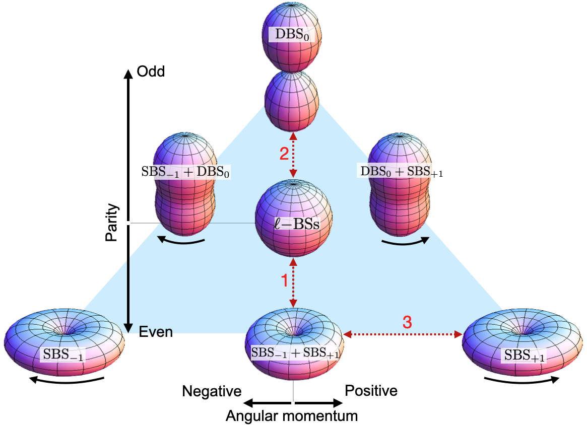
Figure 1: $\ell=1$ BSs family.

For each of the five types of solutions described above, there is a 1-dimensional family of BSs with $w_{\rm min}<w<\mu$, where $w_{\rm min}$ is family dependent. In an ADM mass, $M$ $vs.$ frequency $w$ diagram, they describe a spiral-type curve (costumary for BSs) - Fig.2 . As the frequency is decreased from the maximal value, $\mu$, the ADM mass increases up to a maximum value $M^{\rm(max)}$ which is family dependent. The energy density distribution of the solutions is illustrated by the morphologies in Fig. 1.

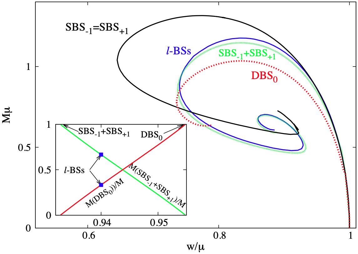
Figure 2: ADM mass $vs.$ frequency for some of the single-frequency limits of the $\ell=1$ BSs family. (Inset) Fraction of the total mass in SBS_-1+SBS₊₁ and in DBS₀ along the static sequence 1+2 in Fig. 1 for $w_{2}=0.94\mu$ (and $w_{1}/\mu=w_{3}/\mu$ in the $x$-axis).

The multi-frequency, multi-field interpolations. Relaxing the equal frequency requirement a larger solution space emerges (blue triangle in Fig. 1). There are multi-frequency BSs interpolating between the single-frequency ones, which are particular points in a manifold of solutions . As an illustration consider the interpolation SBS_-1+SBS₊₁ $\longleftrightarrow$ DBS₀, which goes through an $\ell$-BS. Fix, $e.g.$, $w_{2}=0.94\mu$ for the $\ell$-BS along the sequence - Fig. 2 (inset). On the one hand, decreasing $w_{1}=w_{3}$ ($w_{2}$ fixed), the toroidal static BS (SBS_-1+SBS₊₁) is approached for $w_{1}=w_{3}\simeq 0.933\mu$ - sequence 1 in Fig. 1. On the other hand, increasing $w_{1}=w_{3}$ ($w_{2}$ fixed), the dipole DBS₀ is obtained for $w_{1}=w_{3}\simeq 0.955\mu$ - sequence 2. These are static BSs sequences; thus $W=0$.

Similar interpolations occur between configurations with and without angular momentum, as in the transition SBS_-1+SBS₊₁ $\longleftrightarrow$ SBS₊₁ - sequence 3 in Fig. 1. Starting from a static, toroidal BS with $w_{1}=w_{3}=0.8\mu$, varying $w_{3}$ ($w_{1}$ fixed), the amplitude of $\Phi^{(1)}$ vanishes for a critical value of $w_{3}\simeq 0.829\mu$, yielding the single-field SBS₊₁. All intermediate solutions with $w_{1}\neq w_{3}$ possess a nonvanishing angular momentum. In all sequences, a similar picture holds considering other frequencies.

The manifold of solutions of the $\ell=1$ BSs family is as follows. Starting from an $\ell$-BS with a fixed frequency $w_{1}=w_{2}=w_{3}$, the line of static $(J=0)$ BSs is obtained keeping $w_{1}=w_{3}$ and varying the ratio $y\equiv w_{1}/w_{2}$ ($=w_{3}/w_{2}$). Then $y\in[y_{\rm min},y_{\rm max}]$. $y$ varies the parity of the BSs; the boundary values are the parity even and odd solutions, respectively. Then, for each fixed $y$ one can vary $x\equiv w_{3}/w_{1}$, with $x\in[x_{\rm min},x_{\rm max}]$, where the limits are $y$-dependent. $x$ varies $J$; for $x>1$ ($x<1$), $J$ is positive (negative) . Finally, varying the frequency of the starting $\ell$-BS yields a 3D manifold of solutions. Thus, we expect a $(2\ell+1)$D manifold of multi-frequency, multi-field BSs for a model with $(2\ell+1)$ complex scalar fields, including $\ell$-BSs as symmetry-enhanced solutions.

Dynamical (in)stability. We assess the dynamical stability of representative solutions in the $\ell=1$ BS family by resorting to fully non-linear dynamical evolutions of the corresponding Einstein–(multi-)Klein-Gordon system. The infrastructure used in the numerical evolutions is the same as in Sanchis-Gual et al. (2019).

Fig. 3 exhibits the results for a sequence of static solutions ($i.e.$ along sequences 1 and 2 in Fig. 1, including the dipole, the $\ell$-BS and the toroidal static BS). We find that all solutions (except the $\ell-$BS) are dynamically unstable, decaying to a multi-field BS in which all fields have $\ell=m=0$. Including $J$ does not improve dynamical stability. The SBS_±1 are unstable against a non-axisymmetric instability Sanchis-Gual et al. (2019) and all hybrid cases we have studied (such as SBS${}_{\pm 1}+$DBS₀) also decay to the fundamental $\ell=0$ BSs.

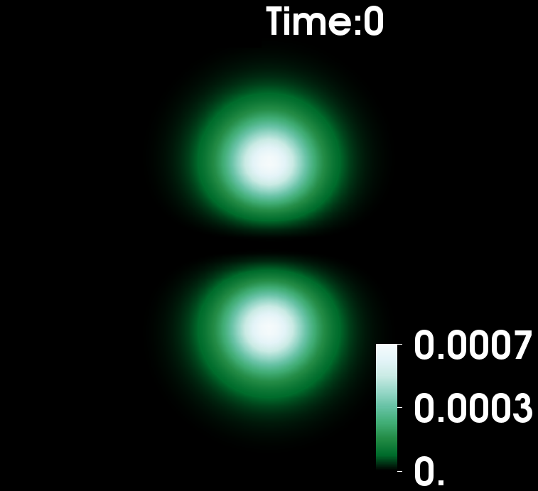
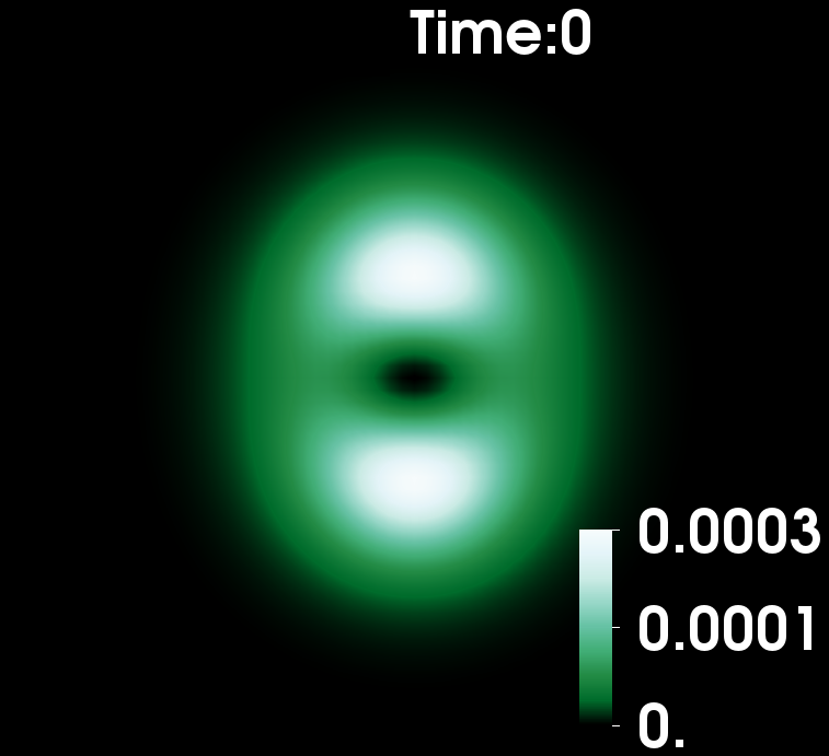
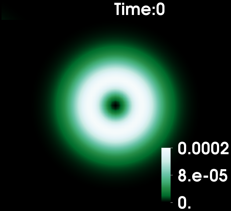
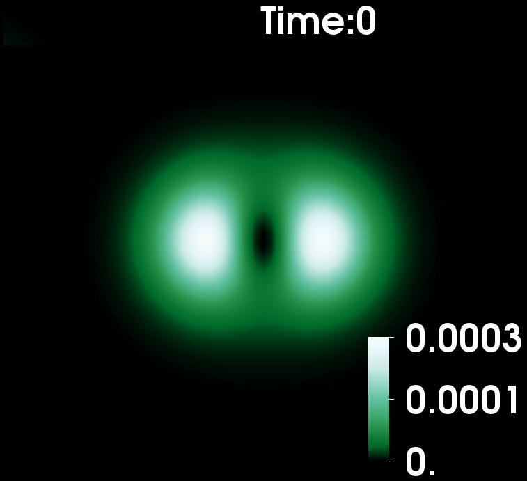
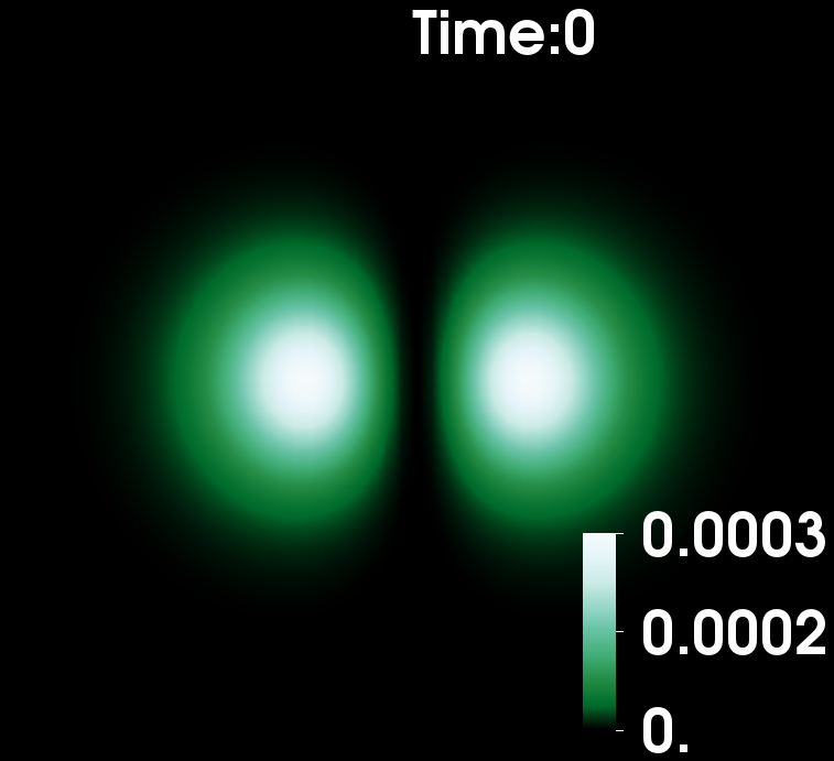
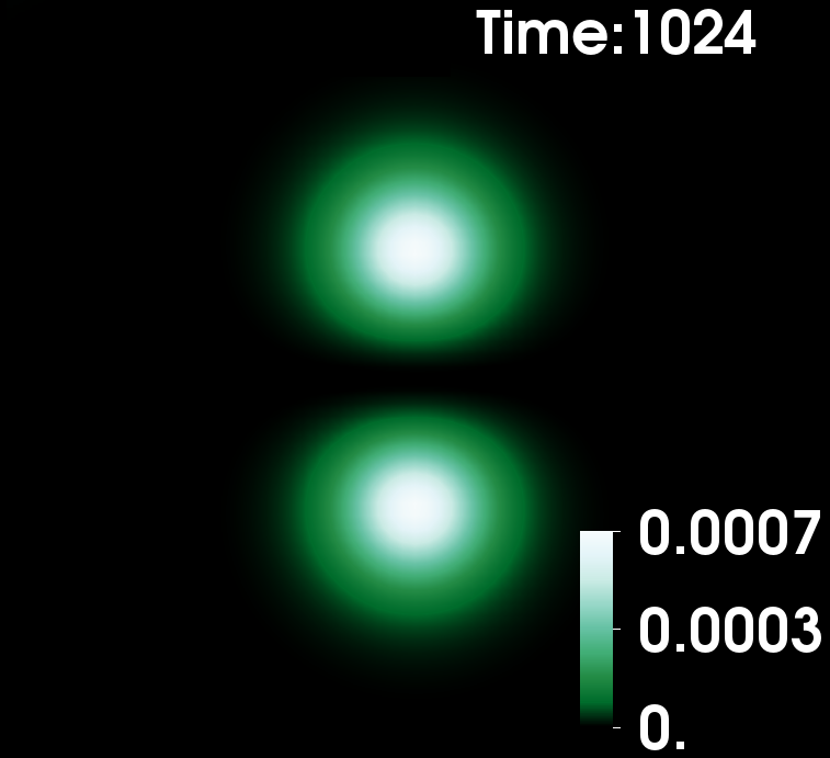
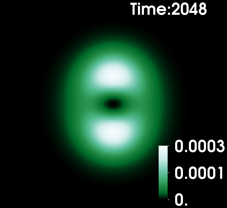
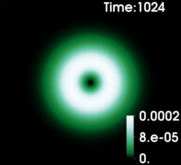
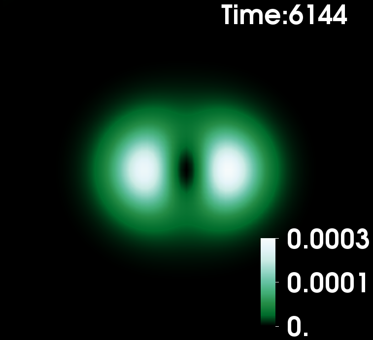
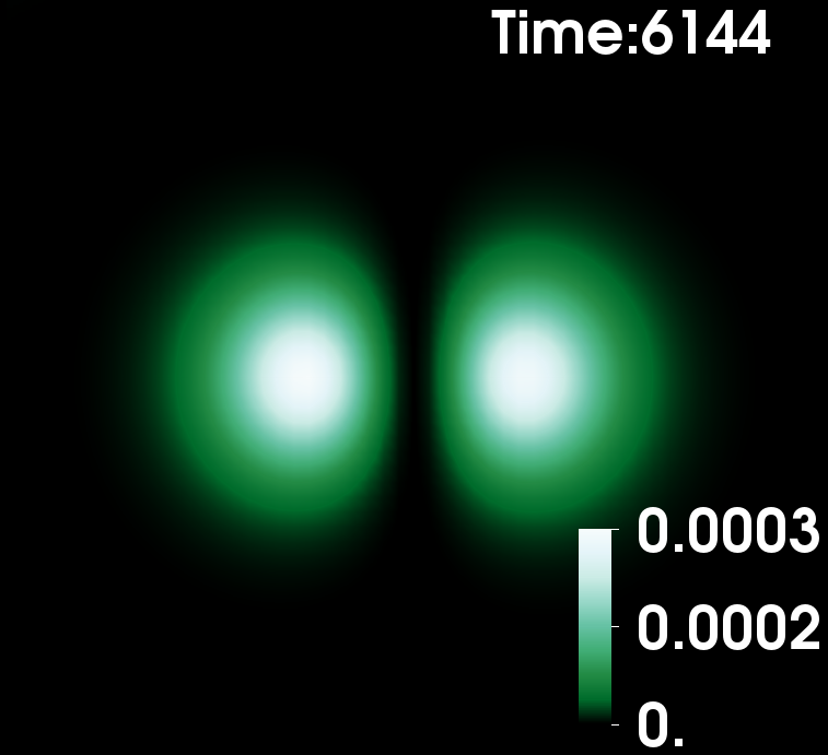
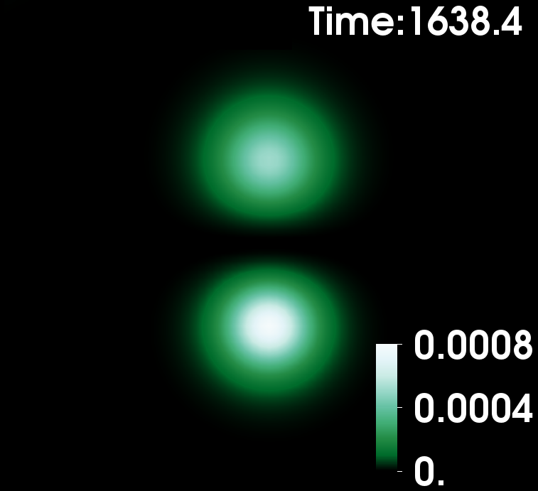
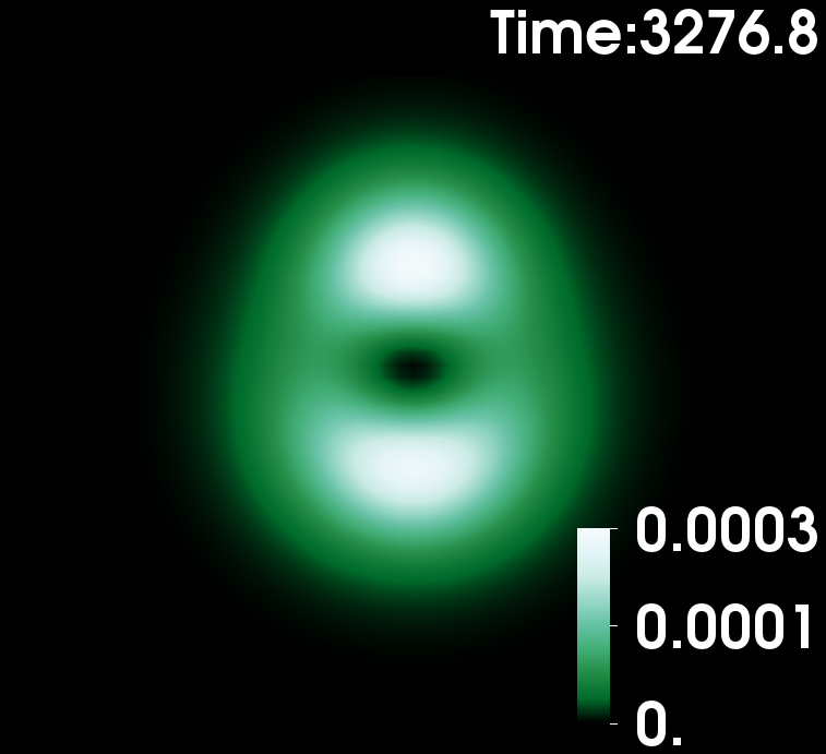
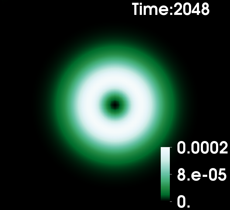
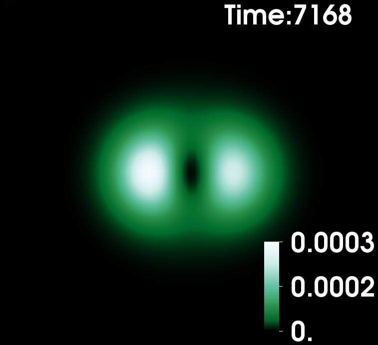
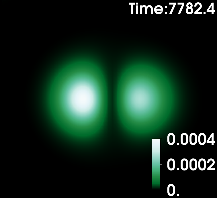
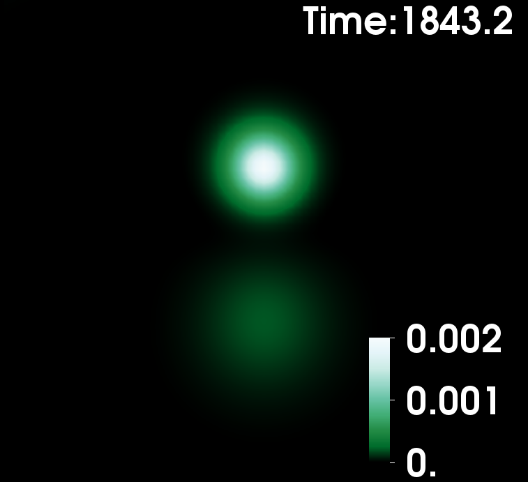
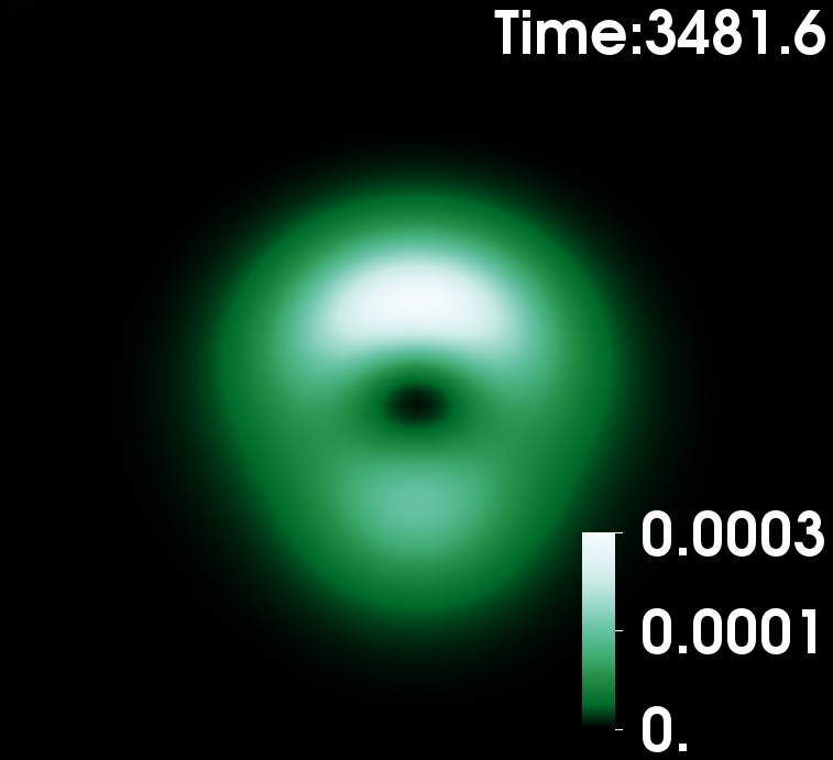
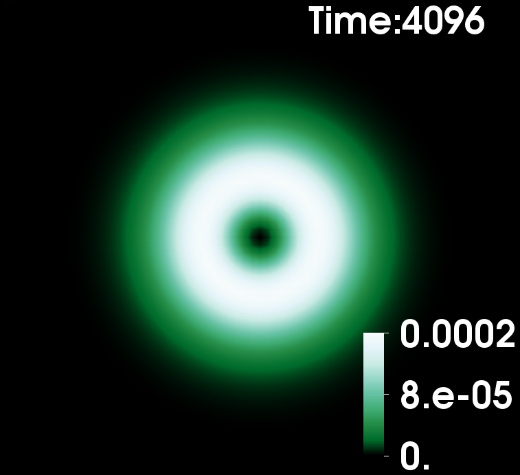
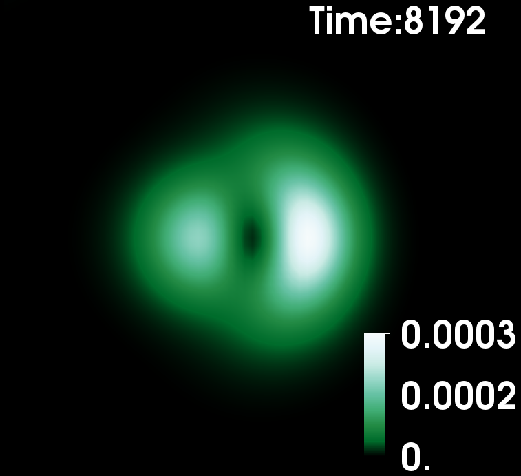
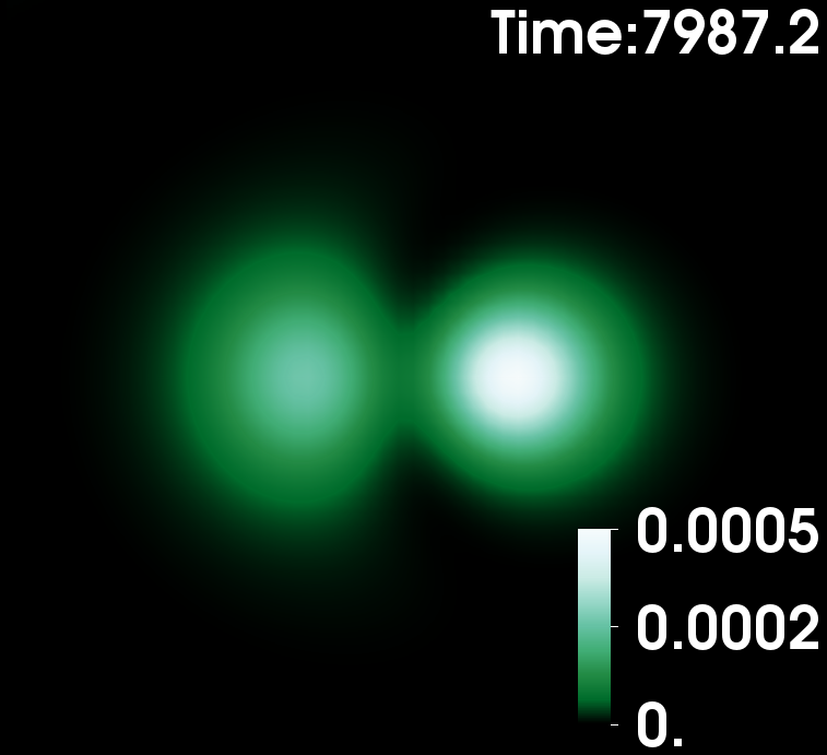
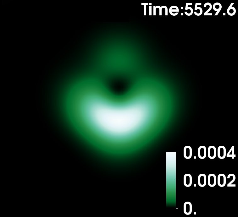
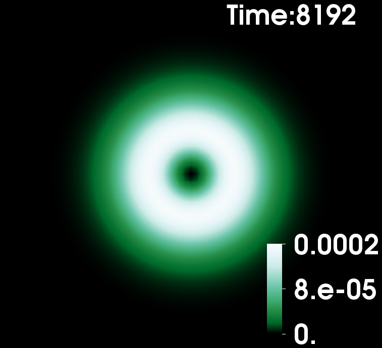
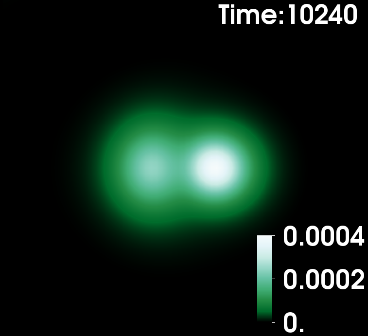
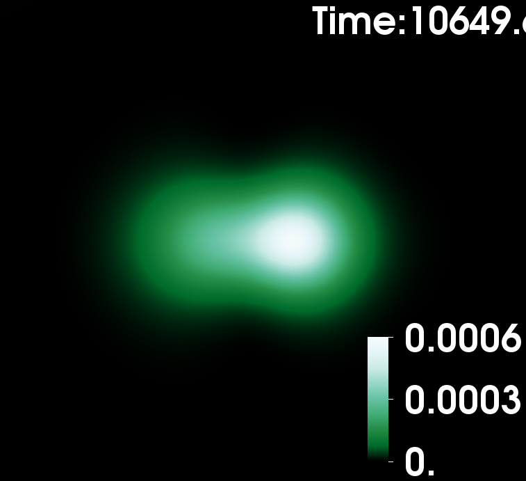
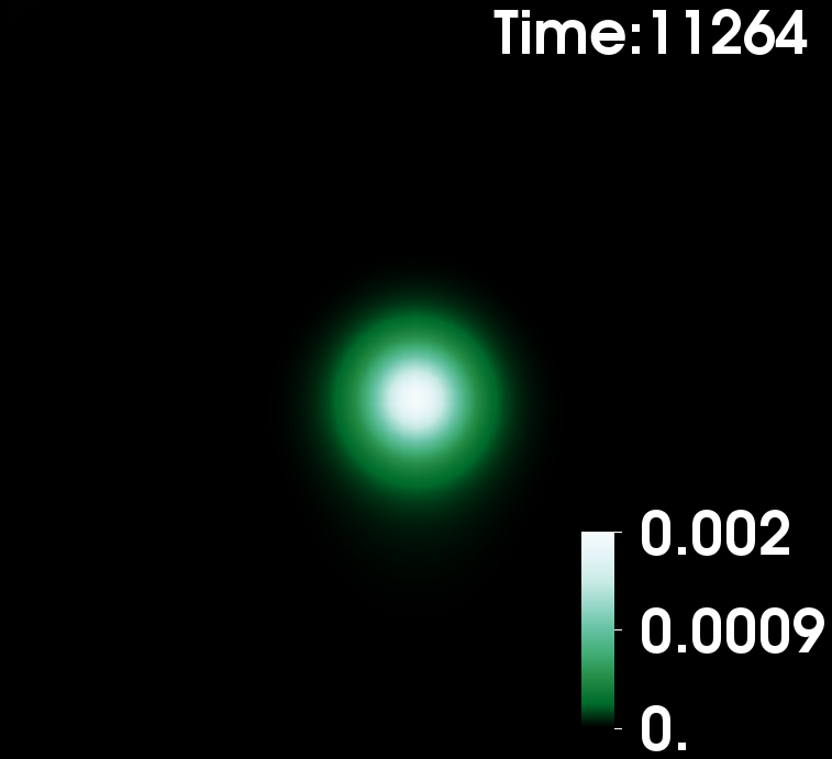
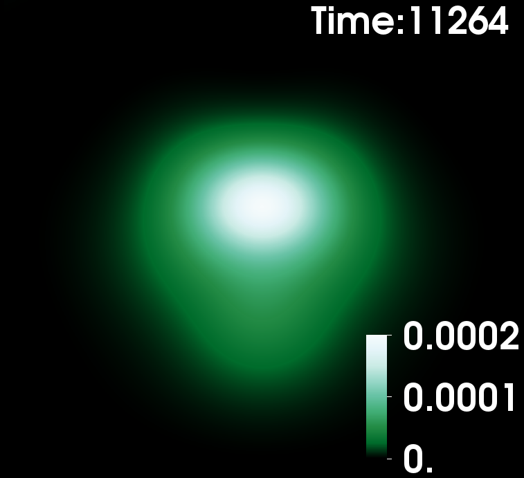
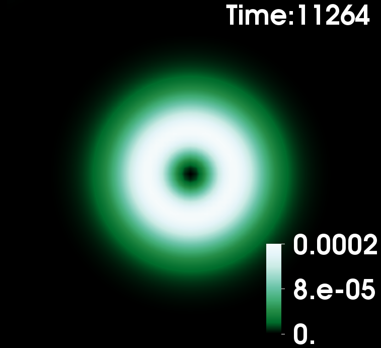
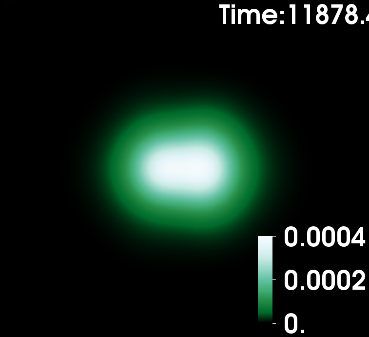
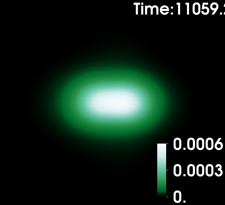
Figure 3: Time evolutions of the energy density for five static BSs in the $\ell=1$ family. Each column shows six sequential snapshots of the $xz$ ($y$=0) plane (time running from top to bottom). From left to right the values of $w_{1}=w_{3}$ of the five models are: 0.955 (DBS₀), 0.945, 0.940 ($\ell-{\rm BS}$), 0.935, 0.933 (${\rm SBS}_{-1}+{\rm SBS}_{+1}$).

Hybrid $\ell$-BSs and a stabilization mechanism. Instead of focusing on a single $\ell$-BSs family we now allow superpositions of such families with different $\ell$’s. The most elementary example is to add $\ell=0$ BSs to the $\ell=1$ family. Thus we add a fourth complex scalar field $\Phi^{(0)}$, obeying (1) and (2) with $j=0$ (hence, now $j=0,1,2,3$) and $m_{j}=0$. Its boundary conditions are $\partial_{r}\phi_{0}\big{|}_{r=0}=\phi_{0}\big{|}_{r=\infty}=\partial_{\theta}\phi_{0}\big{|}_{\theta=0,\pi}=0$, besides being parity even. Keeping only $\Phi^{(0)}$, the basic solution is the single-field, fundamental, monopole BS (MBS₀). We now show that adding MBS₀ can quench the instabilities observed in the $\ell=1$ family.

To be concrete we consider the following superpositions: $(A)$ MBS₀+SBS₊₁ and $(B)$ MBS₀+DBS₀. As an illustration of $(A)$, fixing $w_{3}/\mu=0.98$, there is a continuous sequence of solutions reducing to the MBS₀ (SBS₊₁) for $w_{0}/\mu=0.964$ (0.975). We refer to the intermediate configurations as ‘Saturns’. Their dynamical evolutions - Fig. 4 - exhibit a simple pattern: sufficiently close to the MBS₀ (SBS₊₁) limit, Saturns are stable (unstable). Here, stability means no sign of instabilities for long evolutions ($t\simeq 24000$) . Attempting to interpret the transition between the two regimes, we observe a correlation between instability and the $r$ coordinate of the maximum of the energy density - Fig. 5: when the latter is at the origin ($r=0$) no instability is observed.

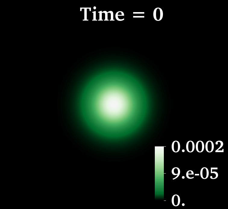
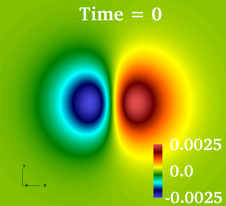
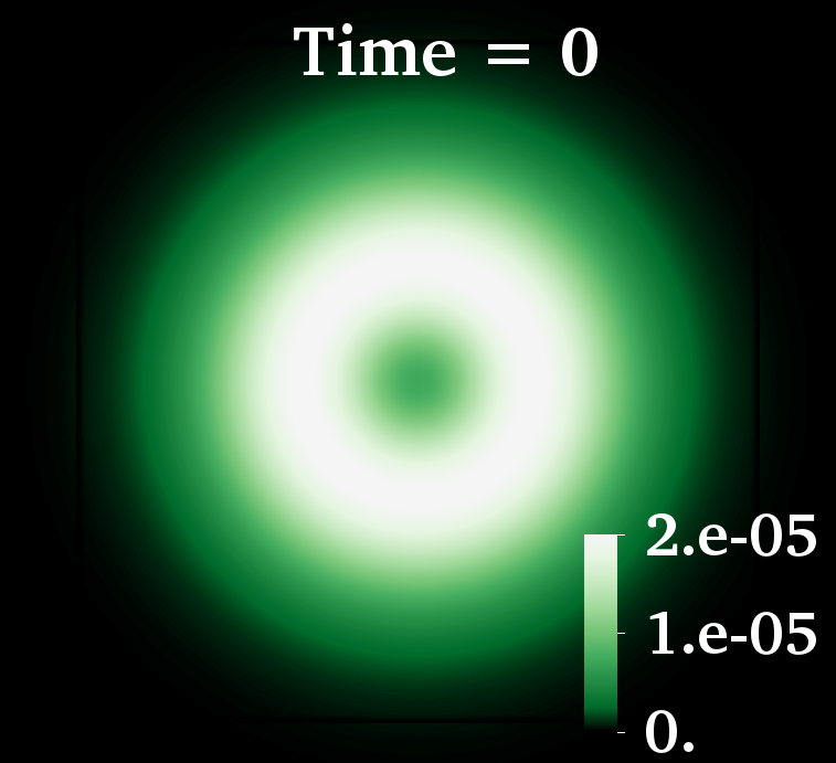
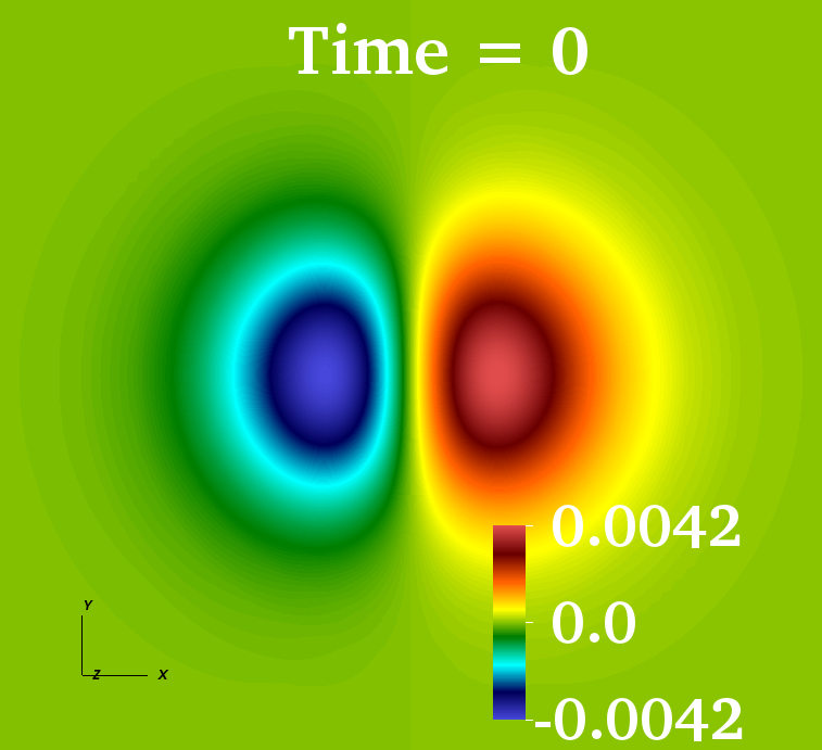
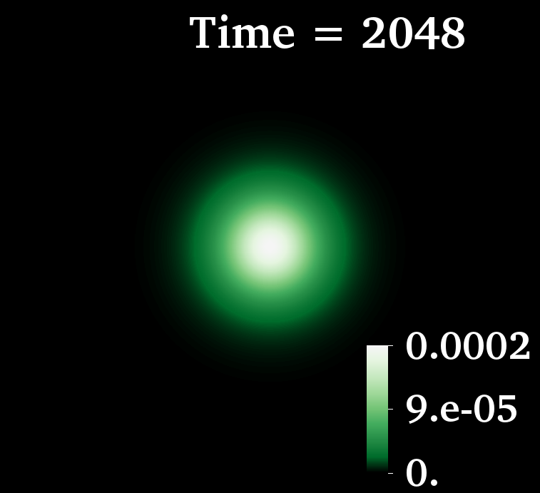
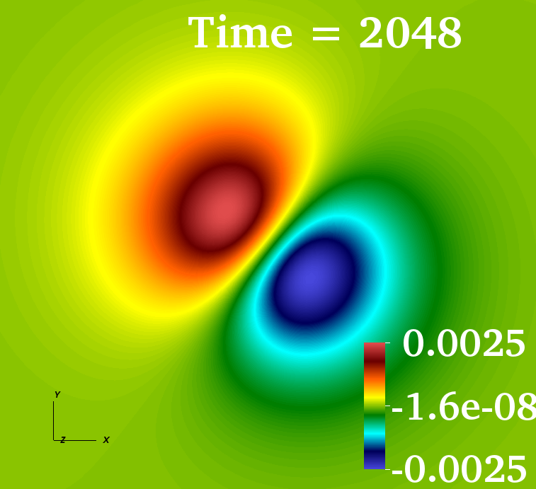
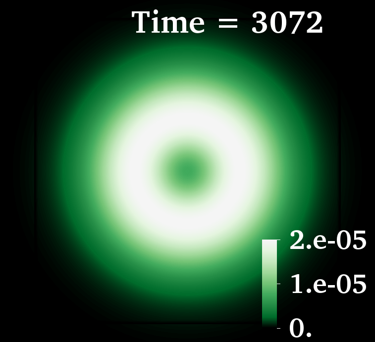
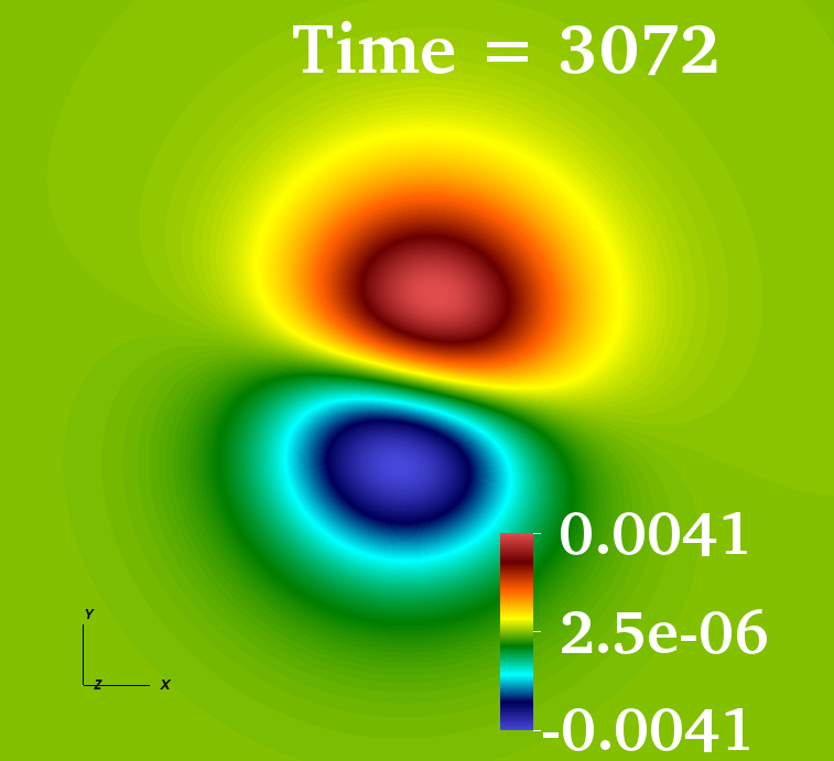
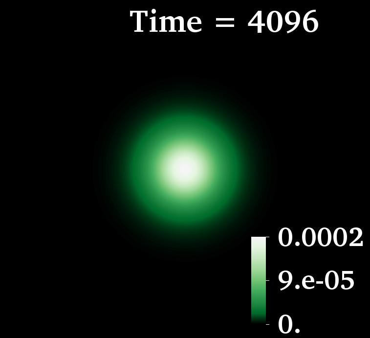
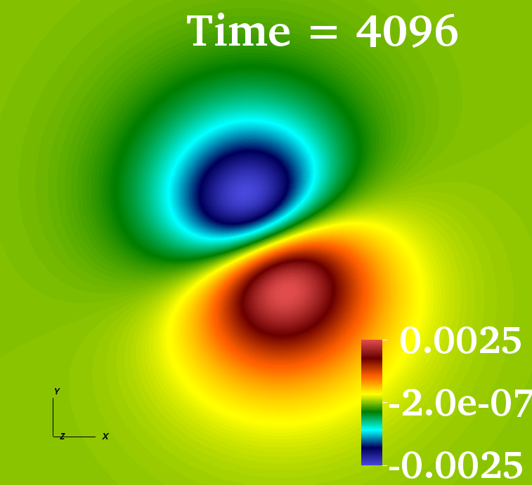
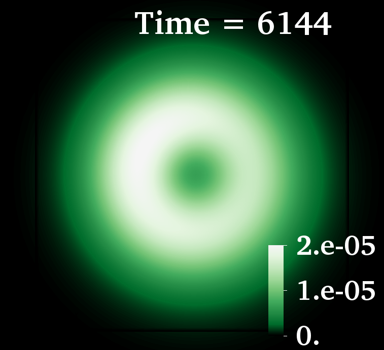
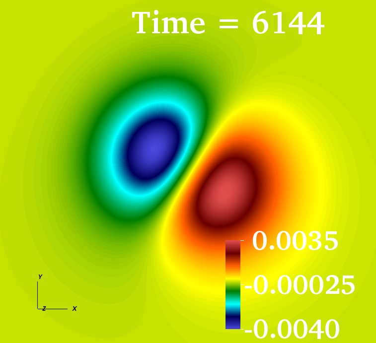
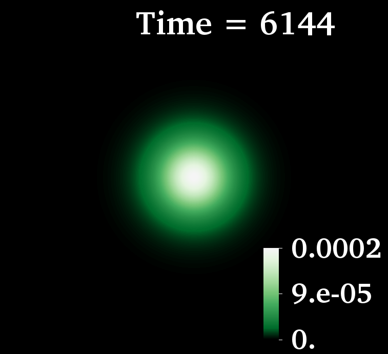
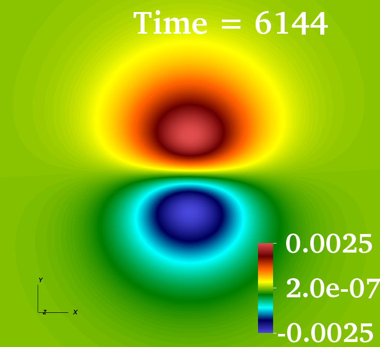
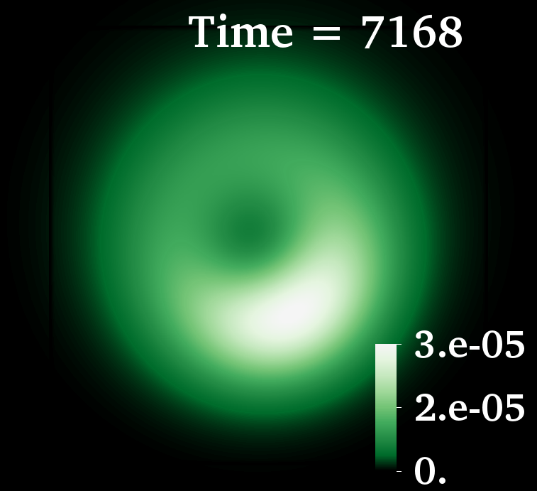
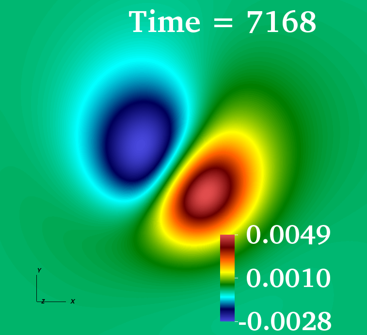
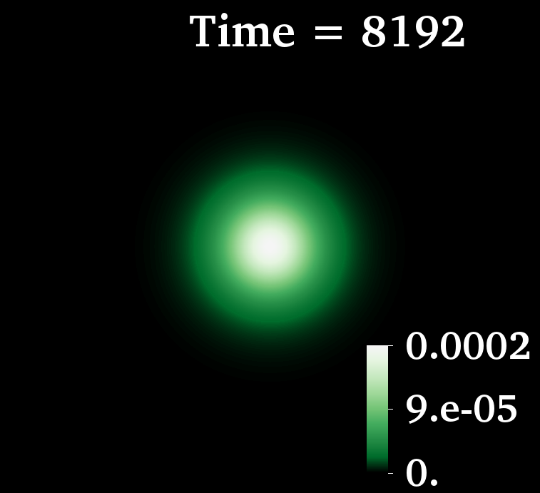
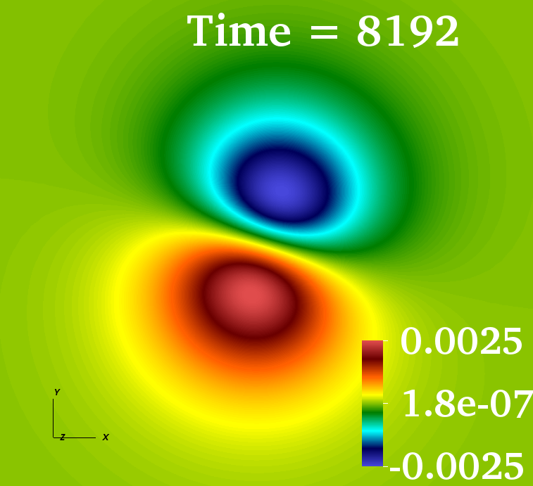
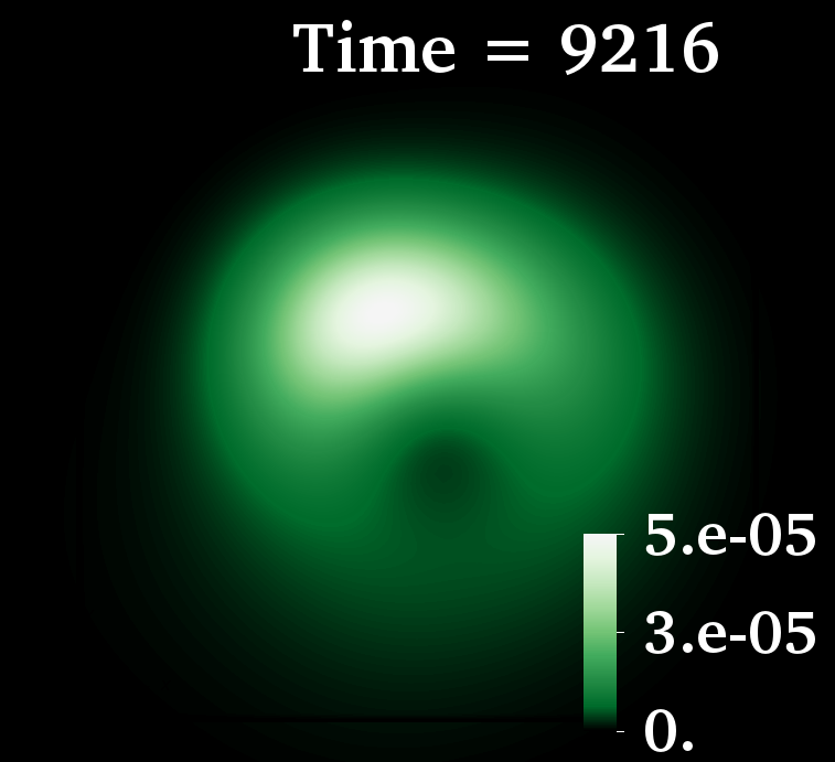
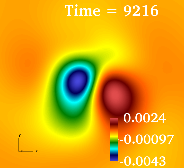
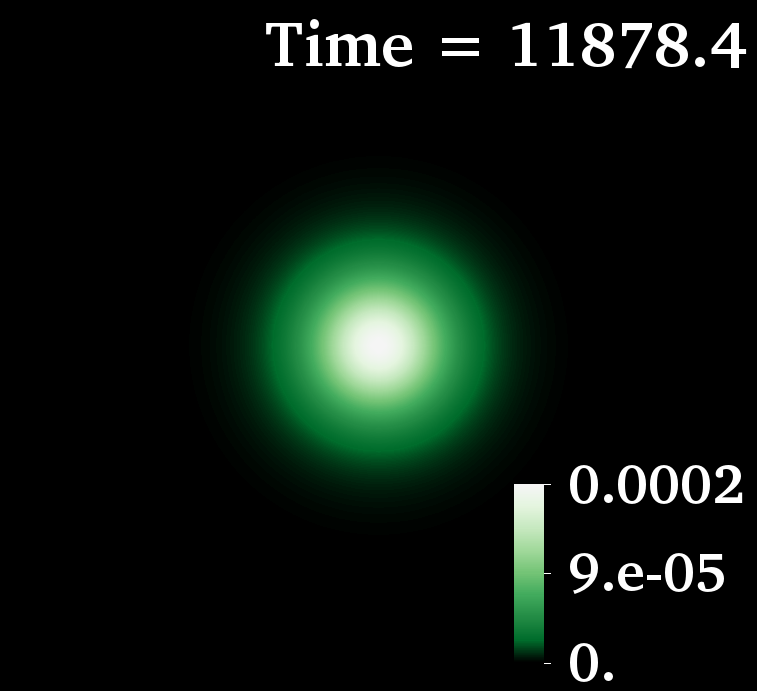
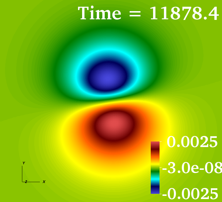
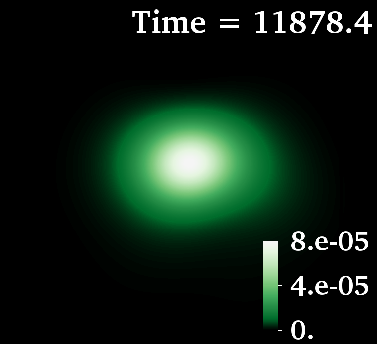
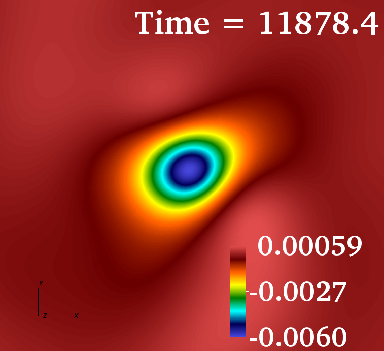
Figure 4: Time evolution (top to bottom) of two Saturns: (left and middle left) $\omega_{1}/\mu=0.967$; (middle right and right) $\omega_{1}/\mu=0.974$. For each case the energy density and the real part of $\Phi^{(3)}$ on the $xy$ plane are shown. The first (second) Saturn is close to MBS₀ (SBS₊₁) and is stable (unstable).

As an example of $(B)$, fixing $w_{0}/\mu=0.97$, there is a continuous sequence of solutions reducing to the MBS₀ (DBS₀) for $w_{2}/\mu=0.983$ ($0.973$). We refer to the intermediate configurations as ‘pods’. Evolving this sequence of pods reveals analogous patterns: $(a)$ sufficiently close to the MBS₀ (DBS₀) limit, pods are stable (unstable) - see Appendix A for snapshots of the evolutions; $(b)$ when the energy density maximum, which, in general, has two symmetric points located on the $z$-axis (i.e, $\theta=0,\pi$) is at the origin, no instability is observed. - Fig. 5 (inset).

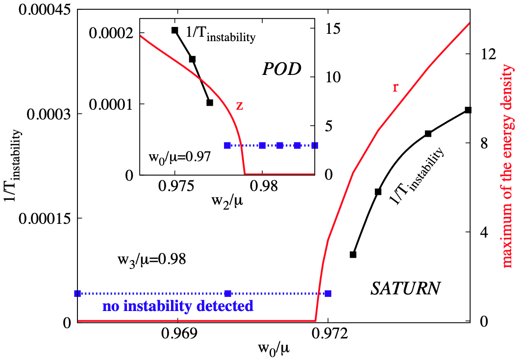
Figure 5: Instability timescale (black dots and lines) and maximum of the total energy density (red lines) for the sequence of Saturns (main panel) and pods (inset) described in the text. The blue points and line are thresholds when no instability is seen. The $z$ coordinate in the inset is $r$ for $\theta=0,\pi$. $T_{\rm{instability}}$ refers to the time when we observe that the solution begins to clearly deviate from axisymmetry for Saturns and from equatorial symmetry for pods.

Generality and remarks. An analogous family of vector $\ell=1$ BSs should exist. Preliminary results show an important difference: the whole sequence 3 (see Fig. 1) is stable in the vector case, including the SBS_-1+SBS₊₁ static configuration, which is now spheroidal rather than toroidal (see Appendix B for details). This is a consequence of the stability of vector SBS_±1 Sanchis-Gual et al. (2019). On the other hand, we have evidence that the vector DBS₀ is unstable, as in the scalar case (see Appendix C).

A byproduct of our construction is the realization that all single-frequency BSs arising in (combinations of) models of type (1) are continuously connected within a multidimensional solutions manifold, interpolated by multi-frequency solutions. For instance, spherical (MBS₀) and spinning (SBS_±1) BSs, typically described as disconnected, are connected (via Saturns).

Adding the fundamental MBS₀, which is the ground state of the whole family, stabilizes different types of unstable BSs, such as excited monopole BSs Bernal et al. (2010), spinning and dipole BSs. Such stable configurations can actually form from the (incomplete) gravitational collapse of dilute distributions of the corresponding fields and multipoles - see Appendix C. It would be interesting to probe the generality of this cooperative stabilization mechanism, and if other (higher $\ell$, say) multipolar BSs can be stabilized similarly .

Another mechanism for mitigating instabilities is adding self-interactions Di Giovanni et al. (2020b), which was suggested to quench the instability of spinning BSs, without requiring the energy density to be maximized at the origin Siemonsen and East (2021). It would be interesting to construct the corresponding $\ell=1$ BSs family in models with self-interactions, and investigate whether other members of the family can be stabilized by self-interactions.

Acknowledgements. We thank Darío Núñez, Víctor Jaramillo, Argelia Bernal, Juan Carlos Degollado, Juan Barranco, Francisco Guzmán and Luis Ureña-López, for useful discussions and valuable comments. This work was supported by the Spanish Agencia Estatal de Investigación (grant PGC2018-095984-B-I00), by the Generalitat Valenciana (PROMETEO/2019/071 and GRISOLIAP/2019/029), by the Center for Research and Development in Mathematics and Applications (CIDMA) through the Portuguese Foundation for Science and Technology (FCT - Fundação para a Ciência e a Tecnologia), references UIDB/04106/2020 and UIDP/04106/2020, by national funds (OE), through FCT, I.P., in the scope of the framework contract foreseen in the numbers 4, 5 and 6 of the article 23, of the Decree-Law 57/2016, of August 29, changed by Law 57/2017, of July 19 and by the projects PTDC/FIS-OUT/28407/2017, CERN/FIS-PAR/0027/2019 and PTDC/FIS-AST/3041/2020. This work has further been supported by the European Union’s Horizon 2020 research and innovation (RISE) programme H2020-MSCA-RISE-2017 Grant No. FunFiCO-777740 and by FCT through Project No. UIDB/00099/2020. We would like to acknowledge networking support by the COST Action GWverse CA16104. Computations have been performed at the Servei d’Informàtica de la Universitat de València, the Argus and Blafis cluster at the U. Aveiro and on the “Baltasar Sete-Sois” cluster at IST.

Appendix A. Evolution of pods. In Fig. 6 we exhibit the time evolution of two illustrative pods, one stable and one unstable, along the sequence described in the main text, with $w_{0}/\mu=0.97$.

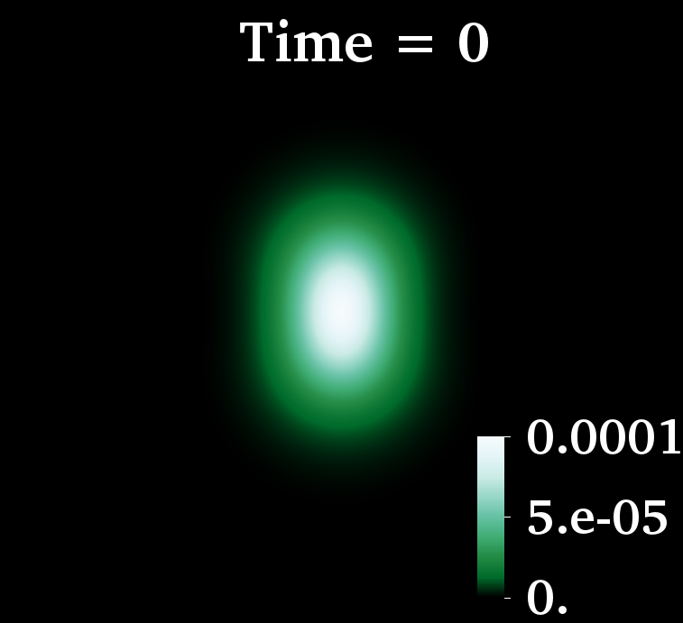
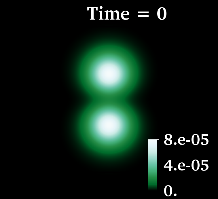
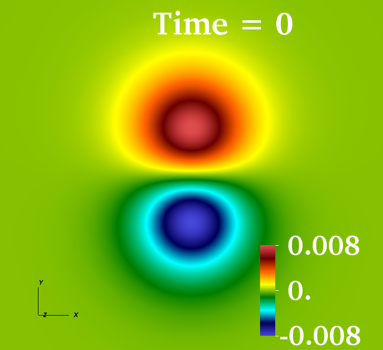
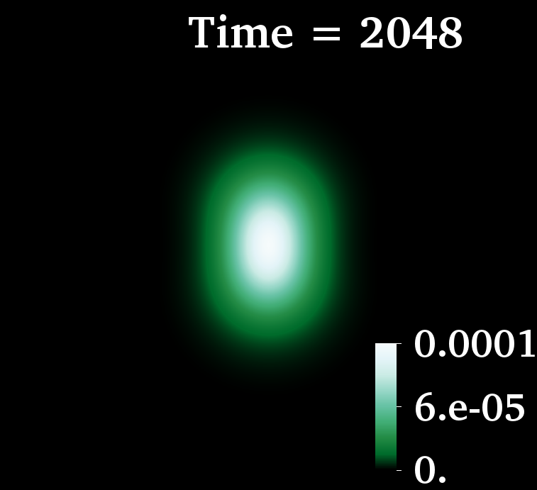
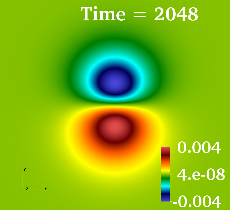
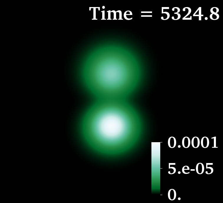
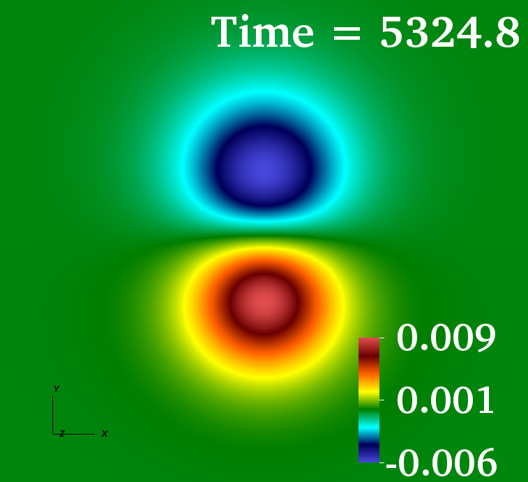
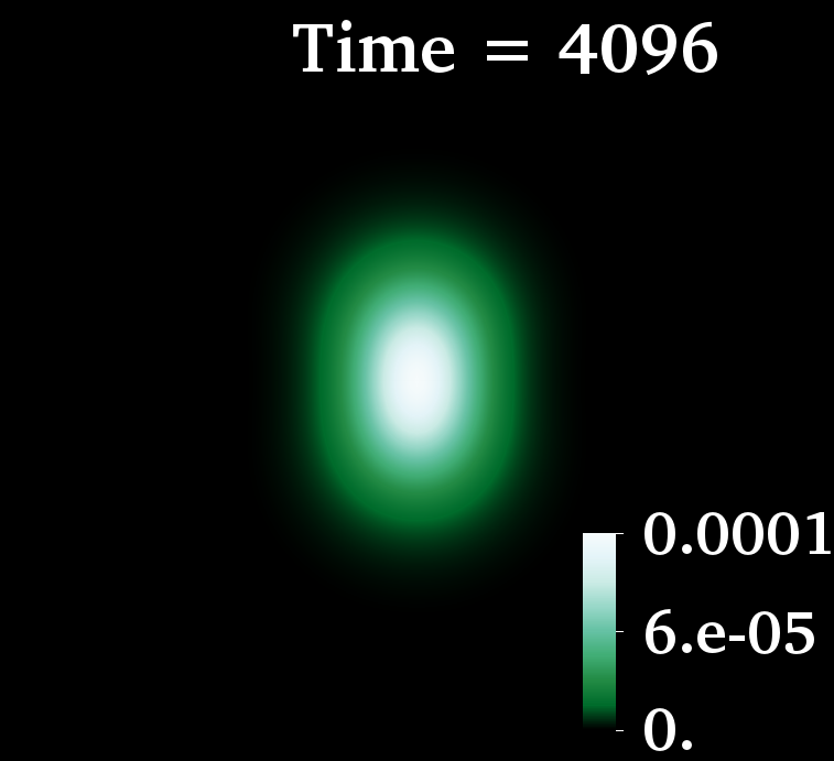
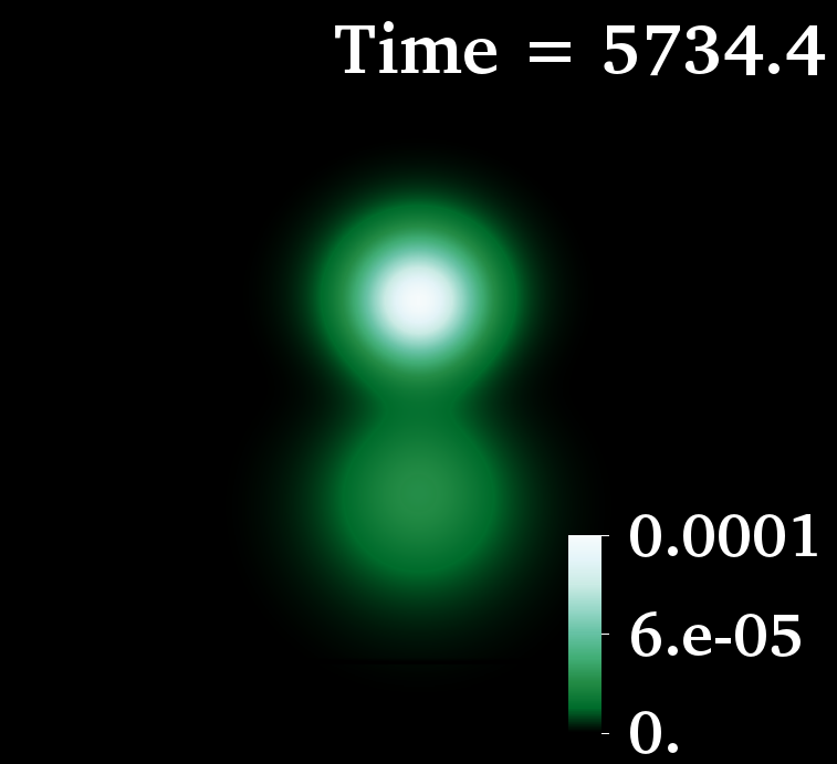
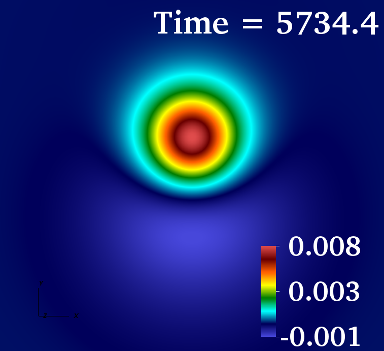
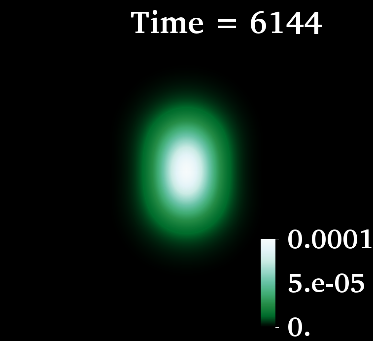
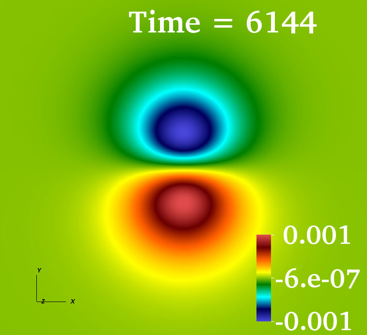
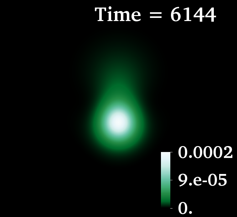
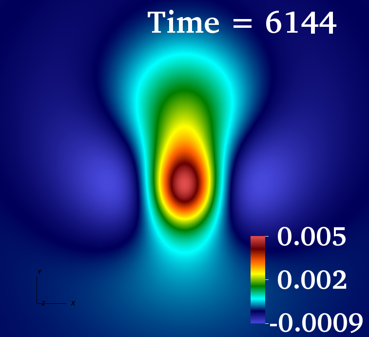
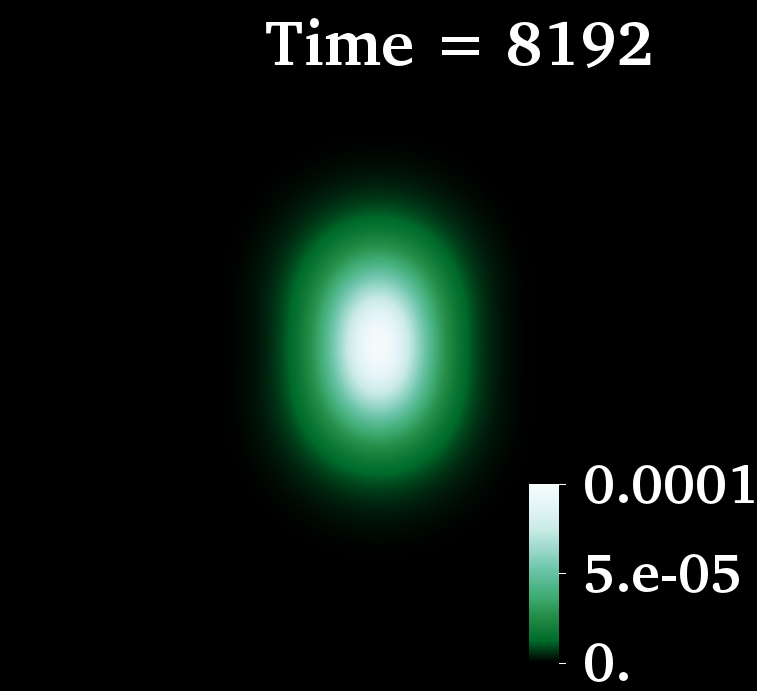
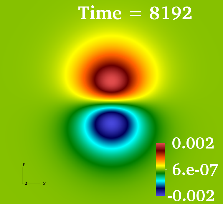
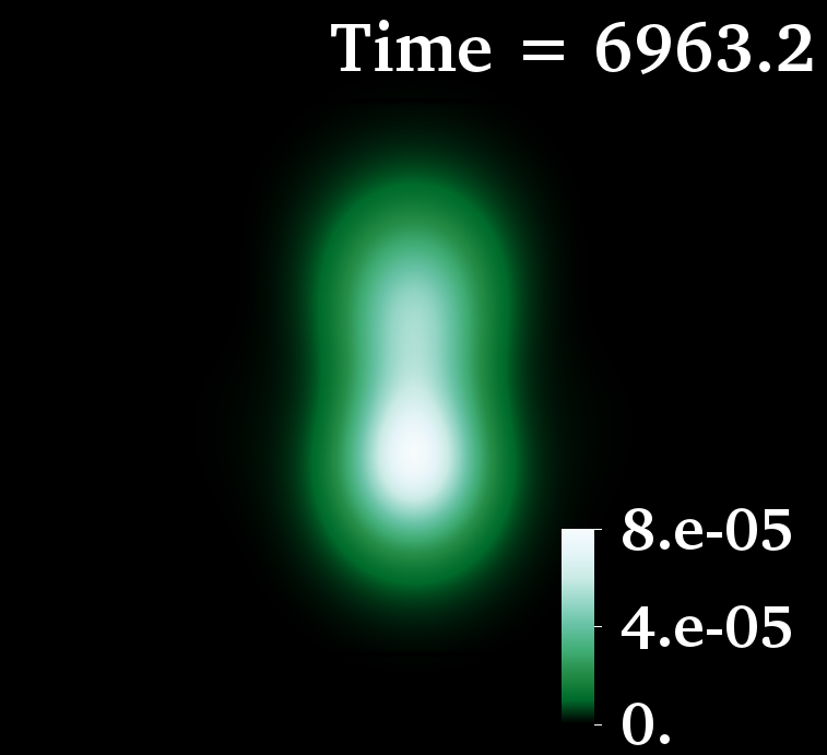
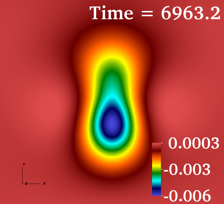
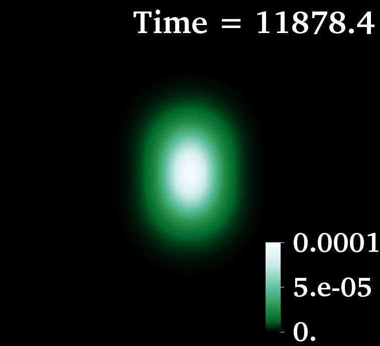
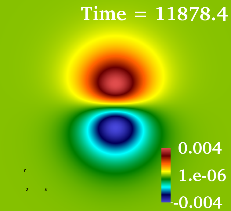
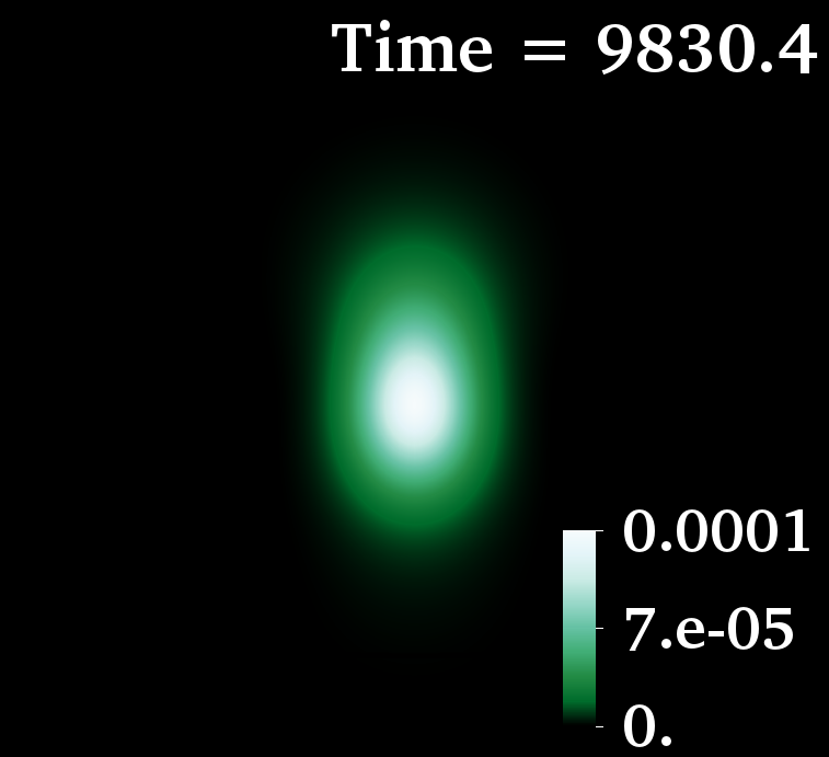
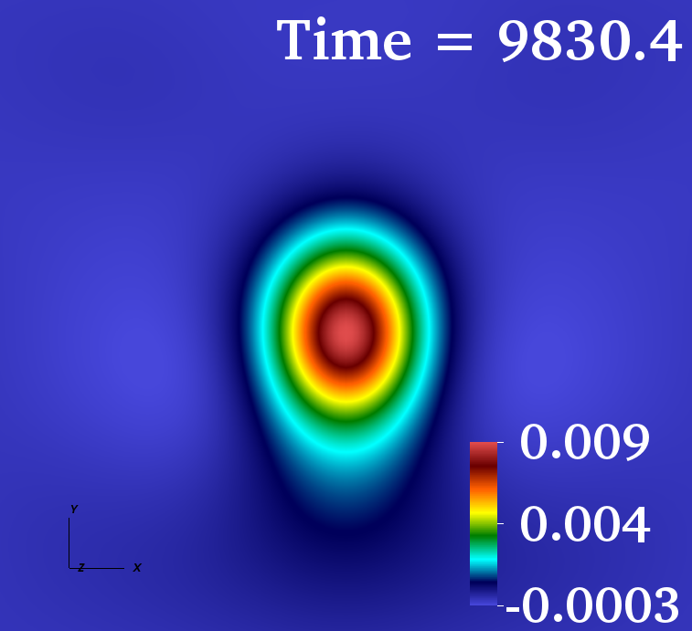
Figure 6: Time evolution (top to bottom) of two pods: (left and middle left) $\omega_{2}/\mu=0.98$; (middle right and right) $\omega_{2}/\mu=0.975$. For each case the energy density and the real part of $\Phi^{(2)}$ on the $xz$ plane are shown. The first (second) pod is close to MBS₀ (DBS₀) and is stable (unstable).

The decay of the unstable one is similar to the one of the pure dipoles, exhibited in Fig. 3 (left column). Observe that the decay of the unstable Saturns shown in Fig. 4, is triggered by a non-axisymmetric perturbation, inherited from the instability of the pure SBS_±1; this is not the case for the decay of the unstable pods, which would occur even in axi-symmetry.

Appendix B. Vector BSs evolutions. Dynamical evolutions of representative members of the $\ell=1$ family of vector BSs are performed using the same computational infrastructure of  Sanchis-Gual et al. (2019). The vector BSs (aka Proca) equations are solved using a modification of the Proca thorn in the Einstein Toolkit Witek et al. (2020); Zilhão et al. (2015) to include a complex field. Here we illustrate these evolutions with the vector SBS_-1+SBS₊₁ configuration, which we succeded in constructing, and it is static as in the scalar case but now spheroidal, a property inherited from the spheroidal nature of the spinning vector BSs (SBS_±1).

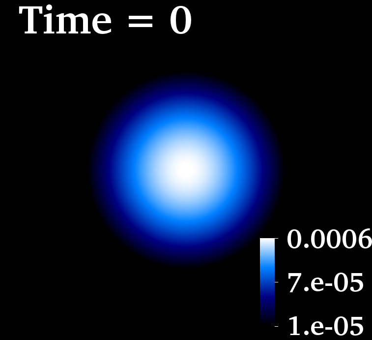
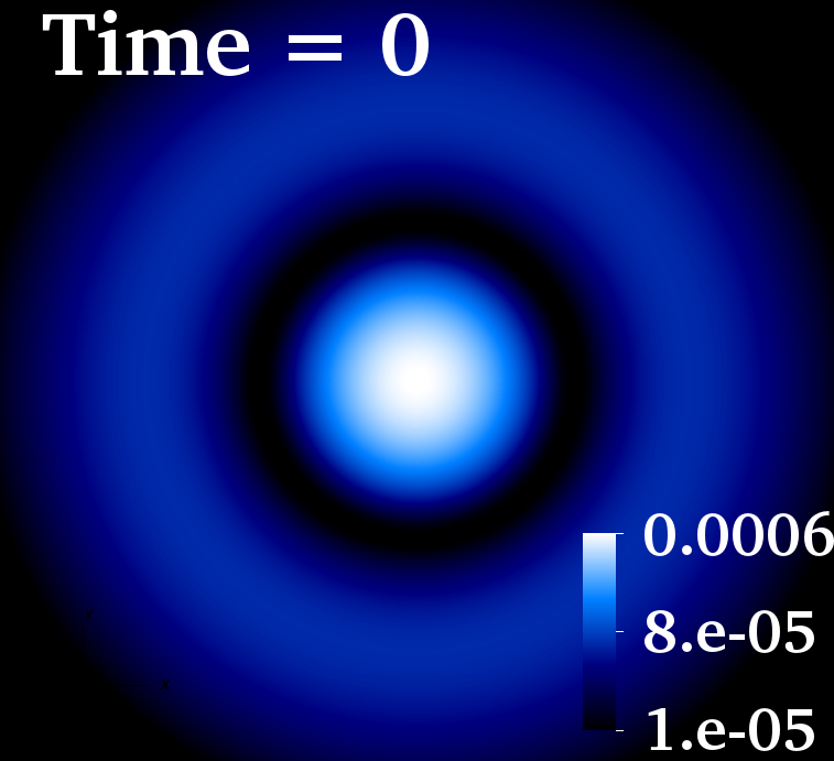
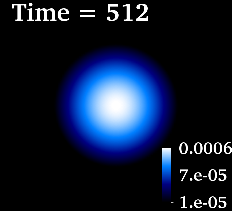
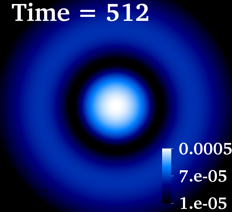
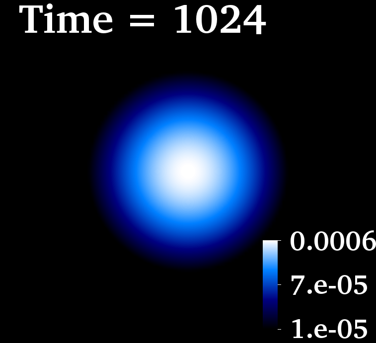
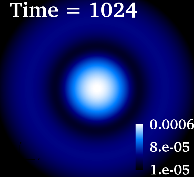
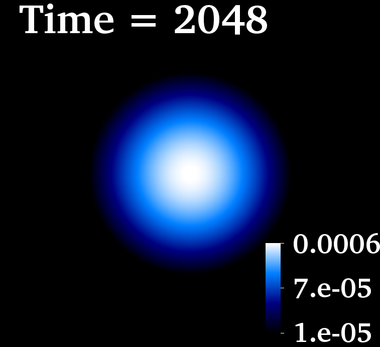
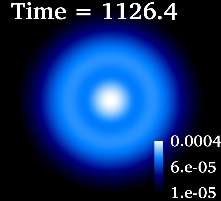
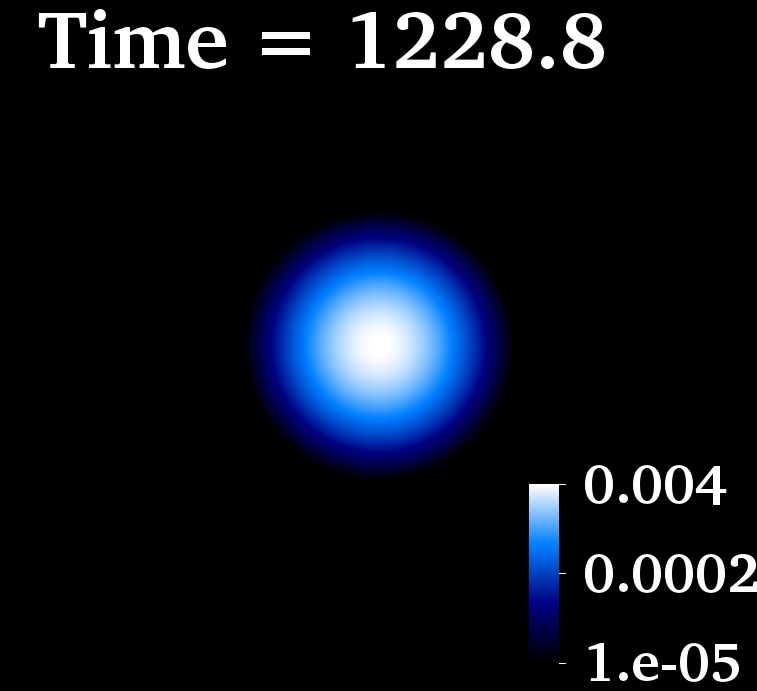
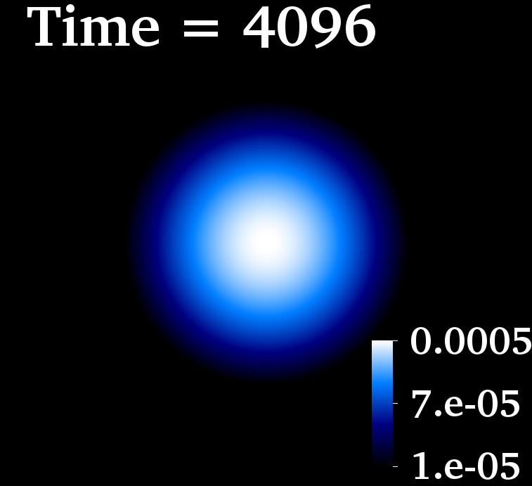
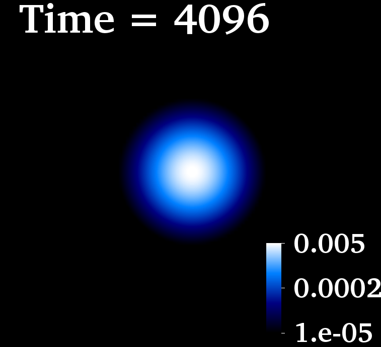
Figure 7: Time evolution (top to bottom) of two vector SBS_-1+SBS₊₁ with $\omega_{2}/\mu=0.95$. The fundamental (excited state) is shown in the left (right) column and is found to be stable (unstable).

As in the scalar case, the individual (complex, vector) fields carry angular momentum density, but the total angular momentum is zero. We observe that the vector SBS_-1+SBS₊₁ is dynamically stable - Fig. 7 (left column), as their individual components (SBS_±1) Sanchis-Gual et al. (2019). In Fig. 7 (right column) we also plot the time evolution of the energy density for one excited state (with one node) of the vector SBS_-1+SBS₊₁. This excited star decays to the nodeless solution. Interestingly, the maximum of the energy density of the fundamental solution is at the centre. These results indicate that the non-axisymmetric instability observed in spinning scalar BSs (as well as for the vector stars with $m>1$ Sanchis-Gual et al. (2019)) is also present in these multi-field BSs. Moreover, the same correlation observed in the main text for the scalar case applies to the vector case: the maximum of the energy density is at the centre for stable stars.

Appendix C. Dynamical formation. A further, complementary, confirmation of dynamical robustness is the existence of a formation mechanism. For the fundamental (monopole) BSs such mechanism exists: gravitational cooling Seidel and Suen (1994); Di Giovanni et al. (2018). We thus investigate the dynamical formation of some multi-field BSs from the collapse of an initial dilute cloud of bosonic fields. Our results show that the stable models can be formed through the gravitational cooling mechanism, while unstable models decay to the spherical non-spinning solutions, see Fig. 8.

Scalar
DBS0	Vector
DBS0	Scalar
DBS0+SBS+1	Vector SBS+1+SBS-1

($y=0$, $xz$ plane)

$|$

($z=0$, $xy$ plane)

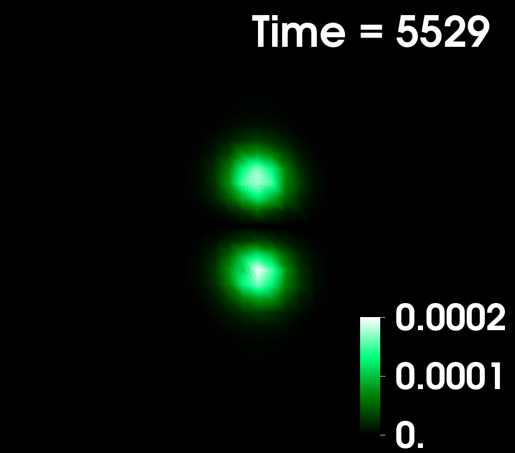
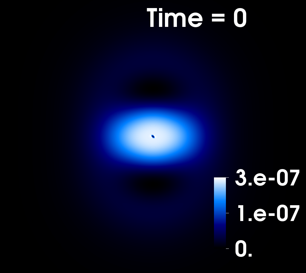
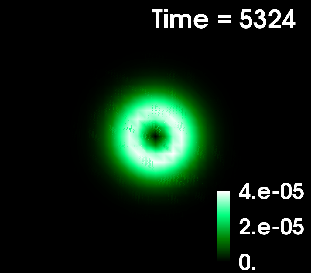
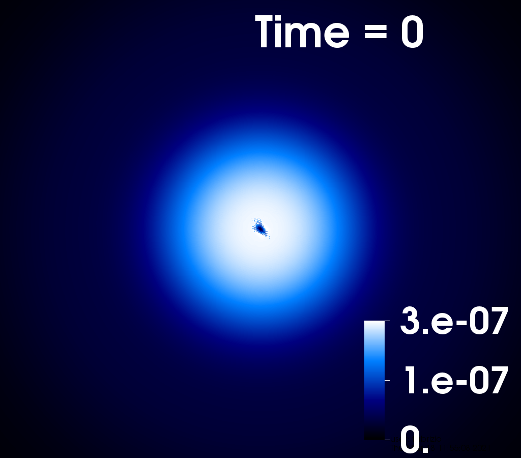
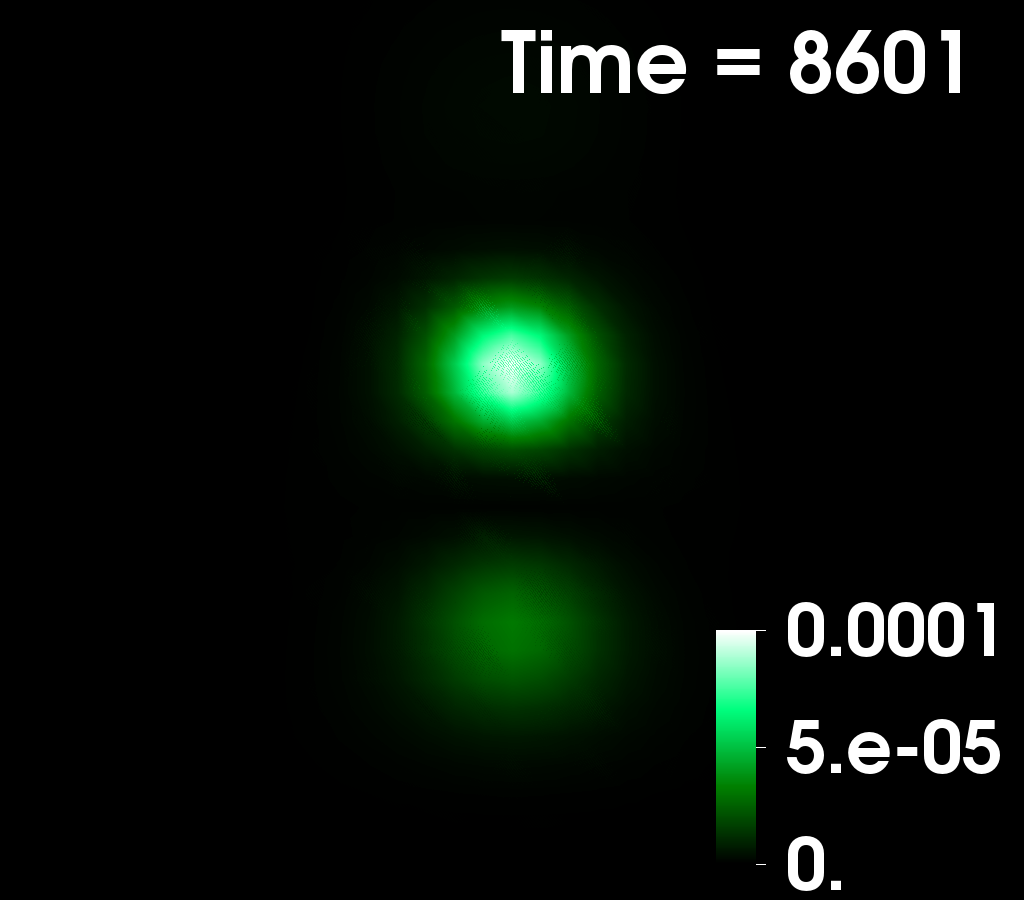
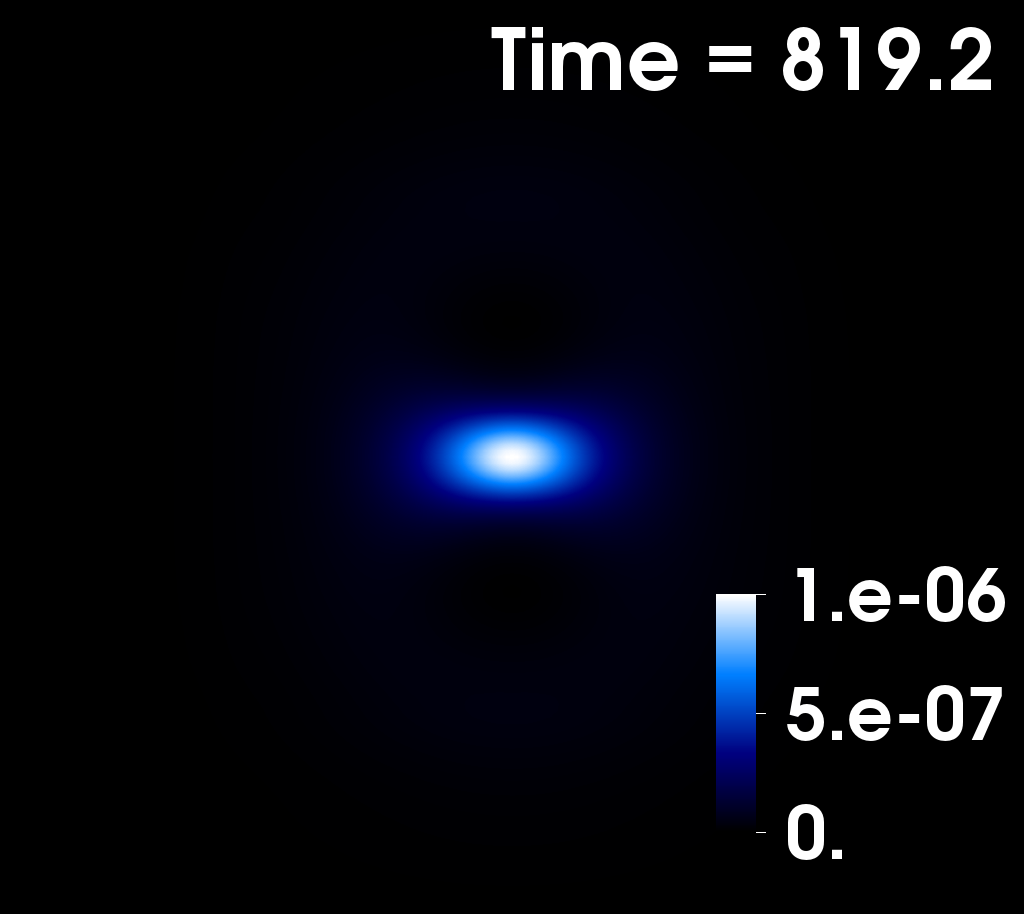
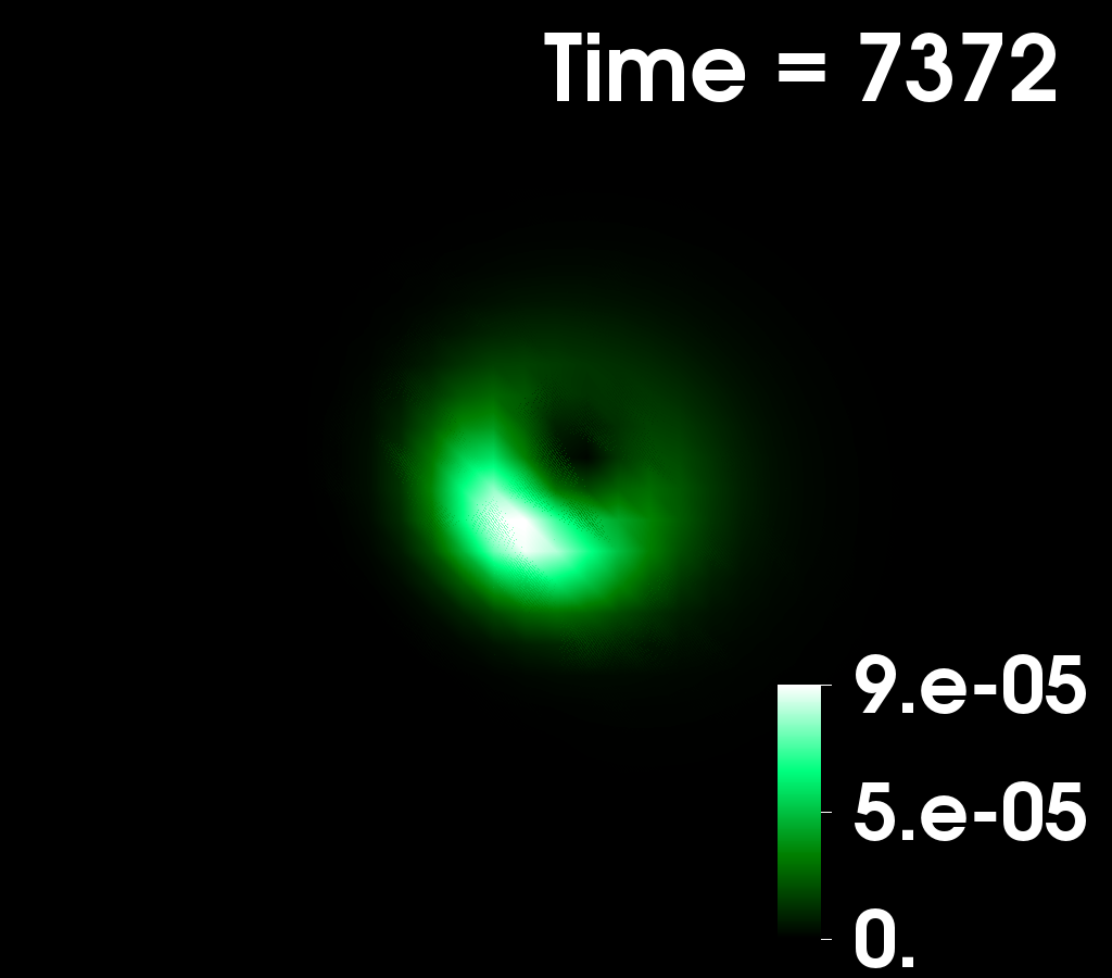
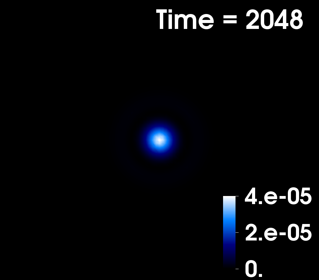
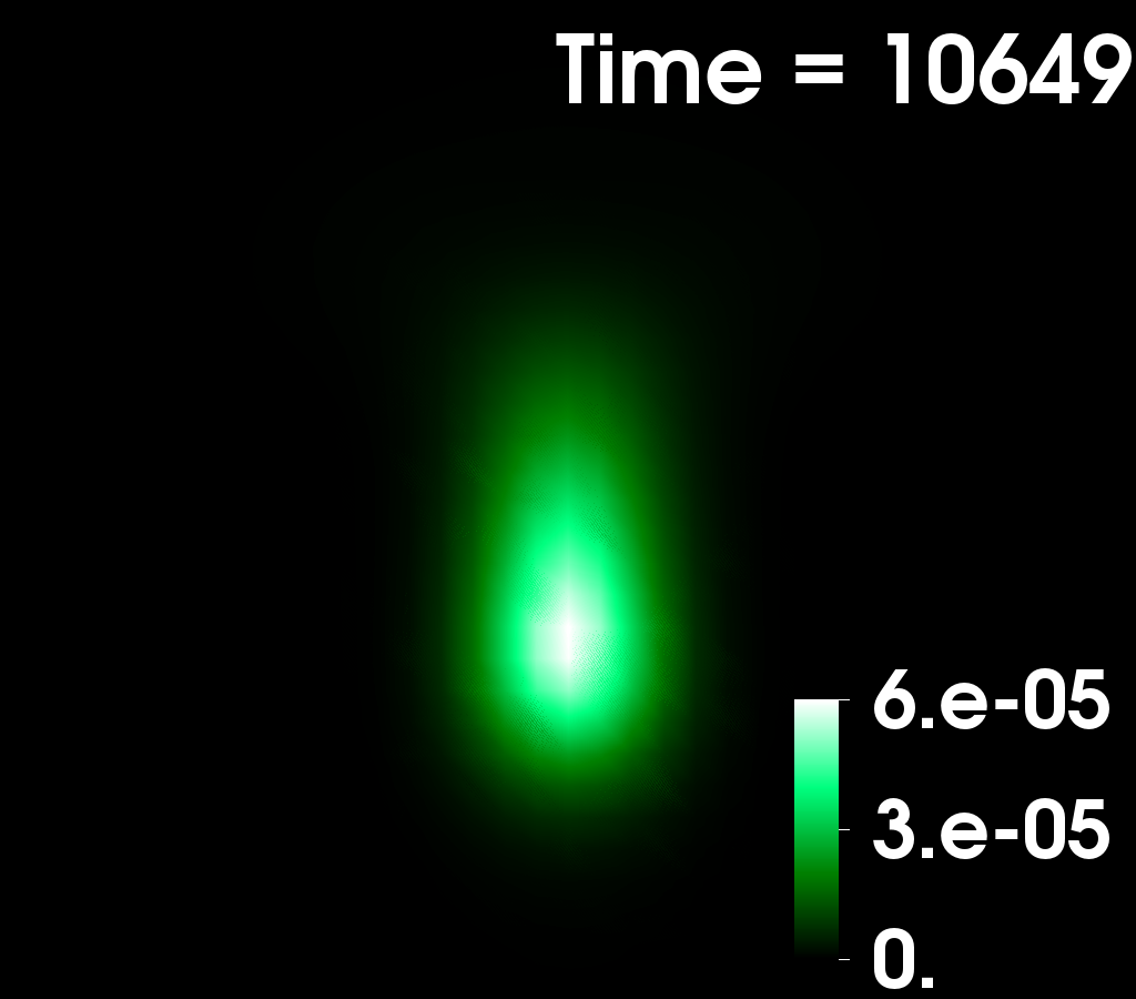
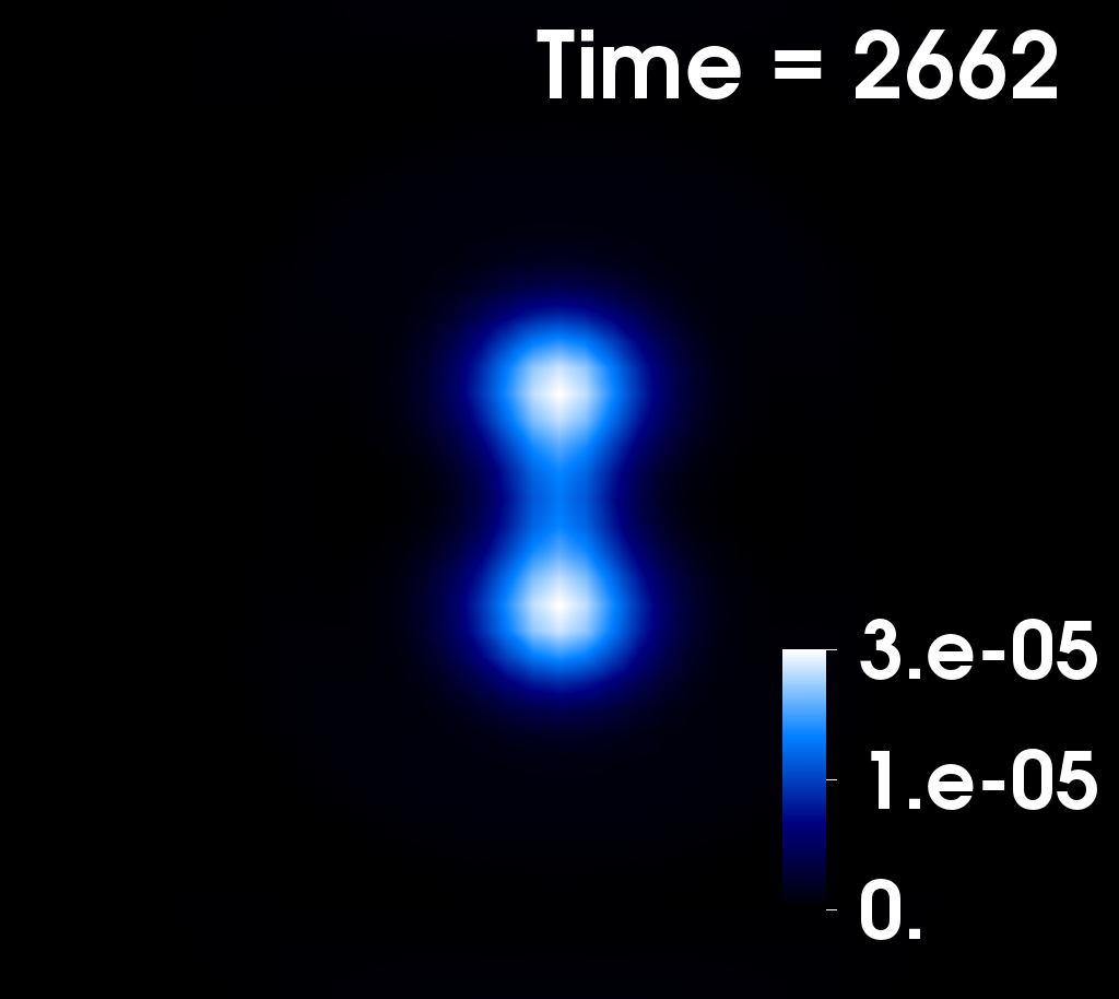
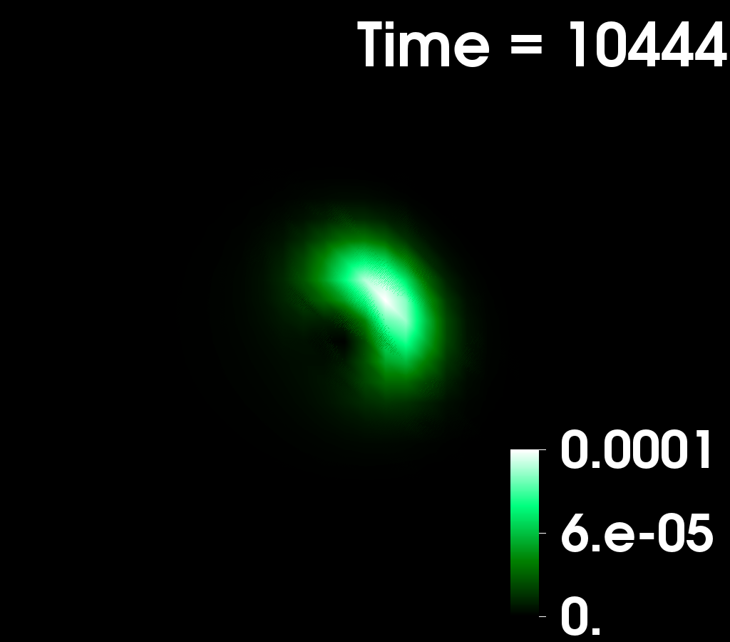
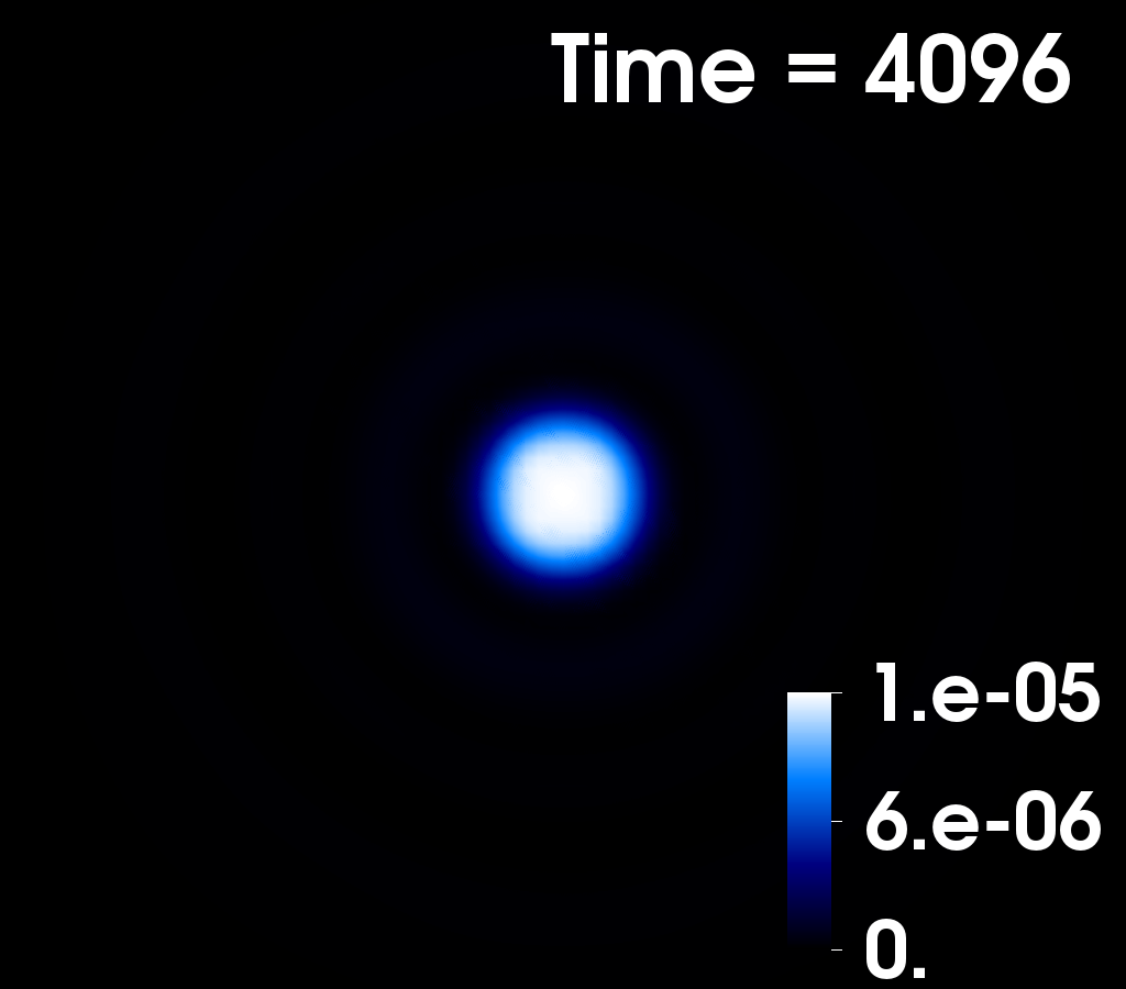
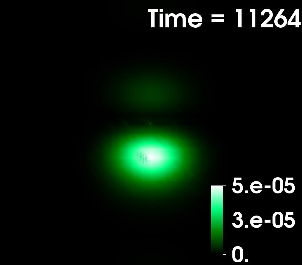
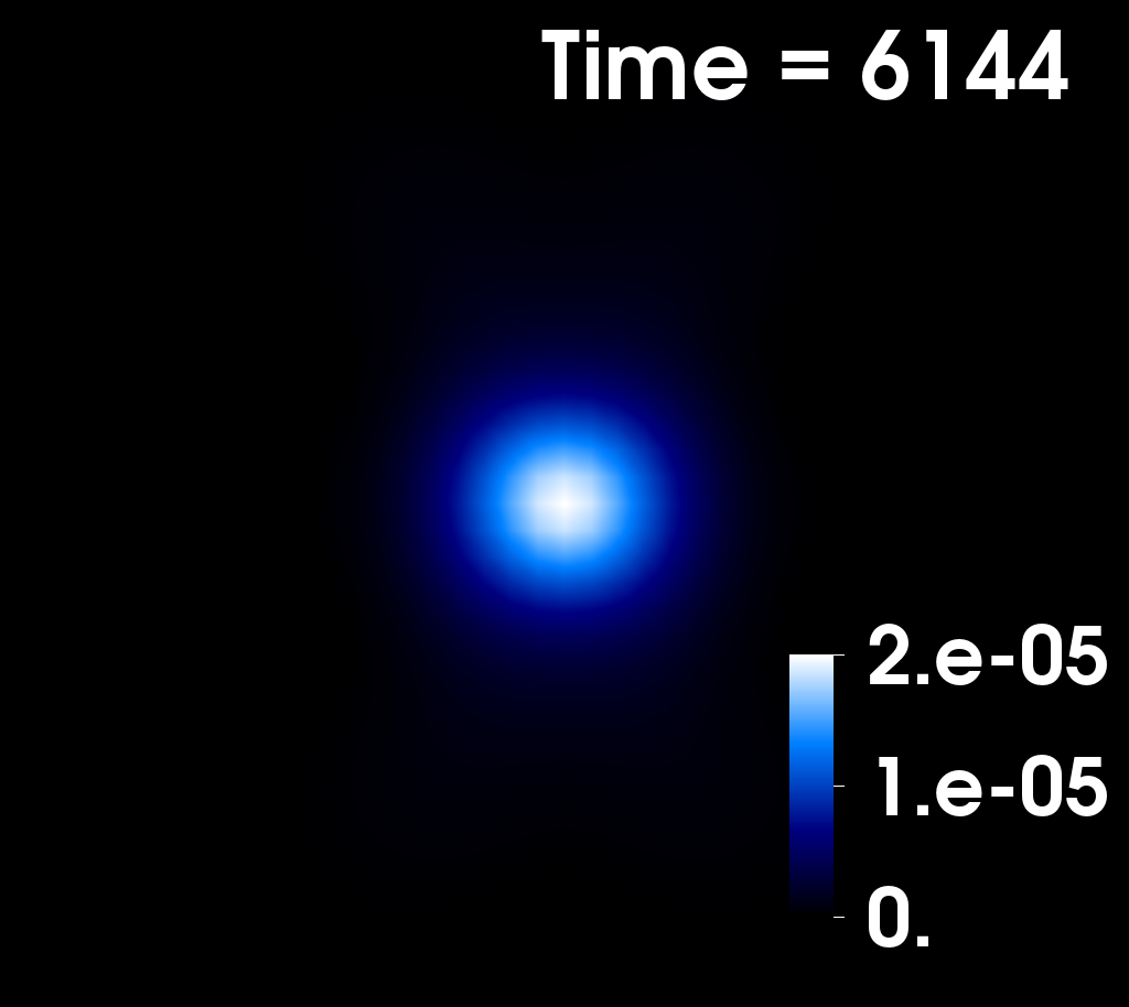
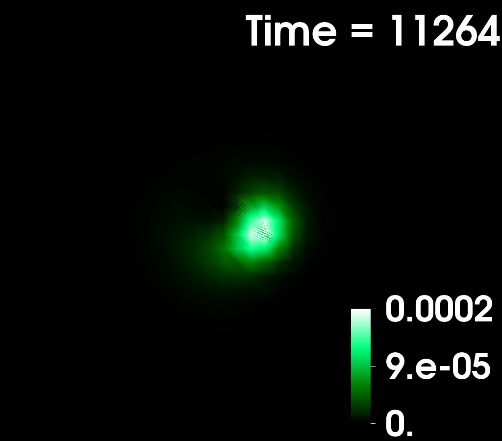
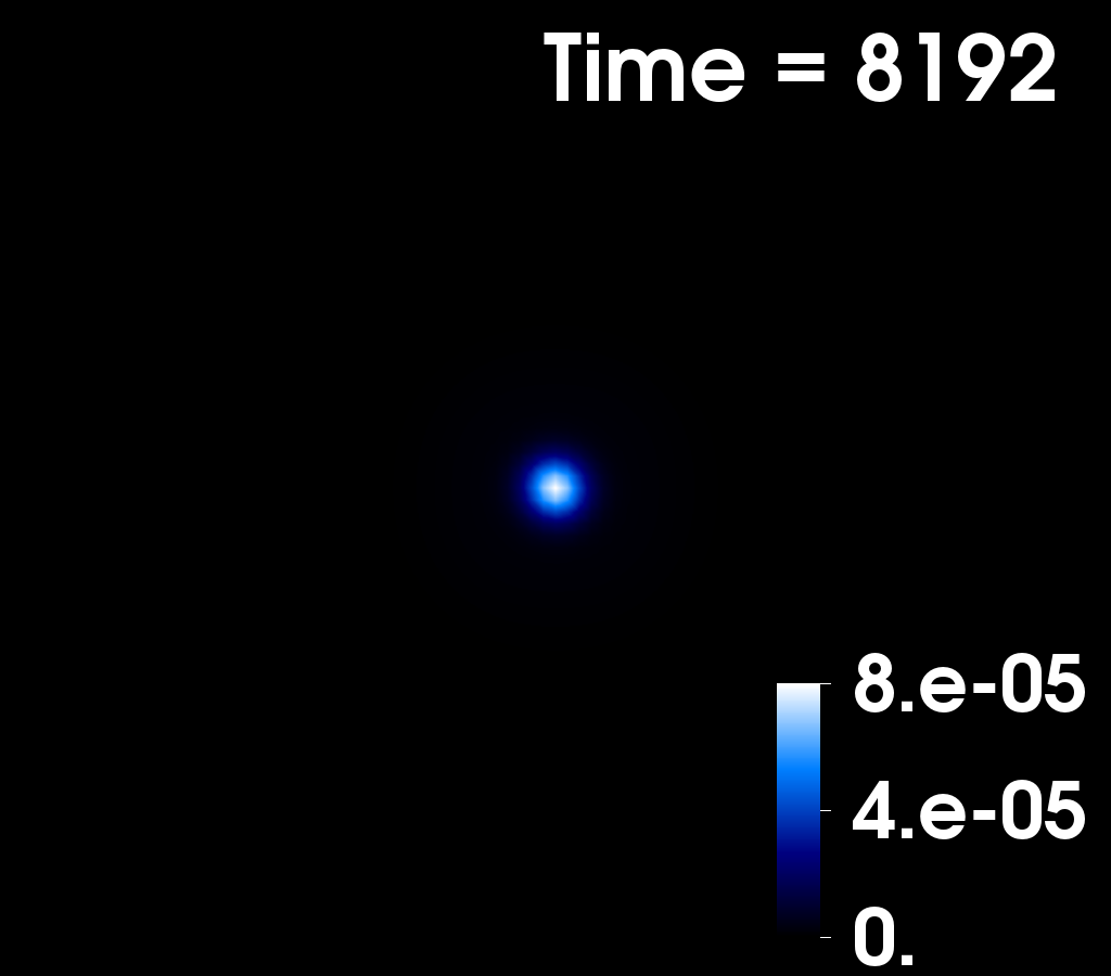
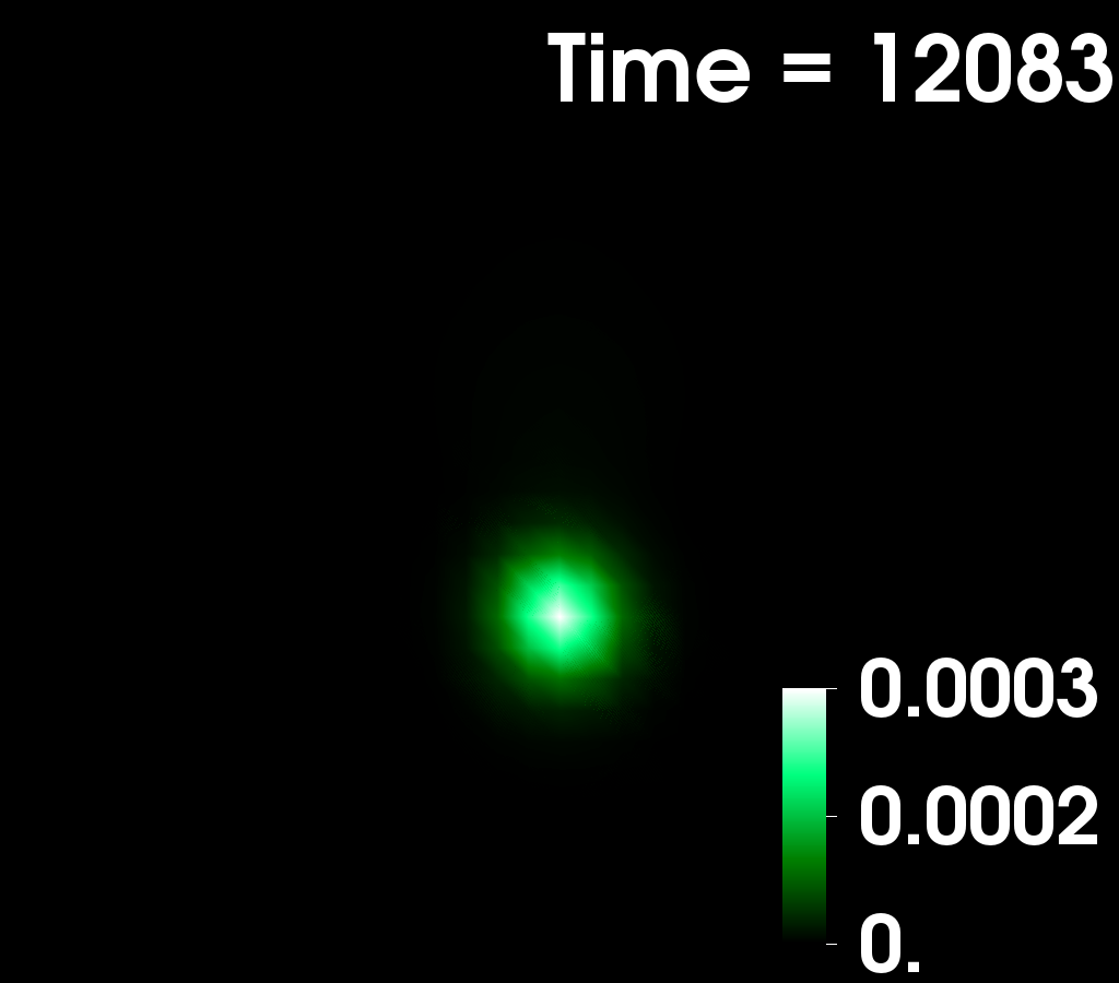
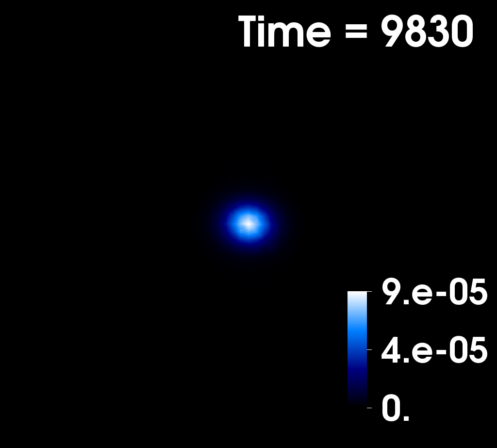
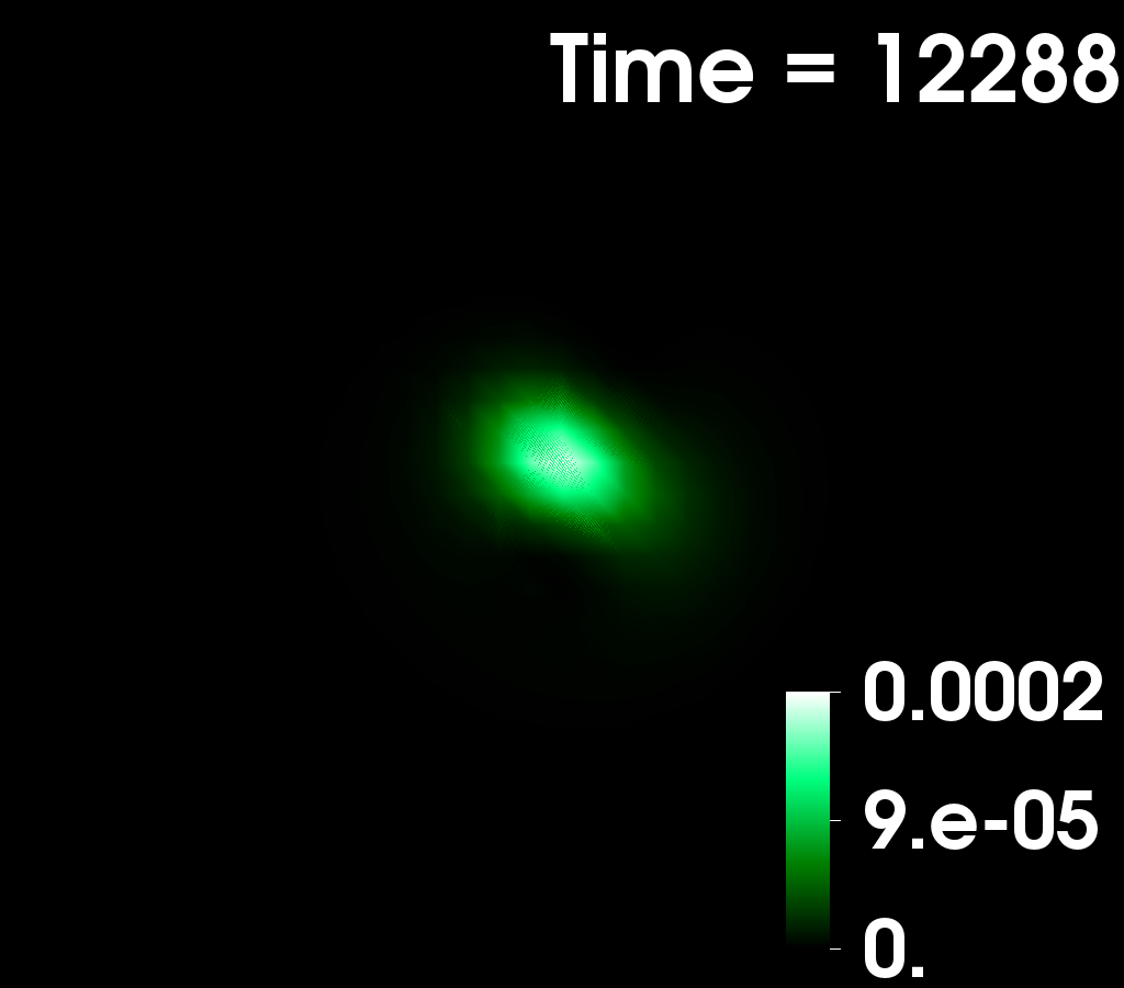
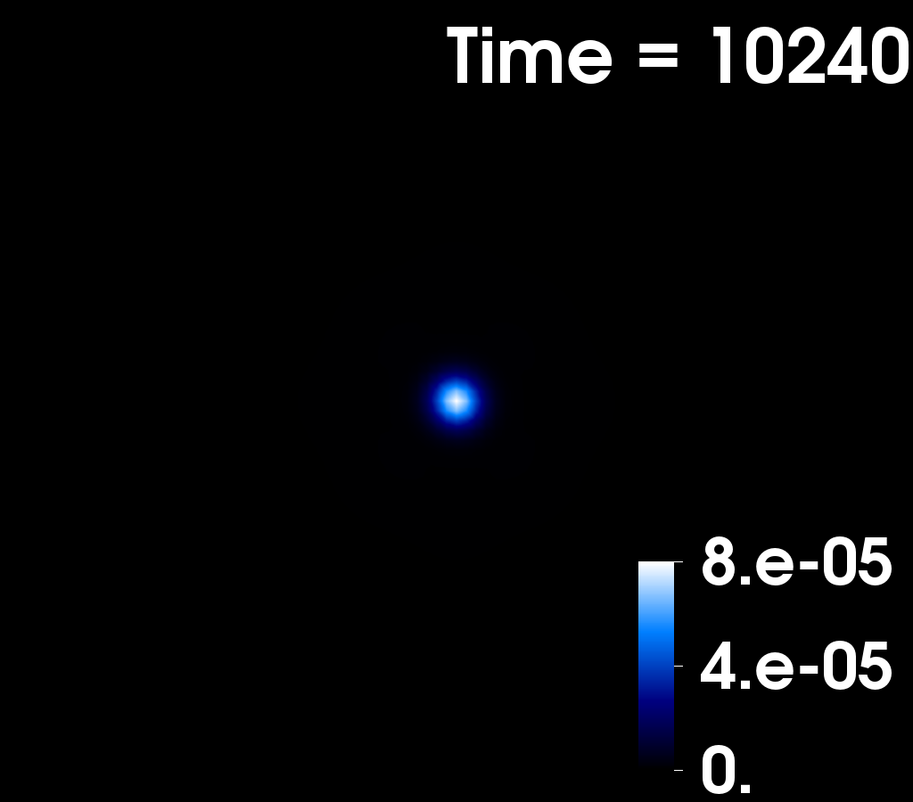
Figure 8: Time evolution (top to bottom) of the energy density (green for scalar/blue for vector) in the formation scenario of different BSs. The models in the first three columns become disrupted during the collapse. The model in the fourth column keeps its structure (it only becomes more compact) which shows that vector SBS₊₁+SBS_-1 are stable.

For instance, starting with dilute distributions of scalar field with the multipolar components of DBS₀, SBS_±1, and DBS₀+SBS₊₁, or of a vector field with the distribution of DBS₀, the collapse ends up disrupting the star; on the other hand, starting with dilute distributions of vector field with the multipolar components of SBS₊₁+SBS_-1, a compact object with these modes survives. The interested reader is addressed to Sanchis-Gual et al. (2019) for further details on the construction of constraint-solving initial data describing the cloud of bosonic matter that leads to the formation of SBS_±1.

The procedure we follow for the new configurations DBS₀ and for the multi-field BSs is the same, but with a different ansatz for the fields. In the case of scalar DBS₀ we consider the following

$$\Phi^{(0)}(t,r,\theta,\varphi)=Ae^{-\frac{r^{2}}{\sigma^{2}}}Y_{10}(\theta,\varphi)e^{-i\omega t},$$ (3)

where $Y_{10}(\theta,\varphi)=\cos{\theta}$ is the $\ell=1$, $m=0$ spherical harmonic, and $A$ and $\sigma$ are free parameters.

The formulation we adopt for the evolution of the Proca field is the one described in Zilhão et al. (2015) where the Proca field is split up into its scalar potential $\mathcal{X}_{\phi}$, its 3-vector potential $\mathcal{X}_{i}$ and the “electric” and “magnetic” fields $E^{i}$ and $B^{i}$. The vector case is more involved than the scalar one because one must solve also the Gauss constraint. Nevertheless, the procedure to solve the Gauss constraint for the vector DBS₀ is the same as the one we already used for vector SBS₁, which is described in Appendix A of Sanchis-Gual et al. (2019); one must make an ansatz for the scalar potential, which for DBS₀ is chosen as

$$\mathcal{X}_{\phi}(t,r,\theta,\varphi)=R(r)Y_{10}(\theta,\varphi)\,e^{-i\omega t}\,,$$ (4)

where $R(r)=r^{2}e^{-\frac{r^{2}}{\sigma^{2}}}$. Once the Gauss constraint is solved for the chosen scalar potential, we obtain the shape of all the other fields:

$$E^{r}(r,\theta)= \ \frac{A\,\sigma^{2}}{12r^{3}}\biggl{(}8\sigma^{4}-2e^{-\frac{r^{2}}{\sigma^{2}}}[3r^{4}+$$ (5)

$$\ 4r^{2}\sigma^{2}+4\sigma^{4}]-\sqrt{\pi}r^{3}\sigma\,\rm{Erf}\left(\frac{r}{\sigma}\right)\biggr{)}\cos{\theta}\ ,$$

$$E^{\theta}(r,\theta)= \ \frac{A\,\sigma e^{-\frac{r^{2}}{\sigma^{2}}}}{24r^{3}}\biggl{(}-e^{\frac{r^{2}}{\sigma^{2}}}\biggl{[}2\sqrt{\pi}\sigma^{2}r^{3}+8\sigma^{5}$$ (6)

$$-2\sqrt{\pi}\sigma^{3}r^{2}\,\rm{Erf}\left(\frac{r}{\sigma}\right)\biggr{]}+8r^{2}\sigma^{3}+8\sigma^{5}\biggr{)}\sin{\theta}\ ,$$

$$E^{\varphi}(r,\theta)= \ \frac{A\,\sigma e^{-\frac{r^{2}}{\sigma^{2}}}}{24r^{3}}\biggl{(}-e^{\frac{r^{2}}{\sigma^{2}}}\biggl{[}2\sqrt{\pi}\sigma^{2}r^{3}+8\sigma^{5}$$ (7)

$$-2\sqrt{\pi}\sigma^{3}r^{2}\,\rm{Erf}\left(\frac{r}{\sigma}\right)\biggr{]}+8r^{2}\sigma^{3}+8\sigma^{5}\biggr{)}\frac{\cos{\theta}}{\sin^{2}{\theta}}\ ,$$

$$\mathcal{X}_{i}(r,\theta)= \ \frac{1}{\alpha}(\omega+\beta^{\varphi})\gamma_{ij}E^{j}(r,\theta)\ .$$ (8)

As we are considering the case $m=0$ there is no dependence on the azimuthal coordinate $\varphi$ in the fields. Notice also that the radial dependence of the field is the same as for SBS₊₁, but its angular dependence is different.

References

- Abbott et al. (2016) B. P. Abbott, R. Abbott, T. D. Abbott, M. R. Abernathy, F. Acernese, K. Ackley, C. Adams, T. Adams, P. Addesso, R. X. Adhikari, and et al., Physical Review Letters 116, 061102 (2016), arXiv:1602.03837 [gr-qc] .
- Abbott et al. (2019) B. P. Abbott et al. (LIGO Scientific, Virgo), Phys. Rev. X 9, 031040 (2019), arXiv:1811.12907 [astro-ph.HE] .
- Abbott et al. (2020) R. Abbott et al. (LIGO Scientific, Virgo), (2020), arXiv:2010.14527 [gr-qc] .
- Akiyama et al. (2019) K. Akiyama et al. (Event Horizon Telescope), Astrophys. J. 875, L1 (2019).
- Gravity Collaboration et al. (2018) Gravity Collaboration, R. Abuter, A. Amorim, M. Bauböck, J. P. Berger, H. Bonnet, W. Brand ner, Y. Clénet, V. Coudé Du Foresto, and P. T. de Zeeuw, Astron. Astrophys. 618, L10 (2018), arXiv:1810.12641 [astro-ph.GA] .
- Calderón Bustillo et al. (2021) J. Calderón Bustillo, N. Sanchis-Gual, A. Torres-Forné, J. A. Font, A. Vajpeyi, R. Smith, C. Herdeiro, E. Radu, and S. H. W. Leong, Phys. Rev. Lett. 126, 081101 (2021), arXiv:2009.05376 [gr-qc] .
- Herdeiro et al. (2021a) C. A. R. Herdeiro, A. M. Pombo, E. Radu, P. V. P. Cunha, and N. Sanchis-Gual, (2021a), arXiv:2102.01703 [gr-qc] .
- Cardoso and Pani (2019) V. Cardoso and P. Pani, Living Rev. Rel. 22, 4 (2019), arXiv:1904.05363 [gr-qc] .
- Kaup (1968) D. J. Kaup, Phys. Rev. 172, 1331 (1968).
- Ruffini and Bonazzola (1969) R. Ruffini and S. Bonazzola, Phys. Rev. 187, 1767 (1969).
- Brito et al. (2016) R. Brito, V. Cardoso, C. A. R. Herdeiro, and E. Radu, Phys. Lett. B752, 291 (2016), arXiv:1508.05395 [gr-qc] .
- Liebling and Palenzuela (2012) S. L. Liebling and C. Palenzuela, Living Rev. Rel. 15, 6 (2012), arXiv:1202.5809 [gr-qc] .
- Note (1) In this paper we focus on non-self-interacting fields.
- Herdeiro et al. (2017) C. A. R. Herdeiro, A. M. Pombo, and E. Radu, Phys. Lett. B 773, 654 (2017), arXiv:1708.05674 [gr-qc] .
- Schunck and Mielke (1998) F. E. Schunck and E. W. Mielke, Phys. Lett. A249, 389 (1998).
- Yoshida and Eriguchi (1997) S. Yoshida and Y. Eriguchi, Phys. Rev. D56, 762 (1997).
- Herdeiro et al. (2019) C. Herdeiro, I. Perapechka, E. Radu, and Y. Shnir, Phys. Lett. B 797, 134845 (2019), arXiv:1906.05386 [gr-qc] .
- Herdeiro et al. (2021b) C. A. R. Herdeiro, J. Kunz, I. Perapechka, E. Radu, and Y. Shnir, Phys. Lett. B 812, 136027 (2021b), arXiv:2008.10608 [gr-qc] .
- Sanchis-Gual et al. (2019) N. Sanchis-Gual, F. Di Giovanni, M. Zilhão, C. Herdeiro, P. Cerdá-Durán, J. Font, and E. Radu, Physical Review Letters 123, 221101 (2019).
- Balakrishna et al. (1998) J. Balakrishna, E. Seidel, and W.-M. Suen, Phys. Rev. D58, 104004 (1998), arXiv:gr-qc/9712064 [gr-qc] .
- Bernal et al. (2010) A. Bernal, J. Barranco, D. Alic, and C. Palenzuela, Phys. Rev. D81, 044031 (2010), arXiv:0908.2435 [gr-qc] .
- Matos and Urena-Lopez (2007) T. Matos and L. A. Urena-Lopez, Gen. Rel. Grav. 39, 1279 (2007).
- Urena-Lopez and Bernal (2010) L. A. Urena-Lopez and A. Bernal, Phys. Rev. D 82, 123535 (2010), arXiv:1008.1231 [gr-qc] .
- Di Giovanni et al. (2020a) F. Di Giovanni, S. Fakhry, N. Sanchis-Gual, J. C. Degollado, and J. A. Font, Physical Review D 102, 084063 (2020a).
- Guzmán and Ureña López (2020) F. S. Guzmán and L. A. Ureña López, Phys. Rev. D 101, 081302 (2020), arXiv:1912.10585 [astro-ph.GA] .
- Guzmán (2021) F. S. Guzmán, Astronomische Nachrichten (2021).
- Alcubierre et al. (2018) M. Alcubierre, J. Barranco, A. Bernal, J. C. Degollado, A. Diez-Tejedor, M. Megevand, D. Nunez, and O. Sarbach, Class. Quant. Grav. 35, 19LT01 (2018), arXiv:1805.11488 [gr-qc] .
- Alcubierre et al. (2019) M. Alcubierre, J. Barranco, A. Bernal, J. C. Degollado, A. Diez-Tejedor, M. Megevand, D. Núñez, and O. Sarbach, Class. Quant. Grav. 36, 215013 (2019), arXiv:1906.08959 [gr-qc] .
- Jaramillo et al. (2020) V. Jaramillo, N. Sanchis-Gual, J. Barranco, A. Bernal, J. C. Degollado, C. Herdeiro, and D. Núñez, Phys. Rev. D 101, 124020 (2020), arXiv:2004.08459 [gr-qc] .
- Note (2) In spherical symmetry, multi-frequency BSs were discussed in Choptuik et al. (2019); and BSs in multi-scalar theories were recently constructed in Yazadjiev and Doneva (2019); Collodel et al. (2020).
- Smolić (2015) I. Smolić, Class. Quant. Grav. 32, 145010 (2015), arXiv:1501.04967 [gr-qc] .
- Note (3) For the -BS, moreover, the fields depend on both the Killing and coordinates but the total EMT does not, albeit the individual EMT of each scalar field may still depend on the coordinate.
- Note (4) The non-vanishing Einstein equations are , and . Four of them are solved together with the three Klein-Gordon eqs., yielding a coupled system of seven PDEs on the unknown functions . The remaining two Einstein equations are treated as constraints and used to check the numerical accuracy.
- Note (5) Excited solutions with exist as well.
- Herdeiro and Radu (2015) C. Herdeiro and E. Radu, Class. Quant. Grav. 32, 144001 (2015), arXiv:1501.04319 [gr-qc] .
- Note (6) It is in the notation of Herdeiro et al. (2021b).
- Herdeiro et al. (2021c) C. A. R. Herdeiro, J. Kunz, I. Perapechka, E. Radu, and Y. Shnir, (2021c), arXiv:2101.06442 [gr-qc] .
- Note (7) The same holds for the Noether charge of the fields.
- Note (8) Bare in mind each of these points is in fact a continuous family, spanning a range of frequencies.
- Note (9) Since is carried by even parity fields, the range is maximal (minimal) for (). This explains the triangular shape in Fig. 1.
- Note (10) The typical size of the BSs here is around 15-30; then means 400-800 light-crossing times.
- Note (11) See also Zeng et al. (2021) for another multi-state construction.
- Di Giovanni et al. (2020b) F. Di Giovanni, N. Sanchis-Gual, P. Cerdá-Durán, M. Zilhão, C. Herdeiro, J. A. Font, and E. Radu, Phys. Rev. D 102, 124009 (2020b), arXiv:2010.05845 [gr-qc] .
- Siemonsen and East (2021) N. Siemonsen and W. E. East, Phys. Rev. D 103, 044022 (2021), arXiv:2011.08247 [gr-qc] .
- Choptuik et al. (2019) M. Choptuik, R. Masachs, and B. Way, Phys. Rev. Lett. 123, 131101 (2019), arXiv:1904.02168 [gr-qc] .
- Yazadjiev and Doneva (2019) S. S. Yazadjiev and D. D. Doneva, Phys. Rev. D 99, 084011 (2019), arXiv:1901.06379 [gr-qc] .
- Collodel et al. (2020) L. G. Collodel, D. D. Doneva, and S. S. Yazadjiev, Phys. Rev. D 101, 044021 (2020), arXiv:1912.02498 [gr-qc] .
- Zeng et al. (2021) Y.-B. Zeng, H.-B. Li, S.-X. Sun, S.-Y. Cui, and Y.-Q. Wang, (2021), arXiv:2103.10717 [gr-qc] .
- Witek et al. (2020) H. Witek, M. Zilhao, G. Ficarra, and M. Elley, “Canuda: a public numerical relativity library to probe fundamental physics,” (2020).
- Zilhão et al. (2015) M. Zilhão, H. Witek, and V. Cardoso, Class. Quant. Grav. 32, 234003 (2015), arXiv:1505.00797 [gr-qc] .
- Seidel and Suen (1994) E. Seidel and W.-M. Suen, Phys. Rev. Lett. 72, 2516 (1994), arXiv:gr-qc/9309015 [gr-qc] .
- Di Giovanni et al. (2018) F. Di Giovanni, N. Sanchis-Gual, C. A. R. Herdeiro, and J. A. Font, Phys. Rev. D98, 064044 (2018), arXiv:1803.04802 [gr-qc] .