Anomaly Detection Algorithms for Location Security in 5G Scenarios

Abstract

Location based services are expected to play a major role in future generation cellular networks, starting from the incoming 5G systems. At the same time, localization technologies may be severely affected by attackers capable to deploy low cost fake base stations and use them to alter localization signals. In this paper, we concretely focus on two classes of threats: noise-like jammers, whose objective is to reduce the signal-to-noise ratio, and spoofing/meaconing attacks, whose objective is to inject false or erroneous information into the receiver. Then, we formulate the detection problems as binary hypothesis tests and solve them resorting to the generalized likelihood ratio test design procedure as well as the Latent Variable Models, which involves the expectation-maximization algorithm to estimate the unknown data distribution parameters. The proposed techniques can be applied to a large class of location data regardless the subsumed network architecture. The performance analysis is conducted over simulated data generated by using measurement models from the literature and highlights the effectiveness of the proposed approaches in detecting the aforementioned classes of attacks.

I Introduction

The incoming fifth generation mobile communication network (5G) will be capable of guaranteeing new reliable services, high data rates, low latency, and support for largely heterogeneous devices [1]. Localization services, which in the past were mainly provided by non-cellular technologies (e.g., Global Navigation Satelline Systems and/or Global Positioning Systems) integrated within the cellular devices, are now conceived as first class citizens of the 5G architecture starting from Release 16 [2, 3, 4], and will play a crucial role in several scenarios envisioned for 5G, including self-driving cars, unmanned aerial vehicles, smart logistics, emergency services, and many more [5, 6, 7]. At the same time, the ability to exploit location signals emitted by 5G base stations comes with a bleak side: many literature works [8, 9, 10, 11, 12, 13, 14, 15, 16, 17, 18, 19, 20] show how easy is for a tech savvy opponent to build ultra-low cost Jammers or even LTE/5G “rogue” base stations [21] capable to generate fake signals or interfere with legitimate ones. Moreover, since in 5G a large number of stages interact towards the position estimation, there exists a plethora of points of the distributed communication system that can be object of malicious actions. Therefore, it emerges the strong need to equip the 5G network with suitable countermeasures aimed at preserving location data integrity.

Among the possible threats to location security, here we focus on intentional interference, which involves hostile platforms that target the user equipment (UE) and/or Access Node (AN) receivers in order to [22, 23, 24, 25]: (i) reduce the signal-to-noise ratio (noise-like jamming); and (ii) inject false or erroneous information (spoofing/meaconing). (see also Figure 1, where the ANs are denoted by gNB)

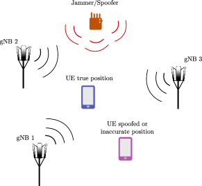
Figure 1: Operating scenario for a cellular network under the attack of a jammer or spoofer which leads to inaccurate or counterfeit location estimates.

The hostile platforms belonging to the first class of threats perform a denial of service attack by transmitting high-power interfering signals to disrupt the functionalities of the receiver and are referred to as noise-like jammers [26, 27, 25]. In fact, the signals transmitted by NLJs blend into the thermal noise of the receiver leading to an increase of the noise power spectral density within the receiver bandwidth and, hence, to a decrease of the signal-to-noise ratio (SNR). Remarkably, under the attack of NLJs, the estimation quality direction of arrival (DOA), time of arrival (TOA), time difference of arrival (TDOA), and received signal strength (RSS) measurements at a generic AN degrades and leads to inaccurate UE localization [28]. Most of the existing detection and mitigation strategies to cope with NLJ attacks in wireless networks take place at physical and/or protocol layer [29]. Anti-jamming techniques in the context of cognitive radio networks are addressed in [30], where several mitigation techniques are reviewed and a new anti-jamming protocol relying on probabilistic pairing and frequency tuning is proposed. Other examples of electronic counter-countermeasures are given in [31, 32] where an approach based on game theory is applied at the design stage. Mitigation solutions conceived at the physical layer can be found in [33], where the received signal is classified by means of a deep convolutional neural network fed by the signal features in the wavelet domain. Finally, in [34], the authors leverage random matrix theory tools to conceive a multiple hypothesis test for jamming detection. To this end, they estimate the jammer subspace through the sample covariance matrix [35] and project the received data onto the user subspace in order to mitigate the jamming components.

Platforms perpetrating the second mentioned class of attacks are aimed at deceiving the AN receiver by injecting fake information into the latter. These deceptive operations are commonly referred to as spoofing/meaconing [24, 22, 25] and intercept the positioning messages exchanged by two legitimate actors and suitably delay or modify them by synthesizing counterfeit information. Their main objective consists in preventing the victim systems from providing reliable position estimates. Deceptive attacks do not degrade the estimation quality of the location parameters but they are capable of changing the true parameter values. In the context of massive multiple-input multiple-output (MIMO) systems, a key feature of 5G networks, in [36], the generalized likelihood ratio test (GLRT) is applied to detect jamming signals contaminating user pilots. To this end, received raw data is first projected onto the subspace of the unused pilots in order to remove useful signal components and then the GLRT is derived by estimating the unknown parameters through the maximum likelihood approach. In [34], a pilot spoofing attack detection algorithm in massive MIMO systems is proposed, in which the information of channel statistics is unknown. First, users send pilots to the base station, then the latter transmits the conjugate of its received signal (which may contain spoofing signal) back to users, where the final detection is made.

Summarizing, the above contributions show that intentional interference detection/mitigation in wireless networks can be accomplished at different layers according to the desired trade-off between computational requirements and effectiveness. In fact, it is clear that processing raw data (physical layer) might lead to more reliable techniques at the price of an increased complexity, whereas algorithms fed by high-level data (namely, the measurements provided by the network sensors) might be more efficient. In addition, in the latter case, since a preliminary processing is performed on data, the available information is limited and, more importantly, affected by the uncertainties introduced by the early stages [37, 38, 39]. Nevertheless, in many situations raw data are not available given the specific architecture solutions and, hence, possible location security algorithms are limited to work with the measurements provided by the network infrastructure.

It is important to stress here that the New Radio (NR)-positioning work started with release 16 and [2] presents the agreed positioning techniques, including the main signal and measurements considered at the UE and gNB side (i.e., downlink and uplink TDOA, angle-of-arrival (AOA), reference signal received power (RSRP)). More importantly, further standardization work is ongoing for enhanced localization services. Therefore, in this paper, we present a class of approaches for the detection of anomalies due to intentional interference that aim at being general enough to be adapted to the current studied techniques and possible future techniques of the 5G NR as well as different types of location data (e.g., TDOA and AOA).

We first formulate the detection problem at hand in terms of a binary hypothesis test where data under the null hypothesis are homogeneous and distinguishing between either NLJ or spoofing/meaconing attacks. At the design stage, we assume two statistical models for the available measurements that differ in the level of correlation among them. In order to solve the hypothesis test, we resort to both the plain GLRT and to an ad hoc modification that incorporates the latent variable model (LVM) [40] (a point better explained in Section III and IV). The performance analysis is conducted over both simulated and highlights the effectiveness of the proposed approach. Finally, it is important to underline that such architectures can be thought as a component of the location enablers of 5G that performs a preliminary analysis of data and provides a possible alert about the presence of an attack. This alert is then jointly exploited by the mitigation and localization function to remedy possible information counterfeit.

The remainder of the paper is organized as follows. Section II is devoted to sensor model description and to the formalization of the detection problems at hand, while the designs of the detection architectures are described in Section III and IV for NLJ and spoofing attacks, respectively. In Section V, some illustrative examples are provided to show the effectiveness of the proposed strategies. Finally, Section VI contains concluding remarks and charts a course for future works.

I-A Notation

In the sequel, vectors and matrices are denoted by boldface lower-case and upper-case letters, respectively. Symbols $\det(\cdot)$, $\mbox{\rm Tr}\,(\cdot)$, and $(\cdot)^{T}$ denote the determinant, trace, and transpose, respectively. As to the numerical sets, ${\mathds{R}}$ is the set of real numbers and ${\mathds{R}}^{N\times M}$ is the Euclidean space of $(N\times M)$-dimensional real matrices (or vectors if $M=1$). The Euclidean norm of a generic vector $\bm{x}$ is denoted by $\|\bm{x}\|$ whereas the modulus of a real number $x$ is denoted by $|x|$. For any $N$-dimensional vector $\bm{x}$, $\bm{X}=\mbox{\rm\bf diag}\,\{\bm{x}\}$ is a $(N\times N)$-dimensional diagonal matrix whose principal diagonal contains the elements of $\bm{x}$. Symbols $\bm{I}$ and $\bm{0}$ indicate the identity matrix and the null matrix or vector, respectively, whose size depends on the context. The curled inequality symbol $\succeq$ (and its strict form $\succ$) is used to denote generalized matrix inequality: for any $N$-dimensional Hermitian matrix $\bm{A}$, $\bm{A}\succeq\bm{0}$ means that $\bm{A}$ is a positive semi-definite matrix ($\bm{A}\succ\bm{0}$ for positive definiteness). Finally, we write $\bm{x}\sim\mbox{$\mathcal{N}$}_{N}(\bm{m},\bm{M})$ if $\bm{x}$ is a $N$-dimensional Gaussian vector with mean $\bm{m}$ and covariance matrix $\bm{M}\succ\bm{0}$, whereas, given $\bm{X}\in{\mathds{R}}^{N\times K}$, $\bm{X}\sim\mbox{$\mathcal{N}$}_{N}(\bm{m},\bm{M},\bm{I})$ means that the columns of $\bm{X}$ are Independent and Identically Distributed (IID) random vectors following the Gaussian distribution with mean $\bm{m}$ and covariance matrix $\bm{M}$.

II Sensor Model and Problem Formulation

Consider a slowly moving UE that is under tracking by the network infrastructure. Let us denote by $\bm{Z}=[\bm{z}_{1},\bm{z}_{2},\ldots,\bm{z}_{K}]\in{\mathds{R}}^{N\times K}$ the entire data matrix whose $k$th column, $k=1,\ldots,K$, contains a set of measurements acquired at the $k$th time istant. For instance, such measurements can be DOA, the TOA, the observed time difference of arrival (OTDOA), the RSRP, or others provided by the network.

In what follows, we assume that the measurement errors are independent over the time and thdic

the Gaussian distribution with zero mean and covariance matrix depending upon the specific operating scenario (a point better explained below). Thus, in a scenario unaffected by malicious platform actions, all the measurement are IID, namely

$$\bm{z}_{k}\sim\mbox{$\mathcal{N}$}_{N}(\bm{m},\bm{\varSigma}),\quad k=1,\ldots,K,$$ (1)

where $\bm{m}\in{\mathds{R}}^{N\times 1}$ contains the actual values of the considered location parameters and $\bm{\Sigma}\in{\mathds{R}}^{N\times N}$ is the positive definite error covariance matrix, which either can exhibit a generic symmetric structure or can be diagonal. The former case allows to accounts for a possible correlation among the measurements at the design stage, whereas the latter case corresponds to independent measurements.

Now, if at a certain time index, $K_{0}$ say, within the observation interval, a malicious platform performs an attack aimed at disrupting the receiver functionalities by transmitting noise-like signals, the quality of the estimates provided by the sensors would impair due to an increased uncertainty. As a consequence, data matrix can be partitioned into the following two submatrices $\bm{Z}_{1:K_{0}}\sim\mbox{$\mathcal{N}$}_{N}(\bm{m},\bm{\Sigma}_{1},\bm{I})$ and $\bm{Z}_{K_{0}+1:K}\sim\mbox{$\mathcal{N}$}_{N}(\bm{m},\bm{\Sigma}_{2},\bm{I})$, where $\bm{Z}_{1:K_{0}}=[\bm{z}_{1},\ldots,\bm{z}_{K_{0}}]\in{\mathds{R}}^{N\times K_{0}}$, $\bm{Z}_{K_{0}+1:K}=[\bm{z}_{K_{0}+1},\ldots,\bm{z}_{K}]\in{\mathds{R}}^{N\times(K-K_{0})}$, $\bm{\Sigma}_{2}-\bm{\Sigma}_{1}\succ\bm{0}$, and $K_{0}\in\Omega_{0}\subseteq\Omega=\{1,\ldots,K\}$. Under the above assumptions, the detection problem at hand can be formulated in terms of the following hypothesis test

$$\left\{\begin{aligned} &H_{0}:\bm{Z}\sim\mbox{$\mathcal{N}$}_{N}(\bm{m}_{0},\bm{\Sigma}_{0},\bm{I}),\\ &H_{1}:\begin{cases}\bm{Z}_{1:K_{0}}\sim\mbox{$\mathcal{N}$}_{N}(\bm{m}_{1},\bm{\Sigma}_{1},\bm{I}),\\ \bm{Z}_{K_{0}+1:K}\sim\mbox{$\mathcal{N}$}_{N}(\bm{m}_{1},\bm{\Sigma}_{2},\bm{I}),\end{cases}\end{aligned}\right.$$ (2)

where $\bm{m}$, $\bm{\Sigma}_{0}\succ\bm{0}$, $\bm{\Sigma}_{1}\succ\bm{0}$, $\bm{\Sigma}_{2}\succ\bm{0}$, and $K_{0}$ are unknown.

On the other hand, if the hostile platform is aimed at injecting false information into the network receivers, then, starting from the time instant $K_{0}$, the mean vector no longer contains the true position of the UE but its entries are related to the false position information created by the attacker. Therefore, in this case, the considered detection problem becomes

$$\left\{\begin{aligned} &H_{0}:\bm{Z}\sim\mbox{$\mathcal{N}$}_{N}(\bm{m}_{0},\bm{\Sigma}_{0},\bm{I}),\\ &H_{1}:\begin{cases}\bm{Z}_{1:K_{0}}\sim\mbox{$\mathcal{N}$}_{N}(\bm{m}_{1},\bm{\Sigma}_{1},\bm{I}),\\ \bm{Z}_{K_{0}+1:K}\sim\mbox{$\mathcal{N}$}_{N}(\bm{m}_{2},\bm{\Sigma}_{1},\bm{I}),\end{cases}\end{aligned}\right.$$ (3)

where $\bm{m}_{1}\in{\mathds{R}}^{N\times 1}$ is an unknown vector containing the location information before that spoofing takes place, $\bm{m}_{2}\in{\mathds{R}}^{N\times 1}$ is an unknown vector representing the modified position due to the attack, $\bm{\Sigma}_{1}\succ\bm{0}$, and, again, $K_{0}$ is unknown.

In the next section, we devise different detection architectures for the above problems relying on the GLRT and LVM.

Before concluding this section, we provide some definitions which come in handy for the next developments. More precisely, the probability density function (PDF) of $\bm{Z}$ under $H_{0}$ for both problems has the following expression $f_{0}(\bm{Z};\bm{m}_{0},\!\bm{\Sigma}_{0})\!\!\!\!\!=\!\!\!\!\!\prod_{k=1}^{K}\!f_{0}(\bm{z}_{k};\bm{m}_{0},\!\bm{\Sigma}_{0})$, while the PDFs of $\bm{Z}$ under $H_{1}$ for problems (2) and (3) are given by $f_{1}(\bm{Z};\bm{m}_{1},\bm{\Sigma}_{1},\bm{\Sigma}_{2},K_{0})=\prod_{k=1}^{K_{0}}f_{1}(\bm{z}_{k};\bm{m}_{1},\bm{\Sigma}_{1})$ $\times\prod_{k=K_{0}+1}^{K}f_{1}(\bm{z}_{k};\bm{m}_{1},\bm{\Sigma}_{2})$ and $f_{1}(\bm{Z};\bm{m}_{1},\bm{m}_{2},\bm{\Sigma}_{1},K_{0})=\prod_{k=1}^{K_{0}}\!f_{1}(\bm{z}_{k};\bm{m}_{1},\!\bm{\Sigma}_{1})\!\prod_{k=K_{0}+1}^{K}\!f_{1}(\bm{z}_{k};\bm{m}_{2},\!\bm{\Sigma}_{1})$, respectively, where

$$f_{l}(\bm{z}_{k};\bm{m}_{m},\bm{\Sigma}_{n})\\ =\frac{\exp\left\{\displaystyle-\frac{1}{2}\mbox{\rm Tr}\,[\bm{\Sigma}_{n}^{-1}(\bm{z}_{k}-\bm{m}_{m})(\bm{z}_{k}-\bm{m}_{m})^{T}]\right\}}{(2\pi)^{N/2}[\det(\bm{\Sigma}_{n})]^{1/2}}$$ (4)

with $l=0,1$, $m=0,1,2$, and $n=0,1,2$.

III Noise-like Jammer Detectors

Decision rules presented in this section are derived under the design assumptions of problem (2) assuming different structures for the error covariance matrices. Moreover, for the most general covariance structure, start with the plain GLRT whose general structure is given by

$$\frac{\displaystyle\max_{K_{0}\in\Omega_{0}}\displaystyle\max_{\bm{m}_{1}}\displaystyle\max_{\bm{\Sigma}_{1}}\displaystyle\max_{\bm{\Sigma}_{2}}f_{1}(\bm{Z};\bm{m}_{1},\bm{\Sigma}_{1},\bm{\Sigma}_{2},K_{0})}{\displaystyle\max_{\bm{m}_{0}}\displaystyle\max_{\bm{\Sigma}_{0}}f_{0}(\bm{Z};\bm{m}_{0},\bm{\Sigma}_{0})}\mbox{$\begin{array}[]{c}\stackrel{{\scriptstyle\stackrel{{\scriptstyle\textstyle H_{1}}}{{\textstyle>}}}}{{\stackrel{{\scriptstyle\textstyle<}}{{\textstyle H_{0}}}}}\end{array}$}\eta,$$ (5)

where $\Omega_{0}\subseteq\{1,\ldots,K\}$ and $\eta$ is the detection threshold to be set in order to ensure a preassigned Probability of False Alarm ($P_{\text{fa}}$), and consider two cases

• the available measurements are uncorrelated leading to diagonal covariance matrices;

• there exists a correlation among the measurements, i.e., the covariance matrices are generally symmetric.

III-A GLRT for Uncorrelated Measurements

In this case, we assume that $\bm{\Sigma}_{0}=\mbox{\rm\bf diag}\,\{\sigma^{2}_{0,1},\ldots,\sigma^{2}_{0,N}\}$, $\bm{\Sigma}_{1}=\mbox{\rm\bf diag}\,\{\sigma^{2}_{1,1},\ldots,\sigma^{2}_{1,N}\}$, and $\bm{\Sigma}_{2}=\mbox{\rm\bf diag}\,\{\sigma^{2}_{2,1},\ldots,\sigma^{2}_{2,N}\}$ $=\mbox{\rm\bf diag}\,\{\sigma^{2}_{1,1}+\Delta\sigma^{2}_{1},\ldots,\sigma^{2}_{1,N}+\Delta\sigma^{2}_{N}\}$. Now, in order to compute the left-hand side of (5), we begin with the optimization problems under $H_{0}$. To this end, for computational convenience, we consider the log-likelihood function that, neglecting the constants irrelevant to the maximization, can be written as

$$\mbox{$\mathcal{L}$}_{0}(\bm{m}_{0},\bm{\Sigma}_{0};\bm{Z})\approx-\frac{K}{2}\sum_{n=1}^{N}\log{\sigma_{0,n}^{2}}\\ -\frac{1}{2}\sum_{k=1}^{K}\sum_{n=1}^{N}\frac{(z_{k,n}-m_{0,n})^{2}}{\sigma_{0,n}^{2}},$$ (6)

$m_{0,1},\ldots,m_{0,N}$ are the entries of $\bm{m}_{0}$ and $z_{k,1},\ldots,z_{k,N}$ are the entries of $\bm{z}_{k}$, $k=1,\ldots,K$. Setting to zero the gradient of $\mbox{$\mathcal{L}$}_{0}(\bm{m}_{0},\bm{\Sigma}_{0};\bm{Z})$ with respect to $\bm{m}_{0}$ and $\bm{\Sigma}_{0}$, we come up with the following estimates for $n=1,\ldots,N$

$$\widehat{m}_{0,n}=\frac{1}{K}\sum_{k=1}^{K}z_{k,n},\qquad\displaystyle\widehat{\sigma}^{2}_{0,n}=\frac{1}{K}\sum_{k=1}^{K}(z_{k,n}-\widehat{m}_{0,n})^{2},$$ (7)

which are maximum points since, $\forall n=1,\ldots,N$, the following inequalities hold

$$\begin{cases}\forall{\sigma}^{2}_{0,n}\!\!<\!\!\displaystyle\frac{1}{K}\sum_{k=1}^{K}(z_{k,n}-{m}_{0,n})^{2}:&\!\!\!\!\!\!\!\displaystyle\frac{\partial}{\partial\sigma^{2}_{0,n}}[\mbox{$\mathcal{L}$}_{0}(\bm{m}_{0},\bm{\Sigma}_{0};\bm{Z})]>0,\\ \forall{\sigma}^{2}_{0,n}\!\!>\!\!\displaystyle\frac{1}{K}\sum_{k=1}^{K}(z_{k,n}-{m}_{0,n})^{2}:&\!\!\!\!\!\!\!\displaystyle\frac{\partial}{\partial\sigma^{2}_{0,n}}[\mbox{$\mathcal{L}$}_{0}(\bm{m}_{0},\bm{\Sigma}_{0};\bm{Z})]<0,\\ \displaystyle\forall{m}_{0,n}\!\!<\!\!\frac{1}{K}\sum_{k=1}^{K}z_{k,n}:&\!\!\!\!\!\!\!\displaystyle\frac{\partial}{\partial m_{0,n}}[\mbox{$\mathcal{L}$}_{0}(\bm{m}_{0},\bm{\Sigma}_{0};\bm{Z})]>0,\\ \displaystyle\forall{m}_{0,n}\!\!>\!\!\frac{1}{K}\sum_{k=1}^{K}z_{k,n}:&\!\!\!\!\!\!\!\displaystyle\frac{\partial}{\partial m_{0,n}}[\mbox{$\mathcal{L}$}_{0}(\bm{m}_{0},\bm{\Sigma}_{0};\bm{Z})]<0.\end{cases}$$ (8)

As for the maximization under $H_{1}$, the corresponding log-likelihood function can be written (again neglecting the irrelevant constants) as follows

$$\mbox{$\mathcal{L}$}_{1}(\bm{m}_{1},\bm{\Sigma}_{1},\bm{\Sigma}_{2},K_{0};\bm{Z})\approx-\frac{K_{0}}{2}\sum_{n=1}^{N}\log\sigma_{1,n}^{2}\\ -\frac{K_{1}}{2}\sum_{n=1}^{N}\log(\sigma_{1,n}^{2}+\Delta\sigma_{n}^{2})-\frac{1}{2}\sum_{k=1}^{K_{0}}\sum_{n=1}^{N}\frac{(z_{k,n}-{m}_{1,n})^{2}}{\sigma_{1,n}^{2}}\\ -\frac{1}{2}\sum_{k=K_{0}+1}^{K}\sum_{n=1}^{N}\frac{({z}_{k,n}-{m}_{1,n})^{2}}{\sigma^{2}_{1,n}+\Delta\sigma^{2}_{n}},$$ (9)

where $K_{1}=K-K_{0}$. Before proceeding with the search of the stationary points of $\mbox{$\mathcal{L}$}_{1}(\bm{m}_{1},\bm{\Sigma}_{1},\bm{\Sigma}_{2},K_{0};\bm{Z})$, we compute the following limits that tell us where the stationary points can be sought, namely

$$\lim_{\|\bm{m}\|\rightarrow+\infty}\mbox{$\mathcal{L}$}_{1}(\bm{m}_{1},\bm{\Sigma}_{1},\bm{\Sigma}_{2},K_{0};\bm{Z})=-\infty,$$

$$\lim_{\sigma_{1,n}^{2}\rightarrow+\infty}\mbox{$\mathcal{L}$}_{1}(\bm{m}_{1},\bm{\Sigma}_{1},\bm{\Sigma}_{2},K_{0};\bm{Z})=-\infty,\ n=1,\ldots,N,$$

$$\lim_{\sigma_{1,n}^{2}\rightarrow 0}\mbox{$\mathcal{L}$}_{1}(\bm{m}_{1},\bm{\Sigma}_{1},\bm{\Sigma}_{2},K_{0};\bm{Z})=-\infty,\ n=1,\ldots,N,$$

$$\lim_{\Delta\sigma_{n}^{2}\rightarrow+\infty}\mbox{$\mathcal{L}$}_{1}(\bm{m}_{1},\bm{\Sigma}_{1},\bm{\Sigma}_{2},K_{0};\bm{Z})=-\infty,\ n=1,\ldots,N,$$

$$\lim_{\Delta\sigma_{n}^{2}\rightarrow 0}\mbox{$\mathcal{L}$}_{1}(\bm{m}_{1},\bm{\Sigma}_{1},\bm{\Sigma}_{2},K_{0};\bm{Z})=C\in{\mathds{R}},\ n=1,\ldots,N.$$

Thus, we can search the stationary points in the interior of the log-likelihood domain by setting to zero the first derivatives with respect to the unknown parameters. As first step, we consider the maximization with respect to $\sigma^{2}_{1,n}$ and $\Delta\sigma^{2}_{1,n}$, $n=1,\ldots,N$. To this end, let us compute

$$\frac{\partial}{\partial\Delta\sigma^{2}_{1,n}}[\mbox{$\mathcal{L}$}_{1}(\bm{m}_{1},\bm{\Sigma}_{1},\bm{\Sigma}_{2},K_{0};\bm{Z})]=0,\ n=1,\ldots,N,$$ (10)

which leads to the following equality for $n=1,\ldots,N$

$$\widehat{\Delta\sigma^{2}_{n}}(\sigma_{1,n}^{2},m_{1,n})=\begin{cases}\displaystyle\frac{1}{K_{1}}\sum_{k=K_{0}+1}^{K}(z_{k,n}-m_{1,n})^{2}-\sigma_{1,n}^{2}\\ \mbox{ if }\widehat{\Delta\sigma^{2}_{n}}>0,\\ 0,\mbox{ otherwise}.\end{cases}$$ (11)

Now, let $\Gamma_{N}=\{1,\ldots,N\}$ and, given a value of $K_{0}$, define the following sets

$$\Gamma(K_{0}) =\{n\in\Gamma_{N}:\ \widehat{\Delta\sigma^{2}_{n}}(\sigma_{1,n}^{2},m_{1,n})>0\}\subseteq\Gamma_{N},$$ (12)

$$\bar{\Gamma}(K_{0}) =\{n\in\Gamma_{N}:\ \widehat{\Delta\sigma^{2}_{n}}(\sigma_{1,n}^{2},m_{1,n})=0\}\subseteq\Gamma_{N}.$$ (13)

Thus, replacing the above stationary points in (9) and exploiting the last two definitions, we obtain (neglecting the constants) a

$$\mbox{$\mathcal{L}$}_{1}(\bm{m}_{1},\bm{\Sigma}_{1},\widehat{\bm{\Sigma}}_{2},K_{0};\bm{Z})\approx-\frac{K_{0}}{2}\sum_{n=1}^{N}\log\sigma_{1,n}^{2}\\ -\frac{K_{1}}{2}\sum_{n\in\Gamma(K_{0})}\log\left[\frac{1}{K_{1}}\sum_{k=K_{0}+1}^{K}(z_{k,n}-m_{1,n})^{2}\right]\\ -\frac{K_{1}}{2}\sum_{n\in\bar{\Gamma}(K_{0})}\log\sigma_{1,n}^{2}-\frac{1}{2}\sum_{n=1}^{N}\sum_{k=1}^{K_{0}}\frac{(z_{k,n}-{m}_{1,n})^{2}}{\sigma_{1,n}^{2}}\\ -\frac{1}{2}\sum_{n\in\bar{\Gamma}(K_{0})}\sum_{k=K_{0}+1}^{K}\frac{(z_{k,n}-{m}_{1,n})^{2}}{\sigma_{1,n}^{2}}.$$ (14)

Let us proceed by setting to zero the first derivative of $\mbox{$\mathcal{L}$}_{1}(\bm{m}_{1},\bm{\Sigma}_{1},\widehat{\bm{\Sigma}}_{2},K_{0};\bm{Z})$ with respect to $\sigma_{1,n}$, $n\in\Gamma(K_{0})\cup\bar{\Gamma}(K_{0})$, to obtain

$$\widehat{\sigma}_{1,n}^{2}(m_{1,n}) =\frac{1}{K_{0}}\sum_{k=1}^{K_{0}}(z_{k,n}-m_{1,n})^{2},\ n\in\Gamma(K_{0}),$$

$$\widehat{\sigma}_{1,n}^{2}(m_{1,n}) =\frac{1}{K}\sum_{k=1}^{K}(z_{k,n}-m_{1,n})^{2},\ n\in\bar{\Gamma}(K_{0}).$$ (15)

It follows that the compressed log-likelihood function can be written as

$$\mbox{$\mathcal{L}$}_{1}(\bm{m}_{1},\widehat{\bm{\Sigma}}_{1},\widehat{\bm{\Sigma}}_{2},K_{0};\bm{Z})\\ \approx-\frac{K_{0}}{2}\sum_{n\in\Gamma(K_{0})}\log\left[\frac{1}{K_{0}}\sum_{k=1}^{K_{0}}(z_{k,n}-m_{1,n})^{2}\right]\\ -\frac{K_{1}}{2}\sum_{n\in\Gamma(K_{0})}\log\left[\frac{1}{K_{1}}\sum_{k=K_{0}+1}^{K}(z_{k,n}-m_{1,n})^{2}\right]\\ -\frac{K}{2}\sum_{n\in\bar{\Gamma}(K_{0})}\log\left[\frac{1}{K}\sum_{k=1}^{K}(z_{k,n}-m_{1,n})^{2}\right].$$ (16)

It still remains to maximize the log-likelihood function with respect to $\bm{m}_{1}$ and $K_{0}$. To this end, we observe that optimization over $K_{0}$ can be carried out through a $1$-dimensional grid search, whereas an estimate of $\bm{m}_{1}$ can be obtained by solving the following system of equations

$$\frac{\partial}{\partial m_{1,n}}[\mbox{$\mathcal{L}$}_{1}(\bm{m}_{1},\widehat{\bm{\Sigma}}_{1},\widehat{\bm{\Sigma}}_{2},K_{0};\bm{Z})]=0,\ n\in\Gamma(K_{0})\cup\bar{\Gamma}(K_{0}).$$ (17)

When $n\in\bar{\Gamma}(K_{0})$, it is not difficult to show that the corresponding equation leads to $\widehat{m}_{0,n}$ given by (7), whereas in the case where $n\in{\Gamma}(K_{0})$, we have to solve

$$\frac{\displaystyle\sum_{k=1}^{K_{0}}z_{k,n}-K_{0}m_{1,n}}{\displaystyle\frac{1}{K_{0}}\sum_{k=1}^{K_{0}}(z_{k,n}-m_{1,n})^{2}}+\frac{\displaystyle\sum_{k=K_{0}+1}^{K}z_{k,n}-K_{1}m_{1,n}}{\displaystyle\frac{1}{K_{1}}\sum_{k=K_{0}+1}^{K}(z_{k,n}-m_{1,n})^{2}}=0$$

$$\Rightarrow\frac{1}{K_{1}}\sum_{k=K_{0}+1}^{K}(z_{k,n}-m_{1,n})^{2}\left[\sum_{k=1}^{K_{0}}z_{k,n}-K_{0}m_{1,n}\right]$$

$$+\frac{1}{K_{0}}\sum_{k=1}^{K_{0}}(z_{k,n}-m_{1,n})^{2}\left[\sum_{k=K_{0}+1}^{K}z_{k,n}-K_{1}m_{1,n}\right]=0.$$ (18)

Now, let us define the following quantities $A_{K_{0},n}=\sum_{k=1}^{K_{0}}z_{k,n}$, $\quad B_{K_{0},n}=\sum_{k=1}^{K_{0}}z_{k,n}^{2}$, $A_{K_{1},n}=\sum_{k=K_{0}+1}^{K}z_{k,n}$, and $\quad B_{K_{1},n}=\sum_{k=K_{0}+1}^{K}z_{k,n}^{2}$, then, (18) can be recast as

$$\sum_{i,j\in\{0,1\}\atop i\neq j}\frac{[B_{K_{i},n}+K_{i}m_{1,n}^{2}-2m_{1,n}A_{K_{i},n}][A_{K_{j},n}-K_{j}m_{1,n}]}{K_{i}}$$

$$\Rightarrow C_{3}m_{1,n}^{3}+C_{2}m_{1,n}^{2}+C_{1}m_{1,n}+C_{0}=0,$$ (19)

where $C_{0}=\frac{B_{K_{1},n}A_{K_{0},n}}{K_{1}}+\frac{B_{K_{0},n}A_{K_{1},n}}{K_{0}}$, $C_{1}=-\frac{K_{0}}{K_{1}}B_{K_{1},n}-\frac{K_{1}}{K_{0}}B_{K_{0},n}-\left(\frac{2}{K_{1}}+\frac{2}{K_{0}}\right)A_{K_{1},n}A_{K_{0},n}$, $C_{2}=A_{K_{0},n}+A_{K_{1},n}+2\frac{K_{0}}{K_{1}}A_{K_{1},n}+2\frac{K_{1}}{K_{0}}A_{K_{0},n}$, and $C_{3}=-(K_{0}+K_{1})$. The solutions of the above equations can be explicitly obtained resorting to Cardano’s method [41] and, then, we choose that one, $\widehat{\bm{m}}_{1}$ say, leading to the maximum of $\mbox{$\mathcal{L}$}_{1}(\bm{m}_{1},\widehat{\bm{\Sigma}}_{1},\widehat{\bm{\Sigma}}_{2},K_{0};\bm{Z})$, for all admissible values of $K_{0}\in\Omega$.

Finally, notice that in order to estimate $\Gamma(K_{0})$ (and, hence, $\bar{\Gamma}(K_{0})$), we resort to the inequality in (11) after having replaced the unknown parameters with the respective estimates, namely, we verify that

$$\frac{1}{K_{1}}\sum_{k=K_{0}+1}^{K}(z_{k,n}-\widehat{m}_{1,n})^{2}-\frac{1}{K_{0}}\sum_{k=1}^{K_{0}}(z_{k,n}-\widehat{m}_{1,n})^{2}>0.$$ (20)

In what follows, with a little abuse of notation, we maintain symbols $\Gamma(K_{0})$ and $\bar{\Gamma}(K_{0})$ for their respective estimates.

Gathering the above results, the logarithm of the GLRT can be written as

$$\max_{K_{0}}\Bigg{\{}-\frac{K_{0}}{2}\sum_{n\in\Gamma(K_{0})}\log\left[\frac{1}{K_{0}}\sum_{k=1}^{K_{0}}(z_{k,n}-\widehat{m}_{1,n})^{2}\right]\\ -\frac{K_{1}}{2}\sum_{n\in\Gamma(K_{0})}\log\left[\frac{1}{K_{1}}\sum_{k=K_{0}+1}^{K}(z_{k,n}-\widehat{m}_{1,n})^{2}\right]\\ +\frac{K}{2}\sum_{n\in\Gamma(K_{0})}\log\left[\frac{1}{K}\sum_{k=1}^{K}(z_{k,n}-\widehat{m}_{0,n})^{2}\right]\Bigg{\}}\mbox{$\begin{array}[]{c}\stackrel{{\scriptstyle\stackrel{{\scriptstyle\textstyle H_{1}}}{{\textstyle>}}}}{{\stackrel{{\scriptstyle\textstyle<}}{{\textstyle H_{0}}}}}\end{array}$}\eta.$$ (21)

Note that if $\Gamma(K_{0})=\emptyset$, then the decision statistic is equal to zero. In the following, we refer to these decision rule as NLJ Detector for Uncorrelated Measurements (NLJ-D-UM).

III-B GLRT for Correlated Measurements

In the presence of correlated measurements, the covariance matrices $\bm{\Sigma}_{i}$, $i=0,1,2$, in (2) are no longer diagonal but positive definite symmetric. Moreover, we assume that $K_{1}\geq N$ and $K_{0}\geq N$. These constraints ensure that the sample covariance matrices based upon $\bm{Z}_{1:K_{0}}$ and $\bm{Z}_{K_{0}1:K}$ are nonsingular with probability $1$ [42]. As a consequence, in this case $\Omega_{0}=\{N,N+1,\ldots,K-N\}$. It is important to highlight that from an operating point of view and for a sufficiently wide sliding window moving along the temporal dimension, the above requirements may be fulfilled.

Under these design assumptions, the denominator of the left-hand side of (5) can be easily simplified replacing $\bm{m}_{0}$ and $\bm{\Sigma}_{0}$ with their respective Maximum Likelihood Estimate (MLE), given by $\bar{\bm{m}}_{0}=\frac{1}{K}\sum_{k=1}^{K}\bm{z}_{k}$ and $\bar{\bm{\Sigma}}_{0}=\frac{1}{K}\sum_{k=1}^{K}(\bm{z}_{k}-\bar{\bm{m}}_{0})(\bm{z}_{k}-\bar{\bm{m}}_{0})^{T}$ (see, e.g. [42]). On the other hand, under $H_{1}$, the log-likelihood function can be written as (up to constants)

$$\mbox{$\mathcal{L}$}_{1}(\bm{m}_{1},\bm{\Sigma}_{1},\bm{\Sigma}_{2},K_{0};\bm{Z})\approx-\frac{K_{0}}{2}\log\det(\bm{\Sigma}_{1})\\ -\frac{K_{1}}{2}\log\det(\bm{\Sigma}_{1}+\bm{R})-\frac{1}{2}\sum_{k=1}^{K_{0}}(\bm{z}_{k}-\bm{m}_{1})^{T}\bm{\Sigma}_{1}^{-1}(\bm{z}_{k}-\bm{m}_{1})\\ -\frac{1}{2}\sum_{k=K_{0}+1}^{K}(\bm{z}_{k}-\bm{m}_{1})^{T}(\bm{\Sigma}_{1}+\bm{R})^{-1}(\bm{z}_{k}-\bm{m}_{1}),$$ (22)

where $\bm{R}=\bm{\Sigma}_{2}-\bm{\Sigma}_{1}\succ\bm{0}$. Now, notice that, for a preassigned $\bm{\Sigma}_{1}$, the transformation $\bm{\Sigma}_{2}=\bm{\Sigma}_{1}+\bm{R}$ is one-to-one. For this reason, the maximum of $\mbox{$\mathcal{L}$}_{1}(\bm{m}_{1},\bm{\Sigma}_{1},\bm{\Sigma}_{2};\bm{Z})$ with respect to $\bm{R}$ can be attained at [42]

$$\bar{\bm{\Sigma}}_{2}=\frac{1}{K_{1}}\sum_{k=K_{0}+1}^{K}(\bm{z}_{k}-\bm{m}_{1})(\bm{z}_{k}-\bm{m}_{1})^{T}.$$ (23)

It follows that

$$\bar{\bm{R}}(\bm{\Sigma}_{1},\bm{m}_{1})=\begin{cases}\displaystyle\frac{1}{K_{1}}\sum_{k=K_{0}+1}^{K}(\bm{z}_{k}-\bm{m}_{1})(\bm{z}_{k}-\bm{m}_{1})^{T}-\bm{\Sigma}_{1}\\ \mbox{ if }\bar{\bm{R}}\succ\bm{0},\\ \bm{0},\quad\mbox{otherwise}.\end{cases}$$ (24)

In the case $\bm{R}=\bm{0}$, the remaining unknown parameters are estimated as under $H_{0}$ and final statistic becomes a constant equal to zero. In the opposite case, we proceed by optimizing

$$\mbox{$\mathcal{L}$}_{1}(\bm{m}_{1},\bm{\Sigma}_{1},\bar{\bm{\Sigma}}_{2},K_{0};\bm{Z})\approx-\frac{K_{0}}{2}\log\det(\bm{\Sigma}_{1})\\ -\frac{K_{1}}{2}\log\det(\widehat{\bm{\Sigma}}_{2})-\frac{1}{2}\sum_{k=1}^{K_{0}}(\bm{z}_{k}-\bm{m}_{1})^{T}\bm{\Sigma}_{1}^{-1}(\bm{z}_{k}-\bm{m}_{1}),$$ (25)

with respect to $\bm{\Sigma}_{1}$ to obtain $\bar{\bm{\Sigma}}_{1}(\bm{m}_{1})=\frac{1}{K_{0}}\sum_{k=1}^{K_{0}}(\bm{z}_{k}-\bm{m}_{1})(\bm{z}_{k}-\bm{m}_{1})^{T}$ (see [42]). After replacing the above estimate into the log-likelihood function under $H_{1}$, the latter becomes

$$\mbox{$\mathcal{L}$}_{1}(\bm{m}_{1},\bar{\bm{\Sigma}}_{1},\bar{\bm{\Sigma}}_{2},K_{0};\bm{Z})$$

$$\approx-\frac{K_{0}}{2}\log\det\left[\frac{1}{K_{0}}\sum_{k=1}^{K_{0}}(\bm{z}_{k}-\bm{m}_{1})(\bm{z}_{k}-\bm{m}_{1})^{T}\right]$$

$$-\frac{K_{1}}{2}\log\det\left[\frac{1}{K_{1}}\sum_{k=K_{0}+1}^{K}\!\!\!\!\!(\bm{z}_{k}-\bm{m}_{1})(\bm{z}_{k}-\bm{m}_{1})^{T}\right]$$

$$=-\frac{K_{0}}{2}\log\det\left[\sum_{k=1}^{K_{0}}(\bm{z}_{k}-\bm{m}_{1})(\bm{z}_{k}-\bm{m}_{1})^{T}\right]$$

$$-\frac{K_{1}}{2}\log\det\left[\sum_{k=K_{0}+1}^{K}\!\!\!\!\!(\bm{z}_{k}-\bm{m}_{1})(\bm{z}_{k}-\bm{m}_{1})^{T}\right]$$

$$+\frac{K_{0}N}{2}\log K_{0}+\frac{K_{1}N}{2}\log K_{1}.$$ (26)

Let us focus on the terms depending on $\bm{m}_{1}$ and define

$$g(\bm{m}_{1})=-\frac{K_{0}}{2}\log\det\left[\sum_{k=1}^{K_{0}}(\bm{z}_{k}-\bm{m}_{1})(\bm{z}_{k}-\bm{m}_{1})^{T}\right]\\ -\frac{K_{1}}{2}\log\det\left[\sum_{k=K_{0}+1}^{K}\!\!\!\!\!(\bm{z}_{k}-\bm{m}_{1})(\bm{z}_{k}-\bm{m}_{1})^{T}\right].$$ (27)

The above function can be further recast as

$$g(\bm{m}_{1})=-\frac{K_{0}}{2}\log\det\left(\bm{S}_{0}-\bm{s}_{0}\bm{m}_{1}^{T}-\bm{m}_{1}\bm{s}_{0}^{T}+K_{0}\bm{m}_{1}\bm{m}_{1}^{T}\right)$$

$$-\frac{K_{1}}{2}\log\det\left(\bm{S}_{1}-\bm{s}_{1}\bm{m}_{1}^{T}-\bm{m}_{1}\bm{s}_{1}^{T}+K_{1}\bm{m}_{1}\bm{m}_{1}^{T}\right)$$ (28)

$$=-\frac{K_{0}}{2}\log\det\left(\bm{M}_{0}+\bm{u}_{0}\bm{u}_{0}^{T}\right)-\frac{K_{1}}{2}\log\det\left(\bm{M}_{1}+\bm{u}_{1}\bm{u}_{1}^{T}\right)$$ (29)

where $\bm{S}_{0}=\sum_{k=1}^{K_{0}}\bm{z}_{k}\bm{z}_{k}^{T}$, $\quad\bm{S}_{1}=\sum_{k=K_{0}+1}^{K}\bm{z}_{k}\bm{z}_{k}^{T}$, $\bm{s}_{0}=\sum_{k=1}^{K_{0}}\bm{z}_{k},\quad\bm{s}_{1}=\sum_{k=K_{0}+1}^{K}\bm{z}_{k}$,

$$\bm{M}_{0}=\bm{S}_{0}-\frac{1}{K_{0}}\bm{s}_{0}\bm{s}_{0}^{T},\quad\bm{M}_{1}=\bm{S}_{1}-\frac{1}{K_{1}}\bm{s}_{1}\bm{s}_{1}^{T},$$

$$\bm{u}_{0}=\frac{1}{\sqrt{K_{0}}}\bm{s}_{0}-\sqrt{K_{0}}\bm{m}_{1},\quad\bm{u}_{1}=\frac{1}{\sqrt{K_{1}}}\bm{s}_{1}-\sqrt{K_{1}}\bm{m}_{1}.$$

Since $N\leq\min\{K_{0},K_{1}\}$, both $\bm{M}_{0}$ and $\bm{M}_{1}$ are positive definite with probability $1$ and, hence, $g(\bm{m}_{1})$ becomes

$$g(\bm{m}_{1})=-\frac{K_{0}}{2}\log\det(\bm{M}_{0})-\frac{K_{1}}{2}\log\det(\bm{M}_{1})$$

$$-\frac{K_{0}}{2}\log\det\left(\bm{I}+\bm{M}_{0}^{-1/2}\bm{u}_{0}\bm{u}_{0}^{T}\bm{M}_{0}^{-1/2}\right)$$

$$-\frac{K_{1}}{2}\log\det\left(\bm{I}+\bm{M}_{1}^{-1/2}\bm{u}_{1}\bm{u}_{1}^{T}\bm{M}_{1}^{-1/2}\right)$$

$$=-\frac{K_{0}}{2}\log\det(\bm{M}_{0})-\frac{K_{1}}{2}\log\det(\bm{M}_{1})$$

$$-\frac{K_{0}}{2}\log\left(1+\bm{u}_{0}^{T}\bm{M}_{0}^{-1}\bm{u}_{0}\right)-\frac{K_{1}}{2}\log\left(1+\bm{u}_{1}^{T}\bm{M}_{1}^{-1}\bm{u}_{1}\right),$$ (30)

where the last equality comes for the fact that $\forall\bm{A}\in{\mathds{R}}^{N\times M}$, $\bm{B}\in{\mathds{R}}^{M\times N}$, the equation $\det(\bm{I}+\bm{A}\bm{B})=\det(\bm{I}+\bm{B}\bm{A})$ holds. The right-hand side of (30) clearly unveils the radially unbounded nature of $g(\bm{m}_{1})$, thus we can search the maximum points in the interior of its domain by setting to zero its first derivative, namely $\frac{\partial}{\partial\bm{m}_{1}}[g(\bm{m}_{1})]=\bm{0}$. It follows that

$$\Rightarrow 2\bm{M}_{0}^{-1}(\bm{s}_{0}-K_{0}\bm{m}_{1})+2\bm{M}_{1}^{-1}(\bm{s}_{1}-K_{1}\bm{m}_{1})=0$$

$$\Rightarrow\bar{\bm{m}}_{1}=\left(K_{0}\bm{M}_{0}^{-1}+K_{1}\bm{M}_{1}^{-1}\right)^{-1}\left(\bm{M}_{0}^{-1}\bm{s}_{0}+\bm{M}_{1}^{-1}\bm{s}_{1}\right).$$

It is also straightforward that the Hessian is negative definite, in fact, recalling that $\bm{M}_{i}^{-1}\succ\bm{0}$, $i=0,1$, it turns out that

$$\frac{\partial^{2}}{\partial\bm{m}_{1}\partial\bm{m}_{1}^{T}}[g(\bm{m}_{1})]=-2K_{0}\bm{M}_{0}^{-1}-2K_{1}\bm{M}_{1}^{-1}\prec\bm{0}.$$ (31)

Gathering all the above results, the final expression for the logarithm of the GLRT is

$$\max_{K_{0}}\Bigg{\{}-\frac{K_{0}}{2}\log\det\left[\sum_{k=1}^{K_{0}}(\bm{z}_{k}-\bar{\bm{m}}_{1})(\bm{z}_{k}-\bar{\bm{m}}_{1})^{T}\right]\\ -\frac{K_{1}}{2}\log\det\left[\sum_{k=K_{0}+1}^{K}\!\!\!\!\!(\bm{z}_{k}-\bar{\bm{m}}_{1})(\bm{z}_{k}-\bar{\bm{m}}_{1})^{T}\right]\Bigg{\}}\\ +\frac{K}{2}\log\det\left[\sum_{k=1}^{K}(\bm{z}_{k}-\bar{\bm{m}}_{0})(\bm{z}_{k}-\bar{\bm{m}}_{0})^{T}\right]\mbox{$\begin{array}[]{c}\stackrel{{\scriptstyle\stackrel{{\scriptstyle\textstyle H_{1}}}{{\textstyle>}}}}{{\stackrel{{\scriptstyle\textstyle<}}{{\textstyle H_{0}}}}}\end{array}$}\eta,$$ (32)

when

$$\frac{1}{K_{1}}\sum_{k=K_{0}+1}^{K}(\bm{z}_{k}-\bar{\bm{m}}_{1})(\bm{z}_{k}-\bar{\bm{m}}_{1})^{T}\\ -\frac{1}{K_{0}}\sum_{k=1}^{K_{0}}(\bm{z}_{k}-\bar{\bm{m}}_{1})(\bm{z}_{k}-\bar{\bm{m}}_{1})^{T}\succ\bm{0}.$$ (33)

In the case where the last condition does not hold true, the left-hand side of (32) is set to zero.

In what follows, we refer to these decision rule as NLJ Detector for Correlated Measurements (NLJ-D-CM).

III-B1 LVM for Correlated Measurements

Let us assume that the error covariance matrix exhibits a generic symmetric structure and, under $H_{1}$, introduce $K$ IID discrete random variables, $\omega_{k}$ say, whose alphabet and unknown probability mass function (PMF) are ${\mathcal{A}}=\{1,2\}$ and $P(\omega_{k}=a)=\pi_{a},\quad a\in{\mathcal{A}},\quad k\in\Omega$, respectively. Moreover, the $\omega_{k}$s are such that when $\omega_{k}=a$, then $\bm{z}_{k}\sim\mbox{$\mathcal{N}$}_{N}(\bm{m}_{1},\bm{\Sigma}_{a})$. Therefore, the PDF of $\bm{z}_{k}$ can be written exploiting the Total Probability Theorem as

$$f_{1}(\bm{z}_{k};\bm{\pi},\bm{m}_{1},\bm{\Sigma}_{1},\bm{\Sigma}_{2})=\sum_{a\in{\mathcal{A}}}\pi_{a}f_{1}(\bm{z}_{k};\bm{m}_{1},\bm{\Sigma}_{a}),$$ (34)

where $\bm{\pi}=[\pi_{1}\ \pi_{2}]^{T}$. It is important to observe that the PDF of $\bm{Z}$ no longer depends on $K_{0}$. Now, applying the maximum likelihood approach to obtain the closed-form expressions for estimates of the unknown parameters leads to mathematically difficult optimization problems (at least to the best of authors knowledge). For this reason, we resort to the expectation-maximization (EM) algorithm that provides closed-form updates for the parameter estimates at each step and reaches at least a local stationary point. To this end, let us begin by writing the joint log-likelihood function of $\bm{Z}$ (assuming that (34) holds)

$$\log f_{1}(\bm{Z};\bm{\pi},\bm{m}_{1},\bm{\Sigma}_{1},\bm{\Sigma}_{2})$$

$$=\sum_{k=1}^{K}\log\left[\sum_{a\in{\mathcal{A}}}\pi_{a}f_{1}(\bm{z}_{k};\bm{m}_{1},\bm{\Sigma}_{a})\right]$$

$$=\sum_{k=1}^{K}\log\left[\sum_{a\in{\mathcal{A}}}q_{k}(a)\frac{\pi_{a}f_{1}(\bm{z}_{k};\bm{m}_{1},\bm{\Sigma}_{a})}{q_{k}(a)}\right]$$

$$\geq\sum_{k=1}^{K}\sum_{a\in{\mathcal{A}}}\log\left[\frac{\pi_{a}f_{1}(\bm{z}_{k};\bm{m}_{1},\bm{\Sigma}_{a})}{q_{k}(a)}\right]q_{k}(a),$$ (35)

where $q_{k}(a)$ is an arbitrary PMF over $\omega_{k}$ and the last inequality is due to Jensen inequality [43]; the equality holds when

$$q_{k}(a)=\frac{\pi_{a}f_{1}(\bm{z}_{k};\bm{m}_{1},\bm{\Sigma}_{a})}{\displaystyle\sum_{m\in{\mathcal{A}}}\pi_{m}f_{1}(\bm{z}_{k};\bm{m}_{1},\bm{\Sigma}_{m})}.$$ (36)

Assuming that at the $(h-1)$th step the estimates $\tilde{\bm{\pi}}^{(h-1)}$, $\tilde{\bm{m}}_{1}^{(h-1)}$, $\tilde{\bm{\Sigma}}_{1}^{(h-1)}$, and $\tilde{\bm{\Sigma}}_{2}^{(h-1)}$ are available, the updates related to the E-step are given by

$$\tilde{q}^{(h-1)}_{k}(a)=\frac{\tilde{{\pi}}_{a}^{(h-1)}f_{1}(\bm{z}_{k};\tilde{\bm{m}}_{1}^{(h-1)},\tilde{\bm{\Sigma}}^{(h-1)}_{a})}{\displaystyle\sum_{m\in{\mathcal{A}}}\tilde{{\pi}}_{m}^{(h-1)}f_{1}(\bm{z}_{k};\tilde{\bm{m}}_{1}^{(h-1)},\tilde{\bm{\Sigma}}^{(h-1)}_{m})}.$$ (37)

Now, we proceed with the M-step which requires to solve

$$\displaystyle\max_{\bm{\pi}}\displaystyle\max_{\bm{m}_{1}}\displaystyle\max_{\bm{\Sigma}_{1}}\displaystyle\max_{\bm{\Sigma}_{2}}\Bigg{\{}\sum_{k=1}^{K}\sum_{a\in{\mathcal{A}}}\tilde{q}^{(h-1)}_{k}(a)\log({f_{1}(\bm{z}_{k};\bm{m}_{1},\bm{\Sigma}_{a})})$$

$$+\sum_{k=1}^{K}\sum_{a\in{\mathcal{A}}}\tilde{q}^{(h-1)}_{k}(a)\log(\pi_{a})\Bigg{\}}.$$ (38)

The maximization over $\bm{\pi}$ can be accomplished by using the method of the Lagrange multipliers since $\pi_{1}+\pi_{2}=1$. Thus, the update for the prior estimate is given by

$$\tilde{\pi}_{a}^{(h)}=\frac{1}{K}\sum_{k=1}^{K}\tilde{q}^{(h-1)}_{k}(a).$$ (39)

The last problems to be solved are

$$\max_{\bm{m}_{1}}\displaystyle\max_{\bm{\Sigma}_{a}\atop a\in{\mathcal{A}}}\sum_{k=1}^{K}\sum_{a\in{\mathcal{A}}}\tilde{q}^{(h-1)}_{k}(a)\log({f_{1}(\bm{z}_{k};\bm{m}_{1},\bm{\Sigma}_{a})}).$$ (40)

In order to find the maximum with respect to $\bm{\Sigma}_{a}$, we replace the condition ${\bm{\Sigma}}_{2}\succ{\bm{\Sigma}}_{1}$ (this modification leads to more tractable solutions from a mathematical point of view) and recast the objective function as

$$\sum_{a\in{\mathcal{A}}}\frac{q^{(h-1)}(a)}{2}\Bigg{\{}\log\det(\bm{\Sigma}_{a}^{-1})\\ -\mbox{\rm Tr}\,\left[\bm{\Sigma}_{a}^{-1}\frac{1}{q^{(h-1)}(a)}\bm{S}_{a}(\bm{m}_{1})\right]\Bigg{\}}$$ (41)

where $q^{(h-1)}(a)=\sum_{k=1}^{K}\tilde{q}_{k}^{(h-1)}(a)$ and $\bm{S}_{a}(\bm{m}_{1})=\sum_{k=1}^{K}\tilde{q}_{k}^{(h-1)}(a)(\bm{z}_{k}-\bm{m}_{1})(\bm{z}_{k}-\bm{m}_{1})^{T}$. Then, it is not difficult to show that the maximization over $\bm{\Sigma}_{a}$ leads to

$$\tilde{\bm{\Sigma}}_{a}^{(h)}=\frac{1}{q^{(h-1)}(a)}\bm{S}_{a}(\bm{m}_{1}),\quad a\in{\mathcal{A}}.$$ (42)

Finally, replacing the above estimates into (40), we obtain

$$\displaystyle\max_{\bm{m}_{1}}\left\{-\sum_{a\in{\mathcal{A}}}\frac{q^{(h-1)}(a)}{2}\left[\log\det\left(\frac{1}{q^{(h-1)}(a)}\bm{S}_{a}(\bm{m}_{1})\right)+N\right]\right\},$$ (43)

which can be solved by applying a suitable modification of the line of reasoning pursued for (29). Thus, the estimate of $\bm{m}_{1}$ has the following expression

$$\tilde{\bm{m}}_{1}^{(h)}=\left(q^{(h-1)}(1)\bm{M}_{0,1}^{-1}+q^{(h-1)}(2)\bm{M}_{1,2}^{-1}\right)^{-1}\\ \times\left(\bm{M}_{0,1}^{-1}\bm{s}_{0,1}+\bm{M}_{1,2}^{-1}\bm{s}_{1,2}\right),$$ (44)

where

$$\bm{M}_{0,1}=\sum_{k=1}^{K}\tilde{q}_{k}^{(h-1)}(1)\bm{z}_{k}\bm{z}_{k}^{T}-\frac{1}{q^{(h-1)}(1)}\bm{s}_{0,1}\bm{s}_{0,1}^{T},$$

$$\bm{M}_{1,2}=\sum_{k=1}^{K}\tilde{q}_{k}^{(h-1)}(2)\bm{z}_{k}\bm{z}_{k}^{T}-\frac{1}{q^{(h-1)}(2)}\bm{s}_{1,2}\bm{s}_{1,2}^{T},$$

$$\bm{s}_{0,1}=\sum_{k=1}^{K}\tilde{q}_{k}^{(h-1)}(1)\bm{z}_{k},\quad\bm{s}_{1,2}=\sum_{k=1}^{K}\tilde{q}_{k}^{(h-1)}(2)\bm{z}_{k}.$$

The iterations of the EM algorithm terminate when a stopping criterion is satisfied. The latter can be related to the maximum number of iterations (dictated by computational power) and/or the variation of the likelihood function at each iteration.

As for the maximization under $H_{0}$, since the latter is unaltered with respect to the previous case, we can clearly use the MLE $\bar{\bm{m}}_{0}$ and $\bar{\bm{\Sigma}}_{0}$ and the final decision rule can be written as

$$\frac{\displaystyle\prod_{k=1}^{K}\sum_{a\in{\mathcal{A}}}\tilde{\pi}_{a}^{(h)}f_{1}(\bm{z}_{k};\tilde{\bm{m}}_{1}^{(h)},\tilde{\bm{\Sigma}}_{a}^{(h)})}{\displaystyle f_{0}(\bm{Z};\bar{\bm{m}}_{0},\bar{\bm{\Sigma}}_{0})}\mbox{$\begin{array}[]{c}\stackrel{{\scriptstyle\stackrel{{\scriptstyle\textstyle H_{1}}}{{\textstyle>}}}}{{\stackrel{{\scriptstyle\textstyle<}}{{\textstyle H_{0}}}}}\end{array}$}\eta.$$ (45)

The above decision rule will be referred to as LVM-based NLJ Detector (LVM-NLJ-D).

IV Spoofing Detection Architectures

Recall that in the presence of a spoofing attack, the decision problem to be addressed is (3) and, hence, the GLRT has the following form

$$\frac{\displaystyle\max_{K_{0}\in\Omega_{0}}\displaystyle\max_{\bm{m}_{1}}\displaystyle\max_{\bm{m}_{2}}\displaystyle\max_{\bm{\Sigma}_{1}}f_{1}(\bm{Z};\bm{m}_{1},\bm{m}_{2},\bm{\Sigma}_{1},K_{0})}{\displaystyle\max_{\bm{m}_{0}}\displaystyle\max_{\bm{\Sigma}_{0}}f_{0}(\bm{Z};\bm{m}_{0},\bm{\Sigma}_{0})}\mbox{$\begin{array}[]{c}\stackrel{{\scriptstyle\stackrel{{\scriptstyle\textstyle H_{1}}}{{\textstyle>}}}}{{\stackrel{{\scriptstyle\textstyle<}}{{\textstyle H_{0}}}}}\end{array}$}\eta.$$ (46)

In the next subsections, we derive the GLRT for both correlated as well as uncorrelated measurements. Finally, we suitably modify it by incorporating the LVM for the case of correlated measurements.

IV-A GLRT for Uncorrelated Measurements

Let us assume that the covariance matrix is diagonal, namely $\bm{\Sigma}_{0}=\mbox{\rm\bf diag}\,\{\sigma_{0,1}^{2},\sigma_{0,2}^{2},\ldots,\sigma_{0,N}^{2}\}$, then, under $H_{0}$, the likelihood can be maximized resorting to (7).

On the other, under $H_{1}$, the resulting log-likelihood function has the following expression (neglecting the irrelevant constants)

$$\mbox{$\mathcal{L}$}_{1}(\bm{m}_{1},\bm{m}_{2},\bm{\Sigma}_{1},K_{0};\bm{Z})\approx-\frac{K}{2}\sum_{n=1}^{N}\log\sigma_{1,n}^{2}\\ -\frac{1}{2}\sum_{k=1}^{K_{0}}\sum_{n=1}^{N}\frac{(z_{k,n}-{m}_{1,n})^{2}}{\sigma_{1,n}^{2}}\\ -\frac{1}{2}\sum_{k=K_{0}+1}^{K}\sum_{n=1}^{N}\frac{({z}_{k,n}-{m}_{2,n})^{2}}{\sigma^{2}_{1,n}},$$ (47)

where $m_{i,n}$, $i=1,2$ and $n=1,\ldots,N$, is the $n$th entry of $\bm{m}_{i}$. Now, since $\mbox{$\mathcal{L}$}_{1}(\bm{m}_{1},\bm{m}_{2},\bm{\Sigma}_{1},K_{0};\bm{Z})$ is radially unbounded with respect to $\|\bm{m}_{i}\|$, $i=1,2$, we can compute the stationary points by setting to zero its derivatives with respect to $m_{i,n}$, $n=1,\ldots,N$, obtaining the following estimates

$$\widehat{m}_{1,n}=\displaystyle\frac{1}{K_{0}}\sum_{k=1}^{K_{0}}z_{k,n},\quad\widehat{m}_{2,n}=\displaystyle\frac{1}{K_{1}}\sum_{k=K_{0}+1}^{K}z_{k,n}.$$ (48)

As for the estimates of $\bm{\Sigma}_{1}$, let us define $\bm{\sigma}_{1}=[\sigma_{1,1},\ldots,\sigma_{1,N}]^{T}$ and observe that

$$\lim_{\|\bm{\sigma}_{1}\|\rightarrow+\infty}\mbox{$\mathcal{L}$}_{1}(\bm{m}_{1},\bm{m}_{2},\bm{\Sigma}_{1},K_{0};\bm{Z}) =-\infty,$$ (49)

$$\lim_{\|\bm{\sigma}_{1}\|\rightarrow 0}\mbox{$\mathcal{L}$}_{1}(\bm{m}_{1},\bm{m}_{2},\bm{\Sigma}_{1},K_{0};\bm{Z}) =-\infty.$$ (50)

Therefore, searching the stationary points of $\mbox{$\mathcal{L}$}_{1}(\bm{m}_{1},\bm{m}_{2},\bm{\Sigma}_{1},K_{0};\bm{Z})$ in the interior of its domain leads to

$$\widehat{\sigma}^{2}_{1,n}=\frac{1}{K}\left[\sum_{k=1}^{K_{0}}(z_{k,n}-\widehat{m}_{1,n})^{2}+\sum_{k=K_{0}+1}^{K}(z_{k,n}-\widehat{m}_{2,n})^{2}\right]$$ (51)

and the final decision rule is given by

$$\max_{K_{0}}\Bigg{\{}\frac{K}{2}\sum_{n=1}^{N}\log\left[\frac{1}{K}\sum_{k=1}^{K}(z_{k,n}-\widehat{m}_{0,n})^{2}\right]\\ -\frac{K}{2}\sum_{n=1}^{N}\log\Bigg{[}\frac{1}{K}\Bigg{(}\sum_{k=1}^{K_{0}}(z_{k,n}-\widehat{m}_{1,n})^{2}\\ +\sum_{k=K_{0}+1}^{K}(z_{k,n}-\widehat{m}_{2,n})^{2}\Bigg{)}\Bigg{]}\Bigg{\}}\mbox{$\begin{array}[]{c}\stackrel{{\scriptstyle\stackrel{{\scriptstyle\textstyle H_{1}}}{{\textstyle>}}}}{{\stackrel{{\scriptstyle\textstyle<}}{{\textstyle H_{0}}}}}\end{array}$}\eta.$$ (52)

In the next sections, we will refer to this architecture as SPoofing Detector for Uncorrelated Measurements (SP-D-UM).

IV-B GLRT for Correlated Measurements

In this case, the covariance matrix $\bm{\Sigma}_{i}$, $i=0,1$, exhibits a general symmetric structure. Thus, under $H_{0}$, the MLEs of $\bm{m}_{0}$ and $\bm{\Sigma}_{0}$ are given by $\bar{\bm{m}}_{0}$ and $\bar{\bm{\Sigma}}_{0}$, whereas, under $H_{1}$, it is not difficult to show that $\mbox{$\mathcal{L}$}_{1}(\bm{m}_{1},\bm{m}_{2},\bm{\Sigma}_{1},K_{0};\bm{Z})\leq\mbox{$\mathcal{L}$}_{1}(\bm{m}_{1},\bm{m}_{2},\bar{\bm{\Sigma}}_{1},K_{0};\bm{Z})$ with

$$\bar{\bm{\Sigma}}_{1}(\bm{m}_{1},\bm{m}_{2})=\frac{1}{K}\Bigg{[}\sum_{k=1}^{K_{0}}(\bm{z}_{k}-\bm{m}_{1})(\bm{z}_{k}-\bm{m}_{1})^{T}\\ +\sum_{k=K_{0}+1}^{K}(\bm{z}_{k}-\bm{m}_{2})(\bm{z}_{k}-\bm{m}_{2})^{T}\Bigg{]}.$$ (53)

Now, approximate the compressed log-likelihood as

$$\mbox{$\mathcal{L}$}_{1}(\bm{m}_{1},\bm{m}_{2},\bar{\bm{\Sigma}}_{1},K_{0};\bm{Z})$$

$$\approx-\frac{K}{2}\log\det\Bigg{\{}\Bigg{[}\sum_{k=1}^{K_{0}}(\bm{z}_{k}-\bm{m}_{1})(\bm{z}_{k}-\bm{m}_{1})^{T}$$

$$+\sum_{k=K_{0}+1}^{K}(\bm{z}_{k}-\bm{m}_{2})(\bm{z}_{k}-\bm{m}_{2})^{T}\Bigg{]}\Bigg{\}}$$

$$=-\frac{K}{2}\log\det\{\bm{M}_{0}+\bm{M}_{1}+\bm{u}_{0}\bm{u}_{0}^{T}+\bm{u}_{1}\bm{u}_{1}^{T}\}$$

$$\leq-\frac{K}{2}\log\det\{\bm{M}_{0}+\bm{M}_{1}\},$$ (54)

where the inequality is due to the fact that $\bm{u}_{0}\bm{u}_{0}^{T}+\bm{u}_{1}\bm{u}_{1}^{T}$ is positive semidefinite [44]; the equality holds when $\bm{u}_{0}=\bm{u}_{1}=0$, namely

$$\bar{\bm{m}}_{1}=\displaystyle\frac{1}{K_{0}}\sum_{k=1}^{K_{0}}\bm{z}_{k},\qquad\bar{\bm{m}}_{2}=\displaystyle\frac{1}{K_{1}}\sum_{k=K_{0}+1}^{K}\bm{z}_{k}.$$ (55)

Finally, the logarithm of the GLRT has the following form

$$\max_{K_{0}}\Bigg{\{}-\log\det\Bigg{[}\displaystyle\sum_{k=1}^{K_{0}}(\bm{z}_{k}-\bar{\bm{m}}_{1})(\bm{z}_{k}-\bar{\bm{m}}_{1})^{T}\\ +\sum_{k=K_{0}+1}^{K}(\bm{z}_{k}-\bar{\bm{m}}_{2})(\bm{z}_{k}-\bar{\bm{m}}_{2})^{T}\Bigg{]}\Bigg{\}}\\ +\log\det\left[\sum_{k=1}^{K}(\bm{z}_{k}-\bar{\bm{m}}_{0})(\bm{z}_{k}-\bar{\bm{m}}_{0})^{T}\right]\mbox{$\begin{array}[]{c}\stackrel{{\scriptstyle\stackrel{{\scriptstyle\textstyle H_{1}}}{{\textstyle>}}}}{{\stackrel{{\scriptstyle\textstyle<}}{{\textstyle H_{0}}}}}\end{array}$}\eta.$$ (56)

The above decision scheme is referred to in the following as SPoofing Detector for Correlated Measurements (SP-D-CM).

IV-B1 LVM for Correlated Measurements

The $K$ discrete random variables $\omega_{k}$s introduced in Subsection III-B1 now are such that when $\omega_{k}=a$, $a\in{\mathcal{A}}$, then $\bm{z}_{k}\sim\mbox{$\mathcal{N}$}_{N}(\bm{m}_{a},\bm{\Sigma})$ under $H_{1}$. Therefore, the PDF of $\bm{z}_{k}$ can be written exploiting the Total Probability Theorem as

$$f_{1}(\bm{z}_{k};\bm{\pi},\bm{m}_{1},\bm{m}_{2},\bm{\Sigma}_{1})=\sum_{a\in{\mathcal{A}}}\pi_{a}f_{1}(\bm{z}_{k};\bm{m}_{a},\bm{\Sigma}).$$ (57)

The estimates of the unknown parameters are obtained by applying the EM algorithm and suitably leveraging the results of Subsection III-B1. Specifically, the E-step is accomplished by noticing that

$$\log f_{1}(\bm{Z};\bm{\pi},\bm{m}_{1},\bm{m}_{2},\bm{\Sigma}_{1})\\ \geq\sum_{k=1}^{K}\sum_{a\in{\mathcal{A}}}\log\left[\frac{\pi_{a}f_{1}(\bm{z}_{k};\bm{m}_{a},\bm{\Sigma}_{1})}{q_{k}(a)}\right]q_{k}(a),$$ (58)

where the equality holds if

$$q_{k}(a)=\frac{\pi_{a}f_{1}(\bm{z}_{k};\bm{m}_{a},\bm{\Sigma}_{1})}{\displaystyle\sum_{m\in{\mathcal{A}}}\pi_{m}f_{1}(\bm{z}_{k};\bm{m}_{a},\bm{\Sigma}_{1})}.$$ (59)

It follows that

$$\tilde{q}^{(h-1)}_{k}(a)=\frac{\tilde{{\pi}}_{a}^{(h-1)}f_{1}(\bm{z}_{k};\tilde{\bm{m}}_{a}^{(h-1)},\tilde{\bm{\Sigma}}^{(h-1)}_{1})}{\displaystyle\sum_{m\in{\mathcal{A}}}\tilde{{\pi}}_{m}^{(h-1)}f_{1}(\bm{z}_{k};\tilde{\bm{m}}_{a}^{(h-1)},\tilde{\bm{\Sigma}}^{(h-1)}_{1})},$$ (60)

$\tilde{\bm{\pi}}^{(h-1)}$, $\tilde{\bm{m}}_{1}^{(h-1)}$, $\tilde{\bm{m}}_{2}^{(h-1)}$, and $\tilde{\bm{\Sigma}}_{1}^{(h-1)}$ are the available estimates at the $(h-1)$th step.

As for the M-step, it leads to the following problem

$$\displaystyle\max_{\bm{\pi}}\displaystyle\max_{\bm{m}_{1}}\displaystyle\max_{\bm{m}_{2}}\displaystyle\max_{\bm{\Sigma}_{1}}\Bigg{\{}\sum_{k=1}^{K}\sum_{a\in{\mathcal{A}}}\tilde{q}^{(h-1)}_{k}(a)\log({f_{1}(\bm{z}_{k};\bm{m}_{a},\bm{\Sigma}_{1})})$$

$$+\sum_{k=1}^{K}\sum_{a\in{\mathcal{A}}}\tilde{q}^{(h-1)}_{k}(a)\log(\pi_{a})\Bigg{\}}.$$ (61)

The maximization over $\bm{\pi}$ is the same as in Subsection III-B1 and the estimate update is given by (39). In order to complete the M-step, we have to solve

$$\max_{\bm{m}_{a}\atop a\in{\mathcal{A}}}\displaystyle\max_{\bm{\Sigma}_{1}}\sum_{k=1}^{K}\sum_{a\in{\mathcal{A}}}\tilde{q}^{(h-1)}_{k}(a)\log({f_{1}(\bm{z}_{k};\bm{m}_{a},\bm{\Sigma}_{1})}).$$ (62)

To this end, notice that the objective function can be recast as

$$\frac{K}{2}\Bigg{\{}\log\det[\bm{\Sigma}_{1}^{-1}]-\mbox{\rm Tr}\,\Bigg{[}\bm{\Sigma}_{1}^{-1}\\ \times\frac{1}{K}\sum_{k=1}^{K}\sum_{a\in{\mathcal{A}}}\tilde{q}^{(h-1)}_{k}(a)(\bm{z}_{k}-\bm{m}_{a})(\bm{z}_{k}-\bm{m}_{a})^{T}\Bigg{]}\Bigg{\}},$$ (63)

and, hence, the maximum with respect to $\bm{\Sigma}_{1}$ is attained at

$$\tilde{\bm{\Sigma}}_{1}^{(h)}=\frac{1}{K}\sum_{k=1}^{K}\sum_{a\in{\mathcal{A}}}\tilde{q}^{(h-1)}_{k}(a)(\bm{z}_{k}-\bm{m}_{a})(\bm{z}_{k}-\bm{m}_{a})^{T}.$$ (64)

Therefore, the last optimization problem is given by

$$\max_{\bm{m}_{a}\atop a\in{\mathcal{A}}}\Bigg{\{}-\frac{K}{2}\log\det\Bigg{[}\sum_{k=1}^{K}\sum_{a\in{\mathcal{A}}}\tilde{q}^{(h-1)}_{k}(a)\\ \times(\bm{z}_{k}-\bm{m}_{a})(\bm{z}_{k}-\bm{m}_{a})^{T}\Bigg{]}\Bigg{\}},$$ (65)

which can be solved by exploiting the procedure used to obtain (55). As a consequence, the maximum is attained at

$$\tilde{\bm{m}}_{a}^{(h)}=\frac{1}{q^{(h-1)}(a)}\sum_{k=1}^{K}\tilde{q}^{(h-1)}_{k}(a)\bm{z}_{k}.$$ (66)

Gathering the above results, we can write the modified GLRT as

$$\frac{\displaystyle\prod_{k=1}^{K}\sum_{a\in{\mathcal{A}}}\tilde{\pi}_{a}^{(h)}f_{1}(\bm{z}_{k};\tilde{\bm{m}}_{a}^{(h)},\tilde{\bm{\Sigma}}_{1}^{(h)})}{\displaystyle f_{0}(\bm{Z};\bar{\bm{m}}_{0},\bar{\bm{\Sigma}}_{0})}\mbox{$\begin{array}[]{c}\stackrel{{\scriptstyle\stackrel{{\scriptstyle\textstyle H_{1}}}{{\textstyle>}}}}{{\stackrel{{\scriptstyle\textstyle<}}{{\textstyle H_{0}}}}}\end{array}$}\eta.$$ (67)

Finally, we will refer to this decision rule as LVM-based SPoofing Detector (LVM-SP-D).

V Illustrative Examples and Discussion

In this section, we present a case study to evaluate the performance of the proposed detectors assuming that the localization function is based on ranging, DOA estimation, and RSRP measurements. As for the performance metrics, we adopt the probability of detection ($P_{\text{d}}$) as a function of the parameter variation extent and for a preassigned value of the $P_{\text{fa}}$. We first proceed with the description of the general simulation setting and, then, show the detection performance of the proposed architectures for both scenarios where either NLJ or spoofing attacks take place.

V-A Simulation Settings

Consider a scenario with a UE that is localized based upon range and DOA estimates (azimuth and elevation angles) from a single AN. As a consequence, the vector size in (1) is $N=3$. The nominal distance between the AN and the UE is $200\,$m with an SNR equal to $-20\,$dB. Since the choice of the measurement error model is out of the scope of this paper, we borrow exemplary models from existing literature. For example, we model the range error as resulted in [45] where ranging is performed through downlink (DL)-TDOA measurements of 5G positioning reference signal in a urban macro environment with line-of-sight conditions. The DOA measurements are characterized as in [46] where the angle estimates are obtained through a beam-RSRP of DL with $16$ UE beams.

Since deriving closed-form expressions for the $P_{\text{d}}$ and $P_{\text{fa}}$ is not an easy task at least to the best of authors’ knowledge, we resort to standard Monte Carlo counting techniques where the $P_{\text{d}}$ and the detection thresholds are estimated over $1000$ and $100/P_{\text{fa}}$ independent trials, respectively, with $P_{\text{fa}}=10^{-2}$. The proposed decision schemes are assessed in scenarios accounting for two different lengths of the sliding window. Specifically, we consider $K=24,32$. As for the value of $K_{0}$, we assume that $K_{0}\in\{K/4,K/2,3K/4\}$.

The NLJ attack is simulated by varying the variance of the noise affecting the measurements. Specifically, starting from a diagonal covariance matrix, $\bm{\varSigma}_{0}$ say, set using the results of the aforementioned references, we modify the latter through a scaling factor $\gamma$ such that $\bm{\varSigma}_{1}=\bm{\varSigma}_{0}$ and $\bm{\varSigma}_{2}=\gamma\bm{\varSigma}_{0}$ in (2). As a case study, we consider the true range and DOA (elevation and azimuth) when the distance between the AN and UE is equal to $d_{\text{0}}=200\,$m and the DOA is 0 degrees. Then, the value of $\bm{m}_{0}=\bm{m}_{1}$ is set by applying to the true range and DOA values an error modeled according to the exemplary error PDFs proposed in [45] for the TDOA and [46] for the DOA, with a SNR of $-20\,$dB. On the other hand, in the case of spoofing attack, the numerical examples are obtained by varying the mean value of the original signal. More precisely, the mean value of the measurements under $H_{0}$ is multiplied by a factor $\nu$ such that $\bm{m}_{1}=\bm{m}_{0}$ and $\bm{m}_{2}=\nu\bm{m}_{0}$ in (3). In this case, the covariance matrix $\bm{\Sigma}_{0}=\bm{\Sigma}_{1}$ is obtained as the empirical covariance matrix computed over $10^{4}$ TDOA and DOA measurements generated using the exemplary error PDFs proposed in [45] for the TDOA and in [46] for the DOA, with a SNR of $-20\,$dB.

Before concluding this section, two important remarks are in order. First, we set the number of iterations for the EM-based architectures to $10$. This choice ensures a reasonable trade off between computational burden and convergence issues as shown in Figure 2, where we show the root mean square (RMS) values for

$$\Delta(\bm{Z},h)=\left|\frac{t^{(h)}(\bm{Z})-t^{(h-1)}(\bm{Z})}{t^{(h)}(\bm{Z})}\right|$$ (68)

with $t^{(h)}(\bm{Z})$ the numerator of either (45) or (67), versus $h$. Second, notice that the $P_{\text{fa}}$ of the considered architectures is not very sensitive to variations of the parameter values used to set the detection thresholds as shown in Figure 3, where we plot the $P_{\text{fa}}$ for the different attacks and proposed techniques as a function of the unknown parameters under $H_{0}$. In particular, the threshold is fixed targeting a false alarm probability $P_{\text{fa}}^{\star}=10^{-2}$ and considering $\bm{m}^{\prime}_{0}$ and $\bm{\varSigma}^{\prime}_{0}$ as mean and covariance under $H_{0}$, with $K=32$. Figure 3(a) contains the $P_{\text{fa}}$ for $\bm{m}^{\prime}_{0}=\nu\bm{m}_{0}$ versus $\nu$ and highlights that all the curves belong to the interval $[0.009,\ 0.011]$. The sensitivity to the covariance matrix is shown in Figure 3(b) where the $P_{\text{fa}}$ is computed when $\bm{\varSigma}^{\prime}_{0}=\gamma\bm{\varSigma}_{0}$. In this case, the LVM-SP-D is not capable of maintaining the value of the $P_{\text{fa}}$ within the same interval as the other decision rules. For this reason, from a practical point of view, this architecture would require a continuous monitoring of the noise power level in order to select the right threshold.

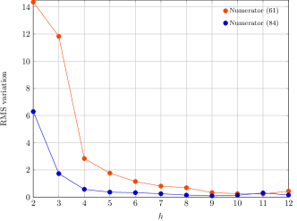
Figure 2: RMS values of $\Delta(\bm{Z},h)$ versus $h$.

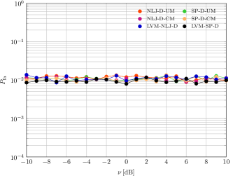
(a) $\bm{m}^{\prime}_{0}=\nu\bm{m}_{0}$

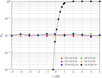
(b) $\bm{\Sigma}^{\prime}_{0}=\gamma\bm{\Sigma}_{0}$

Figure 3: $P_{\text{fa}}$ versus $\nu$ and $\gamma$. In (a) the $P_{\text{fa}}$ is computed assuming $\bm{m}^{\prime}_{0}=\nu\bm{m}_{0}$ and is equal to the nominal value $10^{-2}$ when $\bm{m}^{\prime}_{0}=\bm{m}_{0}$. In (b) the $P_{\text{fa}}$ is computed assuming $\bm{\Sigma}^{\prime}_{0}=\gamma\bm{\Sigma}_{0}$ and is equal to the nominal value $10^{-2}$ when $\bm{\Sigma}^{\prime}_{0}=\bm{\Sigma}_{0}$.

V-B Performance of the NLJ Detection Architectures

The detection performances for the NLJ-D-UM, NLJ-D-CM, and LVM-NLJ-D are shown in Figures 4 and 5, where we plot the $P_{\text{d}}$ curves against the parameter $\gamma$.

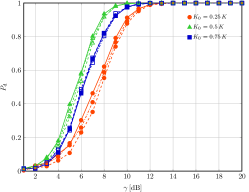
(a) NLJ-D-UM

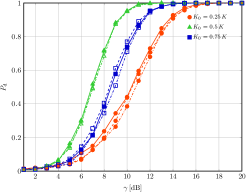
(b) NLJ-D-CM

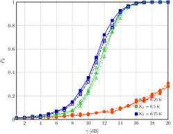
(c) LVM-NLJ-D

Figure 4: $P_{\text{d}}$ versus $\gamma$ for the NLJ-D-UM, NLJ-D-CM, and LVM-NLJ-D assuming $K=24$, $\mbox{SNR}=-30$ dB (solid lines), $\mbox{SNR}=-15$ dB (dashed lines), and $\mbox{SNR}=0$ dB (dot-dashed lines).

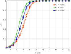
(a) NLJ-D-UM

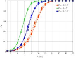
(b) NLJ-D-CM

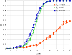
(c) LVM-NLJ-D

Figure 5: $P_{\text{d}}$ versus $\gamma$ for the NLJ-D-UM, NLJ-D-CM, and LVM-NLJ-D assuming $K=32$, $\mbox{SNR}=-30$ dB (solid lines), $\mbox{SNR}=-15$ dB (dashed lines), and $\mbox{SNR}=0$ dB (dot-dashed lines).

Figure 4(a) shows the performance of the NLJ-D-UM assuming $K=24$ and different values for the SNR. As expected, while the SNR does not have a remarkable impact on the performance, the value of $K_{0}$ influences the $P_{\text{d}}$. As a matter of fact, the latter does not increase monotonically with $K_{0}$ and the best performance is obtained for $K_{0}=K/2$. Just to give an example, notice that given $\mbox{\acs{SNR}}=-30\,$dB and $\gamma=8\,$dB, $P_{\text{d}}=0.61$ for $K_{0}=K/4$, $P_{\text{d}}=0.92$ for $K_{0}=K/2$, and $P_{\text{d}}=0.81$ for $K_{0}=3K/4$. The performances of NLJ-D-CM are reported in Figure 4(b) which shares the same parameter values as in the previous figure. The results confirm both the insensitivity of the performance to the SNR and the previously described behavior with respect to the value of $K_{0}$. For instance, in this case, given SNR$=-30\,$dB and $\gamma=8\,$dB, we observe $P_{\text{d}}=0.22$ for $K_{0}=K/4$, $P_{\text{d}}=0.71$ for $K_{0}=K/2$, and $P_{\text{d}}=0.39$ for $K_{0}=3K/4$. From the comparison between Figures 4(a) and 4(b), it turns out that NLJ-D-UM exhibits better performance than the NLJ-D-CM since the former exploits the information related to the actual structure of the error covariance matrix, whereas the latter is designed without assuming any special structure for the covariance matrix. The performance gain of the NLJ-D-UM over the NLJ-D-CM is considerable for $K_{0}=K/4$ and $K_{0}=3K/4$ and becomes less important for $K_{0}=K/2$. Finally, in Figure 4(c), we show the $P_{\text{d}}$ curves associated with the LVM-NLJ-D for $K=24$. The figure points out that this architecture experiences a very poor performance for the case $K_{0}=K/4$ and, generally speaking, its performance is worse than those of the other detectors.

In Figures 5(a)-5(c), we analyze the effect of the sliding window size on the detection performance. In fact, these figures are analogous to the previous three figures except for $K=32$. As expected, in this case, since the number of available data increases, the estimation quality improves leading to better detection performance for all the proposed architectures.

As final remark, it is important to underline that despite the fact that the NLJ-D-CM is designed assuming the most general structure for the covariance matrix, the detection loss with respect to the NLJ-D-UM, whose performance is estimated under perfectly matched design conditions, becomes negligible as $K$ increases. Therefore, we would single out the NLJ-D-CM as an “all-season” architecture capable of operating without any a priori assumption about data correlation.

V-C Performance of the Spoofing Detection Architectures

This last subsection focuses on the performance assessment of the SP-D-UM, SP-D-CM, and LVM-SP-D in terms of probability of spoofing detection. The analysis consider two values of $K$ and three values for the SNR as in the previous subsection. Specifically, Figure 6 assume $K=24$ whereas in Figure 7 $K$ is equal to $32$.

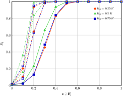
(a) SP-D-UM

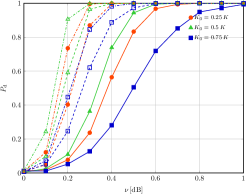
(b) SP-D-CM

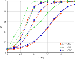
(c) LVM-SP-D

Figure 6: $P_{\text{d}}$ versus $\nu$ for the SP-D-UM, SP-D-CM, and LVM-SP-D assuming $K=24$, SNR$=-30\,$dB (solid lines), SNR$=-15\,$dB (dashed lines), and SNR$=0\,$dB (dot-dashed lines).

(a) SP-D-UM

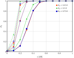
(b) SP-D-CM

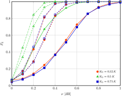
(c) LVM-SP-D

Figure 7: $P_{\text{d}}$ versus $\nu$ for the SP-D-UM, SP-D-CM, and LVM-SP-D assuming $K=32$, SNR$=-30\,$dB (solid lines), SNR$=-15\,$dB (dashed lines), and SNR$=0\,$dB (dot-dashed lines).

Starting from the case $K=24$, we notice that, unlike the performance of the NLJ detectors, the SNR variations significantly affects the $P_{\text{d}}$ that, in this case, increases with the SNR. This behavior can be observed for all the proposed spoofing detectors. For instance, in Figure 6(a), given $\nu=0.2\,$dB and $K_{0}=K/2$, $P_{\text{d}}=0.17$ for SNR$=-30\,$dB, $P_{\text{d}}=0.61$ for SNR$=-15\,$dB, and $P_{\text{d}}=0.94$ for SNR$=0\,$dB. Analogous remarks hold also for Figures 6(b) and 6(c). As for the loss of SP-D-CM with respect to the SP-D-UM due to the more general design assumptions of the former with respect to the latter, in this case, it is less important than that observed in the numerical examples of the previous subsection. Moreover, notice that, differently from the LVM-NLJ-D, the $P_{\text{d}}$ curves associated with the LVM-SP-D achieve a value greater than $0.9$ for each considered value of $K_{0}$. Finally, in Figure 7 we evaluate the effect of $K$ on the detection performance that, again, improves as $K$ increases. Another important aspect to be underlined is that for high $K$ values, the $P_{\text{d}}$ variation induced by $K_{0}$ reduces.

Summarizing, also in the presence of a spoofing attacks, we select the SP-D-CM as the suggested solution against this kind of attacks since it accounts for a more general structure for the measurement covariance matrix and the loss with respect to the SP-D-UM becomes negligible for high values of $K$.

VI Conclusions

In this paper we have addressed the problem of detecting an attack to the location services provided by the next generation communication networks. The proposed strategies have been conceived for high-level location data in agreement with 5G standardization work. At the design stage, this problem has been formulated as a binary hypothesis test accounting for possible correlation among the measurements and solved resorting to GLRT-based design procedures as well as the LVM. The analysis conducted on simulated data has singled out the NLJ-D-CM and the SP-D-CM as an effective means to cope with NLJ and spoofing attacks since they represent a good compromise between detection performance and capability of operating without any assumption on data correlation.

Future research tracks might include the development of an architecture capable of classifying and detecting which kind of attack is in course also accounting for more sophisticated jamming attackers.

Anomaly Detection Algorithms for Location Security in 5G Scenarios Wgroup
Version: V07–
Time:

References

- [1] N. Al-Falahy and O. Y. Alani, “Technologies for 5G Networks: Challenges and Opportunities,” IT Professional, vol. 19, no. 1, pp. 12–20, 2017.
- [2] Study on NR positioning support, 3rd Generation Partnership Project 3GPP™ ETSI TR 138 955 V16.0.0, Dec. 2019, release 16.
- [3] LTE Positioning Protocol (LPP), 3rd Generation Partnership Project 3GPP™ 3GPP TS 37.355 V16.2.0 (2020-09), Sep. 2020, release 16.
- [4] NG Radio Access Network (NG-RAN); Stage 2 functional specification of User Equipment (UE) positioning in NG-RAN, 3rd Generation Partnership Project 3GPP™ 3GPP TS 38.305 V16.2.0 (2020-09), Sep. 2020, release 16.
- [5] B. Li, Z. Fei, and Y. Zhang, “UAV Communications for 5G and Beyond: Recent Advances and Future Trends,” IEEE Internet of Things Journal, vol. 6, no. 2, pp. 2241–2263, 2019.
- [6] F. Raissi, S. Yangui, and F. Camps, “Autonomous Cars, 5G Mobile Networks and Smart Cities: Beyond the Hype,” in 2019 IEEE 28th International Conference on Enabling Technologies: Infrastructure for Collaborative Enterprises (WETICE), 2019, pp. 180–185.
- [7] R. Ma, J. Cao, D. Feng, H. Li, B. Niu, F. Li, and L. Yin, “A Secure Authentication Scheme for Remote Diagnosis and Maintenance in Internet of Vehicles,” in 2020 IEEE Wireless Communications and Networking Conference (WCNC), 2020, pp. 1–7.
- [8] M. Lichtman, R. P. Jover, M. Labib, R. Rao, V. Marojevic, and J. H. Reed, “Lte/lte-a jamming, spoofing, and sniffing: threat assessment and mitigation,” IEEE Communications Magazine, vol. 54, no. 4, pp. 54–61, 2016.
- [9] F. M. Aziz, J. S. Shamma, and G. L. Stüber, “Resilience of lte networks against smart jamming attacks: Wideband model,” in 2015 IEEE 26th Annual International Symposium on Personal, Indoor, and Mobile Radio Communications (PIMRC), 2015, pp. 1344–1348.
- [10] R. Piqueras Jover, “Security attacks against the availability of lte mobility networks: Overview and research directions,” in 2013 16th International Symposium on Wireless Personal Multimedia Communications (WPMC), 2013, pp. 1–9.
- [11] D. Rupprecht, K. Kohls, T. Holz, and C. Pöpper, “Breaking LTE on layer two,” in IEEE Symposium on Security & Privacy (SP). IEEE, May 2019.
- [12] S. F. Mjølsnes and R. F. Olimid, “Easy 4g/lte imsi catchers for non-programmers,” 2017.
- [13] R. M. Rao, S. Ha, V. Marojevic, and J. H. Reed, “Lte phy layer vulnerability analysis and testing using open-source sdr tools,” 2017.
- [14] R. Borgaonkar, L. Hirschi, S. Park, and A. Shaik, “New privacy threat on 3g, 4g, and upcoming 5G aka protocols,” Proceedings on Privacy Enhancing Technologies, vol. 2019, no. 3, pp. 108–127, 2019.
- [15] A. Shaik, R. Borgaonkar, S. Park, and J.-P. Seifert, “New vulnerabilities in 4G and 5G cellular access network protocols: Exposing device capabilities,” in Proceedings of the 12th Conference on Security and Privacy in Wireless and Mobile Networks, ser. WiSec ’19. New York, NY, USA: Association for Computing Machinery, 2019, p. 221–231. [Online]. Available: https://doi.org/10.1145/3317549.3319728
- [16] A. Shaik, R. Borgaonkar, N. Asokan, V. Niemi, and J.-P. Seifert, “Practical attacks against privacy and availability in 4g/lte mobile communication systems,” arXiv preprint arXiv:1510.07563, 2015.
- [17] I. Palamà, F. Gringoli, G. Bianchi, and N. B. Melazzi, “The diverse and variegated reactions of different cellular devices to imsi catching attacks,” in Proceedings of the 14th International Workshop on Wireless Network Testbeds, Experimental Evaluation & amp; Characterization, ser. WiNTECH’20. New York, NY, USA: Association for Computing Machinery, 2020, p. 80–86. [Online]. Available: https://doi.org/10.1145/3411276.3412191
- [18] R. P. Jover, “Lte security, protocol exploits and location tracking experimentation with low-cost software radio,” 2016.
- [19] S. Hussain, O. Chowdhury, S. Mehnaz, and E. Bertino, “Lteinspector: A systematic approach for adversarial testing of 4G lte,” in Proc. of Network and Distributed System Security Symposium (NDSS), 01 2018.
- [20] C. Yu, S. Chen, Z. Cai, and J. Díaz-Verdejo, “Lte phone number catcher: A practical attack against mobile privacy,” Sec. and Commun. Netw., vol. 2019, Jan. 2019. [Online]. Available: https://doi.org/10.1155/2019/7425235
- [21] Study on 5G security enhancements against false base stations, 3rd Generation Partnership Project 3GPP™ ETSI 3GPP TR 33.809 V0.11.0 (2020-10), Oct. 2020, release 17.
- [22] Y. Arjoune and S. Faruque, “Smart Jamming Attacks in 5G New Radio: A Review,” in 2020 10th Annual Computing and Communication Workshop and Conference (CCWC), 2020, pp. 1010–1015.
- [23] 3GPP System Architecture Evolution (SAE)-Security Architecture, 3rd Generation Partnership Project 3GPP™ Sep. 2018, release 15.
- [24] M. Liyanage, I. Ahmad, A. B. Abro, A. Gurtov, and M. Ylianttila, A Comprehensive Guide to 5G Security, 1st ed. New Jersey, USA: Wiley, 2017.
- [25] R. Morales-Ferre, P. Richter, E. Falletti, A. de la Fuente, and E. S. Lohan, “A Survey on Coping With Intentional Interference in Satellite Navigation for Manned and Unmanned Aircraft,” IEEE Communications Surveys Tutorials, vol. 22, no. 1, pp. 249–291, 2020.
- [26] D. Margaria, B. Motella, M. Anghileri, J. Floch, I. Fernandez-Hernandez, and M. Paonni, “Signal Structure-Based Authentication for Civil GNSSs: Recent Solutions and Perspectives,” IEEE Signal Process. Mag., vol. 34, no. 5, pp. 27–37, 2017.
- [27] L. Heng, J. J. Makela, A. D. Domínguez-García, R. B. Bobba, W. H. Sanders, and G. X. Gao, “Reliable GPS-based timing for power systems: A multi-layered multi-receiver architecture,” in 2014 Power and Energy Conf. at Illinois (PECI), Champaign, IL, Feb. 2014, pp. 1–7.
- [28] K. Grover, A. Lim, and Q. Yang, “Jamming and Anti-Jamming Techniques in Wireless Networks: A Survey,” Int. J. Ad Hoc Ubiquitous Comput., vol. 17, no. 4, p. 197 C215, Dec. 2014.
- [29] M. Lichtman, T. Czauski, S. Ha, P. David, and J. H. Reed, “Detection and Mitigation of Uplink Control Channel Jamming in LTE,” in 2014 IEEE Military Communications Conference, Oct 2014, pp. 1187–1194.
- [30] R. D. Pietro and G. Oligeri, “Jamming mitigation in cognitive radio networks,” IEEE Network, vol. 27, no. 3, pp. 10–15, 2013.
- [31] F. M. Aziz, J. S. Shamma, and G. L. St ber, “Jammer-Type Estimation in LTE With a Smart Jammer Repeated Game,” IEEE Transactions on Vehicular Technology, vol. 66, no. 8, pp. 7422–7431, 2017.
- [32] K. Firouzbakht, G. Noubir, and M. Salehi, “On the Performance of Adaptive Packetized Wireless Communication Links Under Jamming,” IEEE Transactions on Wireless Communications, vol. 13, no. 7, pp. 3481–3495, 2014.
- [33] O. A. Topal, S. Gecgel, E. M. Eksioglu, and G. K. Kurt, “Identification of smart jammers: Learning-based approaches using wavelet preprocessing,” Physical Communication, vol. 39, no. 101029, 2020.
- [34] J. Vinogradova, E. Bj 0 2rnson, and E. G. Larsson, “Detection and mitigation of jamming attacks in massive MIMO systems using random matrix theory,” in 2016 IEEE 17th International Workshop on Signal Processing Advances in Wireless Communications (SPAWC), 2016, pp. 1–5.
- [35] H. L. Van Trees, Optimum Array Processing (Detection, Estimation, and Modulation Theory, Part IV). John Wiley & Sons, 2002.
- [36] H. Akhlaghpasand, S. M. Razavizadeh, E. Bj 0 2rnson, and T. T. Do, “Jamming Detection in Massive MIMO Systems,” IEEE Wireless Communications Letters, vol. 7, no. 2, pp. 242–245, 2018.
- [37] A. Conti, S. Mazuelas, S. Bartoletti, W. C. Lindsey, and M. Z. Win, “Soft information for localization-of-things,” Proc. IEEE, vol. 107, no. 11, pp. 2240 – 2264, Nov. 2019.
- [38] S. Mazuelas, A. Conti, J. C. Allen, and M. Z. Win, “Soft range information for network localization,” IEEE Trans. Signal Process., vol. 66, no. 12, pp. 3155–3168, Jun. 2018.
- [39] M. Z. Win, Y. Shen, and W. Dai, “A theoretical foundation of network localization and navigation,” Proc. IEEE, vol. 106, no. 7, pp. 1136–1165, Jul. 2018, special issue on Foundations and Trends in Localization Technologies.
- [40] K. Murphy, Machine Learning: A Probabilistic Perspective, ser. Adaptive Computation and Machine Learning series. MIT Press, 2012.
- [41] L. Childs, A Concrete Introduction to Higher Algebra, ser. Undergraduate Texts in Mathematics. Springer New York, 2008.
- [42] R. J. Muirhead, Aspects of multivariate statistical theory. John Wiley & Sons, 2009.
- [43] T. Cover and J. Thomas, Elements of Information Theory. Wiley, 2012.
- [44] R. A. Horn and C. R. Johnson, Matrix Analysis. Cambridge University Press, 1985.
- [45] J. A. del Peral-Rosado, O. Renaudin, C. Gentner, R. Raulefs, E. Dominguez-Tijero, A. Fernandez-Cabezas, F. Blazquez-Luengo, G. Cueto-Felgueroso, A. Chassaigne, D. Bartlett, F. Grec, L. Ries, R. Prieto-Cerdeira, J. A. Lopez-Salcedo, and G. Seco-Granados, “Physical-layer abstraction for hybrid gnss and 5g positioning evaluations,” in 2019 IEEE 90th Vehicular Technology Conference (VTC2019-Fall), 2019, pp. 1–6.
- [46] E. Rastorgueva-Foi, M. Costa, M. Koivisto, K. Lepp nen, and M. Valkama, “User positioning in mmw 5g networks using beam-rsrp measurements and kalman filtering,” in 2018 21st International Conference on Information Fusion (FUSION), 2018, pp. 1–7.