Non-Fermi liquid behavior in the Sachdev-Ye-Kitaev model for a one dimensional incoherent semimetal

Abstract

We study a two-band dispersive Sachdev-Ye-Kitaev (SYK) model in 1 + 1 dimension. We suggest a model that describes a semimetal with quadratic dispersion at half-filling. We compute the Green’s function at the saddle point using a combination of analytical and numerical methods. Employing a scaling symmetry of the Schwinger-Dyson equations that becomes transparent in the strongly dispersive limit, we show that the exact solution of the problem yields a distinct type of non-Fermi liquid with sublinear $\rho\propto T^{2/5}$ temperature dependence of the resistivity. A scaling analysis indicates that this state corresponds to the fixed point of the dispersive SYK model for a quadratic band touching semimetal.

I INTRODUCTION

Sachdev-Ye-Kitaev (SYK_q) models describe strongly interacting fermions with infinite range, $q-$body, random all-to-all interactions. The $0+1$ dimensional SYK_q dot model Sachdev ; Sachdev2 exhibits an approximate conformal symmetry in the infrared, is exactly solvable in the limit of a large number of fermion flavors, saturates the bound on quantum chaos and are dual to gravitational theories in $1+1$ dimensions. Stanford ; Stanford-1 ; Stanford-2 . Useful connections to the black hole information problem have also been established Stanford-3 .

In these models, approximate conformal symmetry in the strong coupling/low frequency regime leads to power law behavior of correlation functions. In the SYK₄ model, the zero temperature two-point correlation function decays as $G\left(\omega\right)\sim 1/\sqrt{\omega}$, with $\omega$ the frequency. Finite temperature Green’s functions can be then obtained by appealing to conformal symmetry Sachdev . In dispersive versions of the SYK model, they result in the linear temperature dependence of the dc resistivity, $\rho\propto T$, a characteristic feature of strange metal phases. It was originally conjectured that the linear scaling of the scattering rate in the strange metal phase was due to hyperscaling in the proximity of a quantum critical point buried inside the superconducting phase. Recent momentum resolved electron energy spectroscopy experiments in the cuprates revealed the emergence of a mysterious momentum independent energy scale nearly one order of magnitude larger than the temperature range of the quantum critical fan Mitrano ; Husain , at odds with conventional quantum critical theories. One may speculate Zaanen ; Patel3 ; Sachdev-1 ; Volovik ; cha that the origin of the strange metal phase could be related to aspects of the physics of incoherent metals.

Various lattice generalizations Zhang ; Balents ; Sachdev-1 ; Senthil ; Shenoy ; Ben-Zion of the dot model comprising of connected SYK dots have been recently proposed in the regime where the SYK coupling is the dominant energy scale of the problem. The general idea behind many of those extensions is to build on the solution of the dot model including lattice effects perturbatively. Weakly dispersive versions of the SYK model were used to describe incoherent or ‘Planckian’ metals which lack well defined quasiparticles Patel2 ; Volovik ; Dumitrescu . These incoherent metals typically have a crossover between the incoherent high temperature regime and a low temperature Fermi liquid behaviorBalents ; Senthil . The crossover energy scale between the two regimes is set by $t^{2}/J$, with $t$ proportional to the band width and $J\gg t$ the SYK coupling. In the low temperature regime, the coherence of the quasiparticles is restored by the presence of a large Fermi surface. Semimetals, on the other hand, abridge a large class of gapless multiband systems that lack a Fermi surface. One could ask what is the nature of the normal state in a disordered semimetal with random local couplings.

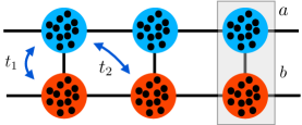
Figure 1: Dispersive SYK ladder model: The unit cell contains two sites, one for each chain (color). Each color site hosts $N$ complex fermions, which interact locally through random couplings. We assume that hopping is only allowed between different color sites, with $t_{1}$ the NN hopping and $t_{2}$ the NNN one. The two-band quadratic dispersion in Eq. (3) can be obtained by tuning $t_{1}=-2t_{2}=t$, with $m=2/(ta^{2})$ the effective mass of the fermions, where $a$ is the lattice constant.

Motivated by these ideas, we study a 1D ladder with local random couplings at every unit cell, as shown in Fig. 1. The hopping amplitudes between lattice sites is finely tuned such that this system describes a half-filled semimetal with quadratic dispersion and local SYK couplings. The weakly dispersive limit $t^{2}/J\ll T\ll J$ has approximate conformal invariance and recovers the usual SYK transport behavior, as expected. In the strongly dispersive regime, $T\ll t^{2}/J$, the scaling symmetry of the problem becomes transparent, albeit the absence of conformal symmetry. In this limit, the incoherent regime extends down to zero frequency and temperature, unlike in the more conventional metallic case. We show that the resistivity of this model has a sublinear scaling with temperature,

$$\rho\propto T^{2/5},$$ (1)

whereas the Lorentz ratio $L=\kappa/(\sigma T)\approx 3.2$ is fairly close to the value expected for a Fermi liquid, $L=\pi^{2}/3$. We find through a scaling argument that when the system starts from the SYK fixed point at high temperature, it flows towards a distinct non-Fermi liquid (NFL) fixed point at zero temperature. At intermediate energy scales, away from the low temperature fixed point, the system crosses over from a “Planckian” semimetal to an incoherent NFL with sublinear temperature scaling of the resistivity.

This paper is organized in the following way: in section II we introduce the lattice model of a 1D ladder of SYK quantum dots that behaves as a 1D semimetal with quadratic dispersion. In section III we address the Green’s function of this system at zero and finite temperature. In the strongly dispersive regime ($T\ll t^{2}/J$), where conformal symmetry is not present, we numerically extract the finite temperature scaling functions of the Green’s function and of the self-energy. In section IV, we discuss a scaling analysis of the problem and the crossover between the high temperature incoherent Planckian regime and the low temperature NFL one. In section V we address the temperature scaling of the dc resistivity of the model. Finally, in section VI we present our conclusions.

II MODEL

We consider $N-$flavors of complex fermions hopping on an 1D lattice. Each lattice site hosts an SYK dot with random, site dependent interactions $J_{ijk\ell}^{x}$ between them. The indexes $i,j,k,\ell=1,..,N$ label the $N-$flavors/colors per site. We start from a 1D ladder shown in Fig. 1, with two sites per unit cell, shown in blue and red. Allowing hopping processes between blue and red sites only, the Hamiltonian of the kinetic term can be written as

$$\hat{\mathcal{H}}_{0}=\int_{k}\sum_{\nu}f(k)\psi_{k,i,\nu}^{\dagger}\left(\sigma_{x}\right)_{\nu,\nu^{\prime}}\psi_{k,i,\nu^{\prime}},$$ (2)

where

$$f(k)=t_{1}+2t_{2}\cos(ka),$$ (3)

with $t_{1}$ and $t_{2}$ the hopping between nearest neighbors (NN) and second nearest neighbors (NNN) respectively among different color sites, and $\int_{k}\equiv a(2\pi)^{-1}\int_{-\Lambda}^{\Lambda}\text{d}k$ with $\Lambda=\pi/a$ the ultraviolet cutoff. $\psi_{i,\nu}$ is a two-component spinor in the site basis of the unit cell $\nu=a,b$ and $\sigma_{x}$ is the real off-diagonal Pauli matrix in that basis. Fine tuning the hopping constants to $t_{1}=-2t_{2}=t$, then

$$\mathcal{H}_{0}=\int_{k}\sum_{i\nu}\frac{k^{2}}{2m}\psi_{k,i,\nu}^{\dagger}\left(\sigma_{x}\right)_{\nu\nu^{\prime}}\psi_{k,i,\nu^{\prime}},$$ (4)

in the continuum limit ($k\ll 1/a$), with $m^{-1}=ta^{2}/2$. The dispersion of this model has two quadratic bands touching at a single point $k=0$, as shown in Fig. 2. At half filling, the band lacks a Fermi momentum and behaves as a 1D semimetal. In the following, we assume the band to be half filled and set $a\to 1$.

Figure 2: Finely tuned energy dispersion for the ladder model illustrated in Fig. 1. The half-filled band describes a 1D semimetal with parabolic band touching at $k=0$.

These fermions interact via a local, instantaneous two body SYK interaction,

$$\mathcal{H}_{\text{SYK}}=\frac{1}{\left(N\right)^{\frac{3}{2}}}\!\!\sum_{\nu\nu^{\prime},ijk\ell}\int_{x}J_{ijk\ell}^{x}\psi_{x,i,\nu}^{\dagger}\psi_{x,j,\nu^{\prime}}^{\dagger}\psi_{x,k,\nu^{\prime}}\psi_{x,\ell,\nu}$$ (5)

with random, color site independent matrix elements $J_{ijk\ell}^{x}$ that are properly antisymmetrized with $J_{ijk\ell}^{x}=-J_{jik\ell}^{x}=-J_{ij\ell k}^{x}.$ As in the other SYK models, we take these to be complex Gaussian distributed coupling with a zero mean value $\langle\langle J_{ijk\ell}^{x}\rangle\rangle=0$ and variance $\langle\langle|J_{ijk\ell}^{x}|^{2}\rangle\rangle=J^{2}/8.$

The standard method to study the current problem is the imaginary time path integral formalism, where the partition function is given by $\mathcal{Z}=\int\left[\mathcal{D}\bar{\psi}\mathcal{D}\psi\right]\mathrm{e}^{-\mathcal{S}}$, where $\mathcal{S}=\mathcal{S}_{0}+\mathcal{S}_{\text{SYK}}$, with

$$\mathcal{S}_{0}=\int_{\tau,x}\sum_{\ell,\nu}\bar{\psi}_{\ell,\nu}\left(\tau,x\right)\left[\partial_{\tau}-\left(\sigma_{x}\right)_{\nu\nu^{\prime}}\frac{\partial_{x}^{2}}{2m}\right]\psi_{\ell,\nu^{\prime}}\left(\tau,x\right).$$ (6)

We define $\int_{\tau}\equiv\int_{0}^{\beta}\text{d}\tau$, with $\beta=1/T$, and $\mathcal{S}_{\text{SYK}}$ the corresponding two body action of (5) with with same time Grassmann fields $\bar{\psi}(\tau,x)$ and $\psi(\tau,x)$. In order to deal with the disorder, we use the replica trick and average over disorder realizations. This procedure amounts to an annealed approximationRosenhaus . Using

$$\langle\langle e^{-\sum_{ijk\ell}J_{ijk\ell}A_{ijk\ell}}\rangle\rangle=e^{J^{2}\sum_{ijk\ell}\bar{A}_{ijk\ell}A_{ijk\ell}}$$ (7)

and defining the Green’s function

$$\hat{G}_{\nu\nu^{\prime}}\left(\tau,x\right)=-\frac{1}{N}\sum_{\ell=1}^{N}\langle T[\psi_{\nu,\ell}\left(0,0\right)\bar{\psi}_{\nu^{\prime},\ell}\left(x,\tau\right)]\rangle,$$ (8)

the integration over the fermionic fields results in the saddle point action,

$$\mathcal{S}_{\text{eff}}=-\log\det\left[\delta\left(\tau-\tau^{\prime}\right)\delta\left(x-x^{\prime}\right)\left(\partial_{\tau}+\sigma_{x}\left(i\partial_{x}\right)^{2}\right)+\hat{\Sigma}\left(x-x^{\prime},\tau-\tau^{\prime}\right)\right]\\ -\frac{J^{2}}{8}\int_{\tau,\tau^{\prime}}\text{tr}\hat{G}^{2}\left(0,\tau-\tau^{\prime}\right)\text{tr}\hat{G}^{2}\left(0,\tau^{\prime}-\tau\right)-\int_{x,x^{\prime}}\int_{\tau,\tau^{\prime}}\text{tr}\left[\hat{\Sigma}\left(x-x^{\prime},\tau-\tau^{\prime}\right)\hat{G}\left(x^{\prime}-x,\tau^{\prime}-\tau\right)\right],$$ (9)

where $\hat{\Sigma}\left(x-x^{\prime},\tau-\tau^{\prime}\right)$ is the self-energy. The action can be minimized exactly in $\hat{G}$ and $\hat{\Sigma}$ in the large-$N$ limit. Following the minimization, the solutions form a set of Schwinger-Dyson equations

$$\hat{G}^{-1}\left(i\omega_{n},k\right)=i\omega_{n}-\frac{k^{2}}{2m}\sigma_{x}-\hat{\Sigma}\left(i\omega_{n},k\right),$$ (10)

and

$$\hat{\Sigma}\left(\tau,x\right)=-\frac{J^{2}}{2}\delta(x)\hat{G}\left(-\tau,0\right)\mathrm{tr}\!\left[\hat{G}\left(\tau,0\right)\hat{G}\left(\tau,0\right)\right],$$ (11)

The self-energy $\hat{\Sigma}\left(i\omega_{n},k\right)\equiv\hat{\Sigma}\left(i\omega_{n}\right)$ is therefore momentum independent, reflecting the $x-$dependence of the couplings $J_{ijk\ell}^{x}$. The disorder averaged SYK term is uncorrelated and purely local. We denote the Fourier transform of the momentum independent self-energy as $\hat{\Sigma}\left(\tau\right)$. We also denote

$$\hat{\mathcal{G}}(\tau)\equiv\hat{G}(\tau,0)=\int_{k}\hat{G}(\tau,k)$$ (12)

for the momentum integrated Green’s function.

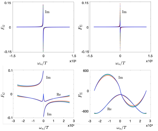
Figure 3: Scaling functions for the Green’s function ($F_{G}$) and the self-energy ($F_{\Sigma}$) versus Matsubara frequency $\omega_{n}$ normalized by temperature $T$. Top row: numerical solution of Eq. (14) and (16) for $F_{G}$ and $F_{\Sigma}$ in the SYK limit for various temperatures, namely $T=10,\,20$ and $30$ (green line, blue and red, respectively). $\beta=T^{-1}$and $J=100$ are set in units of $2m$ with $a\to 1$ ($\Lambda=\pi$). In this case, the Green’s function and self energy are purely imaginary and admit an analytical solution [see Eq. (17)]. Bottom row: numerical solution of Eqs. (14) and (25), in the strongly dispersive regime. The real and imaginary parts of the scaling functions were computed at various temperatures, namely $\beta=1/T=256,\,64$ and $4$ (green line, blue and red, respectively). All curves nearly coincide at low frequencies, where the scaling functions are expected to be temperature independent.

III GREEN’S FUNCTION

If one takes the ansatz for the Green’s function, $\hat{G}(\tau)=\mathcal{G}(\tau)\sigma_{x}$, the self energy then has to be of the form $\hat{\Sigma}(\tau)=\Sigma(\tau)\sigma_{x}$. As in usual SYK models, we make the usual infrared assumption $i\omega_{n}\ll\Sigma(i\omega_{n})$. The Schwinger Dyson equations (10) and (11) can be written as

$$\mathcal{G}(i\omega_{n}) =-\int_{k}\frac{1}{\frac{k^{2}}{2m}+\Sigma(i\omega_{n})}$$

$$=-\frac{\sqrt{2m}}{\pi\sqrt{\Sigma(i\omega)}}\text{tan}^{-1}\left(\frac{\Lambda}{\sqrt{2m}\sqrt{\Sigma(i\omega)}}\right),$$ (13)

and

$$\Sigma(\tau)=-J^{2}\mathcal{G}^{2}(\tau)\mathcal{G}(-\tau),$$ (14)

There are two limits of particular interest. As it will be clear in the next section, one is the intermediate frequency limit $t^{2}/J\ll\omega\ll J$, where the argument of the $\tan^{-1}(y)$ function,

$$y\equiv\frac{\Lambda}{\sqrt{2m}\sqrt{\Sigma(i\omega)}}$$ (15)

is small. This regime corresponds to the weakly dispersive limit, which recovers the physics of the $0+1$ dimensional SYK dot. The other is the strongly dispersive regime, $\omega\ll t^{2}/J$, where $y\gg 1$. We show that this limit is exactly solvable and leads to a different NFL regime.

III.1 Weakly dispersive limit

In this weakly dispersive limit ($y\ll 1)$, the SYK physics dominates and typically one obtains a fully incoherent system with a linear in $T$ dc resistivity. In that regime, Eq. (13) becomes

$$\mathcal{G}(i\omega_{n})\approx-\frac{1}{\pi}\frac{\Lambda}{\Sigma\left(i\omega_{n}\right)}.$$ (16)

The Schwinger-Dyson Eq. (14) and (16) have the same form as in the SYK dot model Sachdev . They have conformal/reparametrization invariance, indicating a power law solution at $T=0$.

At zero temperature, Eq. (14) and (16) can be solved by the ansatz $\mathcal{G}\left(i\omega\right)=c_{1}\text{e}^{-i\frac{\pi}{4}}\left(i\omega\right)^{-\frac{1}{2}}$ for the time ordered Green’s function Sachdev . Using this result in Eq. (14) and taking a Fourier transform one finds

$$\Sigma\left(i\omega\right)=-\frac{J^{2}c_{1}^{3}}{\pi}e^{i\frac{\pi}{4}}\,\sqrt{i\omega},$$ (17)

where the constant $c_{1}=\Lambda^{\frac{1}{4}}/\sqrt{J}.$ The zero temperature dispersive Green’s function is

$$G(i\omega,k)=\frac{1}{\Sigma\left(i\omega\right)}-\frac{k^{2}/2m}{\Sigma\left(i\omega\right)^{2}}+\ldots\,.$$ (18)

This solution introduces a perturbative correction to the SYK Green’s function, in the same spirit as in the metallic case Senthil .

To get the finite temperature solutions, one can then use the conformal map, $\tau\rightarrow f\left(\tau\right)=\tan\frac{\pi\tau}{\beta}$. Applying this to the Fourier transform of $\mathcal{G}\left(i\omega\right)$ gives

$$\mathcal{G}\left(\tau\right)=\mathrm{sgn}(\tau)\,c_{1}\sqrt{\frac{1/\beta}{2\sin\pi\tau/\beta}}.$$ (19)

The finite temperature self-energy $\Sigma\left(i\omega_{n}\right)$ can then be obtained from a Fourier transform of (14),

$$\Sigma\left(i\omega_{n}\right)=iJ^{2}c_{1}^{3}\frac{\left(2\pi\right)^{3/2}\sqrt{2}\Gamma\left(\frac{3}{4}+\frac{\omega_{n}\beta}{2\pi}\right)\Gamma\left(-\frac{1}{2}\right)}{\sqrt{\beta}\pi\Gamma\left(\frac{1}{4}+\frac{\omega_{n}\beta}{2\pi}\right)},$$ (20)

with $\omega_{n}$ a Matsubara frequency. The dispersive Green’s function at finite temperature follows from Eq. (16) and (20),

$$G(i\omega_{n},k)=\frac{1}{\Sigma\left(i\omega_{n}\right)}-\frac{k^{2}/2m}{\Sigma^{2}\left(i\omega_{n}\right)}+\ldots\,.$$ (21)

It is well known that the Greens function and self energies in this regime have some convenient scaling properties. Eqs. (14) and (16) admit solutions of the form:

$$\mathcal{G}(i\omega_{n})=(JT)^{-\frac{1}{2}}\Lambda^{-\frac{3}{4}}F_{G}\left(\frac{\omega_{n}}{T}\right)$$ (22)

$$\Sigma(i\omega_{n})=(JT)^{\frac{1}{2}}\Lambda^{\frac{3}{4}}F_{\Sigma}\left(\frac{\omega_{n}}{T}\right)$$ (23)

where $F_{G,\Sigma}$ are scaling functions which are independent of all parameters. The scaling functions are plotted in the top row panels of Fig. 3. They were obtained by numerically solving Eq. (14) and (16) for various temperatures and then stripping away the power law dependence in $T$ and $J$ from the above equations. The results show good agreement with the scaling arguments.

III.2 Strongly dispersive regime

Next we consider the regime where $y\gg 1$. As we will show below, this inequality corresponds to the regime where

$$\omega\ll\frac{t^{2}}{J},$$ (24)

and leads a different kind of NFL behavior compared to weakly dispersive SYK models.

In the $y\gg 1$ regime, the Schwinger-Dyson equation (13) reads

$$\mathcal{G}(i\omega)=-\frac{1}{2}\frac{\sqrt{2m}}{\sqrt{\Sigma(i\omega)}}.$$ (25)

Eq. (14) and (25) admit a power law solution at $T=0,$ given by the ansatz

$$\mathcal{G}(\tau)=C\frac{1}{\left|\tau\right|^{2\Delta}},$$ (26)

where $2\Delta=3/5$, as found in a related model Shenoy , with

$$C=\left[\frac{\Gamma(\frac{1}{5})^{-1}\Gamma(\frac{2}{5})^{-2}}{20\sin^{2}\left(\frac{3\pi}{10}\right)\sin\left(\frac{9\pi}{10}\right)}\right]^{\frac{1}{5}}\approx 0.40.$$ (27)

That solution corresponds to a self-energy

$$\Sigma(i\omega)=C^{\prime}J^{\frac{4}{5}}m^{\frac{3}{5}}\left|\omega\right|^{6\Delta-1}\gg|\omega|,$$ (28)

from equation (14). Explicit verification of this solution follows by Fourier transforming (25),

$$\mathcal{G}(i\omega)=2C\sin\pi\Delta\ \Gamma(1-2\Delta)J^{-\frac{2}{5}}m^{\frac{1}{5}}\left|\omega\right|^{2\Delta-1},$$ (29)

and calculating $\Sigma\left(i\omega\right)$ from (14). The zero-temperature Green’s function is hence

$$\hat{G}(i\omega,k)=\frac{-\sigma_{x}}{\frac{k^{2}}{2m}+C^{{}^{\prime}}J^{\frac{4}{5}}m^{\frac{3}{5}}\left|\omega\right|^{4/5}},$$ (30)

where

$$C^{\prime}=-2C^{3}\sin\left(\frac{9\pi}{10}\right)\Gamma\left(-\frac{4}{5}\right)\approx 0.22.$$ (31)

The Green’s function above describes a distinct type of incoherent semimetal, and is valid all the way down to zero frequency. It contrasts with the result in the coherent $J\to 0$ limit of the ladder problem model ($J/|\omega|\ll 1$), where the Green’s function has a pole with well defined quasiparticles. One needs to analytically continue the above solution and impose physical restrictions to obtain the exact Green’s function.

Note that the linear in $T$ resistivity in SYK models stems from $\Delta=\frac{1}{4}.$ In strongly dispersive semimetals, with $y\gg 1$, finite temperature solutions cannot be obtained using a conformal map on the $T=0$ solution because (14) and (25) do not have the requisite conformal/reparametrization symmetry. Finite temperature solutions to these equations then have to be obtained numerically. However, we still have a scaling symmetry which dictates a certain scaling form for the solutions.

Rewriting (25) in $\tau-$space,

$$\int_{\tau_{1},\tau_{2}}\mathcal{G}(\tau)\mathcal{G}(\tau-\tau_{2})\Sigma(\tau-\tau_{1})=\frac{m}{2}\delta(\tau).$$ (32)

It is easy to see that these equations are invariant under

$$\tau\rightarrow b\tau,\quad\mathcal{G}\rightarrow b^{-\frac{3}{5}}\mathcal{G},\quad\Sigma\rightarrow b^{-\frac{9}{5}}\Sigma.$$ (33)

Under this scaling, $T\rightarrow T/b$ leaving $T\tau$ invariant. With this information, one can see that (14) and (25) admit a solution of the form

$$\mathcal{G}(\tau)=m^{\frac{1}{5}}J^{-\frac{2}{5}}T^{\frac{3}{5}}\tilde{\mathcal{G}}(T\tau)$$ (34)

and

$$\Sigma(\tau)=m^{\frac{3}{5}}J^{\frac{4}{5}}T^{\frac{9}{5}}\tilde{\Sigma}(T\tau).$$ (35)

Equivalently in Fourier space, we find

$$\mathcal{G}(i\omega_{n})=m^{\frac{1}{5}}(JT)^{-\frac{2}{5}}F_{G}\left(\frac{\omega_{n}}{T}\right)$$ (36)

$$\Sigma(i\omega_{n})=m^{\frac{3}{5}}(JT)^{\frac{4}{5}}F_{\Sigma}\left(\frac{\omega_{n}}{T}\right)$$ (37)

where $F_{G,\Sigma}$ are scaling functions that are independent of temperature $T$ and the coupling $J$, with $\omega_{n}$ a Matsubara frequency. The dispersive finite temperature Green’s function of the problem in this regime is

$$\hat{G}^{-1}(i\omega_{n},k)=-\left(\frac{k^{2}}{2m}+m^{\frac{3}{5}}(JT)^{\frac{4}{5}}F_{\Sigma}(\omega_{n}/T)\right)\sigma_{x}.$$ (38)

As shown in the next section, this will suffice to determine the temperature dependence of various transport coefficients. Strictly speaking, the scaling symmetry is only present in the infrared limit of the theory. This means that the exact numerical solutions may violate these scaling forms at very high frequencies. The real and imaginary parts of the numerically obtained scaling functions $F_{G}$ and $F_{\Sigma}$ are plotted in the bottom row of Fig. 3. The plots show good agreement with Eq. (37) even outside the infrared limit.

IV Scaling analysis

After averaging over the disorder, which is spatially uncorrelated, the SYK term in the action has eight fermionic fields, which we symbolically write as

$$\mathcal{S}_{\text{SYK}}=J^{2}\int_{\tau_{1},\tau_{2},x}[\bar{\psi}(\tau_{1},x)\psi(\tau_{1},x)]^{2}[\bar{\psi}(\tau_{2},x)\psi(\tau_{2},x)]^{2}.$$ (39)

Rescaling time as $\tau^{\prime}=\tau/s$ and imposing the SYK coupling $J$ to be marginal, then the fields rescale as $\psi^{\prime}=\psi/s^{\frac{1}{4}}$. As pointed out before Balents ; Senthil , analyzing the problem in the vicinity of the fixed point of the $0+1$ dimensional SYK model $(t=0$), the kinetic term is a relevant perturbation and the hopping parameter grows as $t^{\prime}=t\sqrt{s}$. If one starts from temperature $T$ in the weakly dispersive regime $t\ll J$, the hopping will grow until $t^{\prime}(s_{*})\sim J$ for a rescaling parameter no larger than $s_{*}=J/T$. Hence, the scaling stops at $T=t^{2}/J$. The validity of the incoherent “Planckian” regime requires that

$$T\gg T_{*}=t^{2}/J,$$ (40)

as in the case of incoherent metals with a finite Fermi surface Senthil .

If one continues to lower the temperature further below $T_{*}$, we claim that the system crosses over to a different type of incoherent NFL regime with sublinear temperature scaling of the resistivity, as illustrated in Fig. 4. From the perspective of the Schwinger-Dyson equations (13) and (14), the parameter that controls the crossover between the weakly and the strongly dispersive regimes is

$$y(T)\sim\sqrt{\frac{t}{\Sigma(T)}}.$$ (41)

In the strongly dispersive regime $y(T)\gg 1$, setting $m\sim t^{-1}$, one can write the solution of the finite temperature self-energy (37) as

$$\Sigma(T)\propto t^{-\frac{3}{5}}(JT)^{\frac{4}{5}}\ll t.$$ (42)

This inequality leads to $T\ll T_{*}=t^{2}/J$. In the same way, in the weakly dispersive regime ($y(T)\ll 1$),

$$\Sigma(T)\propto\sqrt{JT}\gg t,$$ (43)

as seen from Eq. (20), implying that $T\gg T_{*}$.

We note that in the case of metals, the $T<T^{*}$ regime was found to realize a Fermi liquid. In the case of a 1D half-filled semimetal with parabolic touching, we showed that the low temperature regime does not lead to a semimetal, but to another type of incoherent NFL, whose transport properties will be addressed in the next section.

Figure 4: Different temperature regimes in the scaling. At temperature $T>T_{*}=t^{2}/J$, the system is close to the $0+1$ dimensional SYK fixed point and shows Planckian behavior, with linear dependence of the resistivity in temperature. Below $T_{*}=t^{2}/J$ the system crosses over towards a distinct type of incoherent NFL, with $\rho\sim T^{\frac{2}{5}}$.

V TRANSPORT

In this section, we look at the electric and thermal conductivities using the above finite temperature solutions. These can be computed using the Kubo formula. The charge current operator for this model is

$$\hat{j}_{e}=\frac{e}{2m}\int_{k}\sum_{i}k\psi_{ki}^{\dagger}\sigma_{x}\psi_{ki}.$$ (44)

The zero frequency conductivity is given by

$$\sigma_{\text{dc}}=\mathrm{lim}_{\omega\to 0}\frac{\mathrm{Im}\mathrm{\mathcal{K}}^{\text{ret}}(\omega)}{\omega},$$ (45)

where $\mathrm{\mathcal{K}}^{\text{ret}}(\omega)$ is the retarded current-current correlation function, $\mathrm{\mathcal{K}}(\tau)=\langle T[\hat{j}_{e}(0,x)\hat{j}_{e}(\tau,x)\rangle$, given by the series of diagrams in Fig. 5. Each diagram displayed in that figure is of order $N$. For instance, in diagram (b) each SYK vertex contributes a factor of $N^{-\frac{3}{2}}$ , while the three independent flavor sums contribute $N^{4}$, making it a total of order $N.$ Diagrams in (b) and (c) vanish because the current vertex is an odd function of momenta. This can be readly seen by noticing that because of the disorder averaging, the summation over momenta through each current vertex can be performed independently, resulting in a zero contribution of those diagrams Georges . The remaining diagram is shown in Fig. 5a. It can be written in terms of the Green’s functions derived before as

$$\mathcal{K}(i\omega_{n})=\frac{Ne^{2}}{(2m)^{2}}T\ \mathrm{tr}\sum_{\nu_{n}}\int_{k}k^{2}\hat{G}(i\nu_{n},k)\hat{G}(i\nu_{n}+i\omega_{n},k).$$ (46)

The transport properties of the weakly dispersive regime recovers the expected behavior of incoherent metals found in Ref. Sachdev-1 ; Senthil , $\sigma_{\text{dc}}\propto 1/T$, and we will focus instead in the strongly dispersive case.

It is usually challenging to sum over Matsubara frequencies in the absence of poles in the Green’s functions. One can circumvent that difficulty by using the spectral representation of the Green’s function

$$\hat{G}(i\omega_{n},k)=\int_{\omega^{\prime}}\frac{\mathcal{\hat{A}}(k,\omega^{\prime})}{i\omega_{n}-\omega^{\prime}},$$ (47)

with

$$\mathcal{\hat{A}}(k,\omega)=\frac{1}{\pi}\sigma_{x}\mathrm{Im}\frac{1}{\frac{k^{2}}{2m}+\Sigma(\omega+i0_{+})}$$ (48)

the spectral function. One arrives at

$$\sigma_{dc}=\frac{Ne^{2}\sqrt{2m}}{\pi^{2}T}\int_{\omega}\frac{\left[\text{Im}\Sigma(\frac{\omega}{T})\right]^{2}}{\cosh^{2}(\frac{\omega}{2T})}\int_{k}\frac{k^{2}}{\left|\frac{k^{2}}{2m}+\Sigma\left(\frac{\omega}{2T}\right)\right|^{4}}.$$ (49)

Equivalently, casting Eq. (49) in terms of the scaling functions (37), the dc conductivity is

$$\sigma_{\text{dc}}(T)=\frac{Ne^{2}}{\sqrt{2m}(JT)^{\frac{2}{5}}}I_{1},$$ (50)

where

$$I_{1}=\frac{1}{\pi^{2}}\int_{0}^{\infty}\text{d}z\frac{\left[\text{Im}F_{\Sigma}(z)\right]^{2}}{\cosh^{2}(\frac{z}{2})}\int_{0}^{\infty}\text{d}y\frac{y^{2}}{\left|y^{2}+F_{\Sigma}\left(z\right)\right|^{4}}$$ (51)

is a dimensionless integral, and $F_{\Sigma}(z)$ the analytically continued scaling function of the self energy.

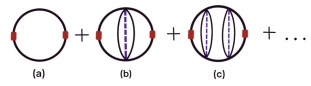
Figure 5: Diagrams that contribute to the current-current correlation function to leading order in $N$ (see text). Red rectangles represent the current vertex. Black lines represent the fermion Green’s function and dotted blue line represents disorder average. Since the current vertex is an odd function of momenta, diagrams (b) and (c) and so on vanish, leaving (a) as the sole contribution in the large-$N$ limit.

A signature property of Fermi liquids is captured by the Lorentz ratio, $L=\kappa/(\sigma T)$, which is the ratio of thermal $(\kappa)$ and electric $(\sigma)$ conductivities. In the particle-hole symmetric model, the thermoelectric contribution to the thermal conductivity, which is proportional to $T/\sigma$, vanishes by symmetry and can be ignored in the computation of $\kappa$ Sachdev-1 ; Patel2 . The energy current, whose correlation function determines the remaining piece of the thermal conductivity, is given by

$$\hat{j}_{E}=\int_{k}\sum_{i}\frac{k}{2m}\psi_{k,i}^{\dagger}\sigma_{x}\partial_{\tau}\psi_{k,i}.$$ (52)

In the present particle-hole symmetric case, the thermal conductivity is then given by the same diagrams as in the case of $\sigma$. Following the same prescription as above,

$$\kappa=\mathrm{lim}_{\omega\rightarrow 0}\frac{\mathrm{\mathcal{K}}_{E}^{\text{ret}}(\omega)}{\omega T},$$ (53)

where $\mathrm{\mathcal{K}}_{E}(\tau)=\langle T[\hat{j}_{E}(0,x)\hat{j}_{E}(\tau,x)\rangle$ is a thermal current-current correlation function. This leads to

$$\kappa=\frac{Ne^{2}}{\sqrt{2m}J^{\frac{2}{5}}}T^{\frac{3}{5}}I_{2},$$ (54)

where

$$I_{2}=\frac{1}{\pi^{2}}\int_{0}^{\infty}\text{d}z\,z^{2}\frac{\text{Im}\left[F_{\Sigma}(z)\right]^{2}}{\cosh^{2}(\frac{z}{2})}\int_{0}^{\infty}\text{d}y\frac{y^{2}}{\left|y^{2}+F_{\Sigma}\left(z\right)\right|^{4}}.$$ (55)

In order to calculate integrals $I_{1}$ and $I_{2}$, one needs to perform a numerical analytical continuation of the scaling functions obtained in section III. In the spirit of SYK models, we compute these integrals assuming the scaling form to be valid over the entire range of frequencies. Numerical analytical continuation is a challenging problem. The numerical integrals were done with the Pade approximation method in the TRIQS library Serene ; TRIQS .

We numerically find that slight variations in the Matsubara scaling forms can significantly affect the integrals $I_{1}$ and $I_{2}$, but their ratio is insensitive to numerical issues with the analytical continuation process in the regime of interest. The Lorentz ratio is

$$L=\frac{\kappa}{T\sigma}=\frac{I_{2}}{I_{1}}\approx 3.2,$$ (56)

which is rather close to the Fermi liquid value of $L_{FL}=\pi^{2}/3.$

VI Discussion

In this work, we studied a simple semimetallic version of a dispersive SYK model in one dimension. Contrary to most studies of dispersive models in the literature Zhang ; Balents ; Sachdev-1 ; Senthil ; Shenoy , we focus on the strongly dispersive limit, which corresponds to the stable fixed point of this problem from the scaling point of view. In this limit, we find that the Schwinger-Dyson equations do not admit an exact analytic finite temperature solution even in the infrared approximation, where it is assumed that $\Sigma(i\omega)\gg i\omega$. In particular, the model does not exhibit conformal symmetry, which makes it difficult to solve the Schwinger-Dyson equations analytically. We solve those equations exactly exploiting the scaling symmetry of the model, combined with numerical calculations. We find that the Greens function and self-energy scale with temperature with a power law of $T^{-\frac{2}{5}}$ and $T^{\frac{4}{5}}$ respectively.

Using this solution to study transport properties, we show that dc resistivity scales with a sublinear power law dependence on temperature, $\rho\sim T^{\frac{2}{5}}.$ We compute the Lorentz ratio $L=\kappa/(\sigma T)$ with the analytically continued scaling functions and find that $L\approx 3.2,$ rather close to that of Fermi liquids. The scaling analysis of this problem indicates that if one starts in the high temperature SYK fixed point of the problem, where $t^{2}/J\ll T\ll J$, the hopping parameter will grow as one scales the temperature down, while the SYK coupling is marginal. The scaling flows towards the strongly dispersive regime, where the Schwinger-Dyson equations indicate the presence of a distinct incoherent NFL regime at $T\ll t^{2}/J$. That contrasts with the behavior of incoherent metals, which have a finite Fermi surface. In the latter, the system flows towards a Fermi liquid at low temperature Senthil .

Those results should be compared with the several lattice models of SYK dots that have been studied recently Sachdev-1 ; Senthil ; Shenoy . Ref. Sachdev-1 ; Senthil studied a lattice of coupled dots in the limit where the SYK coupling $J$ is the highest energy scale. In those cases, the physics of a single dot dominates, with the effects of hopping being perturbative. The $\Sigma\propto\sqrt{\omega}$ scaling of the self energy in this limit ultimately leads to a linear in $T$ dc resistivity.

Among the dispersive SYK models, the one studied in Ref. Shenoy is the closest to ours. They examined a two-band model for arbitrary dimension and dispersion, with a color site dependent SYK interaction, which forces the saddle point solution of the Green’s function to be diagonal but still color site dependent. Their solution for the self-energy is purely imaginary and color site independent, differently from our results. That leads to an approximate conformal symmetry in the problem in the NFL regime, in contrast with our work, where we find that conformal symmetry is absent. In this paper, we focused in the crossover between the regime dominated by the $0+1$ dimensional SYK fixed point and the low temperature NFL regime for a 1D semimetal with parabolic band touching, and addressed the transport properties of this novel state.

Acknowledgements.$-$ We thank A. Haldar for several helpful discussions. BU and GJ acknowledge Carl T. Bush fellowship and NSF grant DMR-2024864 for partial support.

References

- (1) S. Sachdev, Bekenstein-Hawking Entropy and Strange Metals, Phys. Rev. X 5, 041025 (2015).
- (2) S. Sachdev and J. Ye, Gapless Spin-fluid ground state in a random quantum Heisenberg magnet, Phys. Rev. Lett. 70, 3339 (1993).
- (3) S. H. Shenker and D. Stanford, Black holes and the butterfly effect, JHEP 03 (2014).
- (4) S. H. Shenker and D. Stanford, Stringy effects in scrambling, JHEP 05 (2015) 132.
- (5) J. Maldacena, S. H. Shenker, and D. Stanford, A bound on chaos, JHEP 08 (2016)106.
- (6) J. Maldacena, D. Stanford, and Z. Yang, Diving into Traversable Wormholes, Fortschr. Phys. 65, 1700034 (2017).
- (7) M. Mitrano, A. A. Husain, S. Viga, A. Kogar, M. S. Rak, S. I. Rubeck, J. Schmalian, B. Uchoa, J. Schneeloche, R. Zhonge, G. D. Gue, and P. Abbamonte, Anomalous density fluctuations in a strange metal, Proc. Nat. Acad. Sci. 115, 5392 (2018).
- (8) A. A. Husain, M. Mitrano, M. S. Rak, S. Rubeck, B. Uchoa, K. March, C. Dwyer, J. Schneeloch, R. Zhong, G. D. Gu, and P. Abbamonte, Crossover of Charge Fluctuations across the Strange Metal Phase Diagram, Phys. Rev X 9, 041062 (2019).
- (9) J. Zaanen, Planckian dissipation, Minimal viscosity and the transport in cuprate strange metals, SciPost Phys. 6, 061 (2019).
- (10) A. A. Patel and S. Sachdev, Critical strange metal from fluctuating gauge fields in a solvable random model, Phys. Rev. B 98, 125134 (2018).
- (11) P. Cha, N. Wentzell, O. Parcollet, A. Georges, and E.-A. Kim, Linear resistivity and Sachdev-Ye-Kitaev (SYK) spin liquid behavior in a quantum critical metal with spin-1/2 fermions, Proc. Natl. Acad. Sci. USA 117, 18341 (2020).
- (12) G.E. Volovik, Flat band and Planckian metal, JETP Lett. 110, 352-353 (2019).
- (13) A. A. Patel, J. McGreevy, D. P. Arovas, and S. Sachdev, Magnetotransport in a model of a disordered strange metal, Phys. Rev. X 8, 021049 (2018).
- (14) P. Zhang, Dispersive Sachdev-Ye-Kitaev model: band structure and quantum chaos, Phys. Rev. B 96, 205138 (2017).
- (15) X.-Y. Song, C.-M. Jian, and L. Balents, Strongly Correlated Metal Built from Sachdev-Ye-Kitaev Models, Phys. Rev. Lett. 119, 216601 (2017).
- (16) Vladimir Rosenhaus, J. Phys. A: Math. Theor. 52 (2019) 323001
- (17) D. Chowdhury, Y. Werman, E. Berg, and T. Senthil, Translationally Invariant Non-Fermi Liquid Metals with Critical Fermi-Surfaces: Solvable Models, Phys. Rev. X 8, 031024 (2018).
- (18) A. Haldar, S. Banerjee, V. B. Shenoy, Higher-dimensional Sachdev-Ye-Kitaev non-Fermi liquids at Lifshitz transitions, Phys. Rev. B 97, 241106 (2018).
- (19) D. Ben-Zion and J. McGreevy, Strange metal from local quantum chaos, Phys. Rev. B 97, 155117 (2018).
- (20) A.A. Patel and S. Sachdev, Theory of a Planckian metal, Phys. Rev. Lett. 123, 066601 (2019).
- (21) P. T. Dumitrescu, N. Wentzell, A. Georges, and O. Parcollet, Planckian metal at a doping-induced quantum critical point, arXiv:2103.08607 (2021).
- (22) A. Georges, G. Kotliar, W. Krauth, and M. J. Rozenberg, Dynamical mean-field theory of strongly correlated fermion systems and the limit of infinite dimensions, Rev. Mod. Phys. 68, 13 (1996).
- (23) H. J. Vidberg, J. W. Serene, Solving the Eliashberg equations by means of -point Pade approximants, J. Low Temp. Phys. 29, 179–192 (1977).
- (24) O. Parcollet, M. Ferrero, T. Ayral, H. Hafermann, I. Krivenko, L. Messio, and P. Seth, TRIQS: A Toolbox for Research on Interacting Quantum Systems, Comp. Phys. Comm. 196, 398-415 (2015).