Searching for the radiative decay of the cosmic neutrino background with line-intensity mapping

Abstract

We study the possibility to use line-intensity mapping (LIM) to seek photons from the radiative decay of neutrinos in the cosmic neutrino background. The Standard Model prediction for the rate for these decays is extremely small, but it can be enhanced if new physics increases the neutrino electromagnetic moments. The decay photons will appear as an interloper of astrophysical spectral lines. We propose that the neutrino-decay line can be identified with anisotropies in LIM clustering and also with the voxel intensity distribution. Ongoing and future LIM experiments will have—depending on the neutrino hierarchy, transition and experiment considered—a sensitivity to an effective electromagnetic transition moment $\sim 10^{-12}\,-\,10^{-8}\,(m_{i}c^{2}/{0.1\rm eV})^{3/2}\mu_{\rm B}$, where $m_{i}$ is the mass of the decaying neutrino and $\mu_{\rm B}$ is the Bohr magneton. This will be significantly more sensitive than cosmic microwave background spectral distortions, and it will be competitive with stellar cooling studies. As a byproduct, we also report an analytic form of the one-point probability distribution function for neutrino-density fluctuations, obtained from the Quijote simulations using symbolic regression.

Considerable efforts are underway to study the properties of neutrinos, including their masses, mixing angles, and nature (e.g., Dirac or Majorana) [1, 2, 3, 4, 5, 6, 7, 8, 9, 10, 11, 12, 13, 14, 15, 16, 17, 18, 19, 20, 21]. The stability of neutrinos is also of interest. An active massive neutrino $\nu_{i}$ can decay into a lighter eigenstate $\nu_{j}$ and photon, $\gamma$, $\nu_{i}\rightarrow\nu_{j}+\gamma$ with a rate determined by electromagnetic transition moments induced via loops involving gauge bosons. The Standard Model (SM) prediction for the lifetime is $\tau_{\rm SM}=7.1\times 10^{43}m^{-5}_{\rm eV}$ s [22, 23, 24, 25], where $m_{\rm eV}\equiv m_{\nu}c^{2}/{\rm eV}$ is the neutrino mass in eV$/c^{2}$ units, significantly longer than the age of the Universe.

However, new physics beyond the SM (BSM) can enhance neutrino magnetic moments [26, 27, 28, 29, 30, 31, 32, 33, 34] and such modifications have been considered in connection with experimental anomalies, such a possible correlation of solar neutrinos with Solar activity [35, 14], or more recently [33, 34] the $\sim 3\sigma$ excess reported XENON1T [36]. Although many avenues have been proposed (see e.g., Ref. [37] for a review), the most efficient direct laboratory probe of neutrino electromagnetic couplings involves neutrino-electron scattering [38, 7, 8]. Tighter bounds on neutrino electromagnetic moments come from astrophysics. In particular, the strongest constraint comes from the tip of the red giant branch in globular clusters, which is sensitive to the additional energy loss through plasmon decay into two neutrinos [39, 40, 41]. Radiative neutrino decays have also been constrained from measurements of the cosmic microwave background (CMB) spectral distortions [42, 43].

Here we study the use of line-intensity mapping (LIM) to seek photons from radiative decays of neutrinos in the cosmic neutrino background. LIM [44, 45] exploits the integrated intensity at a given frequency induced by a well-identified spectral line to map the three-dimensional distribution of matter in the Universe. Photons from particle decays will appear in these maps as an unidentified line [46] that can be distinguished from astrophysical lines through its clustering anisotropies and through the voxel probability distribution function [47]. We find that LIM has the potential to be significantly more sensitive to radiative decays than current cosmological probes and compete with the strongest bounds to electromagnetic moments coming from astrophysical observations.

While neutrino radiative decays are characterized by the electromagnetic transition moments, LIM experiments are sensitive to the luminosity density $\rho_{\rm L}$ of the photons produced in each point $\boldsymbol{x}$, which, for the decay between the $i$ and $j$ states, is given by

$$\rho_{\rm L}^{ij}(\boldsymbol{x})=(1/6)\rho_{\nu}(\boldsymbol{x})c^{2}\Gamma_{ij}\left(1-m_{j}^{2}/m_{i}^{2}\right)\,,$$ (1)

where $\rho_{\nu}$ is the total neutrino density, $\Gamma_{ij}\equiv\tau_{ij}^{-1}$ is the decay rate, and $m_{i}$ are the neutrino masses. We assume that the density of each state is $1/3$ of the total density, as expected apart from small mass differences and flavor corrections that have negligible consequences for the precision goals of this Letter [48]. The corresponding brightness temperature $T$ at redshift $z$ is

$$\begin{split}T^{ij}(z,\boldsymbol{x})&=\frac{c^{3}(1+z)^{2}\rho_{\rm L}^{ij}(z,\boldsymbol{x})}{8\pi k_{\rm B}f^{3}H(z)}=X_{\rm LT}\rho^{ij}_{\rm L}(z,\boldsymbol{x})=\\ &=(X_{\rm LT}/6)\rho_{\nu}c^{2}\Gamma_{ij}\left(1-m_{j}^{2}/m_{i}^{2}\right)\,,\end{split}$$ (2)

where $H$ is the Hubble expansion and $k_{\rm B}$ is the Boltzmann constant and $f$ is the rest-frame frequency [49]. Thus, the brightness temperature from neutrino decays traces the neutrino density field.

Decay photons are then an emission line with rest-frame frequency given by $f_{ij}=\left(m_{i}^{2}-m_{j}^{2}\right)c^{2}/\left(2h_{\rm P}m_{i}\right)$, where $h_{\rm P}$ is the Planck constant. For $m_{i}/c^{2}\gg T_{\nu}/k_{\rm B}\sim 10^{-4}(1+z)\,{\rm eV}$ (where $T_{\nu}$ is the cosmic neutrino temperature), which holds true for our cases of interest, the neutrinos are non-relativistic and we can neglect the linewidths due to their velocity dispersion. The rest-frame frequency of the emission lines is then uniquely characterized by the neutrino hierarchy and the sum $\sum m_{\nu}$ of neutrino masses, as shown in Fig. 1, with the observed frequency redshifted accordingly. The transitions not included in the figure have a very similar frequency than one of the other two (e.g., $f_{31}\approx f_{32}$ for the normal hierarchy) and are not distinguished hereinafter.

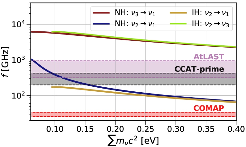
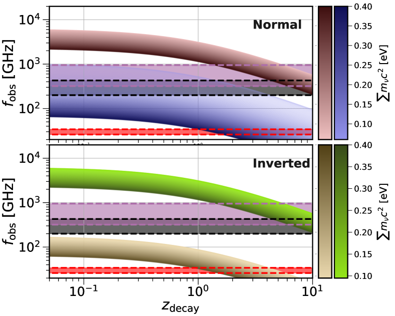
Figure 1: Relation between the sum of neutrino masses and the rest-frame frequency of the photon produced in the decay for normal (NH) and inverted (IH) hierarchies (top) and the corresponding observed frequency. We also show the frequency bands of the experiments considered in both panels with horizontal shaded bands.

We now consider two LIM observables: the power spectrum and the voxel intensity distribution (VID). The observed anisotropic LIM power spectrum associated to the neutrino decay between $i$ and $j$ states is [50, 47]

$$P_{ij}(k,\mu)=W(k,\mu)X_{\rm LT}^{2}\langle\rho_{\rm L}^{ij}\rangle^{2}F^{2}_{\rm rsd}(k,\mu)P_{\rm\nu}(k)\,,$$ (3)

where $k$ is the modulus of the Fourier mode, $\mu\equiv\boldsymbol{k}\cdot\boldsymbol{k}_{\parallel}/k^{2}$ is the cosine of the angle between the Fourier mode and the line of sight, $W$ is a window function modeling the effects from instrumental resolution and finite volume observed, the brackets $\langle\rangle$ denote the spatial mean, $F_{\rm RSD}$ is a redshift-space distortions factor [50], $P_{\rm\nu}$ is the neutrino power spectrum, computed using CAMB [51], and all redshift dependence is implicit. We consider the Legendre multipoles of the LIM power spectrum with respect to $\mu$ up to the hexadecapole.

Experiment	COMAP 1 (2)	CCAT-prime	AtLAST
Line	CO	CII	CII
Freq. band [GHz]	24-36	200-240, 260-300, 330-370, 388-428	315-376, 376-470, 470-620, 620-920
Spectral resolution	4000	100	1000
Ang. resolution [”]	240	57, 45, 35, 30	4.4, 3.6, 2.8, 2.0
Sky coverage [deg2]	2.25 (60)	8	7500
Voxel noise	39 (69) $\mu$K	(0.6, 1.0, 2.5, 5.7)$\times 10^{4}$ Jy/sr	(0.4, 0.7, 1.4, 3.9)$\times 10^{5}$ Jy/sr

Table 1: Instrumental specifications used. Each independent frequency band is separated by commas. CII observations use the convention for specific intensity instead of brightness temperature. We combine 30$\times$30 pixels for VID analyses with AtLAST. More details can be found in Ref. [47].

Similarly, the VID is related to the probability distribution function (PDF) $\mathcal{P}_{\breve{\rho}}$ of the normalized total neutrino density $\breve{\rho}_{\rm\nu}\equiv\rho_{\rm\nu}/\langle{\rho}_{\rm\nu}\rangle$, as $\mathcal{P}_{ij}(T)=\mathcal{P}_{\breve{\rho}}(\breve{\rho}_{\rm\nu})/\langle T^{ij}\rangle$. We estimate the neutrino density PDF from high-resolution simulations of the Quijote simulation suite [52], that model the gravitational evolution of more than 2 billion cold dark matter and neutrino particles in a comoving box of $(1~{}h^{-1}{\rm Gpc})^{3}$ volume. Degenerate neutrino mass eigenstates are assumed.

First, neutrino particle positions are assigned to a regular grid with $1500^{3}$ voxels employing the cloud-in-cell mass-assignment scheme. Next, the 3D field is convolved with a Gaussian kernel of a given width. Then, the PDF is estimated by computing the fraction of voxels with a given $\breve{\rho}_{\nu}$. We do this for $\sum m_{\nu}c^{2}=\{0.1,\,0.2,\,0.\,4\}\,{\rm eV}$, at $z=\{0,\,0.5,\,1,\,2,\,3,\,4,\,5,\,6,\,7,\,8,\,9\}$ and for 6 smoothing scales $\{2,\,3,\,4,\,5,\,7.5,\,10\}\,h^{-1}{\rm Mpc}$. We have checked that the computed PDFs, in the range of interest for this study, are converged in our simulations. Note that all dependences can be condensed in the root-mean square $\sigma$ of smoothed density field, which depends on $\sum m_{\nu}$, $z$ and the smoothing scale. Finally, we use symbolic regression to approximate this grid of PDFs using the Eureqa package (https://www.datarobot.com/nutonian/) finding

$$\frac{\mathcal{P}_{\breve{\rho}}}{\mathcal{A}} = \exp\left\{\frac{0.2\mathcal{G}(0.6\frac{\mathfrak{d}}{\mathfrak{s}})+2.5\mathfrak{s}^{1.6}\mathcal{G}(1.1+\frac{\mathfrak{d}}{\mathfrak{s}}-2.3\mathfrak{s})}{\mathfrak{s}+0.05\mathcal{G}(0.6\frac{\mathfrak{d}}{\mathfrak{s}})}\right.$$ (4)

$$-2.5\mathfrak{s}^{1.6}\mathcal{G}\left(1.1+(\mathfrak{d}/\mathfrak{s})-2.3\mathfrak{s}\right)\bigg{\}}-1,$$

where $\mathcal{G}(x)\equiv e^{-x^{2}}$, $\mathfrak{d}\equiv\log\breve{\rho}_{\nu}$, $\mathfrak{s}\equiv\log(1+\sigma)$, and $\mathcal{A}$ is a normalization factor.

LIM experiments will not target the emission line from neutrino decays, but known astrophysical lines. In turn, the neutrino decay line will redshift into the telescope frequency band from a different redshift. All emission lines other than the main target that contribute to the total signal tracing other cosmic volumes are known as line interlopers. These contributions, if known, can be identified and modeled (see e.g., [53, 54, 55, 56, 57, 58, 59, 60, 61]). However, the neutrino decay line will be an unknown line interloper. From Fig. 1 we can see that the frequencies of interest lie in the frequency bands of experiments like COMAP [62] (which targets the CO line) and CCAT-prime [63] and AtLAST [64] (which target the CII line); their instrumental specifications are summarized in Table 1.

We assume the fiducial astrophysical model for the CO and the CII lines from Refs. [65] and [66], and model their power spectrum and VID, with their corresponding covariances, following Refs. [50, 67, 47]. For the VID analysis, we use a modified Schechter function with the parameters reported in Ref. [47]. We take $\Lambda$CDM cosmology with best-fit parameter values from Planck temperature, polarization and lensing power spectra [68] assuming $\sum m_{\nu}c^{2}=0.06$ as our fiducial model. We consider normal (NH) and inverted (IH) neutrino hierarchies.

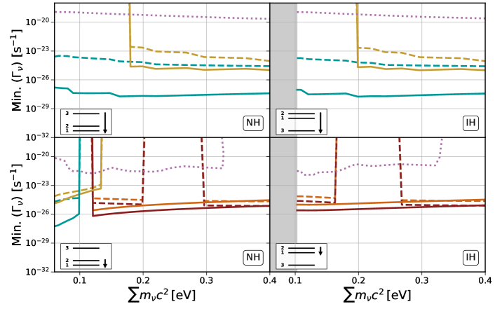
Figure 2: Forecasted 95% confidence level marginalized upper limits of $\Theta_{\nu}$ as function of the total neutrino mass from measurements for the power spectrum (dashed lines) and VID (solid lines) for all LIM surveys considered, namesly COMAP1 (orange), COMAP2 (red), CCAT-prime (dark yellow) and AtLAST (light blue). The left panels refer to the NH case, while the right ones to the IH case. In both cases we also indicate the considered transition between eigenstates. The dotted purple lines indicate the CMB limits from ref. [42, 43].

Recently, a similar situation, regarding decaying dark matter, was described in Ref. [47], where strategies to detect such decays were proposed. Here we adapt that modeling to the neutrino decay case, considering neutrino decays happening at $z<10$, and perform a Fisher-matrix analysis [69, 70, 71, 72], accounting for the uncertainity in the astrophysical model. In summary, the contribution from neutrino decays to the VID can be modeled by convoluting $\mathcal{P}_{ij}(T)$ with the astrophysical and noise VIDs: the total VID is the result of the sum of the three contributions. In turn, the contribution to the power spectrum consists of the addition of the projected power spectrum from neutrino decays to a different redshift, which introduces a strong anisotropy in the power spectrum, altering the ratio between the Legendre multipoles. For the power spectrum, we do not consider decays from the same cosmic volumes probed by the astrophysical line because they are very degenerate with astrophysical uncertainties.

We show the forecasted minimum values of $\Gamma_{ij}$ which LIM experiments will be sensitive to at the 95% confidence level, as function of the neutrino hierarchy, transition, and $\sum m_{\nu}$ in Fig. 2. We limit the minimum $\sum m_{\nu}$ at the minimum mass allowed for each hierarchy from neutrino oscillations experiments [73]. As expected from Fig. 1, COMAP and the experiments targeting CII are sensitive to the transitions between close and far mass eigenstates, respectively (with the exception of low $\sum m_{\nu}$ in the normal hierarchy).

After marginalizing over the astrophysical uncertainties of the target line as in Ref. [47], we find that for all cases considered LIM experiments can improve current cosmological bounds on the neutrino decay rate from CMB spectral distortions [42, 43] by several orders of magnitude. This shows that LIM has the potential to provide the strongest cosmological sensitivity on neutrino radiative decays. Furthermore, LIM will be competitive to the most stringent limits to date, coming from stellar cooling [39, 40, 41], as we see below.

As mentioned above, at the microscopic level radiative neutrino decays may result from an effective term in the Lagrangian like $\propto\bar{\nu}^{i}\sigma_{\alpha\beta}(\mu_{ij}+\epsilon_{ij}\gamma_{5})\nu^{j}F^{\alpha\beta}+$ hermitian conjugates [37, 14, 74], where $F^{\alpha\beta}$ is the electromagnetic field tensor, $\sigma_{\alpha\beta}$ is the Dirac gamma matrices commutator, and $\mu_{ij}$ and $\epsilon_{ij}$ are the magnetic and electric moments, respectively. For a transition (i.e., $i\neq j$), we can relate an effective electromagnetic moment $\mu^{\rm eff}_{ij}$ to the decay rate as

$$\left(\mu^{\rm eff}_{ij}\right)^{2}\simeq\frac{\Gamma_{ij}}{5\,{\rm s^{-1}}}\frac{m_{{\rm ev,}i}^{3}}{\left(m_{{\rm eV,}i}^{2}-m_{{\rm eV,}j}^{2}\right)^{3}}\mu_{\rm B}^{2}\,,$$ (5)

where $\lvert\mu^{\rm eff}_{ij}\lvert^{2}\equiv\lvert\mu_{ij}\lvert^{2}+\lvert\epsilon_{ij}\lvert^{2}$, and $\mu_{\rm B}$ is the Bohr magneton.

According to Eq. (5), the forecasted LIM sensitivity of $\Gamma_{ij}\sim 10^{-28}\,-\,10^{-25}\,{\rm s}^{-1}$ at 95% confidence level translates to $\mu_{ij}^{\rm eff}\sim 10^{-12}\,-\,10^{-8}\,(m_{i}c^{2}/{0.1\rm eV})^{3/2}\mu_{\rm B}$, while current and forecasted CMB limits are $\sim 10^{-7}\,-\,10^{-8}\mu_{\rm B}$ and $\sim 10^{-8}\,-3\times 10^{-11}\mu_{\rm B}$, respectively [43]. Note that the sensitivity to $\mu^{\rm eff}_{ij}$ depends on the mass of the original neutrino, which in turn depends on the transition, hierarchy and $\sum m_{\nu}$ considered. In turn, the most stringent direct detection limit was obtained in the Borexino experiment and is related to an effective moment accounting for all magnetic direct and transition moments: $\mu^{\rm eff}_{\nu}<2.8\times 10^{-11}\mu_{\rm B}$ at 90% confidence level [75]. Finally, astrophysical studies of stellar cooling set the strongest bounds to date: $\mu^{\rm eff}_{\nu}<4.5\times 10^{-12}\mu_{\rm B}$ at 95% confidence level [41].

This demonstrates the great potential that LIM surveys have to unveil neutrino properties: on top of having a sensitivity competitive to and in some cases even improving current strongest limits, LIM experiments may probe neutrino decays in a very different context than the rest of experiments and observations discussed above. Instead of neutrinos produced in the interior of stars, LIM will be sensitive to the cosmic neutrino background (as CMB studies are, but at very different redshifts). Moreover, the energy of the neutrinos involved in each probe also varies, which may inform about a potential energy dependence of the electromagnetic transition moments [76]. These synergies are very timely, since an enhanced magnetic moment may explain the $\sim 3\sigma$ excess observed by XENON1T [36], but the values require are close to the limits found by Borexino and in tension with stellar cooling constraints.

Finally, LIM may provide additional information about the cosmic neutrino background beyond the effect of $\sum m_{\nu}$ in the growth of perturbations: combining the information about $\sum m_{\nu}$ with the frequency of the photons produced in the decay, LIM might be the only cosmological probe sensitive to individual neutrino masses and their hierarchy [77].

The complementarity between different probes of neutrino decays will also help as a cross-check for eventual caveats or systematic uncertainties in the measurements. In the case of LIM experiments, these are the same as for the search for radiative dark matter decays, which are discussed in Ref. [47]. In summary, astrophysical uncertainties are already accounted for in our analysis, there are efficient strategies to deal with known astrophysical line interlopers [53, 54, 55, 56, 57, 58, 59, 60, 61], and galactic foregrounds are expected to be under control at the frequencies of interest. Moreover, the neutrino decay contribution to the LIM power spectrum and VID is very characteristic, and the combination of both summary statistics will not only improve the sensitivity but also the robustness of the measurement. Finally, we have assumed that the neutrino decay line is a delta function, and neglected any widening due to the neutrino velocity distributions. While this is a good approximation for the regime of interest at this stage, it is also possible to model the neutrino decay emissivity with a generic momentum distribution [43]; this will allow to adapt our analysis to neutrino production models that alter their momentum distribution [79].

The neutrino decay contribution might be confused with other exotic radiation injection such as dark matter decay. However, the shape of the neutrino power spectrum and density PDF is different. Moreover, while the contribution from dark matter decays will appear in LIM cross-correlations with galaxy clustering [46] and lensing [80], the contribution from neutrino decays will barely do, since galaxy surveys do not trace the neutrino density field.

In this letter we have proposed the use of LIM for the detection of a possible radiative decay of the cosmic neutrino background, focusing on its contribution to the LIM power spectrum and VID. We have also provided a first parametric fit of the neutrino density PDF using N-body simulations and symbolic regression, that was required to compute the contribution to the VID. Our results show that LIM have the potential to achieve sensitivities competitive to current limits, improving other cosmological probes by several orders of magnitude. The complementarity of LIM and other existing probes of neutrino decays opens exciting synergies, as well as checks for systematics, that will lead the way to new studies of neutrino properties.

Acknowledgments— JLB is supported by the Allan C. and Dorothy H. Davis Fellowship. AC acknowledges support from the the Israel Science Foundation (Grant No. 1302/19), the US-Israeli BSF (grant 2018236) and the German Israeli GIF (grant I-2524-303.7). AC acknowledges hospitality of the Max Planck Institute of Physics in Munich. FVN acknowledges funding from the WFIRST program through NNG26PJ30C and NNN12AA01C. This work was supported at Johns Hopkins by NSF Grant No. 1818899 and the Simons Foundation.

References

- [1] V. Cung and M. Yoshimura, “Electromagnetic interaction of neutrinos in gauge theories of weak interactions,” La Rivista del Nuovo Cimento 29 no. 4, (Oct., 1975) 557–564.
- [2] L. Rosenberg, “Electromagnetic interactions of neutrinos,” Phys. Rev. 129 (1963) 2786–2788.
- [3] KATRIN Collaboration, S. Mertens et al., “A novel detector system for KATRIN to search for keV-scale sterile neutrinos,” J. Phys. G 46 no. 6, (2019) 065203, arXiv:1810.06711 [physics.ins-det].
- [4] KamLAND-Zen Collaboration, A. Gando et al., “Search for Majorana Neutrinos near the Inverted Mass Hierarchy Region with KamLAND-Zen,” Phys. Rev. Lett. 117 no. 8, (2016) 082503, arXiv:1605.02889 [hep-ex]. [Addendum: Phys.Rev.Lett. 117, 109903 (2016)].
- [5] EXO-200 Collaboration, J. B. Albert et al., “Search for Majorana neutrinos with the first two years of EXO-200 data,” Nature 510 (2014) 229–234, arXiv:1402.6956 [nucl-ex].
- [6] T. Brunner and L. Winslow, “Searching for decay in 136Xe – towards the tonne-scale and beyond,” Nucl. Phys. News 27 no. 3, (2017) 14–19, arXiv:1704.01528 [hep-ex].
- [7] A. Beda, E. Demidova, A. Starostin, V. Brudanin, V. Egorov, D. Medvedev, et al., “GEMMA experiment: Three years of the search for the neutrino magnetic moment,” Phys. Part. Nucl. Lett. 7 (2010) 406–409, arXiv:0906.1926 [hep-ex].
- [8] TEXONO Collaboration, M. Deniz et al., “Measurement of Nu(e)-bar -Electron Scattering Cross-Section with a CsI(Tl) Scintillating Crystal Array at the Kuo-Sheng Nuclear Power Reactor,” Phys. Rev. D 81 (2010) 072001, arXiv:0911.1597 [hep-ex].
- [9] T2K Collaboration, K. Abe et al., “Measurement of neutrino and antineutrino oscillations by the T2K experiment including a new additional sample of interactions at the far detector,” Phys. Rev. D 96 no. 9, (2017) 092006, arXiv:1707.01048 [hep-ex]. [Erratum: Phys.Rev.D 98, 019902 (2018)].
- [10] NOvA Collaboration, P. Adamson et al., “Constraints on Oscillation Parameters from Appearance and Disappearance in NOvA,” Phys. Rev. Lett. 118 no. 23, (2017) 231801, arXiv:1703.03328 [hep-ex].
- [11] DUNE Collaboration, R. Acciarri et al., “Long-Baseline Neutrino Facility (LBNF) and Deep Underground Neutrino Experiment (DUNE): Conceptual Design Report, Volume 1: The LBNF and DUNE Projects,” arXiv:1601.05471 [physics.ins-det].
- [12] Hyper-Kamiokande Proto- Collaboration, K. Abe et al., “Physics potential of a long-baseline neutrino oscillation experiment using a J-PARC neutrino beam and Hyper-Kamiokande,” PTEP 2015 (2015) 053C02, arXiv:1502.05199 [hep-ex].
- [13] IceCube Collaboration, M. G. Aartsen et al., “Search for sterile neutrino mixing using three years of IceCube DeepCore data,” Phys. Rev. D 95 no. 11, (2017) 112002, arXiv:1702.05160 [hep-ex].
- [14] G. Raffelt, Stars as laboratories for fundamental physics: The astrophysics of neutrinos, axions, and other weakly interacting particles. 5, 1996.
- [15] B. Pontecorvo, “Neutrino Experiments and the Problem of Conservation of Leptonic Charge,” Sov. Phys. JETP 26 (1968) 984–988.
- [16] V. Gribov and B. Pontecorvo, “Neutrino astronomy and lepton charge,” Phys. Lett. B 28 (1969) 493.
- [17] P. Langacker, S. Petcov, G. Steigman, and S. Toshev, “On the Mikheev-Smirnov-Wolfenstein (MSW) Mechanism of Amplification of Neutrino Oscillations in Matter,” Nucl. Phys. B 282 (1987) 589–609.
- [18] S. M. Bilenky, J. Hosek, and S. Petcov, “On Oscillations of Neutrinos with Dirac and Majorana Masses,” Phys. Lett. B 94 (1980) 495–498.
- [19] E. K. Akhmedov, “Neutrino physics,” in ICTP Summer School in Particle Physics, pp. 103–164. 6, 1999. arXiv:hep-ph/0001264.
- [20] M. C. Gonzalez-Garcia and Y. Nir, “Neutrino Masses and Mixing: Evidence and Implications,” Rev. Mod. Phys. 75 (2003) 345–402, arXiv:hep-ph/0202058.
- [21] M. C. Gonzalez-Garcia and M. Maltoni, “Phenomenology with Massive Neutrinos,” Phys. Rept. 460 (2008) 1–129, arXiv:0704.1800 [hep-ph].
- [22] F. Boehm and P. Vogel, Physics of Massive Neutrinos. 1992.
- [23] P. B. Pal and L. Wolfenstein, “Radiative Decays of Massive Neutrinos,” Phys. Rev. D 25 (1982) 766.
- [24] S. T. Petcov, “The Processes in the Weinberg-Salam Model with Neutrino Mixing,” Sov. J. Nucl. Phys. 25 (1977) 340. [Erratum: Sov.J.Nucl.Phys. 25, 698 (1977), Erratum: Yad.Fiz. 25, 1336 (1977)].
- [25] K. Fujikawa and R. Shrock, “The Magnetic Moment of a Massive Neutrino and Neutrino Spin Rotation,” Phys. Rev. Lett. 45 (1980) 963.
- [26] N. F. Bell, M. Gorchtein, M. J. Ramsey-Musolf, P. Vogel, and P. Wang, “Model independent bounds on magnetic moments of Majorana neutrinos,” Phys. Lett. B 642 (2006) 377–383, arXiv:hep-ph/0606248.
- [27] S. Davidson, M. Gorbahn, and A. Santamaria, “From transition magnetic moments to majorana neutrino masses,” Phys. Lett. B 626 (2005) 151–160, arXiv:hep-ph/0506085.
- [28] H. Georgi and L. Randall, “Charge Conjugation and Neutrino Magnetic Moments,” Phys. Lett. B 244 (1990) 196–202.
- [29] B. W. Lee and R. E. Shrock, “Natural Suppression of Symmetry Violation in Gauge Theories: Muon - Lepton and Electron Lepton Number Nonconservation,” Phys. Rev. D 16 (1977) 1444.
- [30] R. Shrock, “Decay l0 — nu(lepton) gamma in gauge theories of weak and electromagnetic interactions,” Phys. Rev. D 9 (1974) 743–748.
- [31] M. Lindner, B. Radovčić, and J. Welter, “Revisiting Large Neutrino Magnetic Moments,” JHEP 07 (2017) 139, arXiv:1706.02555 [hep-ph].
- [32] M. Lindner, B. Radovčić, and J. Welter, “Revisiting large neutrino magnetic moments,” Journal of High Energy Physics 2017 no. 7, (Jul, 2017) . http://dx.doi.org/10.1007/JHEP07(2017)139.
- [33] O. G. Miranda, D. K. Papoulias, M. Tórtola, and J. W. F. Valle, “XENON1T signal from transition neutrino magnetic moments,” Phys. Lett. B 808 (2020) 135685, arXiv:2007.01765 [hep-ph].
- [34] K. S. Babu, S. Jana, and M. Lindner, “Large neutrino magnetic moments in the light of recent experiments,” Journal of High Energy Physics 2020 no. 10, (Oct, 2020) . http://dx.doi.org/10.1007/JHEP10(2020)040.
- [35] J. N. Bahcall, NEUTRINO ASTROPHYSICS. 1989.
- [36] XENON Collaboration, E. Aprile et al., “Excess electronic recoil events in XENON1T,” Phys. Rev. D 102 no. 7, (2020) 072004, arXiv:2006.09721 [hep-ex].
- [37] C. Giunti and A. Studenikin, “Neutrino electromagnetic interactions: a window to new physics,” Rev. Mod. Phys. 87 (2015) 531, arXiv:1403.6344 [hep-ph].
- [38] P. Vogel and J. Engel, “Neutrino electromagnetic form factors,” Phys. Rev. D 39 (Jun, 1989) 3378–3383. https://link.aps.org/doi/10.1103/PhysRevD.39.3378.
- [39] G. G. Raffelt, “New bound on neutrino dipole moments from globular-cluster stars,” Phys. Rev. Lett. 64 (Jun, 1990) 2856–2858. https://link.aps.org/doi/10.1103/PhysRevLett.64.2856.
- [40] G. Raffelt and A. Weiss, “Non-standard neutrino interactions and the evolution of red giants,” Astron. Astrophys. 264 no. 2, (Oct., 1992) 536–546.
- [41] N. Viaux, M. Catelan, P. B. Stetson, G. Raffelt, J. Redondo, A. A. R. Valcarce, and A. Weiss, “Particle-physics constraints from the globular cluster M5: Neutrino Dipole Moments,” Astron. Astrophys. 558 (2013) A12, arXiv:1308.4627 [astro-ph.SR].
- [42] A. Mirizzi, D. Montanino, and P. D. Serpico, “Revisiting cosmological bounds on radiative neutrino lifetime,” Phys. Rev. D 76 (2007) 053007, arXiv:0705.4667 [hep-ph].
- [43] J. L. Aalberts et al., “Precision constraints on radiative neutrino decay with CMB spectral distortion,” Phys. Rev. D 98 (2018) 023001, arXiv:1803.00588 [astro-ph.CO].
- [44] E. D. Kovetz et al., “Line-Intensity Mapping: 2017 Status Report,” arXiv:1709.09066 [astro-ph.CO].
- [45] E. D. Kovetz et al., “Astrophysics and Cosmology with Line-Intensity Mapping,” arXiv:1903.04496 [astro-ph.CO].
- [46] C. Creque-Sarbinowski and M. Kamionkowski, “Searching for decaying and annihilating dark matter with line intensity mapping,” Phys. Rev. D 98 no. 6, (Sep, 2018) 063524, arXiv:1806.11119 [astro-ph.CO].
- [47] J. L. Bernal, A. Caputo, and M. Kamionkowski, “Strategies to Detect Dark-Matter Decays with Line-Intensity Mapping,” arXiv:2012.00771 [astro-ph.CO].
- [48] G. Mangano, G. Miele, S. Pastor, T. Pinto, O. Pisanti, and P. D. Serpico, “Effects of non-standard neutrino-electron interactions on relic neutrino decoupling,” Nucl. Phys. B 756 (2006) 100–116, arXiv:hep-ph/0607267.
- [49] A. Lidz, S. R. Furlanetto, S. P. Oh, J. Aguirre, T.-C. Chang, O. Doré, and J. R. Pritchard, “Intensity Mapping with Carbon Monoxide Emission Lines and the Redshifted 21 cm Line,” Astrophys. J. 741 (Nov., 2011) 70, arXiv:1104.4800.
- [50] J. L. Bernal, P. C. Breysse, H. Gil-Marín, and E. D. Kovetz, “User’s guide to extracting cosmological information from line-intensity maps,” Phys. Rev. D 100 no. 12, (Dec., 2019) 123522, arXiv:1907.10067 [astro-ph.CO].
- [51] A. Lewis, A. Challinor, and A. Lasenby, “Efficient computation of CMB anisotropies in closed FRW models,” Astrophys. J. 538 (2000) 473–476, arXiv:astro-ph/9911177.
- [52] F. Villaescusa-Navarro et al., “The Quijote simulations,” Astrophys. J. Suppl. 250 no. 1, (2020) 2, arXiv:1909.05273 [astro-ph.CO].
- [53] S. P. Oh and K. J. Mack, “Foregrounds for 21-cm observations of neutral gas at high redshift,” Mon. Not. R. Astron. Soc. 346 no. 3, (Dec, 2003) 871–877, arXiv:astro-ph/0302099 [astro-ph].
- [54] X. Wang, M. Tegmark, M. G. Santos, and L. Knox, “21 cm Tomography with Foregrounds,” Astrophys. J. 650 no. 2, (Oct, 2006) 529–537, arXiv:astro-ph/0501081 [astro-ph].
- [55] A. Liu and M. Tegmark, “A method for 21 cm power spectrum estimation in the presence of foregrounds,” Phys. Rev. D 83 no. 10, (May, 2011) 103006, arXiv:1103.0281 [astro-ph.CO].
- [56] P. C. Breysse, E. D. Kovetz, and M. Kamionkowski, “Masking line foregrounds in intensity-mapping surveys,” Mon. Not. R. Astron. Soc. 452 no. 4, (Oct, 2015) 3408–3418, arXiv:1503.05202 [astro-ph.CO].
- [57] A. Lidz and J. Taylor, “On Removing Interloper Contamination from Intensity Mapping Power Spectrum Measurements,” Astrophys. J. 825 no. 2, (July, 2016) 143, arXiv:1604.05737 [astro-ph.CO].
- [58] G. Sun, L. Moncelsi, M. P. Viero, M. B. Silva, J. Bock, C. M. Bradford, et al., “A Foreground Masking Strategy for [C II] Intensity Mapping Experiments Using Galaxies Selected by Stellar Mass and Redshift,” Astrophys. J. 856 no. 2, (Apr, 2018) 107, arXiv:1610.10095 [astro-ph.GA].
- [59] Y.-T. Cheng, T.-C. Chang, J. Bock, C. M. Bradford, and A. Cooray, “Spectral Line De-confusion in an Intensity Mapping Survey,” Astrophys. J. 832 no. 2, (Dec, 2016) 165, arXiv:1604.07833 [astro-ph.CO].
- [60] Y.-T. Cheng, T.-C. Chang, and J. J. Bock, “Phase-space Spectral Line Deconfusion in Intensity Mapping,” Astrophys. J. 901 no. 2, (Oct., 2020) 142, arXiv:2005.05341 [astro-ph.CO].
- [61] Y. Gong, X. Chen, and A. Cooray, “Cosmological Constraints from Line Intensity Mapping with Interlopers,” Astrophys. J. 894 no. 2, (May, 2020) 152, arXiv:2001.10792 [astro-ph.CO].
- [62] K. Cleary, M.-A. Bigot-Sazy, D. Chung, et al., “The CO Mapping Array Pathfinder (COMAP),” AAS Meeting Abstracts #227 227 (Jan., 2016) 426.06.
- [63] S. K. Choi et al., “Sensitivity of the Prime-Cam Instrument on the CCAT-Prime Telescope,” Journal of Low Temperature Physics 199 no. 3-4, (Mar., 2020) 1089–1097, arXiv:1908.10451 [astro-ph.IM].
- [64] P. D. Klaassen, T. K. Mroczkowski, C. Cicone, E. Hatziminaoglou, S. Sartori, C. De Breuck, et al., “The Atacama Large Aperture Submillimeter Telescope (AtLAST),” in Society of Photo-Optical Instrumentation Engineers (SPIE) Conference Series, vol. 11445 of Society of Photo-Optical Instrumentation Engineers (SPIE) Conference Series, p. 114452F. Dec., 2020. arXiv:2011.07974 [astro-ph.IM].
- [65] T. Y. Li, R. H. Wechsler, K. Devaraj, and S. E. Church, “Connecting CO Intensity Mapping to Molecular Gas and Star Formation in the Epoch of Galaxy Assembly,” Astrophys. J. 817 (Feb., 2016) 169, arXiv:1503.08833 [astro-ph.CO].
- [66] M. Silva, M. G. Santos, A. Cooray, and Y. Gong, “Prospects for Detecting C II Emission during the Epoch of Reionization,” Astrophys. J. 806 no. 2, (Jun, 2015) 209, arXiv:1410.4808 [astro-ph.GA].
- [67] P. C. Breysse, E. D. Kovetz, P. S. Behroozi, L. Dai, and M. Kamionkowski, “Insights from probability distribution functions of intensity maps,” Mon. Not. R. Astron. Soc. 467 (May, 2017) 2996–3010, arXiv:1609.01728 [astro-ph.CO].
- [68] Planck Collaboration, N. Aghanim, Y. Akrami, M. Ashdown, J. Aumont, C. Baccigalupi, et al., “Planck 2018 results: VI. Cosmological parameters,” Astronomy and Astrophysics 641 (Sep, 2020) A6, arXiv:1807.06209. https://doi.org/10.1051/0004-6361/201833910.
- [69] R. A. Fisher, “The Fiducial Argument in Statistical Inference,” Annals Eugen. 6 (1935) 391–398.
- [70] G. Jungman, M. Kamionkowski, A. Kosowsky, and D. N. Spergel, “Weighing the universe with the cosmic microwave background,” Phys. Rev. Lett. 76 (1996) 1007–1010, arXiv:astro-ph/9507080.
- [71] G. Jungman, M. Kamionkowski, A. Kosowsky, and D. N. Spergel, “Cosmological parameter determination with microwave background maps,” Phys. Rev. D 54 (1996) 1332–1344, arXiv:astro-ph/9512139.
- [72] M. Tegmark, A. N. Taylor, and A. F. Heavens, “Karhunen-Loève Eigenvalue Problems in Cosmology: How Should We Tackle Large Data Sets?,” Astrophys. J. 480 (May, 1997) 22–35, astro-ph/9603021.
- [73] I. Esteban, M. Gonzalez-Garcia, A. Hernandez-Cabezudo, M. Maltoni, and T. Schwetz, “Global analysis of three-flavour neutrino oscillations: synergies and tensions in the determination of , , and the mass ordering,” JHEP 01 (2019) 106, arXiv:1811.05487 [hep-ph].
- [74] V. Brdar, A. Greljo, J. Kopp, and T. Opferkuch, “The Neutrino Magnetic Moment Portal: Cosmology, Astrophysics, and Direct Detection,” JCAP 01 (2021) 039, arXiv:2007.15563 [hep-ph].
- [75] Borexino Collaboration, M. Agostini et al., “Limiting neutrino magnetic moments with Borexino Phase-II solar neutrino data,” Phys. Rev. D 96 no. 9, (2017) 091103, arXiv:1707.09355 [hep-ex].
- [76] J. M. Frere, R. B. Nevzorov, and M. I. Vysotsky, “Stimulated neutrino conversion and bounds on neutrino magnetic moments,” Phys. Lett. B 394 (1997) 127–131, arXiv:hep-ph/9608266.
- [77] M. Archidiacono, S. Hannestad, and J. Lesgourgues, “What will it take to measure individual neutrino mass states using cosmology?,” JCAP 2020 no. 9, (Sept., 2020) 021, arXiv:2003.03354 [astro-ph.CO].
- [78] H. T. Ihle, D. Chung, G. Stein, M. Alvarez, J. R. Bond, P. C. Breysse, et al., “Joint Power Spectrum and Voxel Intensity Distribution Forecast on the CO Luminosity Function with COMAP,” Astrophys. J. 871 (Jan, 2019) 75, arXiv:1808.07487 [astro-ph.CO].
- [79] A. Merle and M. Totzauer, “keV Sterile Neutrino Dark Matter from Singlet Scalar Decays: Basic Concepts and Subtle Features,” JCAP 06 (2015) 011, arXiv:1502.01011 [hep-ph].
- [80] M. Shirasaki, “Searching for eV-mass Axion-like Particles with Cross Correlations between Line Intensity and Weak Lensing Maps,” arXiv e-prints (Jan., 2021) arXiv:2102.00580, arXiv:2102.00580 [astro-ph.CO].