Extracting the Unknown from Long Math Problems
Abstract
In problem solving, understanding the problem that one seeks to solve is an essential initial step. In this paper, we propose computational methods for facilitating problem understanding through the task of recognizing the unknown in specifications of long Math problems. We focus on the topic of Probability. Our experimental results show that learning models yield strong results on the task — a promising first step towards human interpretable, modular approaches to understanding long Math problems.
1 Introduction
“It is foolish to answer a question that you do not understand. It is sad to work for an end that you do not desire— George Polya Polya (1957). According to Mathematician Polya’s famous problem solving heuristics, asking general common sense questions about the problem facilitates problem understanding. One such question is “What is the unknown?” Polya (1957). The unknown of a given problem is what the problem requires to be worked out and solved. In this paper, we propose computational models for extracting the unknown from problem specifications.
In online tutorial communities, it is not uncommon to find problems that include questions like “what is the solution I am looking for?”111https://stats.stackexchange.com/questions/66766/. Automated hints such as help with identifying the unknown, could provide timely support to self-directed learners Guglielmino (1978); Houle (1988); Hiemstra (1994). Furthermore, information about the unknown can be used as a feature in other tasks that can enhance self-directed learning, such as similar-question retrieval Lei et al. (2016), and question-answer matching Shen et al. (2017), as well as in models for automated problem solving Sachan et al. (2018).
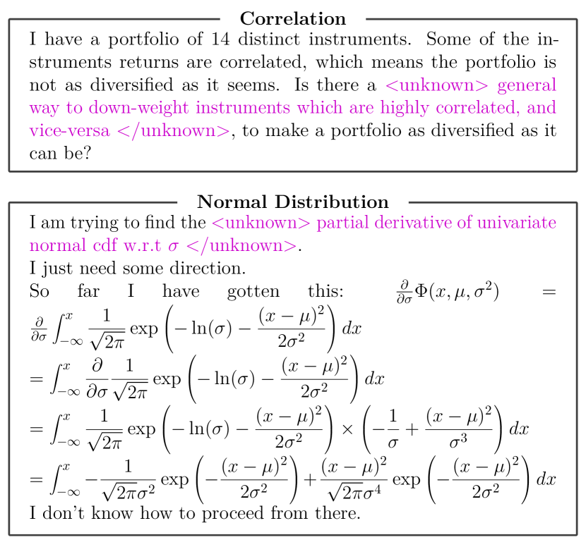
The unknown is general, it not restricted to problems about a particular subject-matter. The problem can be algebraic, geometric, mathematical or nonmathematical Polya (1957). In this paper, we focus on the topic of Probability as a case study. To facilitate model training, we created a dataset, ProbUNK, containing Probability problems labeled with their unknown(s). Figure 1 shows example problems from ProbUNK.
Prior Work.
Our work is related to question understanding, and modular approaches to question answering that advocate decomposing questions into smaller ones Andreas et al. (2016); Iyyer et al. (2017); Gupta and Lewis (2018); Talmor and Berant (2018); Huang et al. (2018); Guo et al. (2019); Min et al. (2019); Wolfson et al. (2020). However, question decomposition in prior work is aimed at enhancing model performance, and is generally not human friendly. Notions of interpretability are provided through attention modules Andreas et al. (2016), or explicit meaning representations such as first-order logic Sachan et al. (2018), or custom semantic parsing formalisms Amini et al. (2019); Wolfson et al. (2020). In contrast, our goal is to produce output that can be used by humans, and potentially by models too. Additionally, questions in most prior work are short, containing just a single sentence. We target longer multi-sentence problems.
2 Dataset
Background Knowledge on Probability.
As background knowledge, we collected information about probability concepts. We define a probability concept as a term that is formally defined in the first five chapters of Wasserman (2013), and appears in the index at the end of that book. This produced concepts. For example, ‘Poisson Distribution’, ‘Correlation’, see appendix for full list. We augment each concept with content from DeGroot and Schervish (2012). On average per concept, we collected definitions worked-out examples, and unworked-out examples, from both books.
| Train | Dev | Test | |
| Problems | 904 | 110 | 157 |
| Answers | 904 | 110 | 157 |
| Total | 1,808 | 220 | 314 |
StackExchange Probability Problems.
We obtained the data dump from stats.stackexchange, containing Statistics problems. Each problem is labeled with relevant concept tags. We discarded all programming-related problems, tagged with: ‘Matlab’ and ‘R’, resulting in problems. We also pruned concept tags outside of the background concepts. To avoid overly complex problems, those with tags were pruned. Lastly, we only kept problems for which there is an ‘accepted answer’ from the forum. Overall after pre-processing, there were remaining problems, spanning 11 Probability concepts, along with their answers. Table 1 shows the train/dev/test split222Breakdown of problems by concept is in the appendix..
| Dev | Test | Training | ||
| Method | F1 | F1 | time | |
| 1. | MaxEnt | 04m32s | ||
| 2. | MLP | 06m24s | ||
| 3. | LSTM | 28m41s | ||
| 4. | GRU | 25m36s | ||
| 5. | CNN | 0.754 | 0.727 | 03m39s |
| 6. | Prototypical Nets(*) | 0.787 | 0.782 | 03m21s |
Concept Classification.
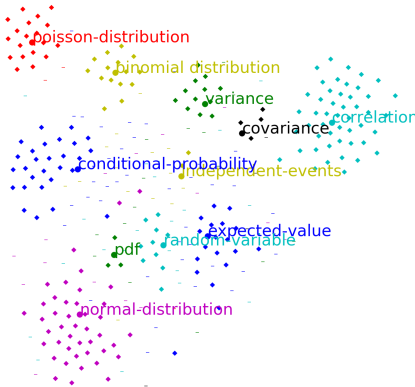
Given the size of our dataset, our setting falls within the limited labeled data regime Palatucci et al. (2009); Sachan et al. (2018). To investigate whether our dataset is sufficient for training models that generalize, we considered a simple task: classifying problems by their concepts. This is a multi-label333 of the problems in our dataset span concepts. classification task. We used a pretrained transformer, BERT Devlin et al. (2019), to obtain contextualised word embeddings, and then trained444Training setup details are in the appendix. various models. The results are shown in Table 2. For the MaxEnt model (a logistic regression classifier), and the multi-layer perceptron, MLP, problem representations were obtained by average pooling of the word embeddings. From initial experiments we found that using the CLS token representation, instead of average pooling, degrades performance. A Convolutional Neural Network (CNN) text classifier, kernel sizes: ,,, , each with kernels, has the strongest performance on the full problem, F1 on test data. We also implemented Prototypical Networks Snell et al. (2017), an approach designed for limited labeled data settings. We used a CNN (same settings as above) as the base model for learning prototypical vector representations. We evaluated the Prototypical Network on problems that are about a single concept, of dev, and of test data, and it produced strong results, F1 . Visualizing the learned prototypes and prototypical problems, Figure 2 shows that the learned representations are meaningful. For instance, prototypical problems of type Poisson Distribution are closest to the prototypical vector of that concept. This is not trivially expected because there are many prototypical vectors for a concept, which are generated from different support vectors (refer to Snell et al. (2017) for details), and we randomly picked one prototypical vector for each concept.
Overall, both the quantitative results in Table 2, and the qualitative results in Figure 2, show that our dataset is adequate for learning meaningful representations, when using pre-trained contextual embeddings.
Unknown Annotation.
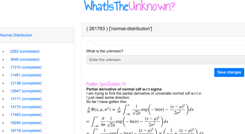
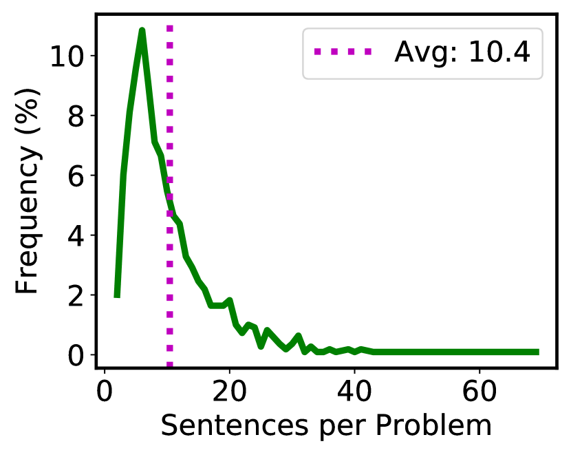
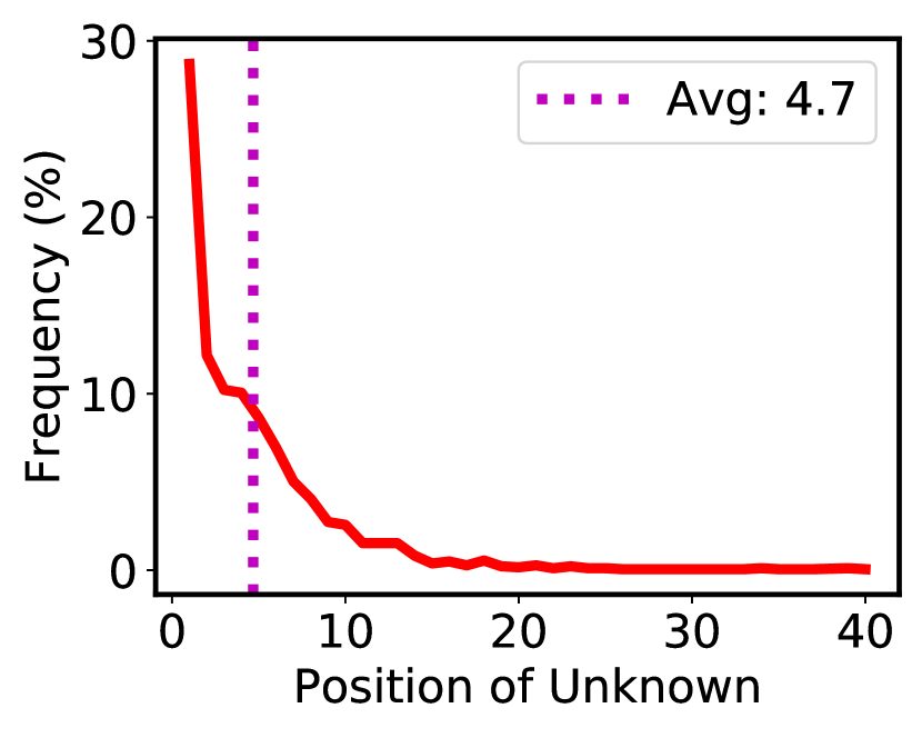
To collect labeled data, we assume the unknown is a contiguous sequence of tokens in the problem specification. We implemented a simple labeling tool, shown in Figure 3. A problem can have multiple unknowns, each unknown is entered separately. In total, problems were annotated. Problems whose unknowns were deemed ‘unclear’ were few: , , and for train, dev, test, respectively. On average the unknown(s) is (are) spread across . Figures 4(a) and 4(b) show distributions of sentences per problem, and position of the unknown.
| DEV | TEST | Training | ||
| Method | F1 | F1 | time | |
| 1. | Majority | n/a | ||
| 2. | st Sentence | n/a | ||
| 3. | nd Sentence | n/a | ||
| 4. | Last Sentence | n/a | ||
| 5. | MaxEnt | 02m19s | ||
| 6. | MLP | 03m06s | ||
| 7. | CNN | 10m31s | ||
| 8. | CNN_NoContext | 09m10s | ||
| 9. | CNN + Graph | 0.780 | 16m42s | |
| 10. | CNN + Graph + LSTM | 19m48s | ||
| 11. | CNN + Graph + GRU | 18m44s |
3 Approach
Given a sentence, our goal is to predict if it contains a sequence of words that describe the unknown, , or not, . Alternative formulation is to treat the problem a sequence labeling task. However, in this initial work, the labeled data we obtained is at the sentence level. With the right granularity of labeled data, our task be cast as a sequence labeling task.
Input, Prediction, and Loss.
As input, a problem specification, , and the -th sentence, , are presented to a model. A context vector, , is generated from , and a sentence vector, is generated from . The two vectors are concatenated to compute as follows:
where is the sigmoid function, and are learned via the cross entropy loss
.
Context Vectors.
To compute the context vector, , we consider different approaches.
BoW context: is obtained by average pooling BERT embeddings of the tokens of .
CNN Context: is generated by applying a CNN to .
GCN Context: is generated from a Graph Convolutional Network (GCN) Bruna et al. (2014); Defferrard et al. ; Kipf and Welling (2017). Given a graph with nodes, the input to a GCN is a feature matrix where a row contains the initial representation, of a node . To compute a node’s hidden representation, , a single graph convolution layer uses the node’s neighbors ,:
, is a non-linear activation function, and are learned. We apply the GCN recurrence for steps. At every step, node representations are re-computed using the representation of the nodes’s neighbors from the previous step, see Kipf and Welling (2017) for details.
The goal is to use the graph to learn the kinds of unknowns that pertain to different concepts, as well as to exploit relationships between problems and answers. We construct a graph with three types of nodes: concept, problem; and answer nodes. We have edge types: problem-has-type (between problems and concepts); problems-has-answer (between problems and answers); and same-section-as, mentioned-in-before-chapters, same-chapter-as (all three between concepts). We use the concept hierarchy derived from the ordering of concepts in Wasserman (2013) to obtain the last three relationships. Our graph consists of nodes, edges, and initial node features obtained from BERT embeddings. Node features are from average pooling the embeddings. For the concept nodes, the pooled tokens are taken from the concept definitions. The task for learning node representations is predicting the problem-has-type links.
| 1. | How could one derive joint pdf of ? |
| 2. | How to derive the formula of the t-test of the correlation coefficient |
| 3. | How do you calculate the expected value of ? |
| 4. | I want to calculate |
| 5. | What is the probability that the time between trains arriving is 6 minutes or less? |
| 6. | What is the probability that people in the group are fatigued |
| 7. | How do we prove that is not a bivariate normal? |
| 8. | I want to prove that the output of is independent of any input distribution. |
4 Experimental Evaluation
We conducted experiments to evaluate performance of various models on the task of extracting the unknown. All experiments are based on the train/dev/test split in Table 1. Training and computing infrastructure details are in the appendix.
Methods under Comparison.
Next to each learning method is the number of parameters. 1) Majority. Assigns the most common label, to every sentence. 2-4) -th Sentence assigns to the -th sentence, and to all others. 5) MaxEn (). Uses BoW for the context vector, , and the sentence vector . 6) MLP (). Uses the same and as method (5). 7) CNN (). A CNN generates both , and . 8) CNN_NoContext (). Same as (7) but is omitted, thus the CNN only encodes the sentence. 9. CNN+Graph (). Concatenates CNN and GCN contexts to get , whereas is obtained from just the CNN. 10) CNN+Graph+LSTM (). is as in (9), and is generated by an LSTM. 11) CNN+Graph+GRU (). Same as (10) but is generated by a GRU.
Results.
Table 3 shows our main results. Among non learning baselines, the st sentence (2) baseline achieves the best performance, F1 is on the test data. A CNN (7), well-understood to be a strong text classifier, achieves F1 of on the test data. We see the context vector is important as CNN_NoContext (8) has lower performance than (7). Incorporating graph structure, CNN+Graph (9), yields F1 of . CNN+Graph+LSTM/GRU (10-11) both yield poor results. This is likely due to the size of our dataset given that these methods have about twice as many parameters as the other methods, for example, CNN+Graph+LSTM has parameters vs. CNN+Graph with .
What cues are the methods relying on to achieve strong performance on this task? We sampled some sentences from data, a few of which are shown in Table 4. It is clear that unambiguous cues for our task are indeed in the sentences, such as “derive”, “calculate”, “what is the probability that ”, and “prove that ”. In addition to these sentence cues, our results, (7) vs. (8) and (9) in Table 4 show that there are also useful signals in the context.
5 Conclusions and Future Work
Our new task, dataset, and results are only initial steps, and pave the way for future work. Beyond “what is the unknown?”, we can develop models that ask other general common sense questions that can support the problem solving process. Polya (1957) presents a list of more such questions. These questions are general, future work includes working on problems from topics other than Probability. Additionally, future work can study who this line of work can benefit from well-studied aspects of knowledge harvesting and representation Nakashole et al. (2010); Theobald et al. (2010); Nakashole et al. (2012); Nakashole (2012); Kumar et al. (2017).
References
- Amini et al. (2019) Aida Amini, Saadia Gabriel, Peter Lin, Rik Koncel-Kedziorski, Yejin Choi, and Hannaneh Hajishirzi. 2019. Mathqa: Towards interpretable math word problem solving with operation-based formalisms. arXiv preprint arXiv:1905.13319.
- Andreas et al. (2016) Jacob Andreas, Marcus Rohrbach, Trevor Darrell, and Dan Klein. 2016. Learning to compose neural networks for question answering. In NAACL HLT, pages 1545–1554. The Association for Computational Linguistics.
- Bruna et al. (2014) Joan Bruna, Wojciech Zaremba, Arthur Szlam, and Yann LeCun. 2014. Spectral networks and locally connected networks on graphs. In ICLR.
- (4) Michaël Defferrard, Xavier Bresson, and Pierre Vandergheynst. Convolutional neural networks on graphs with fast localized spectral filtering.
- DeGroot and Schervish (2012) Morris H DeGroot and Mark J Schervish. 2012. Probability and statistics. Pearson Education.
- Devlin et al. (2019) Jacob Devlin, Ming-Wei Chang, Kenton Lee, and Kristina Toutanova. 2019. BERT: pre-training of deep bidirectional transformers for language understanding. In NAACL-HLT, pages 4171–4186.
- Guglielmino (1978) Lucy M Guglielmino. 1978. Development of the self-directed learning readiness scale. Ph.D. thesis, ProQuest Information & Learning.
- Guo et al. (2019) Jiaqi Guo, Zecheng Zhan, Yan Gao, Yan Xiao, Jian-Guang Lou, Ting Liu, and Dongmei Zhang. 2019. Towards complex text-to-sql in cross-domain database with intermediate representation. In ACL, pages 4524–4535.
- Gupta and Lewis (2018) Nitish Gupta and Mike Lewis. 2018. Neural compositional denotational semantics for question answering. In EMNLP, pages 2152–2161.
- Hiemstra (1994) R Hiemstra. 1994. Self-directed learning. In. T. Husen & TN Postlethwaite (Ed.). The International Encyclopedia of Education (2nd). Oxford: Pergamon Press.
- Horwitz et al. (1986) Elaine K Horwitz, Michael B Horwitz, and Joann Cope. 1986. Foreign language classroom anxiety. The Modern language journal, 70(2):125–132.
- Houle (1988) Cyril O Houle. 1988. The inquiring mind: A study of the adult who continues to learn.
- Huang et al. (2018) Danqing Huang, Jin-Ge Yao, Chin-Yew Lin, Qingyu Zhou, and Jian Yin. 2018. Using intermediate representations to solve math word problems. In ACL, pages 419–428.
- Iyyer et al. (2017) Mohit Iyyer, Wen-tau Yih, and Ming-Wei Chang. 2017. Search-based neural structured learning for sequential question answering. In ACL, pages 1821–1831.
- Kipf and Welling (2017) Thomas N. Kipf and Max Welling. 2017. Semi-supervised classification with graph convolutional networks. In ICLR.
- Kumar et al. (2017) Anurag Kumar, Bhiksha Raj, and Ndapandula Nakashole. 2017. Discovering sound concepts and acoustic relations in text. In Acoustics, Speech and Signal Processing (ICASSP), 2017 IEEE International Conference on, pages 631–635. IEEE.
- Lei et al. (2016) Tao Lei, Hrishikesh Joshi, Regina Barzilay, Tommi S. Jaakkola, Kateryna Tymoshenko, Alessandro Moschitti, and Lluís Màrquez. 2016. Semi-supervised question retrieval with gated convolutions. In NAACL HLT, pages 1279–1289.
- Min et al. (2019) Sewon Min, Victor Zhong, Luke Zettlemoyer, and Hannaneh Hajishirzi. 2019. Multi-hop reading comprehension through question decomposition and rescoring. In ACL, pages 6097–6109.
- Nakashole et al. (2012) Ndapandula Nakashole, Mauro Sozio, Fabian M. Suchanek, and Martin Theobald. 2012. Query-time reasoning in uncertain RDF knowledge bases with soft and hard rules. In Proceedings of the Second International Workshop on Searching and Integrating New Web Data Sources, Istanbul, Turkey, August 31, 2012, volume 884, pages 15–20.
- Nakashole et al. (2010) Ndapandula Nakashole, Martin Theobald, and Gerhard Weikum. 2010. Find your advisor: Robust knowledge gathering from the web. In Proceedings of the 13th International Workshop on the Web and Databases 2010, WebDB 2010, Indianapolis, Indiana, USA, June 6, 2010. ACM.
- Nakashole (2012) Ndapandula T Nakashole. 2012. Automatic extraction of facts, relations, and entities for web-scale knowledge base population.
- Palatucci et al. (2009) Mark Palatucci, Dean Pomerleau, Geoffrey E. Hinton, and Tom M. Mitchell. 2009. Zero-shot learning with semantic output codes. In NIPS, pages 1410–1418.
- Polya (1957) George Polya. 1957. How to solve it. Doubleday, Garden City, NY.
- Qu et al. (2012) Bo Qu, Gao Cong, Cuiping Li, Aixin Sun, and Hong Chen. 2012. An evaluation of classification models for question topic categorization. J. Assoc. Inf. Sci. Technol., 63(5):889–903.
- Sachan et al. (2018) Mrinmaya Sachan, Kumar Avinava Dubey, Tom M. Mitchell, Dan Roth, and Eric P. Xing. 2018. Learning pipelines with limited data and domain knowledge: A study in parsing physics problems. In NeurIPS, pages 140–151.
- Shen et al. (2017) Yikang Shen, Wenge Rong, Nan Jiang, Baolin Peng, Jie Tang, and Zhang Xiong. 2017. Word embedding based correlation model for question/answer matching. In Proceedings of AAAI, pages 3511–3517.
- Snell et al. (2017) Jake Snell, Kevin Swersky, and Richard Zemel. 2017. Prototypical networks for few-shot learning. In NeurIPS, pages 4077–4087.
- Talmor and Berant (2018) Alon Talmor and Jonathan Berant. 2018. The web as a knowledge-base for answering complex questions. In NAACL-HLT, pages 641–651.
- Theobald et al. (2010) Martin Theobald, Mauro Sozio, Fabian Suchanek, and Ndapandula Nakashole. 2010. Urdf: Efficient reasoning in uncertain rdf knowledge bases with soft and hard rules.
- Wasserman (2013) Larry Wasserman. 2013. All of statistics: a concise course in statistical inference. Springer Science & Business Media.
- Wolfson et al. (2020) Tomer Wolfson, Mor Geva, Ankit Gupta, Yoav Goldberg, Matt Gardner, Daniel Deutch, and Jonathan Berant. 2020. Break it down: A question understanding benchmark. Trans. Assoc. Comput. Linguistics, 8:183–198.
6 Dataset
6.1 Prototypes Visualization Further Details
We defined prototypical examples as those whose closest prototypical vector is almost always (in of the cases) that of the gold truth concept, regardless of the choice of support problems used to generate the prototypical vector. We then randomly picked one of the prototypical vectors, plotted it, and a few of the prototypical example problems.
6.2 Background Knowledge Concepts
The 69 Background knowledge concepts collected in our dataset are shown in Table 5. Definitions, along with worked out example for each concept are in the dataset.
6.3 Stats.StackExchange Preprocessing
Excluded and ignored tags are shown in Table 7. If the tag is excluded, we remove from our dataset problems with this tag. If a tag is ignored, we can keep the problem but only if it has other tags besides an ignored tags.
6.4 Train/Dev/Test by Concept
Train/Dev/Test split of our dataset listing the number of problems in each partition per concept is shown in Table 6.
6.5 Concept Classification Training Details
Implementation.
In our implementation, we used the Pytorch Library.
Computing Infrastructure.
OS: 16.04.1-Ubuntu/ x86_64.
GPU: GeForce GTX 1080 Ti with 12 GB of memory.
Evaluation Metrics.
Evaluation metric is Macro f1_score: We used the implementation in sklearn. In python, the code is: ‘from sklearn.metrics import f1_score’
Training and Method Details.
We use the ADAM optimizer, and dropout 0. Word embeddings are initialized with pretrained dimensional BERT embeddings. The MLP has hidden layers, and the dimensionality of hidden states is . The LSTM is a one layer bidirectional LSTM, with hidden dimensions . Concatenating backward and forward outputs of BiLSTM generates LSTM output vector of size . The GRU is a one layer bidirectional GRU, with hidden dimensions of . Concatenating backward and forward outputs of BiGRU generates GRU output vector of size .
Table 8 shows performance on the dev set over 11 seeds are used.
Parameter details for the methods for concept classification are in Table 9.
|
|
| Concept | Train | #. Dev | Test |
| The Binomial Distribution | 78 | 8 | 13 |
| Conditional Probability | 135 | 16 | 25 |
| Correlation | 141 | 15 | 26 |
| Covariance | 64 | 8 | 7 |
| Expected Value | 134 | 16 | 21 |
| Independent Events | 73 | 7 | 8 |
| Normal Distribution | 193 | 22 | 29 |
| Probability Density Function | 49 | 4 | 3 |
| The Poisson Distribution | 58 | 6 | 9 |
| Random Variable | 133 | 20 | 26 |
| Variance | 103 | 14 | 17 |
| Total | 1,161 | 136 | 184 |
| #. Unique Problems | 904 | 110 | 157 |
| #. Unique Answers | 904 | 110 | 157 |
| Total | 1808 | 220 | 314 |
| TAG | Excluded/Ignored | REASON |
| Matlab | Excluded | programming problems |
| R | Excluded | programming problems |
| Probability | Ignore | Too Generic |
| Mathematical-statistics | Ignore | Too Generic |
| Meta-analysis | Ignore | Too Generic |
| Hypothesis-testing’ | Ignore | Too Generic |
| Distributions | Ignore | Too Generic |
| Self-study | Ignore | Too Generic |
| Intuition | Ignore | Too Generic |
| Definition | Ignore | Too Generic |
| Dev | ||
| Method | F1 | |
| 1. | MaxEnt | |
| 2. | MLP | |
| 3. | LSTM | |
| 4. | GRU | |
| 5. | CNN |
| MaxEnt | #. Parameters | 8,459 |
| Epochs (bounds) | [1-300] | |
| Epochs (best) | 300 | |
| Number of epochs search trials | 31 | |
| Choosing hyperparameter values | uniform (1, 10, 20, 30, … | |
| Seed | 3 | |
| MLP | #. Parameters | 924,683 |
| Epochs (bounds) | [1-300] | |
| Epochs (best) | 300 | |
| Number of epochs search trials | 31 | |
| Method of choosing epoch values | uniform: 1, 10, 20, 30, … | |
| Seed | 1 | |
| LSTM | #. Parameters | 4,469,771 |
| Epochs (bounds) | [1-300] | |
| Epochs (best) | 300 | |
| Number of epochs search trials | 31 | |
| Method of choosing epoch values | uniform: 1, 10, 20, 30, … | |
| Seed | 2 | |
| GRU | #. Parameters | 3,583,499 |
| Epochs (bounds) | [1-300] | |
| Epochs (best) | 300 | |
| Number of epochs search trials | 31 | |
| Method of choosing epoch values | uniform: 1, 10, 20, 30, … | |
| Seed | 2 | |
| CNN | #. Parameters | 3,138,829 |
| Epochs (bounds) | [1-300] | |
| Epochs (best) | 20 | |
| Number of epochs search trials | 31 | |
| Method of choosing epoch values | uniform: 1, 10, 20, 30, … | |
| Seed | 10000 | |
| Filter Sizes (bounds) | combinations of [1,2,3,4,5,6] | |
| Filter Sizes (best) | [3,4,5,6] | |
| Method of choosing Filter Sizes | manual | |
| Filters (bounds) | [50-300] | |
| Filters (best) | [192] | |
| Method of choosing Filters | manual | |
| Prototypical Networks | #. Parameters | 2,214,146 |
| Episodes (bounds) | [10-200] | |
| Episodes (best) | 100 | |
| Method of choosing episode values | uniform | |
| Support size | 10 | |
| Query size | 15 |
7 Experimental Evaluation
Computing Infrastructure.
Operating System: 16.04.1-Ubuntu/ x86_64.
GPU: GeForce GTX 1080 Ti with 12 GB of memory.
Evaluation Metrics.
Evaluation metric is Macro f1_score: We used the implementation in sklearn. In python, the code is: ‘from sklearn.metrics import f1_score’
Training and Method details
The GCN input features are -dimensional, and its hidden states are dimensional, and the number of convolutional layers is .
We use the ADAM optimizer, and dropout . Word embeddings are initialized with pretrained dimensional BERT embeddings. The MLP has hidden layers, and the dimensionalities of hidden states is . The LSTM is a one layer bidirectional LSTM, with hidden dimensions . The GRU is a one layer bidirectional GRU.
Parameter details for the methods for unknown extraction are in Table 10.
| MaxEnt | #. Parameters | 1,537 |
| Epochs (bounds) | [1-100] | |
| Epochs (best) | 30 | |
| Number of epochs search trials | 11 | |
| Choosing epochs values | uniform (1, 10, 20, 30, … | |
| Seed | 3 | |
| MLP | #. Parameters | 1,312,769 |
| Epochs (bounds) | [1-50] | |
| Epochs (best) | 30 | |
| Number of epochs search trials | 6 | |
| Choosing epochs values | uniform (1, 10, 20, 30, … | |
| Seed | 10 | |
| CNN | #. Parameters | 1,414,275 |
| Epochs (bounds) | [1-100] | |
| Epochs (best) | 20 | |
| Number of epochs search trials | 6 | |
| Choosing epochs values | uniform (1, 10, 20, 30, … | |
| Seed | 4 | |
| Filter Sizes (bounds) | combinations of [1,2,3,4,5,6] | |
| Filter Sizes (best) | [1,2] | |
| Method of choosing Filter Sizes | manual | |
| Filters (bounds) | [50-300] | |
| Filters (best) | [192] | |
| Method of choosing Filters | manual | |
| CNN_NoContext | #. Parameters | 1,166,467 |
| Epochs (bounds) | [1-50] | |
| Epochs (best) | 30 | |
| Number of epochs search trials | 6 | |
| Seed | 0 | |
| CNN+Graph | #. Parameters | 1,502,386 |
| Epochs (bounds) | [1-50] | |
| Epochs (best) | 30 | |
| Number of epochs search trials | 6 | |
| Seed | 0 | |
| GCN layers | 3 | |
| GCN hidden state dimensionality | ||
| CNN+Graph+LSTM | #. Parameters | 2,980,018 |
| Epochs (bounds) | [1-50] | |
| Epochs (best) | 30 | |
| Number of epochs search trials | 6 | |
| Seed | 10000 | |
| CNN+Graph+GRU | #. Parameters | 2,610,610 |
| Epochs (bounds) | [1-50] | |
| Epochs (best) | 30 | |
| Number of epochs search trials | 6 | |
| Seed | 10 |