Scale dependence and cross-scale transfer of kinetic energy in compressible hydrodynamic turbulence at moderate Reynolds numbers

Abstract

We investigate properties of the scale dependence and cross-scale transfer of kinetic energy in compressible three-dimensional hydrodynamic turbulence, by means of two direct numerical simulations of decaying turbulence with initial Mach numbers $M=1/3$ and $M=1$, and with moderate Reynolds numbers, $R_{\lambda}\sim 100$. The turbulent dynamics is analyzed using compressible and incompressible versions of the dynamic spectral transfer (ST) and the Kármán-Howarth-Monin (KHM) equations. We find that the nonlinear coupling leads to a flux of the kinetic energy to small scales where it is dissipated; at the same time, the reversible pressure-dilatation mechanism causes oscillatory exchanges between the kinetic and internal energies with an average zero net energy transfer. While the incompressible KHM and ST equations are not generally valid in the simulations, their compressible counterparts are well satisfied and describe, in a quantitatively similar way, the decay of the kinetic energy on large scales, the cross-scale energy transfer/cascade, the pressure dilatation, and the dissipation. There exists a simple relationship between the KHM and ST results through the inverse proportionality between the wave vector $k$ and the spatial separation length $l$ as $kl\simeq\sqrt{3}$. For a given time the dissipation and pressure-dilatation terms are strong on large scales in the KHM approach whereas the ST terms become dominant on small scales; this is owing to the complementary cumulative behavior of the two methods. The effect of pressure dilatation is weak when averaged over a period of its oscillations and may lead to a transfer of the kinetic energy from large to small scales without a net exchange between the kinetic and internal energies. Our results suggest that for large-enough systems there exists an inertial range for the kinetic energy cascade. This transfer is partly owing to the classical, nonlinear advection-driven cascade and partly owing to the pressure dilatation-induced energy transfer. We also use the ST and KHM approaches to investigate properties of the internal energy. The dynamic ST and KHM equations for the internal energy are well satisfied in the simulations but behave very differently with respect to the viscous dissipation. We conclude that ST and KHM approaches should better be used for the kinetic and internal energies separately.

I Introduction

Fundamental problems of turbulence concern how the energy (and other quantities) is distributed on spatio-temporal scales, how it is transferred across scales and exchanged among its different forms. The current understanding of turbulence is mostly based on the hydrodynamic model in the incompressible limit [1], where the divergence of the velocity field is taken zero and a constant density is usually assumed. In this case, the spatial-scale decomposition of the kinetic energy (per mass) may be characterized by the spectral density of the velocity field [3, 2] and its evolution can be analyzed using spectral transfer (ST) approaches [5, 4]. Alternatively, one can look at the cross-correlations of the velocity field or structure functions (related to the power spectrum), via the Kármán-Howarth-Monin (KHM) equation [6, 8, 7]. Another possibility is to use space-filtering (coarse graining) of the velocity field [9, 10]. These approaches may be used to quantitatively characterize the different turbulence processes, the injection/decay, the cross-scale energy transfer, and the dissipation. Moreover, they can be used to determine whether an inertial range exists, where the only relevant process is the cross-scale energy transfer, and if this transfer is cascade-like [11], i.e. if the cross-scale energy transfer is dominated by interactions between nearby scales.

Extension of the incompressible results to the case of general, compressible fluids with variable densities is not trivial [13, 14, 12]. It is not evident how to characterize, in an analogous manner, the scale-distribution of the kinetic energy when the density is not constant [18, 15, 16, 17]. There are multiple different density weighting methods for the spectral, structure function, and coarse graining approaches. Furthermore, the compressibility introduces the pressure-dilatation effect that couples the kinetic and internal energies in a reversible manner (in contrast to the irreversible viscous dissipation). The pressure-dilatation channel brings into question the existence of an inertial range for the kinetic energy.

Numerical simulation results of Refs. 19, 12 indicate that the pressure-dilatation induced energy exchanges tend to be more important on large scales. Ref. 19 shows that the strength of pressure-dilatation effect decreases on small scale so that there can exist a range of scales where the pressure-dilatation is negligible and the kinetic energy conservatively cascades. On the other hand, Ref. 20 shows that the pressure-dilatation appear on small scales (and may lead to cross-scale transfer of the kinetic energy).

Since the kinetic and internal energies are coupled via the dissipation, as well as through the pressure dilatation, one may consider the total (kinetic+internal) energy, that is strictly conserved. Refs. 21, 22 formulate the KHM equation in the compressible case for the total energy. They, however, assume that the system follows a given closure (isothermal or polytropic) and they use the closure to derive the KHM equation. In particular, they manipulate the pressure-dilatation term to cast it in a form of a cascade rate; it is unclear if all or only a part of pressure-dilatation effects are present in such a system.

Here we address the pressure-dilatation effect, its role in the compressible HD turbulence and its characteristic scales using two methods. We reexamine the KHM equation for the kinetic energy in compressible HD and analyze results of direct compressible HD numerical simulations. We compare these results with those of a simple ST approach in both the incompressible and compressible approximations. We also look at the properties of the internal energy and its scale decomposition and compare these results with those of the kinetic energy. The paper is organized as follows: in Sec. II we present an overview of two direct 3D HD simulations. In Sec. III we present the ST Fourier method and use it to analyze the simulation results. In Sec. IV we rederive the KHM equation for the kinetic energy and apply it to the simulations results; results of the two methods in both incompressible and compressible approximations are compared. In Sec. V we test the scale decomposition of the internal energy using the ST and KHM approaches. Finally, in Sec. VI we discuss the obtained results.

II Numerical simulations

We employ a 3D pseudo-spectral compressible hydrodynamic code derived from the compressible MHD code [23] based on P3DFFT library [24] and FFTW3 [25]. The code solves the compressible Navier-Stokes equations for the fluid density $\rho$, velocity $\bm{u}$, and the pressure $p$:

$$\frac{\partial\rho}{\partial t}+\bm{\nabla}\cdot(\rho\bm{u}) =0,$$ (1)

$$\frac{\partial(\rho\bm{u})}{\partial t}+\bm{\nabla}\cdot(\rho\bm{u}\bm{u}) =-\bm{\nabla}p+\bm{\nabla}\cdot\bm{\tau},$$ (2)

complemented with an equation for the temperature $T=p/\rho$

$$\frac{\partial T}{\partial t}+(\bm{u}\cdot\bm{\nabla})T= \frac{\alpha}{\rho}\Delta T+\frac{\gamma-1}{\rho}\left(-p\theta+\bm{\Sigma}:\bm{\tau}\right)$$ (3)

where $\theta=\bm{\nabla}\cdot\bm{u}$ is the dilatation, $\bm{\Sigma}=\bm{\nabla}\bm{u}$ is the stress tensor, and $\bm{\tau}$ is the viscous stress tensor ($\tau_{ij}=\mu\left(\partial u_{i}/\partial x_{j}+\partial u_{j}/\partial x_{i}-2/3\theta\delta_{ij}\right)$; here the dynamic viscosity $\mu$ is assumed to be constant), and $\alpha$ is the thermal diffusivity (we set $\alpha=\mu$ and $\gamma=5/3$). The colon operator denotes the double contraction of second-order tensors, $\bm{\mathrm{A}}:\bm{\mathrm{B}}=\sum_{ij}A_{ij}B_{ij}$.

For the compressible Navier-Stokes equations (2) one gets the following equation for the average kinetic energy in a closed system

$$\frac{\partial\ }{\partial t}\left\langle\frac{1}{2}\rho|\bm{u}|^{2}\right\rangle=\langle p\theta\rangle-\langle\bm{\tau}:\bm{\Sigma}\rangle,$$ (4)

where $\langle\bullet\rangle$ denotes spatial averaging over the domain (the simulation box). The two terms at the rhs of Eq. (4) couple the kinetic energy to the internal one

$$\frac{\partial\ }{\partial t}\left\langle\rho e\right\rangle=-\langle p\theta\rangle+\langle\bm{\tau}:\bm{\Sigma}\rangle$$ (5)

where $e=T/(\gamma-1)$ is the internal energy density (per mass).

We perform two simulations of decaying turbulence with different levels of compressibility. The simulation box size is $(2\pi)^{3}$ (with a grid of $1024^{3}$ points), periodic boundary conditions are assumed. Both simulations are initialized with isotropic, random-phase, solenoidal fluctuations (i.e., $\theta$ is set to $0$) on large scales (with wave-vector magnitudes $k=|\bm{k}|\leq 4$). Run 1 starts with the rms Mach number $M=1/3$, whereas for run 2 we set the initial Mach number $M=1$. For run 1 we set the (constant) dynamic viscosity $\mu=4\ 10^{-4}$, for run 2 we set $\mu=2\ 10^{-3}$; we use a large viscosity in this case to avoid steep gradients (shocks) that are not well resolved by pseudo-spectral codes. Table 1 gives an overview of the simulation parameters. Table 1 also shows the times $t_{\omega}$ where the rms of the vorticity reaches the maximum and the microscale Reynolds number, $R_{\lambda}$, given by [26]

$$R_{\lambda}=\left(\frac{5}{3\langle\bm{\tau}:\bm{\Sigma}\rangle}\right)^{1/2}\left\langle\rho\right\rangle\left\langle|\bm{u}|^{2}\right\rangle$$ (6)

at that time.

Table 1: Simulation parameters

run	grid	size	$M$	$\mu$	$t_{\omega}$	$R_{\lambda}$
1	$1024^{3}$	$(2\pi)^{3}$	$1/3$	$4\ 10^{-4}$	6.6	146
2	$1024^{3}$	$(2\pi)^{3}$	1	$2\ 10^{-3}$	6.5	82

The evolution of run 1 is shown in Fig. 1. In this simulation the total energy $E_{\mathrm{t}}=E_{\mathrm{k}}+E_{\mathrm{i}}$ is well conserved. Here $E_{\mathrm{k}}=\langle\rho u^{2}\rangle/2$ is the kinetic energy and $E_{\mathrm{i}}=\langle\rho e\rangle$ is the internal one. Fig. 1a displays the evolution of the relative changes in these energies, $\Delta E_{\mathrm{k,i,t}}=(E_{\mathrm{k,i,t}}(t)-E_{\mathrm{k,i,t}}(0))/E_{\mathrm{t}}(0)$ (the solid line denotes the kinetic energy, the dashed line the internal one, and the dotted line denotes the total energy). The relative change of the total energy is negligible, $|\Delta E_{\mathrm{t}}(t=7)|<8\,10^{-6}$, the kinetic energy is transformed to the internal one. Fig. 1b shows the evolution of the rms of the vorticity $\bm{\omega}=\bm{\nabla}\times\bm{u}$, $\omega_{\text{rms}}^{2}=\langle|\bm{\omega}|^{2}\rangle$. The vorticity reaches the maximum of about $200$ at $t=t_{\omega}\simeq 6.6$; this corresponds to the maximum of the (incompressible) dissipation rate and may be considered as a signature of a fully developed turbulent cascade in a decaying system. After about this time the dissipation rate of the kinetic energy varies only slowly indicating a quasi-stationary evolution [27]. Fig. 1c displays the evolution of the average Mach number $M$ (i.e., the ratio between rms of the velocity and the mean sound speed). $M$ slowly decreases during the evolution due to the decay of the level of fluctuations as well as due to the turbulent heating that leads to an increasing sound speed. Fig. 1d shows the rms of the density fluctuations, $\rho_{\text{rms}}^{2}=\langle(\rho-\rho_{0})^{2}\rangle$ (where $\rho_{0}=\langle\rho\rangle$). Weak fluctuations ($\rho_{\text{rms}}\sim 0.04$) develops during the first phase of the relaxation of the initial, constant $\rho$ conditions. Fig. 1e quantifies the evolution of the dissipation rate $\langle\bm{\tau}:\bm{\Sigma}\rangle$ (solid line), the pressure dilatation term $\langle p\theta\rangle$ (dashed line), and the compressible dissipation term $4\mu\langle\theta^{2}\rangle/3$ (dotted line). In run 1, the compressible dissipation is negligible, the dissipation rate follows closely the behavior of the vorticity (see Fig. 1b). A relatively large pressure dilatation rate develops initially as a relaxation of the initial solenoidal conditions. At later times the pressure dilatation becomes weaker than the dissipation rate and oscillates around zero [28, 26]. Taking an average over about a period of these oscillations removes the exchange between the kinetic and internal energies induced by the pressure dilatation, $\langle\langle p\theta\rangle\rangle_{t}\simeq 0$; henceforth $\langle\bullet\rangle_{t}$ denotes time averaging.

Run 2 exhibits an evolution qualitatively similar to that of run 1 as shown in Fig. 2. Fig. 2a displays the evolution of the relative changes in the kinetic, internal, and total energies; the relative change of the total energy in run 2 is also negligible, $|\Delta E_{\mathrm{t}}(t=8)|<4\,10^{-5}$. Fig. 2b shows that the rms of vorticity in run 2 reaches the maximum of about $14$ at $t=t_{\omega}\simeq 6.5$. This is much smaller that in run 1 likely due to the larger viscosity and compressibility. In run 2, the Mach number (Fig. 2c) decreases faster then in run 1 since the turbulent heating leads to larger relative changes of the temperature for the colder fluid. The larger Mach number leads to important density variations, Fig. 2d shows that the rms of the density rapidly becomes about $0.3$. For later times $\rho_{\text{rms}}$ tends to slowly decrease. Fig. 2e shows the properties of dissipation and the pressure dilatation. In run 2, the compressible dissipation is not negligible and, especially during the initial phase, compressible dissipation makes an important fraction of the total dissipation. The dissipation rate is interestingly smaller in run 2 compared to run 1 whereas the pressure dilatation is more important. The kinetic energy decreases overall with time whereas the internal energy increases owing to the viscous dissipation. On top of this trend both the energies exhibit noticeable oscillations owing to the pressure dilatation-induced exchanges; these oscillations are also seen in the vorticity, and the Mach number. As in run 1 the pressure dilatation at later times oscillate around zero and disappear when time-averaged.

Figure 1: Evolution in run 1: (a) the relative changes in the kinetic energy $\Delta E_{\mathrm{k}}$ (solid line), the total energy $\Delta E_{\mathrm{t}}$ (dotted line), and the internal energy $\Delta E_{\mathrm{i}}$ (dashed), (b) rms of the vorticity $\omega_{\text{rms}}$, (c) Mach number $M$, (d) rms of the density fluctuations $\rho_{\text{rms}}$, and (e) the dissipation rate $\langle\bm{\tau}:\bm{\Sigma}\rangle$ (solid line), the pressure-dilatation rate $\langle p\theta\rangle$ (dashed line), and the compressible dissipation rate $4\mu\langle\theta^{2}\rangle/3$ (dotted line) as functions of time.

Figure 2: Evolution in run 2: (a) the relative changes in the kinetic energy $\Delta E_{\mathrm{k}}$ (solid line), the total energy $\Delta E_{\mathrm{t}}$ (dotted line), and the internal energy $\Delta E_{\mathrm{i}}$ (dashed), (b) rms of the vorticity $\omega_{\text{rms}}$, (c) Mach number $M$, (d) rms of the density fluctuations $\rho_{\text{rms}}$, and (e) the dissipation rate $\langle\bm{\tau}:\bm{\Sigma}\rangle$ (solid line) the pressure-dilatation rate $\langle p\theta\rangle$ (dashed line), and the compressible dissipation rate $4\mu\langle\theta^{2}\rangle/3$ (dotted line) as functions of time.

Fig. 3 shows the power spectral density (PSD) compensated by $k^{5/3}$ of the velocity fluctuation at the time $t_{\omega}$, $t_{\omega}\simeq 6.6$ for run 1 and $t_{\omega}\simeq 6.5$ for run 2. Both the PSDs exhibit hints of the Kolmogorov-like scaling, only a very small range of wavevectors have slopes compatible with $-5/3$ ($k\in[12,30]$ and $k\in[3,6]$ for run 1 and 2, respectively) prior to the steepening due to the dissipation. The analysis of the energy transfer will show that only these scales can be roughly identified as the inertial range.

Figure 3: Power spectral density of $\bm{u}$, compensated by $k^{5/3}$ as a function of the wave vector $k$ in run 1 (solid line) and run 2 (dashed line).

III Spectral Transfer

III.1 Incompressible HD

We start with the incompressible Navier-Stokes equation

$$\frac{\partial\bm{u}}{\partial t}+(\bm{u}\cdot\bm{\nabla})\bm{u} =-\frac{\bm{\nabla}p}{\rho}+\nu\Delta\bm{u},$$ (7)

where $\bm{u}$ is the velocity field, $\rho$ the density, $p$ the pressure, $\nu$ is the kinematic viscosity. Beside the incompressibility, $\theta=0$, we also assume that the density is constant $\rho=\rho_{0}$; henceforth we set $\rho_{0}=1$. In this system the equation for the kinetic energy (per mass) reads

$$\frac{\partial\ }{\partial t}\left\langle\frac{1}{2}|\bm{u}|^{2}\right\rangle=-\nu\left\langle\bm{\nabla}\bm{u}:\bm{\nabla}\bm{u}\right\rangle=-\epsilon$$ (8)

where $\epsilon$ is the incompressible dissipation rate (per mass).

Taking the Fourier transform of Eq. (7) one gets an equation for the amplitude of a given Fourier mode

$$\widehat{\bm{u}}(\bm{k})=\sum_{\bm{x}}\bm{u}(\bm{x})\mathrm{exp}(i\bm{k}\cdot\bm{x})$$

$$\frac{1}{2}\frac{\partial|\widehat{\bm{u}}|^{2}}{\partial t}+\Re\widehat{\bm{u}}^{*}\cdot\widehat{(\bm{u}\cdot\bm{\nabla})\bm{u}} =-\nu k^{2}|\widehat{\bm{u}}|^{2},$$ (9)

where wide hats denote the Fourier transform, asterisks signify the complex conjugate, and $\Re$ means the real part.

For the kinetic energy in modes with wave-vector magnitudes smaller than or equal to $k$ (we take a low-pass filter in the Fourier space)

$$E_{\mathrm{k}k}^{(i)} =\frac{1}{2}\sum_{|\bm{k}^{\prime}|\leq k}|\widehat{\bm{u}}(\bm{k}^{\prime})|^{2}$$ (10)

one gets this dynamic equation

$$\frac{\partial E_{\mathrm{k}k}^{(i)}}{\partial t}+S_{k}^{(i)}=-D_{k}^{(i)}$$ (11)

where

$$S_{k}^{(i)} =\Re\sum_{|\bm{k}^{\prime}|\leq k}\widehat{\bm{u}}^{*}(\bm{k}^{\prime})\cdot\widehat{[(\bm{u}\cdot\bm{\nabla})\bm{u}]}(\bm{k}^{\prime})$$ (12)

$$D_{k}^{(i)} =\nu\sum_{|\bm{k}^{\prime}|\leq k}|\bm{k}^{\prime}|^{2}|\widehat{\bm{u}}(\bm{k}^{\prime})|^{2}$$ (13)

Henceforth the superscript $(i)$ denotes the incompressible approximation. In Eq. (11) $S_{k}^{(i)}$ describes the energy transfer (cascade) to scales with wave-vector magnitudes larger than $k$ whereas $D_{k}^{(i)}$ signifies the viscous dissipation on scales with wave-vector magnitudes smaller than or equal to $k$. Eq. (11) may also serve to determine the inertial range as a region where

$$S_{k}^{(i)}=\epsilon,$$ (14)

i.e., where the energy transfer/cascade rate equals to the dissipation one.

III.2 Compressible HD

To characterize the spectral decomposition of the kinetic energy in the compressible case we define the density-weighted velocity field [29]

$$\bm{w}=\rho^{1/2}\bm{u}.$$ (15)

Taking the Fourier transform of Eq. (2) one gets an equation for an amplitude of a given Fourier mode $\widehat{\bm{w}}(\bm{k})$ as [17, 12]

$$\frac{1}{2}\frac{\partial|\widehat{\bm{w}}|^{2}}{\partial t}= -\Re\widehat{\bm{w}}^{*}\cdot\widehat{(\bm{u}\cdot\bm{\nabla})\bm{w}}-\frac{1}{2}\Re\widehat{\bm{w}}^{*}\cdot\widehat{\theta\bm{w}}$$ (16)

$$-\widehat{\bm{w}}^{*}\cdot\widehat{\rho^{-1/2}\bm{\nabla}p}+\widehat{\bm{w}}^{*}\cdot\widehat{\rho^{-1/2}\bm{\nabla}\cdot\bm{\tau}}$$

For the kinetic energy in modes with wave-vector magnitudes smaller than or equal to $k$

$$E_{\mathrm{k}k} =\frac{1}{2}\sum_{|\bm{k}^{\prime}|\leq k}|\widehat{\bm{w}}(\bm{k}^{\prime})|^{2}$$ (17)

one gets, analogously to the incompressible case, the following equation

$$\frac{\partial E_{\mathrm{k}k}}{\partial t}+S_{k}=\Psi_{k}-D_{k}$$ (18)

where (henceforth we will drop the $\bm{k}^{\prime}$ argument)

$$S_{k} =\Re\sum_{|\bm{k}^{\prime}|\leq k}\widehat{\bm{w}}^{*}\cdot\widehat{(\bm{u}\cdot\bm{\nabla})\bm{w}}+\frac{1}{2}\Re\sum_{|\bm{k}^{\prime}|\leq k}\widehat{\bm{w}}^{*}\cdot\widehat{\theta\bm{w}}$$ (19)

$$\Psi_{k} =-\Re\sum_{|\bm{k}^{\prime}|\leq k}\widehat{\bm{w}}^{*}\cdot\widehat{\rho^{-1/2}\bm{\nabla}p}$$ (20)

$$D_{k} =-\Re\sum_{|\bm{k}^{\prime}|\leq k}\widehat{\bm{w}}^{*}\cdot\widehat{\rho^{-1/2}\bm{\nabla}\cdot\bm{\tau}}.$$ (21)

Here $S_{k}$ represents the energy transfer/cascade rate, $\Psi_{k}$ describes the pressure-dilatation effect, and $D_{k}$ is the dissipation rate for modes with wave-vector magnitude smaller than or equal to $k$. For large wave vectors, one gets unfiltered values

$$E_{\mathrm{k}k}\rightarrow E_{\mathrm{k}},\ \ \ \Psi_{k}\rightarrow\langle p\theta\rangle,\ \ \text{and}\ \ D_{k}\rightarrow Q_{\mu},$$ (22)

where $Q_{\mu}$ is the viscous dissipation rate, $Q_{\mu}=\langle\bm{\tau}:\bm{\Sigma}\rangle$. The inertial range could be defined as

$$S_{k}=Q_{\mu}$$ (23)

but this equation neglects the pressure dilatation.

To validate the conservation of energy at any given scale, expressed by Eqs. (18) and Eq. (11), and to compare the incompressible and compressible decomposition, we introduce the error, i.e., the departure from the conservation of energy, for the compressible case

$$O_{k}=-\frac{\partial E_{\mathrm{k}k}}{\partial t}-S_{k}+\Psi_{k}-D_{k}$$ (24)

and for the incompressible case:

$$O_{k}^{(i)}=-\frac{\partial E_{\mathrm{k}k}^{(i)}}{\partial t}-S_{k}^{(i)}-D_{k}^{(i)}.$$ (25)

Fig. 4a displays results of the spectral transfer analysis for run 1, solid lines show (black) $O_{k}$ and its contributions (blue) the rate of change/decaying term $-\partial E_{\mathrm{k}k}/{\partial t}$, (green) the energy transfer/cascade term $-S_{k}$, (orange) the pressure dilatation term $\Psi_{k}$, and (red) the dissipation term $-D_{k}$ (all normalized with respect to $Q_{\mu}$) as functions of $k$. Dashed lines show the corresponding error of the incompressible approximation $O_{k}^{(i)}$. and its contributions. The validity tests $O_{k}$ and $O_{k}^{(i)}$ in Fig. 4a are calculated at $t_{\omega}$ and $t_{\omega}+\Delta t$ with $\Delta t=0.1$, $\partial E_{\mathrm{k}k}/\partial t$ is approximated by the finite difference $\partial E_{\mathrm{k}k}/\partial t\approx[E_{\mathrm{k}k}(t_{\omega}+\Delta t)-E_{\mathrm{k}k}(t_{\omega})]/\Delta t$. Eq. (18) is well satisfied $|O_{k}|/Q_{\mu}<0.01$ the error is partly numerical, likely related to the finite-difference approximation of $\partial E_{\mathrm{k}k}/\partial t$. The rate of change of the kinetic energy $\partial E_{\mathrm{k}k}/\partial t$ is negative and varies mostly on large scales; the energy-containing range is then on large scales, roughly for wave-vector magnitudes smaller than about 3. The spectral energy transfer/cascade rate $S_{k}$ dominates on medium scales, with maximum around $k=20$. The viscous dissipation $D_{k}$ is important on small scales. The pressure dilatation is weak in this weakly compressible case; the incompressible predictions are close to their compressible counterparts. The error of the incompressible approach $O_{k}^{(i)}$ appears to be related to the neglected pressure dilatation term.

In run 1, the pressure-dilatation effect is small but non-negligible at a given time. As the pressure dilatation oscillates in time, it is interesting to look at the time-averaged quantities in Eq. (18). Fig. 4b displays the different terms averaged over the time $5.8\div 7.0$ (during this period the system is quasi-stationary, see Fig. 1) by solid lines. The dotted lines show the corresponding maximum and minimum values. There we see that even in the weakly compressible run 1, the different terms fluctuate with an important amplitude (of the order of $0.1Q_{\mu}$). However, the pressure dilatation is, on average, negligible on all scales. Finally we note that in run 1 there is no inertial range as $S_{k}$ reaches maximally about $0.8Q_{\mu}$ in a region where the dissipation is not negligible.

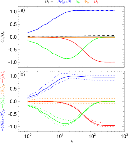
Figure 4: Spectral transfer in run 1. (a) The validity test $O_{k}$ of Eq. (24) (black solid line) as a function of $k$ along with the different contributions (solid lines): (blue) the losses/decay term $-\partial E_{\mathrm{k}k}/{\partial t}$, (green) the transfer term $-S_{k}$, (orange) the pressure dilatation term $\Psi_{k}$, and (red) the dissipation term $-D_{k}$. Dashed lines show the incompressible equivalent $O_{k}^{(i)}$ (Eq. (25)) and its contributions. (b) Time-averaged contributing terms (solid lines) with their minimum and maximum values (dotted lines) for (blue) the decay $-\langle\partial E_{\mathrm{k}k}/{\partial t}\rangle_{t}$, (green) the transfer $-\langle S_{k}\rangle_{t}$, (orange) the pressure dilatation term $\langle\Psi_{k}\rangle_{t}$, and (red) the dissipation term $-\langle D_{k}\rangle_{t}$. All the quantities are normalized with respect to $Q_{\mu}$.

Results from the ST approach in run 2 are shown in Fig. 5 in the same format as in Fig. 4. Fig. 5a is obtained for the times $t_{\omega}$ and $t_{\omega}+\Delta t$ as above. Eq. (18) is well satisfied in run 2, $|O_{k}|/Q_{\mu}<0.005$. Fig. 5a shows that the region dominated by dissipation is wider compared to run 2, owing to the larger viscosity. The energy containing region as well as the region where the energy transfer dominates are shifted to larger scales. Fig. 5a demonstrates the cumulative behavior of the low-pass filter in the $k$ space, Eq. (22). The pressure-dilatation term is stronger compared to that in run 1 and reaches the largest value on large $k$ (small scales). The error of the incompressible approach $O_{k}^{(i)}$ is larger and is not only connected with the pressure dilatation; the incompressible terms (especially the cascade one) noticeably differ from the compressible ones.

Fig. 5b shows that over the pressure-dilatation period the different components, $-\partial E_{\mathrm{k}k}/{\partial t}$, $-S_{k}$, $\Psi_{k}$, and $-D_{k}$ have very large temporal variations (large differences between the minimum and maximum values given by the dotted lines in Fig. 5b). The averaged pressure dilatation term is weak and exhibits small negative values over medium scales, a behavior qualitatively similar to that of the transfer $-S_{k}$. This indicates that the averaged effect of the pressure dilatation is a spectral transfer of the kinetic energy to smaller scales without a net exchange between kinetic and internal energies.

The observed spectra in Fig. 3 can be now interpreted using Figs. 4 and 5. The regions, where the compensated power spectra $Pk^{5/3}$ are about flat, correspond to regions where the energy transfer rate $S_{k}$ dominates. Large scales are dominated by the decay of $E_{\mathrm{k}k}$ and smaller scales are dominated by the dissipation.

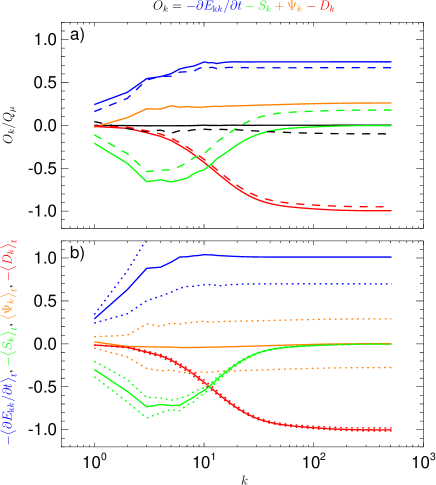
Figure 5: Spectral transfer in run 2 in the same format as in Fig. 4.

IV Kármán-Howarth-Monin equation

IV.1 Incompressible HD

In the incompressible HD (see Eq. (7)) the structure function

$$\mathcal{S}^{(i)}(\bm{l})=\langle|\delta\bm{u}|^{2}\rangle,$$ (26)

(where $\delta\bm{u}=\bm{u}(\bm{x}^{\prime})-\bm{u}(\bm{x})$, $\bm{x}^{\prime}=\bm{x}+\bm{l}$, and $\langle\bullet\rangle$ denotes spatial averaging) describes the kinetic-energy (per mass) spatial scale distribution and is related to the kinetic-energy power spectrum [1]. For statistically homogeneous decaying turbulence one can get the following dynamic KHM equation for the $\mathcal{S}^{(i)}$ [6, 7]

$$\frac{\partial\mathcal{S}^{(i)}}{\partial t}+\bm{\nabla}_{\bm{l}}\cdot\bm{\mathcal{Y}}^{(i)}=2\nu\Delta_{\bm{l}}\mathcal{S}^{(i)}-4\epsilon,$$ (27)

where

$$\bm{\mathcal{Y}}^{(i)}(\bm{l})=\left\langle\delta\bm{u}|\delta\bm{u}|^{2}\right\rangle;$$ (28)

$\epsilon$ is the incompressible heating rate (see Eq. 8). Eq. (27) is simply related to its original form that involves the cross-correlation $R(\bm{l})=\left\langle\bm{u}(\bm{x}^{\prime})\cdot\bm{u}(\bm{x})\right\rangle$ [1]

$$2\frac{\partial R(\bm{l})}{\partial t}-\bm{\nabla}_{\bm{l}}\cdot\bm{\mathcal{Y}}^{(i)}=4\nu\Delta_{\bm{l}}R(\bm{l})$$ (29)

since $S^{(i)}=2\langle|\bm{u}|^{2}\rangle-2R(\bm{l})$ and $\partial\langle|\bm{u}|^{2}\rangle/\partial t=-2\epsilon$. Eq. (27) relates the change of the second order structure function $\mathcal{S}^{(i)}$, $\partial\mathcal{S}^{(i)}/{\partial t}$, the dissipation rate $\epsilon$, the cross-scale transfer/cascade rate $\mathcal{K}^{(i)}=-\bm{\nabla}_{\bm{l}}\cdot\bm{\mathcal{Y}}^{(i)}/4$, and the dissipation term $\nu\Delta_{\bm{l}}\mathcal{S}^{(i)}$ (henceforth we drop the $\bm{l}$ subscript for $\bm{\nabla}$ and $\Delta$). The inertial range can be formally defined as the region where the decay and dissipation terms are negligible so that

$$\mathcal{K}^{(i)}=\epsilon.$$ (30)

For isotropic media, in the infinite Reynolds number limit, Eq. (30) leads to the so called exact (scaling) laws [8, 1]. Eq. (27) is more general and may be directly tested in numerical simulations [30], since large Reynolds numbers needed for existence of the inertial range are computationally challenging [31].

IV.2 Compressible HD

For the compressible Navier-Stokes equations, Eqs. (1,2), one possibility to describe the scale-distribution of kinetic energy is the structure function $\mathcal{S}=\left\langle\delta\bm{u}\cdot\delta\left(\rho\bm{u}\right)\right\rangle$ [21]. For the statistically homogeneous system one gets

$$\frac{\partial\mathcal{S}}{\partial t}+\bm{\nabla}\cdot\bm{\mathcal{Y}}+\mathcal{R}=4\varPsi-4\mathcal{D}+C_{\Psi}-C_{D},$$ (31)

where $\bm{\mathcal{Y}}=\left\langle\delta\bm{u}\left[\delta\left(\rho\bm{u}\right)\cdot\delta\bm{u}\right]\right\rangle$, $\mathcal{R}=\left\langle\delta\bm{u}\cdot\left(\theta^{\prime}\rho\bm{u}-\theta\rho^{\prime}\bm{u}^{\prime}\right)\right\rangle$, $\varPsi=\left\langle\delta p\delta\theta\right\rangle/2$, and $\mathcal{D}=\left\langle\delta\bm{\tau}:\delta\bm{\Sigma}\right\rangle/2$.

Here $C_{\varPsi}$ and $C_{\mathcal{D}}$ are correction terms to $\varPsi$ and $\mathcal{D}$ (that we choose to represent the pressure dilatation and the dissipation), respectively,

$$C_{\varPsi}=\mathcal{C}_{\rho}\left[\bm{u},\bm{\nabla}p\right],\ \ \ C_{\mathcal{D}}=\mathcal{C}_{\rho}\left[\bm{u},\bm{\nabla}\cdot\bm{\tau}\right],$$ (32)

where

$$\mathcal{C}_{\rho}\left[\bm{a},\bm{b}\right] =\left(\frac{\rho^{\prime}}{\rho}-1\right)\bm{a}^{\prime}\cdot\bm{b}+\left(\frac{\rho}{\rho^{\prime}}-1\right)\bm{a}\cdot\bm{b}^{\prime}.$$

Note that, the $C_{\varPsi}$ and $C_{\mathcal{D}}$ terms depend explicitly on the level of density fluctuations in the system.

$\mathcal{S}$ and $\bm{\mathcal{Y}}$ are compressible generalizations of $\mathcal{S}^{(i)}$ and $\bm{\mathcal{Y}}^{(i)}$, respectively. The $\mathcal{R}$ term presents an additional compressible energy-transfer channel [21] and likely corresponds to the compressible part in the spectral transfer, Eq. (19); we do not see an obvious way how to turn this term to a divergence form similar to $\bm{\nabla}\cdot\bm{\mathcal{Y}}$. The term $\varPsi$ is a structure-function formulation of the pressure dilatation effect $p\theta$. The viscous term $\mathcal{D}$ corresponds to a combination of the two dissipation terms in the incompressible case, $\epsilon-\nu\Delta\mathcal{S}^{(i)}/2$, in Eq. (27). On large scales, $|\delta\bm{x}|\rightarrow\infty$, the correlations $\left\langle{\bm{\tau}(\bm{x}^{\prime})}:\bm{\Sigma}\right\rangle\rightarrow 0$, and the viscous term becomes the viscous heating rate $Q_{\mu}$,

$$\mathcal{D}\rightarrow\left\langle\bm{\tau}:\bm{\Sigma}\right\rangle=Q_{\mu}.$$

The inertial range may be defined as the interval in the space of separation scales $\bm{l}$ where

$$\mathcal{K}=Q_{\mu}$$ (33)

where $\mathcal{K}=-(\bm{\nabla}\cdot\bm{\mathcal{Y}}+\mathcal{R})/4$ is the cascade/energy transfer term. Eq. (33) corresponds to the ST relation (Eq. (23)) and also neglects the pressure-dilatation effect. Now we can use Eq. (31) to interpret the simulation results. We define the departure from zero of this equation as

$$\mathcal{O}(l) =-\frac{1}{4}\frac{\partial\mathcal{S}}{\partial t}+\mathcal{K}+\varPsi^{\prime}-\mathcal{D}^{\prime}.$$ (34)

where the correction terms were included in $\varPsi^{\prime}$ and $\mathcal{D}^{\prime}$, $\varPsi^{\prime}=\varPsi+C_{\varPsi}/2$ and $\mathcal{D}^{\prime}=\mathcal{D}+C_{\mathcal{D}}/2$.

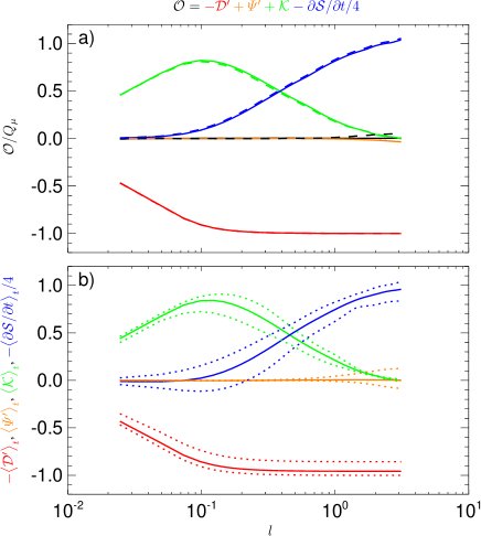
Figure 6: KHM equation for run 1: (a) The validity test $\mathcal{O}$ of Eq. (34) (black solid line) as a function of the separation scale $l$ along with the different contributions, (blue) $-{\partial\mathcal{S}}/{\partial t}/4$, (green) $\mathcal{K}$, (orange) $\Psi^{\prime}$, and (red) $-D^{\prime}$. Dashed lines show the incompressible equivalents. (b) Time-averaged contributing terms (solid lines) with their minimum and maximum values (dotted lines) for (blue) $-\langle{\partial\mathcal{S}}/{\partial t}\rangle_{t}/4$, (green) $\langle\mathcal{K}\rangle_{t}/4$, (orange) $\langle\varPsi^{\prime}\rangle_{t}$, and (red) $-\langle\mathcal{D}^{\prime}\rangle_{t}$. All the quantities are normalized with respect to $Q_{\mu}$.

The calculation of structure functions in 3D is computationally demanding thus the KHM analysis is done on a $256^{3}$ box (taking every fourth point in all directions). The structure functions are calculated over the 3D separation space and isotropized/averaged over the solid angle. The partial time derivative is approximated by the finite difference between the two times. Fig. 6a shows the validity test $\mathcal{O}$ in run 1 as a function of the scale $l=|\bm{l}|$ along with the different contributions, the decay term $-{\partial\mathcal{S}}/{\partial t}/4$, the energy transfer/cascade term $\mathcal{K}$, the pressure dilatation term $\varPsi^{\prime}$, and the dissipation term $-\mathcal{D}^{\prime}$. Eq. (31) is well satisfied in run 1, the departure from validity is small, $|\mathcal{O}|/Q_{\mu}<0.005$; this error is due to the finite difference estimation of $\partial\mathcal{S}/\partial t$ (as in the spectral transfer case).

On large scales, the compressible dissipation term $\mathcal{D}\rightarrow Q_{\mu}$ as expected. Similarly, $\partial\mathcal{S}/\partial t/4\rightarrow\partial E_{\mathrm{k}}/\partial t\sim-Q_{\mu}$. The pressure-dilatation term is small and appears only on large scales. The cascade term is important on medium scales but there is no true inertial range, since both the decay and the dissipation are not negligible there. Run 1 is weakly compressible, the compressible energy-transfer term $\mathcal{R}$ is small ($|\mathcal{R}|/Q_{\mu}<0.03$). Also the correction terms are negligible ($|C_{\varPsi}|/Q_{\mu}<0.006$ and $|C_{\mathcal{D}}|/Q_{\mu}<0.002$).

Fig. 6a displays by dashed lines results of the corresponding incompressible version of KHM equation, the validity test given by

$$\mathcal{O}^{(i)}(l)=-\frac{1}{4}\frac{\partial\mathcal{S}^{(i)}}{\partial t}+\mathcal{K}^{(i)}+\frac{1}{2}\nu\Delta\mathcal{S}^{(i)}-\epsilon.$$ (35)

The incompressible terms are comparable to their compressible counterparts, in particular, the dissipation terms are close to each other since the dissipation is mostly incompressible (see Fig. 1e). The incompressible error $\mathcal{O}^{(i)}$ appears on large scales and is related to the missing pressure-dilatation term, in agreement with the ST results.

Fig. 6b displays the results of the KHM equation averaged over one pressure-dilatation oscillation period. The colored solid lines show the time averaged quantities, the decay term $-\partial\mathcal{S}/\partial t/4$, the energy transfer/cascade term $\mathcal{K}$, the pressure dilatation term $\varPsi^{\prime}$, and the scale-dependent dissipation term $-\mathcal{D}^{\prime}$. The colored dotted lines shows the corresponding minimum and maximum values. The averaged pressure-dilatation effect is negligible even though the variation is of the order $0.1Q_{\mu}$. Similar variations are seen also in other terms.

The results for the more compressible run 2 are shown in Fig. 7. Fig. 7a displays by solid lines the results for the time $t_{\omega}$ and $t_{\omega}+\Delta t$, the error check $\mathcal{O}$ as a function of $l$ along with the different contributions. Eq. (31) is also well satisfied in run 2, the departure from validity is small, $|\mathcal{O}|/Q_{\mu}<0.01$. The KHM approach exhibits cumulative properties similar to those of the ST approach (Eq. (22)). The compressible dissipation term $\mathcal{D}\rightarrow Q_{\mu}$ on large scales as expected, Similarly, $\partial\mathcal{S}/\partial t/4\rightarrow\partial E_{\mathrm{k}}/\partial t\simeq-0.7Q_{\mu}$ and $\varPsi^{\prime}\rightarrow\langle p\theta\rangle\simeq 0.3Q_{\mu}$. On large scales we recover the energy conservation $\partial E_{\mathrm{k}}/\partial t=\langle p\theta\rangle-Q_{\mu}$.

Dashed lines on Fig. 7a show the incompressible results, $\mathcal{O}^{(i)}$ and its constituents. The incompressible KHM equation is not applicable in run 2: the error $\mathcal{O}^{(i)}$ is substantial and is not simply related to the pressure dilatation, an important part of dissipation is compressible (see Fig. 2e), and the incompressible transfer rate, $\mathcal{K}^{(i)}$, departs strongly from the compressible one $\mathcal{K}$. This is partly due to the compressible energy-transfer term $\mathcal{R}$ that becomes important ($|\mathcal{R}|/Q_{\mu}<0.7$). In run 2, the correction terms are not negligible ($|C_{\varPsi}|/Q_{\mu}<0.3$ and $|C_{\mathcal{D}}|/Q_{\mu}<0.1$).

It is interesting that for run 2 the incompressible approximation overestimates the energy-transfer rate in the KHM approach whereas for the ST method the incompressible equation gives an energy-transfer rate that is lower than the compressible one (see Fig. 5a). The incompressible approximation is not generally valid, however, it may possibly be useful to locate the inertial range.

The different contributing terms of Eq. (31) time-averaged over one pressure-dilatation oscillation are shown in Fig. 7b. All the quantities (except the dissipation one) exhibit large variations, mainly on large scales. The averaged pressure-dilatation term, $\langle\varPsi^{\prime}\rangle_{t}$, is about zero on large and small scales and reaches the maximum $\simeq 0.05Q_{\mu}$ at about $l=20$. The positive value of $\langle\varPsi^{\prime}\rangle_{t}$ suggests that the pressure-dilatation effect leads to a transfer of the kinetic energy from large to smaller scales, while there is no net energy exchange between the kinetic and internal energies, in agreement with the ST results.

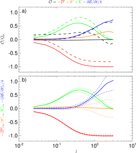
Figure 7: KHM equation for run 2 in the same format as in Fig. 6.

Note that the choice $\delta(\rho\bm{u})\cdot\delta\bm{u}$ corresponds in the ST approach to $\Re\widehat{\rho\bm{u}}\cdot\widehat{\bm{u}}^{*}$ [32]. For the ST equation with $|\widehat{\bm{w}}|^{2}$ [17, 12] (see Eq. (18)) one can obtain an alternative KHM equation taking $\mathcal{S}_{w}=\left\langle|\delta\bm{w}|^{2}\right\rangle$ as

$$\frac{\partial\mathcal{S}_{w}}{\partial t}+\bm{\nabla}_{\bm{l}}\cdot\bm{\mathcal{Y}}_{w}+\mathcal{R}_{w}=4\varPsi-4\mathcal{D}+C_{\varPsi w}-C_{\mathcal{D}w},$$ (36)

where

$$\bm{\mathcal{Y}}_{w}=\left\langle\delta\bm{u}|\delta\bm{w}|^{2}\right\rangle,\ \ \ \mathcal{R}_{w}=\left\langle\delta\bm{w}\cdot\left(\theta^{\prime}\bm{w}-\theta\bm{w}^{\prime}\right)\right\rangle$$ (37)

$$C_{\varPsi w}=2\mathcal{C}_{\sqrt{\rho}}\left[\bm{u},\bm{\nabla}p\right],\ \ \ C_{\mathcal{D}w}=2\mathcal{C}_{\sqrt{\rho}}\left[\bm{u},\bm{\nabla}\cdot\bm{\tau}\right],$$ (38)

For the two weakly compressible runs presented here these two variants of the KHM relation give almost identical results.

IV.3 Comparison

For both the runs, the ST and KHM equations give quantitatively analogous results. This is not surprising, $E_{\mathrm{k}k}$ represents a low-pass filtered spectral distribution of the kinetic energy whereas $\mathcal{S}$ represents the kinetic energy at the separation scales smaller than $l$ (corresponding to a high-pass filter), and similar differences apply to the other terms. A remaining question is the relationship between the wave vector $k$ and the scale separation $l$. Since the two quantities should be inversely proportional, we tested different factors $\alpha$ in $k=\alpha/l$. For $\alpha=\sqrt{3}$ the ST and KHM results get close to each other.

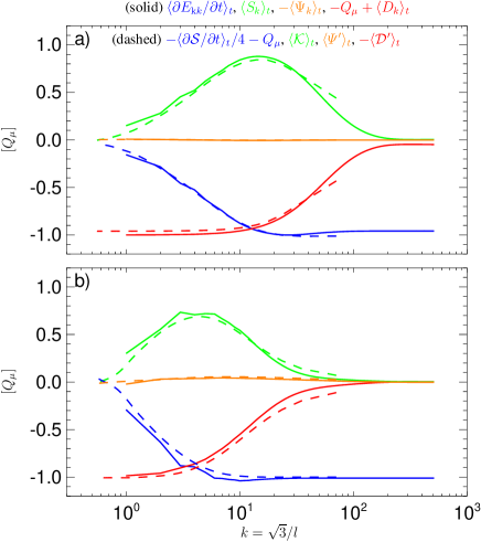
Figure 8: Direct comparison between ST and KHM methods for (a) run 1 and (b) run 2: Solid lines denote the time-averaged ST terms (see Figs. 4 and 5): (blue) the losses/decay $\langle\partial E_{\mathrm{k}k}/{\partial t}\rangle_{t}$, (green) the transfer $\langle S_{k}\rangle_{t}$, (orange) the pressure dilatation term $-\langle\Psi_{k}\rangle_{t}$, and (red) the dissipation term $\langle D_{k}\rangle_{t}-Q_{\mu}$ (i.e., shifted by $Q_{\mu}$) as functions of $k$. Dashed lines denote the corresponding time-averaged KHM contributions (see Figs. 6 and 7): (blue) $-\langle{\partial\mathcal{S}}/{\partial t}\rangle_{t}/4-Q_{\mu}$ (i.e., shifted by $Q_{\mu}$), (green) $\mathcal{K}$, (orange) $\langle\Psi^{\prime}\rangle_{t}$, and (red) $-\langle\mathcal{D}^{\prime}\rangle_{t}$ as functions of $l=\sqrt{3}/k$. All the quantities are normalized with respect to $Q_{\mu}$.

Fig. 8 shows that in both runs, for $k=\sqrt{3}/l$, the time-averaged cascade rates obtained from the ST and KHM relations are comparable $\langle S_{k}\rangle_{t}\simeq\langle\mathcal{K}\rangle_{t}$; the same is true for the pressure-dilatation induced cross-scale transfers $\langle\Psi_{k}\rangle_{t}\simeq-\langle\varPsi\rangle_{t}$.

The decay and dissipation terms have comparable behaviors when shifted by the dissipation rate $Q_{\mu}$. This may be expressed as (here we leave out the time averages)

$$\frac{\partial E_{\mathrm{k}k}}{\partial t}+\frac{1}{4}\frac{\partial\mathcal{S}}{\partial t} \simeq-Q_{\mu},\ \ \ D_{k}+\mathcal{D}^{\prime}\simeq Q_{\mu},$$ (39)

the ST and KHM quantities are complementary as expected. As $\partial E_{\mathrm{k}k}/{\partial t}$ represents the rate of change of the kinetic energy on scales with wave-vector magnitudes smaller or equal to $k$, ${\partial\mathcal{S}}/{\partial t}/4$ gives approximatively the remaining decay rate (for wave-vector magnitudes larger than $k$). Similarly, $D_{k}$ is the dissipation rate on the scales $\leq k$ whereas $\mathcal{D}^{\prime}$ represents about the complementary dissipation rate (on the scales $>k$).

V Internal Energy

In the previous section, we showed that the exchanges between the kinetic and internal energies lead to a transfer of kinetic energy from large to small scales. It is, therefore, interesting to look at the scale dependence of the internal energy and its cross-scale transfer.

V.1 Spectral transfer

One possible description of the spectral scale decomposition and cross-scale transfer of the internal energy could be done through the variable $q=(\gamma\rho T)^{1/2}$ [17]. Its evolution, following from Eq. (3), is given by

$$\frac{\partial q}{\partial t}+\left(\bm{u}\cdot\bm{\nabla}\right)q+\frac{1}{2}q\theta= \frac{\alpha\gamma}{2}\frac{1}{q}\Delta T-\frac{1}{2}\gamma\left(\gamma-1\right)\frac{1}{q}p\theta$$ (40)

$$+\frac{1}{2}\gamma\left(\gamma-1\right)\frac{1}{q}\bm{\Sigma}:\bm{\tau}.$$

We set the spectral decomposition of the internal energy, analogously to the case of the kinetic one, as low-pass filtered quantity

$$E_{\mathrm{i}k}=\frac{1}{\gamma\left(\gamma-1\right)}\sum_{|\bm{k}^{\prime}|\leq k}|\widehat{q}|^{2}.$$ (41)

For $E_{\mathrm{i}k}$, one gets the following dynamic equation

$$\frac{\partial E_{\mathrm{i}k}}{\partial t}+S_{\mathrm{i}k}=\Phi_{\mathrm{i}k}-\Psi_{\mathrm{i}k}+D_{\mathrm{i}k}$$ (42)

where

$$S_{\mathrm{i}k} =\frac{1}{\gamma\left(\gamma-1\right)}\Re\sum_{|\bm{k}^{\prime}|\leq k}\left[2\widehat{q}^{*}\widehat{\left(\bm{u}\cdot\bm{\nabla}\right)q}+\widehat{q}^{*}\widehat{q\theta}\right],$$

$$\Psi_{\mathrm{i}k} =\frac{1}{\gamma}\Re\sum_{|\bm{k}^{\prime}|\leq k}\widehat{q}^{*}\widehat{q\theta},\ \ \ D_{\mathrm{i}k}=\Re\sum_{|\bm{k}^{\prime}|\leq k}\widehat{q}^{*}\widehat{q^{-1}\bm{\Sigma}:\bm{\tau}},$$

$$\Phi_{\mathrm{i}k} =\frac{\alpha}{\left(\gamma-1\right)}\Re\sum_{|\bm{k}^{\prime}|\leq k}\widehat{q}^{*}\widehat{q^{-1}\Delta T}.$$ (43)

Here $S_{\mathrm{i}k}$ describes the cross-scale energy transfer, $\Phi_{\mathrm{i}k}$ results from the thermal diffusion, $\Psi_{\mathrm{i}k}$ is a term representing the pressure-dilatation effect, and $D_{\mathrm{i}k}$ comes from the viscous heating.

As there is no clear pressure-dilation induced cross-scale transfer in run 1, we look only at run 2. We define the validity test of Eq. (42) as before by

$$O_{\mathrm{i}k}=-\frac{\partial E_{\mathrm{i}k}}{\partial t}-S_{\mathrm{i}k}+\Phi_{\mathrm{i}k}-\Psi_{\mathrm{i}k}+D_{\mathrm{i}k}.$$ (44)

Fig. 9a displays $O_{\mathrm{i}k}$, and its constituents, obtained at $t_{\omega}$ and $t_{\omega}+\Delta t$. Eq. (42) is well satisfied, $|O_{\mathrm{i}k}|/Q_{\mu}<0.007$. $\partial E_{\mathrm{i}k}/{\partial t}$ is positive as the internal energy increases and varies mostly on large scales. $D_{\mathrm{i}k}$ is about constant $\sim Q_{\mu}$. This is due the fact that the nonlinear term $\bm{\tau}:\bm{\Sigma}$ heats everywhere in the simulation box and importantly contributes to the $k=0$ term. The pressure-dilatation term varies on large scales, the diffusion and the transfer term lead to weak scale redistribution of the internal energy.

Fig. 9b shows the spectral transfer results averaged over one pressure-dilatation oscillation period, the mean values of the different terms and their minimum and maximum values. The dissipation, $\langle D_{\mathrm{i}k}\rangle_{t}\simeq Q_{\mu}$ with weak variations, $\langle\partial E_{\mathrm{i}k}/{\partial t}\rangle_{t}\simeq Q_{\mu}$ with large temporal variations. The pressure dilatation $\langle\Psi_{\mathrm{i}k}\rangle_{t}$ is small and negative (with large fluctuations). The diffusion $\langle\Psi_{\mathrm{i}k}\rangle_{t}$ is weak with positive values and the cross-scale transfer $\langle S_{\mathrm{i}k}\rangle_{t}$ is small with large fluctuations of large scales. In analogy with the spectral analysis for the kinetic energy, the nonlinear term $S_{\mathrm{i}k}$ leads to transfer of the internal energy from large to small scales whereas the diffusion and the pressure dilatation lead to transfer of the internal energy in the opposite direction. These processes roughly compensate each other and the dominant energy channel is the viscous heating $\langle\partial E_{\mathrm{i}k}/{\partial t}\rangle_{t}\simeq\langle D_{\mathrm{i}k}\rangle_{t}$. It is also clear that the dynamic spectral description of the internal energy, Eq. (42), is hardly comparable to that for the kinetic energy, Eq. (18), especially concerning the viscous dissipation, compare Figs. 5 and 9. On the other hand, the pressure-dilatation terms for the kinetic (Eq. (18)) and internal (Eq. (42)) energies are comparable, $\Psi_{\mathrm{i}k}\simeq\Psi_{k}$. For the combined quantity $E_{\mathrm{k}k}+E_{\mathrm{i}k}$ the pressure-dilatation terms cancel each other as one may expect. On the other hand, the dissipation terms have very different scale representations, so that $E_{\mathrm{k}k}+E_{\mathrm{i}k}$ clearly does not represent the total energy, the kinetic and internal energies ought to be treated separately.

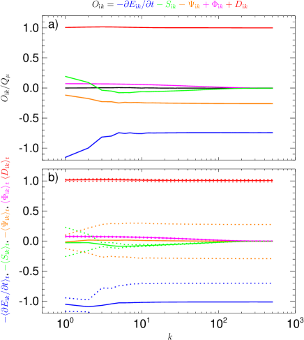
Figure 9: Spectral transfer of the internal energy in run 2: (a) The validity test $O_{\mathrm{i}k}$ of Eq. (44) (black line) as a function of $k$ along with the different contributions, (blue) the time variation $-\partial E_{\mathrm{i}k}/{\partial t}$, (green) the energy transfer term $-S_{\mathrm{i}k}$, (orange) the pressure dilatation term $\Psi_{\mathrm{i}k}$, (magenta) the diffusion $\Phi_{\mathrm{i}k}$, and (red) the dissipation term $D_{\mathrm{i}k}$. (b) Time-averaged contributing terms (solid lines) with their minimum and maximum values (dotted lines) for (blue) the decay $-\langle\partial E_{\mathrm{i}k}/{\partial t}\rangle_{t}$, (green) the transfer $-\langle S_{\mathrm{i}k}\rangle_{t}$, (orange) the pressure dilatation term $\langle\Psi_{\mathrm{i}k}\rangle_{t}$, (magenta) the diffusion $\langle\Phi_{\mathrm{i}k}\rangle_{t}$, and (red) the dissipation term $\langle D_{\mathrm{i}k}\rangle_{t}$. All the quantities are normalized with respect to $Q_{\mu}$.

V.2 KHM equation

One way to represent the internal energy in the KHM approach is the structure function [21]

$$\mathcal{S}_{\mathrm{i}}=\left\langle\delta\rho\delta e\right\rangle.$$ (45)

From Eq. (3), it follows for $e$

$$\rho\frac{\partial e}{\partial t}+\rho(\bm{u}\cdot\bm{\nabla})e=\alpha\Delta e-p\theta+\bm{\tau}:\bm{\Sigma}$$ (46)

and for $\mathcal{S}_{\mathrm{i}}$ one gets the dynamic KHM-like equation

$$\frac{\partial\mathcal{S}_{\mathrm{i}}}{\partial t}+\bm{\nabla}\cdot\bm{\mathcal{Y}}_{\mathrm{i}}+\mathcal{R}_{\mathrm{i}} =2\varPhi_{\mathrm{i}}-2\varPsi_{\mathrm{i}}+2\mathcal{D}_{\mathrm{i}}$$ (47)

where

$$\bm{\mathcal{Y}}_{\mathrm{i}} =\left\langle\delta\bm{u}\delta\rho\delta e\right\rangle,\ \ \ \mathcal{R}_{\mathrm{i}}=\left\langle(\rho\theta^{\prime}-\rho^{\prime}\theta)\delta e\right\rangle,$$

$$\varPsi_{\mathrm{i}} =\mathcal{V}_{\rho}\left(p\theta\right)/2,\ \ \ \mathcal{D}_{\mathrm{i}}=\mathcal{V}_{\rho}\left(\bm{\tau}:\bm{\Sigma}\right)/2$$

$$\varPhi_{\mathrm{i}} =\alpha\left\langle\delta\rho\delta\left(\rho^{-1}\Delta e\right)\right\rangle/2,$$ (48)

and

$$\mathcal{V}_{\rho}\left(a\right) =\left\langle\left(1-\frac{\rho}{\rho^{\prime}}\right)a^{\prime}+\left(1-\frac{\rho^{\prime}}{\rho}\right)a\right\rangle$$

In Eq. (47) $\mathcal{K}_{\mathrm{i}}=-(\bm{\nabla}\cdot\bm{\mathcal{Y}}_{\mathrm{i}}+\mathcal{R}_{\mathrm{i}})/2$ represents the cross-scale transfer connected with $\mathcal{S}_{\mathrm{i}}$.

The pressure-dilatation $\varPsi_{\mathrm{i}}$ and the dissipation $\mathcal{D}_{\mathrm{i}}$ terms depend on the density variation; for a constant $\rho$ these terms disappear. This is the first indication that $\mathcal{S}_{\mathrm{i}}$ does not represent the internal energy in a way comparable to the kinetic energy structure function $\mathcal{S}$.

To test Eq. (47) on the simulation results of run 2 we define the departure as

$$\mathcal{O}_{\mathrm{i}}(l) =-\frac{1}{2}\frac{\partial\mathcal{S}_{\mathrm{i}}}{\partial t}+\mathcal{K}_{\mathrm{i}}+\Phi_{\mathrm{i}}-\Psi_{\mathrm{i}}+D_{\mathrm{i}}.$$ (49)

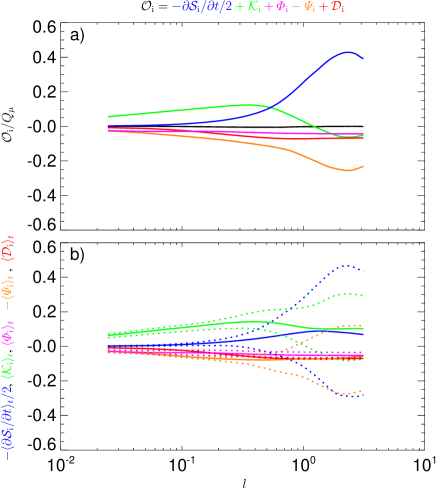
Figure 10: KHM equation for the internal energy in run 2: (a) The validity test $\mathcal{O}_{\mathrm{i}}$ of Eq. (49) (black line) as a function of the separation scale $l$ along with the different contributions, (blue) $-{\partial\mathcal{S}_{\mathrm{i}}}/{\partial t}/2$, (green) $\mathcal{K}_{\mathrm{i}}$, (orange) $-\varPsi_{\mathrm{i}}$, (red) $\mathcal{D}_{\mathrm{i}}$, and (magenta) $\varPhi_{\mathrm{i}}$. (b) Time-averaged contributing terms (solid lines) with their minimum and maximum values (dotted lines) for (blue) $-\langle{\partial\mathcal{S}_{\mathrm{i}}}/{\partial t}\rangle_{t}/2$, (green) $\langle\mathcal{K}_{\mathrm{i}}\rangle_{t}$, (orange) $-\langle\varPsi_{\mathrm{i}}\rangle_{t}$, (red) $\langle\mathcal{D}_{\mathrm{i}}\rangle_{t}$, and (magenta) $\langle\varPhi_{\mathrm{i}}\rangle_{t}$. All the quantities are normalized with respect to to $Q_{\mu}$.

Fig. 10a shows the departure (black) $\mathcal{O}_{\mathrm{i}}$ as a function of the scale $l$ along with the different contributions, the decay term (blue) $-{\partial\mathcal{S}_{\mathrm{i}}}/{\partial t}/2$, the energy transfer term (green) $\mathcal{K}_{\mathrm{i}}$, the pressure dilatation term (orange) $-\varPsi_{\mathrm{i}}$, (red) the dissipation term $\mathcal{D}_{\mathrm{i}}$, and the diffusion term (magenta) $\varPhi_{\mathrm{i}}$. The calculation is done on a sub-grid of $256^{3}$. Eq. (47) is well satisfied, $|\mathcal{S}_{\mathrm{i}}|/Q_{\mu}<0.005$.

The pressure dilatation structure function terms for the kinetic (Eq. (31)) and internal (Eq. (47)) energies are similar, $\varPhi_{\mathrm{i}}\simeq\varPhi$. The diffusion term is small and (except for the sign) corresponds the diffusion term in the ST approach (Eq. (42)). The dissipation terms is small with respect to the dissipation rate $Q_{\mu}$, indicating that the viscous heating is not well represented in Eq. (47). Consequently, the structure function $\mathcal{S}_{\mathrm{i}}=\left\langle\delta\rho\delta e\right\rangle$ decreases with time in contrast with the internal energy $E_{\mathrm{i}}=\langle\rho e\rangle$ that increases (see Fig. 2). These properties remain unchanged even after averaging over one pressure-dilatation oscillation period as displayed in Fig. 10b. All the terms (except the dissipation and diffusion ones) exhibit large variations, dominantly on the large scales. The averaged pressure-dilatation term is small and corresponds to that of the kinetic energy, $\langle\varPhi_{\mathrm{i}}\rangle_{t}\simeq\langle\varPhi\rangle_{t}$.

Combining Eq. (31) with Eq. (47) as $\partial(\mathcal{S}/2+\mathcal{S}_{\mathrm{i}})/\partial t$ one recovers to a large extent the results of Ref. 21 (note, however, that the pressure-dilatation effects are in Ref. 21 transformed to a contribution to the cascade term using the isothermal closure). For the combined quantity $\mathcal{S}/2+\mathcal{S}_{\mathrm{i}}$ the pressure-dilation terms cancel each other, similar to the ST case. However, the scale-dependence of the viscous dissipation/heating is significantly different in the two approaches, so that it is hard to interpret $\mathcal{S}/2+\mathcal{S}_{\mathrm{i}}$ as a representative of the total energy. The kinetic and internal energies are better to be investigated separately by Eq. (31) and Eq. (47).

The choice $\delta\rho\delta e$ does not correspond to the ST equation in the previous section based on $|\widehat{q}|^{2}$ [17]. In order to get an alternative version of the internal energy KHM equation corresponding to Eq. (42), one can investigate $|\delta q|^{2}$. The resulting equation can be expressed in a form similar to Eq. (47) as

$$\frac{\partial\mathcal{S}_{\mathrm{i}q}}{\partial t}+\bm{\nabla}\cdot\bm{\mathcal{Y}}_{\mathrm{i}q}+\mathcal{R}_{\mathrm{i}q} =\varPhi_{\mathrm{i}q}-\varPsi_{\mathrm{i}q}+\mathcal{D}_{\mathrm{i}q}$$ (50)

where

$$\mathcal{S}_{\mathrm{i}q} =\frac{1}{\gamma\left(\gamma-1\right)}\left\langle|\delta q|^{2}\right\rangle,\ \ \ \bm{\mathcal{Y}}_{\mathrm{i}q}=\frac{1}{\gamma\left(\gamma-1\right)}\left\langle\delta\bm{u}|\delta q|^{2}\right\rangle,$$

$$\mathcal{R}_{\mathrm{i}q} =\frac{1}{\gamma\left(\gamma-1\right)}\left\langle\delta q(q\theta^{\prime}-q^{\prime}\theta)\right\rangle,$$

$$\varPsi_{\mathrm{i}q} =\left\langle\delta q\delta\left(q^{-1}p\theta\right)\right\rangle,\ \ \ \mathcal{D}_{\mathrm{i}}=\left\langle\delta q\delta\left(q^{-1}\bm{\Sigma}:\bm{\tau}\right)\right\rangle,$$

$$\varPhi_{\mathrm{i}q} =\frac{\alpha}{\left(\gamma-1\right)}\left\langle\delta q\delta\left(q^{-1}\Delta T\right)\right\rangle.$$ (51)

Analysing run 2 using this form of the internal energy KHM equation we obtain results similar to those in Fig. 10. Therefore, also Eq. (50) is to be investigated separately from Eq. (47).

VI Discussion

In this paper we investigated the properties of the spectral/spatial-scale distribution and the cross-scale transfer of the kinetic energy in compressible hydrodynamic turbulence. We used the dynamic spectral transfer (ST) Kármán-Howarth-Monin (KHM) equations, in compressible and incompressible forms, to analyze results of two 3D direct numerical simulations of decaying compressible turbulence simulation with moderate Reynolds numbers and the initial Mach numbers $M=1/3$ and $M=1$. The simulations are initiated with large-scale solenoidal velocity fluctuations. The nonlinear coupling leads to a flux of the kinetic energy to small scales where it is dissipated; at the same time, the reversible pressure-dilatation mechanism causes oscillatory exchanges between the kinetic and internal energies with an average zero net energy transfer. While the simulations do not exhibit a clear inertial range, owing largely to moderate Reynolds numbers, the dynamic compressible KHM and ST equations are well satisfied in the simulations. These approaches describe, in a quantitatively similar way for both the methods, the decay of the kinetic energy on large scales, the energy transfer/cascade, the pressure dilatation, and the dissipation process. The incompressible versions are not valid, especially in run 2 (starting with $M=1$).

The ST approach that uses a low-pass filter in the $k$ space is by construction cumulative; in particular, the dissipation ST term reaches its (absolute) maximum values (given by the dissipation rate) at large $k$ (small scales). The KHM approach is complementary and has similar cumulative properties but in the opposite direction: the dissipation KHM term reach its (absolute) maximum values at large scales (given as well by the dissipation rate). The comparison between the two approaches demonstrates that the range of scales where the dissipation is important is determined by the variations/gradients of the ST and KHM dissipation terms rather than their values. The same applies to the pressure dilatation: the pressure-dilatation terms in the ST and KHM exhibit opposite cumulative properties, they approaches reach the average pressure dilatation at small and large scales, respectively. These results indicate that analyses based on the values of the cumulative pressure-dilatation terms are not very relevant; it is the variation over scales that counts. The pressure-dilatation energy exchange between the kinetic and internal energy gets negligible when averaged over a period of pressure-dilatation oscillations. The time-averaged pressure dilatation may lead to a transfer of the kinetic energy from large to small scales (in agreement with Ref. 20). For much larger systems we expect that the pressure-dilatation energy exchange becomes negligible for any given time. This may explain the apparent discrepancy between the results of Refs. 19, 12 and Ref. 20.

The results of both the simulations indicate a simple relationship between the KHM and ST results through the inverse proportionality between the wave vector $k$ and the spatial separation length $l$ as $kl\simeq\sqrt{3}$ and suggest a complementary scale-distribution meaning of the ST and KHM quantities. Interestingly, preliminary results of a similar comparison in two-dimensional Hall MHD simulations suggest a similar dependence $kl\simeq\sqrt{2}$ indicating that the relationship between the two scales depends on the space dimension. The simple relationship is useful to interpret the KMH results in the context of spectral analyses.

The ST approach is straightforward, requires less computational resources, and is directly linked to the spectral properties of velocity fluctuations. The KHM is more computationally demanding but leads to the so called exact scaling laws, and can be directly used to analyze anisotropic turbulence [33, 23]. We obtained similar results from the coarse-graining approach [34]. The coarse-graining approach presents semi-quantitatively similar results concerning the energy-transfer/cascade, decay, dissipation, and the pressure dilatation processes; the localization of these different processes is, however, somewhat different when expressed in space-filtering scales with respect to the spatial separation scale. The cumulative features of the coarse-graining approach is similar to that of the KHM equation by construction (spatial low-pass filter) but more detailed comparison between the coarse-graining method and the ST and KHM ones is beyond the scope of this paper.

We also investigated the properties of the internal energy using dynamic ST and KHM equations. These equations are well satisfied in both the simulations and the descriptions of the pressure-dilation effect are compatible with their counterpart for the kinetic energy. The ST and KHM equations for the kinetic and internal energies behave, however, very differently with respect to the viscous dissipation. Consequently, the ST and KHM (and likely also coarse-graining) approaches should better be used for the kinetic and internal energies separately. Moreover, the pressure-dilatation reversible coupling does not appear to lead to a net energy transfer between the kinetic and internal energies, at least in weakly compressible systems. It is, therefore, not necessary to investigate the two energies combined. The usage of combined quantities [21, 22] may lead to questionable results. For instance, in order to determine heating rates of the turbulent cascade it is necessary to look at the behavior of the kinetic energy (plus the magnetic energy in the magnetohydrodynamic case); the cascade/cross-scale transfer of the internal energy just leads to its redistribution.

Ref. 19 analyzed the pressure-dilatation effect and showed it decreases rapidly from large to small scales so that for a large enough system there are scales where the pressure dilatation becomes negligible and where the kinetic energy cascades in a conservative manner owing to the nonlinear advection term. Our results further suggest that on larger scales the kinetic energy is also conservatively transferred from large to small scales, partly owing to the standard nonlinear-advection cascade and partly to the pressure-dilatation-induced energy transfer (the locality of the latter process is unclear). Our simulation results are limited by moderate Reynolds numbers and weak compressibilities, so they need to be extended to larger Reynolds number and higher Mach numbers [31, 14, 35, 36, 37].