Gauge covariant neural network for quarks and gluons

Abstract

Quantum-Chromo dynamics (QCD) is a fundamental theory for quarks and gluons, which describes both the sub-atomic world and the history of our universe. The simulation for QCD on a lattice (lattice QCD) is one of the most challenging computational tasks. Recently, machine-learning techniques have been applied to solve various problems in lattice QCD. We propose gauge covariant neural networks and their training rule for lattice QCD, which can treat realistic quarks and gluons in four dimensions. We find that the smearing procedure can be regarded as extended versions of residual neural networks with fixed parameters. To show the applicability of our neural networks, we develop the self-learning hybrid Monte-Carlo for two-color QCD, where results are consistent with the results of the Hybrid Monte Carlo.

I Introduction

Convolutional neural networks (CNNs) have been one of the most successful methods in the field of machine learning, especially in image recognition (Fig. 1 (a) top) [1, 2]. One of the reasons is the network structure that makes the output identical from input data that can be shifted from one to the other by translational operations. Considering the network structure as a filter on the input data, the CNNs can be regarded as a trainable filter that respects the symmetry (Fig. 1 (a) bottom).

(a)

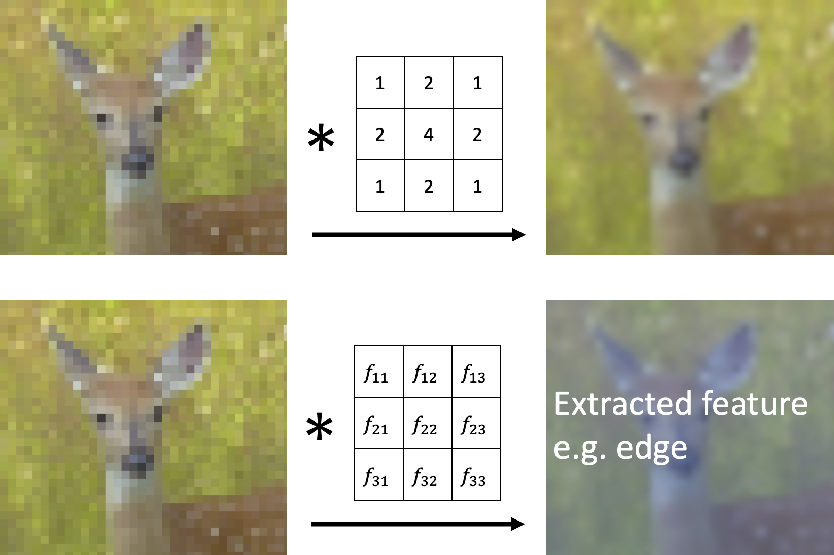
(b)

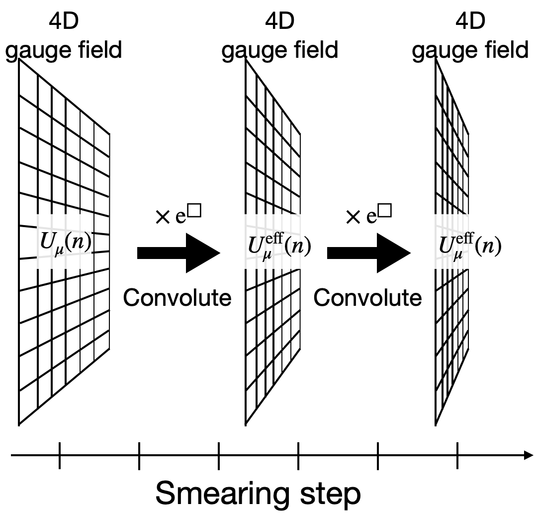
Figure 1: Schematic figures of filtering, CNN, and smearing. (Top of a) Images are smoothened by the Gaussian filter ($3\times 3$). (Bottom of a) Images are fed in the convolutional layer, which is a trainable filter, and the operation is determined by training. (b) Schematic figure of the stout smearing [3]. The gauge configuration is smoothened in a covariant manner.

Continuous symmetries are critical concepts in theoretical physics. The energy-momentum tensor, a crucial observable in physics, is defined through the Noether theorem for a global translational symmetry. Quarks and gluons, fundamental building blocks of our world, are described by a non-Abelian gauge symmetric quantum field theory called quantum chromo-dynamics (QCD). Gauge symmetry is essential to keep renormalizability. Lattice QCD is one of the most successful formulations for calculating QCD, keeping gauge symmetry under a cutoff, reproducing the hadron spectrum, and predicting phase transition temperature and other quantities [4, 5, 6].

The smearing [7, 8, 3, 9], a smoothing technique for gauge fields (Fig. 1 (b)), has been used for reducing cutoff effects due to the finite-lattice spacing in lattice QCD [10, 11, 12, 13, 14]. We point out that the smearing can be regarded as a filter that respects important symmetries in lattice QCD: global translational, rotational, and $\mathop{\rm SU}(N_{c})$ gauge symmetries, where $N_{c}=2,3,4\cdots$ is the number of colors.

We introduce a trainable filter that respects $\mathop{\rm SU}(N_{c})$ gauge, and global lattice translation and rotational symmetries by regarding the smearing as the filter that maps between rank-2 tensor-valued vector fields. This trainable filter can be used in systems with quarks and gluons in any dimension since the smearing has been tested and studied in past decades. While the input data in the conventional CNNs consist of a set of real-valued scalar data, the input data in the smearing filter consist of a collection of complex-valued $\mathop{\rm SU}(N_{c})$ matrix data. We call this filter gauge covariant neural networks. As we will show, covariant neural networks can be trained by the extended delta rule, whose scalar-valued version is well known in machine-learning community. We find that the derivation of the extended delta rule with rank-2 tensor-valued vector fields is similar to the well-known derivation of the Hybrid Monte Carlo (HMC) force of smeared fermions [3, 8]. In other words, with the extended delta rule, one can easily obtain derivatives of any quantities with respect to the bare gauge links like the smeared force.

There are several methods with machine-learning techniques used for various kinds of purposes in lattice QCD [15, 16, 17, 18, 19, 20, 21, 22, 23]. Most characteristic feature of our neural networks is that dynamical fermions can be treated naturally. In this paper, to demonstrate the potential application of our neural networks, we perform a simulation with self-learning hybrid Monte-Carlo (SLHMC) [24] for non-Abelian gauge theory with dynamical fermions. SLHMC uses a parametrized fermion action in the molecular dynamics, and we employ a gauge covariant neural network to parametrize the action for a fermion.

This paper is organized as follows. We introduce a neural network with covariant layers, which can process non-Abelian gauge fields on the lattice keeping symmetries and we define gauge invariant loss functions using lattice actions. We derive the delta rule for the neural network to train the network, which is similar to a derivation for HMC force for smeared fermions. Next, we discuss the relation between the stout smearing and the Res-Net [25, 26], the most famous architecture of neural networks. Moreover, we find that the neural ODE (ordinary differential equation) [27] for our network has the same functional form as the gradient flow [28]. We develop the SLHMC with the covariant neural networks to show the potential applications, whose result is consistent with that from HMC. In the last section, we summarize this work.

II Gauge covariant neural networks

II.1 Overview and structure

Here we introduce a neural network for lattice gauge theory. A covariant neural network realizes a covariant map between gauge configurations,

$$U\mapsto U^{\text{NN}}_{\theta}[U]\mapsto f[U].$$ (1)

with nesting of covariant layers. Here $U$ represents a gauge configuration and $\theta$ is a set of parameter in the map.

Figure 2: Calculation graph notation of neural networks for generalized smearing procedure. Input and output of this component are matrices.

The $l$-th covariant layer coincides with a smeared link at site $n$ with direction $\mu$ with tunable parameters,

$$z_{\mu}^{(l)}(n) =w_{1}^{(l-1)}U^{(l-1)}_{\mu}(n)+w_{2}^{(l-1)}{\cal G}_{\mu,n}^{\bar{\theta}^{(l-1)}}[U^{(l-1)}],$$ (2)

$$U^{(l)}_{\mu}(n) ={\cal N}(z_{\mu}^{(l)}(n)),$$ (3)

where $U^{(0)}_{\mu}(n)=z_{\mu}^{(l=0)}(n)=U_{\mu}(n)$ is a link variable on a point $n$ in four dimensional lattice with direction $\mu=1,2,3,4$ and $U^{(l-1)}_{\mu}(n)$ is the $(l-1)$-th smeared link. ${\cal G}^{\bar{\theta}^{(l-1)}}_{\mu,n}[U^{(l-1)}]$ is a filter function, that obeys the same gauge translation law of a link $U^{(l-1)}_{\mu}(n)$. ${\bar{\theta}^{(l-1)}}$ is a set of parameters in it. ${\cal N}$ is an activation function which acts locally. For example, in the case of APE (HYP)-type smearing [7, 9], ${\cal G}^{\bar{\theta}^{(l-1)}}_{\mu,n}[U^{(l-1)}]$ is a linear function that consists of sum of staples and ${\cal N}$ is a non-linear function to project (normalize) to $\mathop{\rm SU}(N_{c})$ ( U($N_{c}$) ). In the case of the stout-type smearing [3, 29], ${\cal G}^{\bar{\theta}^{(l-1)}}_{\mu,n}[U^{(l-1)}]$ is a exponential function of tracessless-antihermitian closed loops and ${\cal N}$ is identity. In general, we can use any filters which consists of gauge covariant combination of links. $w_{1}^{(l-1)},w_{2}^{(l-1)}$ are real parameters (weights in neural networks). They can be promoted as vector fields, $w_{i}^{(l-1)}\to w_{i,\mu}^{(l-1)}(n)$ and the current formulation corresponds to weight shared one. To guarantees rotational and transnational symmetries on the lattice we adopt the weight sharing. As conventional smearing, the layers can be composed repeatedly. In other words, the multi-steps smearing [3] corresponds to neural networks with multi-layers (i.e. deep neural networks) with fixed parameters. In this point of view, we discuss the relation between the smearing technique in lattice QCD and a well-known machine-learning architecture [25, 26] in next section.

One of usage of the covariant neural networks is for constructing effective action $S_{\theta}$. For example, a gauge invariant effective action $S_{\theta}$ is constructed by

$$S_{\theta} =\sum_{k}S^{(k)}[U^{(k),\text{NN}}_{\theta}[U]]$$ (4)

where $S^{(k)}[U]$ is a gauge invariant action with processed links $U^{(k),\text{NN}}_{\theta}[U]$. An index $k$ runs over different actions. One can add any gauge invariant actions for constructing the effective action. If we regard $S^{(k)}[U]$ as a final output of a neural network, this network is a translational, rotational, and gauge invariant network, which is a similar structure of the Belher-Parrinello neural networks introduced in condensed matter physics [30, 31].

Accordingly, we can construct gauge invariant loss function using a gauge invariant action. Namely, for a set of training data $\mathcal{D}$,

$$L_{\theta}(\mathcal{D})=f(S_{\theta},\mathcal{D}),$$ (5)

where $f$ is a loss function like squared-difference or Kullback Leibler divergence.

Rank-2 residual-net (Res-Net) and neural ordinary differential equation (Neural ODE)

We show that the covariant neural networks defined in Eq. (1) can be regarded as a rank-2 tensor version of the residual-net (Res-Net [25, 26], see e.g. Fig. 3 top). If the covariant neural network is the stout type ($w_{1}=1$ and ${\cal N}(z)=z)$, the tensors on the $l$-th layer is defined by (see e.g. Fig. 3, bottom),

$$U_{\mu}^{(l)}(n) =w_{2}^{(l-1)}{\cal G}_{\mu,n}^{\bar{\theta}^{(l-1)}}(U^{(l-1)})+U^{(l-1)}_{\mu}(n).$$ (6)

This network structure is known as the Res-Net if $U$ is a set of scalar values. Thus, we call Eq. (6) the rank-2 Res-Net whose component is a rank-2 tensor field.

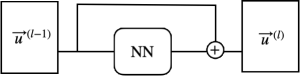
Figure 3: Calculation graph notation of Res-Net. Input and output of this component are vectors. NN in the figure indicates a neural network.

Let us derive the delta-rule called in machine-learning community with the use of the rank-2 tensor version of the backpropagation. Weight parameters in the neural networks can be tuned by minimizing a loss function with a gradient optimizer. The rank-2 local derivatives $\delta^{(l)}_{\mu}(n)$ on $l$-th layer, whose element is defined as

$$\left[\delta^{(l)}_{\mu}(n)\right]{}^{i}{}_{j}\equiv[\frac{\partial S_{\theta}}{\partial z_{\mu}^{(l)}(n)}]{}^{i}{}_{j}.$$ (7)

By introducing star-product $\star$ for rank-2 and rank-4 tensors, $\delta^{(L)}_{\mu}(n)$ on the final layer $l=L$ becomes

$$\delta^{(L)}_{\mu}(n) =\sum_{\alpha=I,II}\frac{\partial S_{\theta}}{\partial U^{(L)\alpha}_{\mu}(n)}\star\frac{\partial{\cal N}[z^{(L)}_{\mu}(n)]^{\alpha}}{\partial z^{(L)}_{\mu}(n)},$$ (8)

where $\star$ is defined in appendix, which is originally introduced in [8]. Here, we define $A^{I}(n)\equiv A$ and $A^{II}\equiv A^{\dagger}$. On the $l$-th layer, $\delta^{(l)\alpha}_{\mu}(n)$ is written as

$$\delta^{(l)}_{\mu,\alpha}(n)=\sum_{\mu^{\prime},m,\beta}\delta^{(l+1)}_{\mu^{\prime},\beta}(m)\star\frac{\partial z^{(l+1)\beta}_{\mu^{\prime}}(m)}{\partial z^{(l)\alpha}_{\mu}(n)},$$ (9)

$$=\sum_{\beta=I,II}\Bigg{\{}w_{1}^{(l)}\delta^{(l+1)}_{\mu,\beta}(n)\star\frac{\partial{\cal N}[z^{(l)\beta}_{\mu}(n)]}{\partial z^{(l)\alpha}_{\mu}(n)}$$

$$\;\;\;\;\;\;+w_{2}^{(l)}\sum_{\mu^{\prime},m}\delta^{(l+1)}_{\mu^{\prime},\beta}(m)\star\sum_{\gamma=I,II}\frac{\partial{\cal G}_{\mu^{\prime},m}(U^{(l)})^{\beta}}{\partial U^{(l)\gamma}_{\mu}(n)}\star\frac{\partial{\cal N}[z^{(l)}_{\mu}(n)]^{\gamma}}{\partial z^{(l)\alpha}_{\mu}(n)}\Bigg{\}},$$ (10)

where $\alpha,\gamma=I,II$. This is the rank-2 delta rule for the covariant neural network. And by using this delta rule, we can optimize the weights in the network through a gradient optimizer.

We can also introduce the rank-2 tensor version of the neural ODE [27], a generalization of conventional Res-Net, which is a cutting-edge framework of the deep learning [25, 26]. If the layer index $l$ is regarded as a fictitious time $t$, Eq. (6) leads the rank-2 neural ODE,

$$\frac{dU_{\mu}^{(t)}(n)}{dt} =w_{2}^{(t)}{\cal G}_{\mu,n}^{\bar{\theta}^{(t)}}(U^{(t)}).$$ (11)

Conversely, one can derive the rank-2 Res-Net (6) by solving the above differential equation with the use of the Euler method ($y_{n+1}=y_{n}+hf(t_{n},y_{n})$, for small $h$). Since a continuous version of the stout smearing [32] is known as the Wilson flow, a gradient flow with Wilson plaquette action, the flow with given parameters in lattice QCD is regarded as the neural ODE for a gauge field in terms of the machine learning technique.

III Demonstration

To show the applicability of our gauge covariant neural networks, we develop the self-learning hybrid Monte-Carlo (SLHMC) [24] for two color QCD with dynamical fermions as a demonstration.

The SLHMC is an exact algorithm developed in condensed matter community [24], which consists of two parts, the molecular dynamics and the Metropolis test. We apply the SLHMC to lattice QCD by replacing the target action $S[U]$ in molecular dynamics part in the HMC with the effective action $S_{\theta}[U]$ expressed by our gauge covariant neural networks. The exactness of the results is guaranteed by using $S[U]$ in the Metropolis test. In lattice QCD, the computational cost with dynamical fermions strongly depends on the fermion kinds and quark mass. There are several studies that expectation values of observable with numerically extensive fermions are calculated by the reweighting techniques with numerically less extensive ones [33, 34]. With the use of the SLHMC, we can employ relatively heavier fermions for generating configurations for systems with lighter ones.

In this paper, we perform SLHMC calculations with different quark mass of the staggered fermions. Our target system is written as,

$$S[U]=S_{\text{g}}[U]+S_{\text{f}}[\phi,U;m_{\text{l}}],$$ (12)

where $S_{\text{g}}[U]$ is a gauge action and $S_{\text{f}}[\phi,U;m_{\text{l}}]$ is the staggered fermion action with a psuedofermion field $\phi$ with mass $m_{\text{l}}$. We take an action for the molecular dynamics,

$$S_{\theta}[U]=S_{\text{g}}\big{[}U\big{]}+S_{\text{f}}\big{[}\phi,U^{\text{NN}}_{\theta}[U];m_{\text{h}}\big{]},$$ (13)

as an effective action. We remark that any actions with any number of parameters can be employed as an effective action as in [35].

We employ the the stout type smearing ($w_{1}^{(l)}=w_{2}^{(l)}=1$, ${\cal N}(z)=z$, and ${\cal G}_{\mu,n}(U^{(l)})=\exp(Q_{\mu}^{(l)}(n))-1$). Here, $Q_{\mu}^{(l)}(n)$ is defined as $2[\Omega_{\mu}^{(l)}(n)]_{\text{TA}}$ where TA means traceless-antihermitian operation. In the conventional stout type smearing, $\Omega^{(l)}_{\mu}(n)$ consists of untraced plaquette loop operators [3]. In the SLHMC, one can consider any kinds of closed loops operators like the HEX smearing [29]. In this paper, $\Omega^{(l)}_{\mu}(n)$ with trainable parameters is defined as

$$\Omega^{(l)}_{\mu}(n) =\rho^{(l)}_{\text{plaq}}O^{\text{plaq}}_{\mu}(n)+\begin{cases}\rho^{(l)}_{\text{poly,s}}O^{\text{poly}}_{i}(n),\;\;\text{($\mu=i=1,2,3$)},\\ \rho^{(l)}_{\text{poly,$4$}}O^{\text{poly}}_{4}(n),\;\;\text{($\mu=4$)}.\end{cases}$$ (14)

where $O^{\text{plaq}}_{\mu}(n)$, $O^{\text{poly}}_{\mu}(n)$, are plaquette, and Polyakov loop operators for $\mu$ direction originated from a point $n$, respectively. We take same weights for spatial Polyakov loops $\rho^{(l)}_{\text{poly,s}}$ from a symmetry point of view. The weights $\rho^{(l)}_{\text{plaq}},\rho^{(l)}_{\text{poly,s}},\rho^{(l)}_{\text{poly,$4$}}\in\mathbb{R}$ in the network are determined in the training. We set the number of the layers of networks to $L=2$ ($U^{\text{NN}}_{\theta}[U]=U^{(l=2)}[U^{(l=1)}[U]]$).

To train the parametrized action, we took square difference as the loss function

$$S_{\text{f}}\big{[}\phi,U^{\text{NN}}_{\theta}[U];m_{\text{h}}\big{]}-S_{\text{f}}[\phi,U;m_{\text{l}}]$$ (15)

We performed the training just after the Metropolis step in a prior run of HMC and $\phi$ is what used in the Molecular dynamics. We remark that, the training can be performed during SLHMC, but here we separately did it for simplicity.

We performed simulation for two color QCD with unrooted dynamical staggered fermions and the plaquette gauge action in $N_{\sigma}^{3}N_{\tau}=4^{4}$ with $m_{\text{l}}=0.3$ for this proof-of-principle study. The coupling is taken as $\beta=2.7$.

The SLHMC is performed with trained weights and $m_{\text{h}}=0.4$ . To increase statistics, the simulation is performed with multi-stream with different random seeds, and first 1000 trajectories for each stream are not included in the analysis. We analyze data from 50000 trajectories in total for SLHMC. Measurements for plaquette, Polyakov loop and the chiral condensate performed every trajectories. The step size in the molecular dynamics is taken to 0.02 to see quality of trained action. For HMC, we use the same number of trajectories for analysis.

III.1 Results

Here we numerically show that our effective action with gauge covariant neural networks can imitate the target action. First, we show the loss history in Fig. 6 as a function of the molecular dynamics (MD) time unit, which coincidences with the training steps. The inside plot is zoomed around MD time equals zero. The loss function starts from about 89, and after some steps, it becomes $O(1)$ with fluctuations.

Fig. 5 shows histograms of observable, plaquette and Polyakov loops, from HMC and SLHMC. Error bars are evaluated by the Jackknife method. All of the histograms are well overlapped. Tab. 1 is summary table for results from HMC and SLHMC. Autocorrelation effects in statistical error are taken into account. One can see that two algorithms give consistent results in error.

Finally, we comment on the acceptance rate of this demonstration. The value of the loss function in the early stage of the training is roughly 90, and it indicates that the acceptance rate without training is almost zero as $\mathrm{e}^{-L_{\theta}}\sim\mathrm{e}^{-90}$. It should be noted that there are only six parameters in our demonstration. We can increase the number of parameters with increasing layers, kinds of loop operators, and so on.

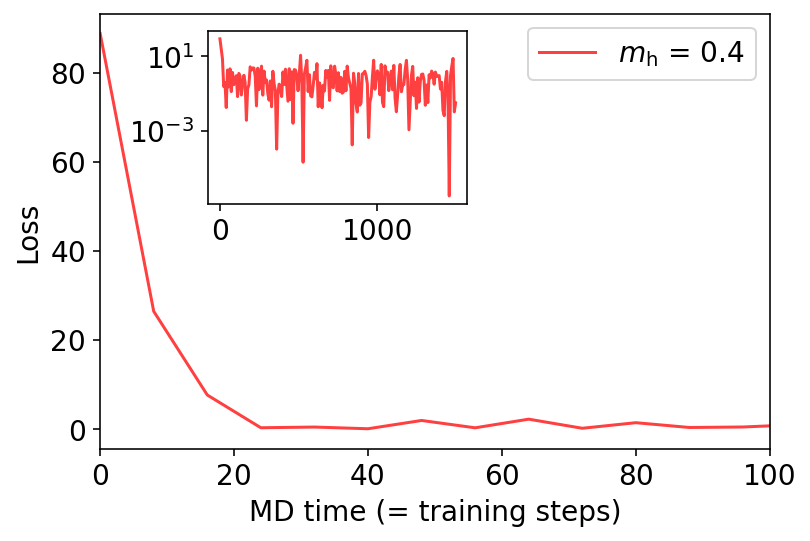
Figure 4: History of the loss function in the prior run of HMC. The horizontal axis coincides with the training steps. The inside plot is zoomed around MD time around zero in the log scale in the vertical axis.

Algorithm	Observable	Value
HMC	Plaquette	0.70257(7)
SLHMC	Plaquette	0.7024(1)
HMC	$\|\text{Polyakov loop}\|$	0.812(7)
SLHMC	$\|\text{Polyakov loop}\|$	0.824(9)
HMC	Chiral condensate	0.4245(3)
SLHMC	Chiral condensate	0.4240(3)

Table 1: Summary table for results from HMC and SLHMC.

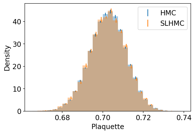
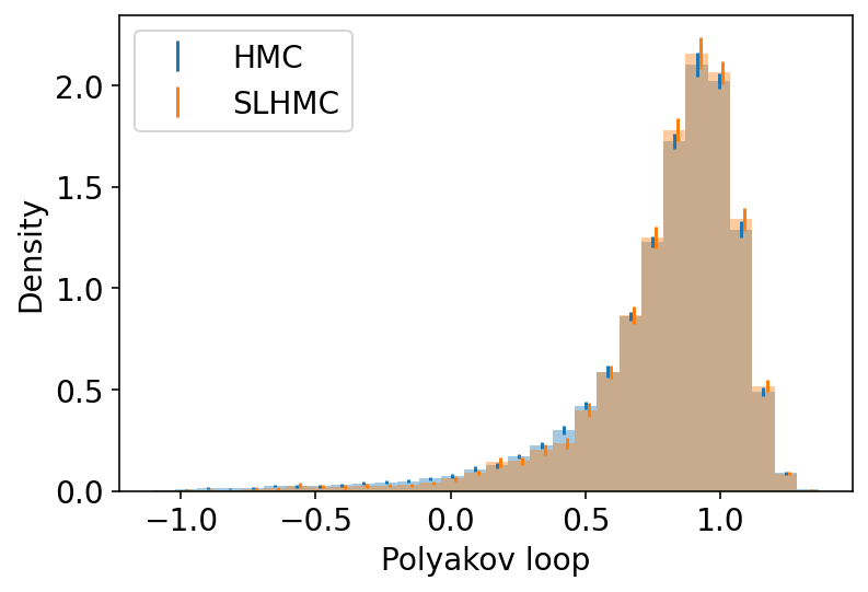
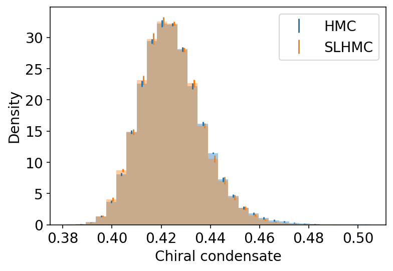
Figure 5: Comparison of results for several observables by HMC and SLHMC. Error bars for SLHMC are horizontally shifted to right to avoid overlap of symbols. (Top) plaquette, (Middle) Polyakov loop for the temporal direction. (Bottom) the chiral condensate.

IV Summary and discussion

We introduce gauge covariant neural networks, which make a map between gauge configurations with gauge covariance. Our neural networks are derived by making the parameters of the conventional smearing trainable. Using the output of the networks, we defined the real-valued gauge-invariant loss function through gauge-invariant actions. We point out that the covariant network is a rank-2 version of Res-Net and neural ODE of it has the same structure to Lüscher’s gradient flow. The covariant neural network can be trained with the rank-2 delta rule, also developed in the paper.

We apply the SLHMC [24] to lattice QCD for two-color QCD with dynamical fermions in four dimensions to show the applicability of our neural networks. The effective action with the neural networks successfully imitates the target action with dynamical fermions. We show that the results of the SLHMC are consistent with the results of the HMC.

Our network can be used for the general purpose of lattice QCD even with dynamical fermions. For example, it can be employed to simulate overlap fermions with generalized domain-wall action with tunable parameters to improve overlapping in the reweighting technique [33, 34]. By using our networks for making a map between two different probability-distribution functions, it might be helpful for the recently-developed flow-based algorithm [18, 19, 20, 21, 22]. Applications for classification problems for data with gauge symmetry would be also interesting [23, 36].

Supplemental materials

Basics of neural networks

Here we introduce conventional neural networks to be self-contained. Please refer [1] to see detail for example. Let us take $\vec{x}\in\mathbb{R}^{n}$ is an input vector of a neural network. A neural network is symbolically written as, a composite function,

$$f_{\theta}(\vec{x}) =\sigma_{L}(W_{L}\sigma_{L-1}(W_{L-1}\sigma_{L-2}(W_{L-2}\cdots\sigma_{1}(W_{1}\vec{x})\cdots))),$$ (16)

where $W_{l}\in\mathbb{R}^{n_{l+1},n_{l}}$, $l=1,2,\cdots,L$ and $\sigma_{k}(\cdot)$ ($k=1,\cdots$) is an element-wise non-linear function. We note $\theta$ as a set of parameters, namely all elements of $W_{l}$ ($l=1,\cdots,L$), which determine to minimize a loss function. Note that, including convolutional neural networks, most of known neural networks can be written in this form. It is known that, deep neural networks are universal approximator[37, 38, 39, 40], namely which can approximate any maps in desired precision as Fourier expansion in a certain order.

Let us introduce notation for later purpose. One of ingredients is a linear transformation,

$$z^{(l)}_{i}=\sum_{j}w^{(l)}_{ij}u^{(l-1)}_{j},$$ (17)

and the other is a non-linear function, ${u}^{(l)}_{i}=\sigma_{l}(z^{(l)}_{i})$. We call $z_{i}^{(l)}$ as a pre-activation variable. $w^{(l)}_{ij}$ is an element of $W_{l}$. ${u}^{(l)}_{i}$ is $i$-th component of $\vec{u}^{(l)}$ and $\vec{u}^{(0)}=\vec{x}$. Both transformation is needed to realizes a universal function from a vector space to another vector space [37, 38, 39, 40].

To determine the parameters, we use a loss function. A concrete form if the loss function is not necessary but for example for a regression we can take mean square error,

$$L_{\theta}(\mathcal{D})=\frac{1}{2|\mathcal{D}|}\sum_{(\vec{x}_{i},\vec{y}_{i})\in\mathcal{D}}(\vec{y}_{i}-f_{\theta}(\vec{x}_{i}))^{2},$$ (18)

where $\vec{y}_{i}$ is desired answer for $\vec{x}_{i}$, desired output for $\vec{x}_{i}$. $\mathcal{D}$ is a set of pairs of data, which is replaced by a part of data for mini-batch training. $|\mathcal{D}|$ is the size of data. This quantified a kind of distance between probability distribution of the answer and distribution of output. We can choose appropriate a loss function for each problem. Popular choice is the Kullback-Leibler divergence (relative entropy), the cross-entropy or the square difference[1].

A neural network is not simple convex function in general, so there are no best way to tune parameters to the optimal value. Practically, parameters in neural networks are tuned (trained) by the gradient descent,

$$\theta\leftarrow\theta-\eta\frac{\partial L_{\theta}(\mathcal{D})}{\partial\theta},$$ (19)

where $\eta$ is a real small positive number called learning rate and $\theta$ represents elements of weight matrices $W^{(l)}$. This is called stochastic gradient descent since it uses sampling approximation to evaluate the value of gradient instead of the exact expectation value. An extreme case, the size of $\mathcal{D}$ is taken to 1, it is called on-line training.

The derivative term $\frac{\partial L_{\theta}(\mathcal{D})}{\partial\theta}$, can be evaluated by a recursive formula called backpropagation and the delta rule.

$$\frac{\partial L_{\theta}(\mathcal{D})}{\partial w^{(l)}_{ij}}=\sum_{k}\frac{\partial L_{\theta}(\mathcal{D})}{\partial z^{(l)}_{k}}\frac{\partial z^{(l)}_{k}}{\partial w^{(l)}_{ij}}=\delta^{(l)}_{i}u^{(l-1)}_{j},$$ (20)

we defined,

$$\delta^{(l)}_{i}=\frac{\partial L_{\theta}(\mathcal{D})}{\partial z^{(l)}_{i}}.$$ (21)

while $z^{(l+1)}_{i}=\sum_{j}w^{(l+1)}_{ij}\sigma_{l}(z^{(l)}_{j})$, we can relate $\delta^{(l)}$ and $\delta^{(l+1)}$,

$$\delta^{(l)}_{i}=\sum_{j}\frac{\partial L_{\theta}(\mathcal{D})}{\partial z^{(l+1)}_{j}}\frac{\partial z^{(l+1)}_{j}}{\partial z^{(l)}_{i}}=\sum_{k}\delta^{(l+1)}_{k}\frac{\partial z^{(l+1)}_{k}}{\partial z^{(l)}_{i}}=\sum_{k}\delta^{(l+1)}_{k}w^{(l+1)}_{ki}\sigma^{\prime}_{l}(z^{(l)}_{i}).$$ (22)

These recursive equations enables us to calculate correction very efficiently. The information propagates $\vec{x}=\vec{u}^{(1)}\to\vec{u}^{(2)}\to\cdots\to\vec{u}^{(L)}$. The correction propagate backwards,

$$\vec{\delta}^{(1)}\leftarrow\vec{\delta}^{(2)}\leftarrow\cdots\leftarrow\vec{\delta}^{(L)},$$ (23)

where $\vec{\delta}^{(l)}$ has $\delta^{(l)}_{k}$ as elements. This is called backpropagation or backprop in short because error propagates backwards.

Gauge covariance on the lattice

Here we briefly introduce concept of gauge covariance. A link variable is defined on a bond on a lattice, which is a matrix valued function. A gauge link defined on a point $n$ with a direction $\mu$ is transformed like,

$$U_{\mu}(n)\to G(n)U_{\mu}(n)G^{\dagger}(n+\hat{\mu}).$$ (24)

where $G(n)$ is a SU(N) or U(1) valued function. This transformation law uses different element for each lattice point and it is a local symmetry. In addition, this transformation of gauge link involves two of transformation matrix $G(n)$ and $G^{\dagger}(n+\hat{\mu})$. This is not invariance but rather called covariance.

We can make a Wilson line which obeys same transformation rule with the link. For example,

$$W_{\mu}(n)=U_{\nu}(n)U_{\mu}(n+\hat{\nu})U^{\dagger}_{\nu}(n+\hat{\mu})\to G(n)W_{\mu}(n)G^{\dagger}(n+\hat{\mu}).$$ (25)

By using covariant operators, we can construct invariant objects using hermitian conjugate $\dagger$ operation and trace. For example, one non-trivial invariant object a plaquette is given,

$$\operatorname{tr}[U_{\mu}(n)W^{\dagger}_{\mu}(n)]$$ (26)

and it is transforms like,

$$\operatorname{tr}[U_{\mu}(n)W^{\dagger}_{\mu}(n)]\to\operatorname{tr}[G(n)U_{\mu}(n)G^{\dagger}(n+\hat{\mu})G(n+\hat{\mu})W^{\dagger}_{\mu}(n)G^{\dagger}(n)]=\operatorname{tr}[U_{\mu}(n)W^{\dagger}_{\mu}(n)]$$ (27)

By construction, traced loop operators are invariant because transformation matrices are canceled.

Connection to smearing

In this subsection, we identify relation between the covariant neural network and smearing schemes.

Connection to APE and n-HYP smearing

For APE-type smearing [7, 9], the parameters and functions are taken as,

$$w_{1}^{(l)} =\alpha,\;\;w_{2}^{(l)}=\frac{\alpha}{6}$$ (28)

$${\cal G}_{\mu,n}(U^{(l)}) =V_{\mu}^{\dagger(l)}[U](n)$$ (29)

where ${\cal N}(z)$ is a normalization function, which guarantees output of the layer is an element of the gauge group (or U(1) extended one with the normalization function). To express n-HYP, ${\cal N}(z)$ has to be taken to a projection function and coefficients be taken to appropriate ones. $V_{\mu}^{\dagger(l)}[U](n)$ is a staple.

Connection to stout smearing

Smearing step in the stout smearing [3] is expressed as

$$U_{\mu}^{(l+1)}(n) =\exp(Q_{\mu}^{(l)}(n))U_{\mu}^{(l)}(n)$$ (30)

$$=U_{\mu}^{(l)}(n)+\left(\exp(Q_{\mu}^{(l)}(n))-1\right)U_{\mu}^{(l)}(n).$$ (31)

So, we can identify,

$$w_{1}^{(l)} =w_{2}^{(l)}=1$$ (32)

$${\cal N}(z) =z$$ (33)

$${\cal G}_{\mu,n}(U^{(l)}) =\left(\exp(Q_{\mu}^{(l)}(n))-1\right)U_{\mu}^{(l)}(n)$$ (34)

where $Q_{\mu}^{(l)}(n)$ is defined as

$$Q_{\mu}^{(l)}(n)=2[\Omega_{\mu}^{(l)}(n)]_{\text{TA}}$$ (35)

and $\Omega_{\mu}^{(l)}(n)$ is constracted by untraced plaquette. Here TA means traceless-antihermitian operation.

Throughout this paper, we call the covariant neural network with Eq.  (29) as APE-type neural network, and with Eq.  (32) (33) (34) (35) as stout-type neural network. As we will discuss later, the stout-type neural network can contain trainable parameters in $Q_{\mu}^{(l)}(n)$.

Parametrization for stout-type covariant neural network

For stout-type covariant neural network, one has to take $w_{1}^{(l)}=w_{2}^{(l)}=1$ otherwise $\mathcal{N}$ has to take as normalization function as n-HYP. Weights can be included in $\Omega_{\mu}^{(l)}$. For example we can choose as,

$$\Omega^{(l)}_{\mu}(n)=\rho^{(l)}_{\text{plaq}}O^{\text{plaq}}_{\mu}(n)+\rho^{(l)}_{\text{rect}}O^{\text{rect}}_{\mu}(n)+\rho^{(l)}_{\text{poly}}O^{\text{poly}}_{\mu}(n),$$ (36)

where $O^{\text{plaq}}_{\mu}(n)$, $O^{\text{rect}}_{\mu}(n)$, $O^{\text{poly}}_{\mu}(n)$, are plaquette, rectangular loop, and Polyakov loop operators for $\mu$ direction originated from a point $n$, respectively. Every operators in $\Omega^{(l)}_{\mu}(n)$ is not traced as in the stout and HEX smearing [3, 29].

Connection to fully connected neural network

The covariant neural network fallback to a conventional neural network a linear function of a gauge field $A_{\mu}(n)$ if $a$ is small for $U_{\mu}(n)=\mathrm{e}^{\mathrm{i}aA_{\mu}(n)}\approx 1+\mathrm{i}aA_{\mu}(n)$. We follow the idea in [29], perturbative analysis of smearing. For example, in the APE type smearing with a staple for plaquette is,

$$w_{1}^{(l-1)}U_{\mu}(n)+w_{2}^{(l-1)}\sum_{\mu\neq\nu}[U_{\nu}(n+\hat{\mu})U^{\dagger}_{\mu}(n+\hat{\nu})U^{\dagger}_{\nu}(n)+\text{opposite}],$$ (37)

$$=w_{1}^{(l-1)}\mathrm{i}aA_{\mu}(n)+w_{2}^{(l-1)}\sum_{\mu\neq\nu}\big{[}\mathrm{i}aA_{\nu}(n+\hat{\mu})-\mathrm{i}aA_{\mu}(n+\hat{\nu})$$

$$\;\;\;-\mathrm{i}aA_{\nu}(n)+\text{(opposite)}\big{]}+\text{const}+O(a^{2}),$$ (38)

where (opposite) indicates a staple along with the opposite side. This is nothing but a linear summation of input. This is fed to an non-linear function, which corresponds to an activation function. Moreover, if we do not use weight sharing, the right hand side of equation above is extended as,

$$w_{1,\mu}^{(l-1)}(n)\mathrm{i}aA_{\mu}(n)+\sum_{\mu\neq\nu}[\mathrm{i}aw_{2,\nu}^{(l-1)}(n+\hat{\mu})A_{\nu}(n+\hat{\mu})-\mathrm{i}aw_{2,\nu}^{(l-1)}(n+\hat{\nu})A_{\mu}(n+\hat{\nu})$$

$$\;\;\;\;-\mathrm{i}aw_{2,\nu}^{(l-1)}(n)A_{\nu}(n)+\text{(opposite)}]+\text{const}+O(a^{2}).$$ (39)

If the gauge group is U(1), the gauge field $A_{\mu}(n)$ becomes real valued. This can be regarded as a dense layer in a conventional neural network if we identify a pair of index $(\mu,n)$ as index for a input vector in conventional fully connected layer.

Rank-2 back propagation

Weight parameters in a neural network can be tuned by minimizing a loss function, which can be done with a gradient optimizer. Optimization process can be symbolically written,

$$\theta\leftarrow\theta-\eta\frac{\partial L_{\theta}(\mathcal{D})}{\partial\theta},$$ (40)

where $\eta$ is a learning rate (a hyper parameter). In the calculation, we need a gradient of the loss function with respect to each weight $\frac{\partial L_{\theta}(\mathcal{D})}{\partial\theta}$. The derivatives are calculated by the delta rule and backpropagation in the machine-learning community. For example, a weight in the last layer is,

$$\frac{\partial L_{\theta}(\mathcal{D})}{\partial w^{(L-1)}_{i}}=\frac{\partial L_{\theta}(\mathcal{D})}{\partial S_{\theta}}\frac{\partial S_{\theta}}{\partial w^{(L-1)}_{i}}$$ (41)

The first factor in the right hand side is calculable if concrete form of the loss function is given while second factor requires derivative with respect to $z_{\mu}^{(L)}(n)$, which is a rank-2 object. Thus, we cannot use conventional delta rule and we have to develop a rank-2 version.

Chain rules and star product

The scalar version of the back propagation scheme is derived from so-called the delta rule. In this section, we derive the rank-2 version of the delta rule.

We introduce the matrix-valued “local” derivatives $\delta_{\mu}^{(l)}(n)$ on $l$-th layer, whose matrix element is defined as

$$[\delta_{\mu}^{(l)}(n)]^{i}{}_{j} \equiv[\frac{\partial S_{\theta}}{\partial z_{\mu}^{(l)}(n)}]^{i}{}_{j}$$ (42)

$$[\bar{\delta}_{\mu}^{(l)}(n)]^{i}{}_{j} \equiv[\frac{\partial S_{\theta}}{\partial z_{\mu}^{(l)\dagger}(n)}]^{i}{}_{j}$$ (43)

Here, we use definition of matrix derivative on a scalar function $f$ as

$$[\frac{\partial f}{\partial A}]^{i}{}_{j}\equiv\frac{\partial f}{\partial A^{j}{}_{i}}$$ (44)

as in [8]. With the use of $\delta_{\mu}^{(l)}(n)$, the derivative with respect to the parameter can be calculated with a chain rule for a matrix

$$\frac{\partial S_{\theta}}{\partial{\theta}^{(l-1)}} =\sum_{\mu,n}\sum_{ij}\frac{\partial S_{\theta}}{\partial[z_{\mu}^{(l)}(n)]^{i}{}_{j}}\frac{\partial[z_{\mu}^{(l)}(n)]^{i}{}_{j}}{\partial{\theta}^{(l-1)}}=\sum_{\mu,n}\operatorname{Tr}\left[\frac{\partial S_{\theta}}{\partial z_{\mu}^{(l)}(n)}\frac{\partial z_{\mu}^{(l)}(n)}{\partial{\theta}^{(l-1)}}\right],$$ (45)

where ${\theta}^{(l-1)}$ is a parameter in $(l-1)$-th layer. If $z_{\mu}(n)$ is a function respect to $A_{\mu,m}$, a matrix-valued derivative $\partial f/\partial z_{\mu}(n)$ can be also calculated with a chain rule

$$\frac{\partial f}{\partial z_{\mu}(n)} =\sum_{\mu^{\prime},m}\frac{\partial f}{\partial A_{\mu^{\prime},n^{\prime}}}\star\frac{\partial A_{\mu^{\prime},n^{\prime}}}{\partial z_{\mu}(n)}$$ (46)

Here, we introduce the star product for the rank-2 and rank-4 tensors defined as

$$[A\star T]^{i}{}_{j} \equiv\sum_{kl}A^{l}{}_{k}T^{k}{}_{j}{}^{i}{}_{l},$$ (47)

and the rank-4 tensor $\partial M/\partial A$ is defined as

$$[\frac{\partial M}{\partial A}]^{i}{}_{j}{}^{k}{}_{l} \equiv\frac{\partial}{\partial B^{j}{}_{k}}[M]^{i}{}_{l}$$ (48)

By introducing the star product for the rank-4 and rank-4 tensors defined as

$$(S\star T)^{i}{}_{j}{}^{k}{}_{l} =\sum_{nm}S^{i}{}_{n}{}^{m}{}_{l}T^{n}{}_{j}{}^{k}{}_{m},$$ (49)

we can use a tensor version of chain rules:

$$\frac{\partial f}{\partial A} \equiv\sum_{IJ}\frac{\partial f}{\partial B_{I}}\star\frac{\partial B_{I}}{\partial C_{J}}\star\frac{\partial C_{J}}{\partial A},$$ (50)

where $I,J$ will be identified as a coordinate and direction indices. Here we used associativity of the star product.

Rank-2 Delta rule and HMC force

HMC is the de facto standard algorithm in lattice QCD because it can deal with dynamical fermions [41]. HMC is based on the Metropolis algorithm and the molecular dynamics to obtain configurations. The molecular dynamics uses gradient of the action with respect to the gauge field, which is called HMC force. For smeared action, one has to treat smeared links as a composite function of un-smeared (= thin) links, which is calculated by the chain rule. The HMC force with the covariant neural network is defined as

$$F_{\mu,n}[U] =\left[U_{\mu}(n)\frac{\partial S[U^{(L)}]}{\partial U_{\mu}(n)}\right]_{\text{TA}}=\left[U_{\mu}(n)\delta_{\mu}^{(l=0)}(n)\right]_{\text{TA}},$$ (51)

where $U^{(L)}$ is the output from the covariant neural network and $L$ is the number of covariant layers. The HMC force can be written in $\delta_{\mu}^{(l=0)}(n)$, which is actually the same object with $\Sigma(n)$ in [3] for the stout smearing case.

With the star products and tensor version of chain rules, we can straightforwardly derive rank-2 version of the delta rule, which is a recurrence formula of $\delta_{\mu}^{(l)}(n)$. We note that there were similar derivations of HMC force with specific smearing schemes. To derive the recurrence formula of $\delta_{\mu}^{(l)}(n)$, we use the following chain rule,

$$\frac{\partial S}{\partial z_{\mu}^{(l)}(n)} =\sum_{\mu^{\prime},n^{\prime}}\left[\frac{\partial S}{\partial z_{\mu^{\prime}}^{(l+1)}(n^{\prime})}\star\frac{\partial z_{\mu^{\prime}}^{(l+1)}(n^{\prime})}{\partial z_{\mu}(n)}+\frac{\partial S}{\partial z_{\mu^{\prime}}^{(l+1)\dagger}(n^{\prime})}\star\frac{\partial z_{\mu^{\prime}}^{(l+1)\dagger}(n^{\prime})}{\partial z_{\mu}(n)}\right].$$ (52)

This is an extended Wiltinger derivative to complex matrix [8] and constraint of special unitary is taken care of.

On the final layer $l=L$, $\delta^{(L)}_{\mu}(n)$ becomes

$$\delta^{(L)}_{\mu}(n) =\sum_{\alpha=I,II}\frac{\partial S_{\theta}}{\partial U^{(L)\alpha}_{\mu}(n)}\star\frac{\partial{\cal N}[z^{(L)}_{\mu}(n)]^{\alpha}}{\partial z^{(L)}_{\mu}(n)},$$ (53)

Here, we define $A^{I}(n)\equiv A$ and $A^{II}\equiv A^{\dagger}$.

On the $l$-th layer, $\delta^{(l)\alpha}_{\mu}(n)$ is written as

$$\delta^{(l)}_{\mu,\alpha}(n)=\sum_{\mu^{\prime},m,\beta}\delta^{(l+1)}_{\mu^{\prime},\beta}(m)\star\frac{\partial z^{(l+1)\beta}_{\mu^{\prime}}(m)}{\partial z^{(l)\alpha}_{\mu}(n)},$$ (54)

$$=\sum_{\beta=I,II}\left\{w_{1}^{(l)}\delta^{(l+1)}_{\mu,\beta}(n)\star\frac{\partial{\cal N}[z^{(l)\beta}_{\mu}(n)]}{\partial z^{(l)\alpha}_{\mu}(n)}+w_{2}^{(l)}\sum_{\mu^{\prime},m}\delta^{(l+1)}_{\mu^{\prime},\beta}(m)\star\sum_{\gamma=I,II}\frac{\partial{\cal G}_{\mu^{\prime},m}(U^{(l)})^{\beta}}{\partial U^{(l)\gamma}_{\mu}(n)}\star\frac{\partial{\cal N}[z^{(l)}_{\mu}(n)]^{\gamma}}{\partial z^{(l)\alpha}_{\mu}(n)}\right\},$$ (55)

where $\alpha,\gamma=I,II$. This is the rank-2 delta rule for the covariant neural network. And by using this delta rule, we can optimize the weights in the network through a gradient optimizer.

We can derive a derivative with respect to $\rho$ using formula above,

$$\frac{\partial S}{\partial\rho^{(l)}_{i}} =2\operatorname{Re}\sum_{\mu^{\prime},m}\operatorname{tr}\left[U^{(l)\dagger}_{\mu^{\prime}}(m)\Lambda_{\mu^{\prime},m}\frac{\partial C}{\partial\rho_{i}^{(l)}}\right],$$ (56)

where $\rho_{i}^{(l)}$ is a coefficient of a loop operator type $i$ (plaquette, rectangler, Polyakov loop, etc) in the level $l$. $C$ is sum of staples for loop operators in $\Omega^{(l)}_{\mu}(n)$. $\Lambda_{\mu,m}$ is defined in [3].

Tensor calculus and star product

In this subsection we derive useful formulae based on [8] but we impose the star product match to the matrix chain rule, which enables us to derive exactly the same formula in [3] with the star product formulation.

Definition of matrix derivative

The derivative of a scalar $f$ function of a matrix $A$ of independent variables, with respect to the matrix $A$ is a rank-2 tensor:

$$[\frac{\partial f[A]}{\partial A}]^{i}{}_{j} \equiv\frac{\partial f}{\partial A^{j}{}_{i}}.$$ (57)

The derivative of a matrix $M$ function of a matrix $A$ of independent variables, with respect to the matrix $A$ is a rank-4 tensor:

$$[\frac{\partial M[A]}{\partial A}]^{i}{}_{j}{}^{k}{}_{l} \equiv\frac{\partial}{\partial A^{j}{}_{k}}M[A]^{i}{}_{l}$$ (58)

This is matrix-generalized Wirtinger derivative and for derivative with a complex number, it is fall back to conventional Wirtinger derivative. The derivative of a matrix $M$ function of a scalar $x$ of independent variables, with respect to the matrix $x$ is a rank-2 tensor:

$$[\frac{\partial M[x]}{\partial x}]^{i}{}_{j} \equiv\frac{\partial M[x]^{i}{}_{j}}{\partial x}.$$ (59)

Chain rules and star products

The chain rule is given as

$$[\frac{\partial f[A]}{\partial A}]^{i}{}_{j} =\frac{\partial f}{\partial A^{j}{}_{i}}=\sum_{kl}\frac{\partial f}{\partial B^{k}{}_{l}}\frac{\partial B^{k}{}_{l}}{\partial A^{j}{}_{i}}$$ (60)

$$=\sum_{kl}[\frac{\partial f}{\partial B}]^{l}{}_{k}[\frac{\partial B}{\partial A}]^{k}{}_{j}{}^{i}{}_{l}$$ (61)

Then, by defining rank-2-rank4 “star”-product

$$[A\star T]^{i}{}_{j} \equiv\sum_{kl}A^{l}{}_{k}T^{k}{}_{j}{}^{i}{}_{l},$$ (62)

we have

$$\frac{\partial f}{\partial A} =\frac{\partial f}{\partial B}\star\frac{\partial B}{\partial A}$$ (63)

We consider the following chain rule:

$$[\frac{\partial M[A]}{\partial A}]^{i}{}_{j}{}^{k}{}_{l} =\sum_{nm}\frac{\partial M[A]^{i}{}_{l}}{\partial B^{n}{}_{m}}\frac{\partial B^{n}{}_{m}}{\partial A^{j}{}_{k}}$$ (64)

$$=\sum_{nm}[\frac{\partial M[B]}{\partial B}]^{i}{}_{n}{}^{m}{}_{l}[\frac{\partial B[A]}{\partial A}]^{n}{}_{j}{}^{k}{}_{m}$$ (65)

By defining rank-4-rank4 star product:

$$(S\star T)^{i}{}_{j}{}^{k}{}_{l} =\sum_{nm}S^{i}{}_{n}{}^{m}{}_{l}T^{n}{}_{j}{}^{k}{}_{m}$$ (66)

we have

$$\frac{\partial M[A]}{\partial A} =\frac{\partial M[B]}{\partial B}\star\frac{\partial B[A]}{\partial A}$$ (67)

We consider a different chain rule:

$$\frac{\partial f}{\partial x} =\sum_{ij}\frac{\partial f}{\partial A^{j}{}_{i}}\frac{\partial A^{j}_{i}}{\partial x}$$ (68)

$$=\sum_{ij}\left[\frac{\partial f}{\partial A}\right]^{i}{}_{j}\left[\frac{\partial A}{\partial x}\right]^{j}{}_{i}$$ (69)

$$={\rm Tr}\left[\left[\frac{\partial f}{\partial A}\right]\left[\frac{\partial A}{\partial x}\right]\right]$$ (70)

Here, $f$ and $x$ are scalars. We can define a rank-2-rank-2 star product.

$$A\star B \equiv{\rm Tr}\left[AB\right]$$ (71)

And we have

$$\frac{\partial f}{\partial x} =\sum_{ij}\frac{\partial f}{\partial A^{j}{}_{i}}\frac{\partial A^{j}_{i}}{\partial x}$$ (72)

$$=\sum_{ij}\sum_{kl}\frac{\partial f}{\partial B^{k}{}_{l}}\frac{\partial B^{k}{}_{l}}{\partial A^{j}_{i}}\frac{\partial A^{j}_{i}}{\partial x}$$ (73)

$$=\sum_{ij}\sum_{kl}[\frac{\partial f}{\partial B}]{}^{l}{}_{k}[\frac{\partial B}{\partial A}]{}^{k}{}_{i}{}^{j}{}_{l}[\frac{\partial A}{\partial x}]{}^{i}{}_{j}$$ (74)

$$=\sum_{ij}\sum_{kl}[\frac{\partial f}{\partial B}]{}^{l}{}_{k}[\frac{\partial B}{\partial A}\star\frac{\partial A}{\partial x}]{}^{k}{}_{l}$$ (75)

$$=\frac{\partial f}{\partial B}\star(\frac{\partial B}{\partial A}\star\frac{\partial A}{\partial x})$$ (76)

Here we use the following definition:

$$[S\star A]^{i}{}_{j} \equiv S^{i}{}_{k}{}^{l}{}_{j}A^{k}{}_{l}$$ (77)

This is a definition of a rank-4-rank-2 star product.

Product rules

We consider the following product rule:

$$[\frac{\partial(f[A]M[A])}{\partial A}]^{i}{}_{j}{}^{k}{}_{l} =\frac{\partial}{\partial A^{j}{}_{k}}(f[A]M[A]^{i}{}_{l}])$$ (78)

$$=\frac{\partial f[A]}{\partial A^{j}{}_{k}}M[A]^{i}{}_{l}+f[A]\frac{\partial}{\partial A^{j}{}_{k}}M[A]^{i}{}_{l}$$ (79)

$$=[\frac{\partial f[A]}{\partial A}]^{k}{}_{j}M[A]^{i}{}_{l}+f[A][\frac{\partial M[A]}{\partial A}]^{i}{}_{j}{}^{k}{}_{l}$$ (80)

By defining “direct” product:

$$(A\oplus B)^{i}{}_{j}{}^{k}{}_{l} =A^{k}{}_{j}B^{i}{}_{l}$$ (81)

we have

$$\frac{\partial f[A]M[A]}{\partial A} =\frac{\partial f[A]}{\partial A}\oplus M[A]+f[A]\frac{\partial M[A]}{\partial A}$$ (82)

We consider the matrix $M=ABC$. The derivative is

$$[\frac{\partial M[B]}{\partial B}]^{i}{}_{j}{}^{k}{}_{l} =\frac{\partial}{\partial B^{j}{}_{k}}M[B]^{i}{}_{l}$$ (83)

$$=\sum_{n,m}\frac{\partial}{\partial B^{j}{}_{k}}(A^{i}{}_{n}B^{n}_{m}C^{m}_{l})$$ (84)

$$\sum_{n,m}(A^{i}{}_{n}\delta_{jn}\delta_{km}C^{m}_{l})$$ (85)

$$=A^{i}{}_{j}C^{k}_{l}$$ (86)

By defining the outer product

$$(A\otimes B)^{i}{}_{j}{}^{k}{}_{l} \equiv A^{i}{}_{j}B^{k}_{l}$$ (87)

we have

$$\frac{\partial M[B]}{\partial B} =A\otimes C$$ (88)

We consider

$$[\frac{\partial(Y[A]Z[A])}{\partial A}]^{i}{}_{j}{}^{k}{}_{l} =\frac{\partial}{\partial A^{j}{}_{k}}[YZ]^{i}{}_{l}$$ (89)

$$=\sum_{n}\frac{\partial}{\partial A^{j}{}_{k}}(Y^{i}{}_{n}Z^{n}{}_{l})$$ (90)

$$=\sum_{n}\frac{\partial Y^{i}{}_{n}}{\partial A^{j}{}_{k}}Z^{n}{}_{l}+\sum_{n}Y^{i}{}_{n}\frac{\partial Z^{n}{}_{l}}{\partial A^{j}{}_{k}}$$ (91)

$$=\sum_{n}[\frac{\partial Y[A]}{\partial A}]^{i}{}_{j}{}^{k}{}_{n}Z^{n}{}_{l}+\sum_{n}Y^{i}{}_{n}[\frac{\partial Z[A]}{\partial A}]^{n}{}_{j}{}^{k}{}_{l}$$ (92)

By defining the contraction:

$$[AT]^{i}{}_{j}{}^{k}{}_{l} =\sum_{n}A^{i}{}_{n}T^{n}{}_{j}{}^{k}{}_{l}$$ (93)

$$[TA]^{i}{}_{j}{}^{k}{}_{l} =\sum_{n}T^{i}{}_{j}{}^{k}{}_{n}A^{n}{}_{l}$$ (94)

we have

$$\frac{\partial YZ}{\partial A} =\frac{\partial Y[A]}{\partial A}Z+Y\frac{\partial Z[A]}{\partial A}$$ (95)

Useful formulas

The useful formulas are given as

$$\frac{\partial A}{\partial A} =I\otimes I$$ (96)

$$A\star(B\oplus C) ={\rm Tr}(AC)B$$ (97)

$$A\star(B\otimes C) =CAB$$ (98)

$$(A\otimes B)\star(C\otimes D) =(AC)\otimes(DB)$$ (99)

$$(A\oplus B)\star(C\oplus D) ={\rm Tr}(AD)(C\oplus B)$$ (100)

$$(A\otimes B)\star(C\oplus D) =C\oplus(ADB)$$ (101)

$$(A\oplus B)\star(C\otimes D) =(DAC)\oplus B$$ (102)

$$S\star(T\star K) =(S\star T)\star K$$ (103)

$$A\star(T\star K) =(A\star T)\star K$$ (104)

$$(A\otimes B)C =A\otimes(BC)$$ (105)

$$(A\oplus B)C =A\oplus(BC)$$ (106)

$$C(A\otimes B) =(CA)\otimes B$$ (107)

$$C(A\oplus B) =A\oplus(CB)$$ (108)

$$(S\star T)C =(SC)\star T$$ (109)

$$A\star(TC) =(CA)\star T$$ (110)

$$S\star(I\otimes I) =S$$ (111)

$$B^{\dagger}\star\frac{\partial M^{\dagger}}{\partial A^{\dagger}} =[B\star\frac{\partial M}{\partial A}]^{\dagger}$$ (112)

Backpropagation for stout smearing

Definition

Smearing step in the stout smearing [3] is expressed as

$$U_{\mu}^{(l+1)}(n) =\exp(Q_{\mu}^{(l)}(n))U_{\mu}^{(l)}(n)$$ (113)

$$=U_{\mu}^{(l)}(n)+\left(\exp(Q_{\mu}^{(l)}(n))-1\right)U_{\mu}^{(l)}(n).$$ (114)

So, we can identify,

$$w_{1}^{(l)} =w_{2}^{(l)}=1$$ (115)

$${\cal N}(z) =z$$ (116)

$${\cal G}_{\mu,n}(U^{(l)}) =\left(\exp(Q_{\mu}^{(l)}(n))-1\right)U_{\mu}^{(l)}(n)$$ (117)

where $Q_{\mu}^{l}(n)$ and

$$Q_{\mu}(n) =-\frac{1}{2}(\Omega_{\mu}(n)-\Omega_{\mu}^{\dagger}(n))+\frac{1}{2N}\operatorname{Tr}(\Omega_{\mu}^{\dagger}(n)-\Omega_{\mu}(n))$$ (118)

$$\Omega_{\mu}(n) =C_{\mu}(n)U_{\mu}^{\dagger}(n)$$ (119)

and $C_{\mu}(n)$ is the weighted sum of the perpendicular staples which begin at lattice site $n$ and terminate at neighboring site $n+\hat{\mu}$. For example, the staple of a plaquette loop is given as

$$\sum_{\nu\neq\mu}\rho_{\mu,\nu}\left(U_{\nu}(n)U_{\mu}(n+\hat{\nu})U_{\nu}^{\dagger}(n+\hat{\mu})+U_{\nu}^{\dagger}(n-\hat{\nu})U_{\mu}(x-\nu)U_{\nu}(x-\hat{\nu}+\hat{\mu})\right)$$ (120)

Backpropagation

In the stout smearing scheme, the $\delta_{\mu}(n)$ is given as

$$\delta_{\mu}^{(l)}(n) =\frac{\partial S}{\partial z_{\mu}^{(l)}(n)}=\frac{\partial S}{\partial U_{\mu}^{(l)}(n)}$$ (121)

$$\bar{\delta}_{\mu}^{(l)}(n) =\frac{\partial S}{\partial U_{\mu}^{(l)\dagger}(n)}=\frac{\partial S}{\partial U_{\mu}^{(l)}(n)}\star\frac{\partial U_{\mu}^{(l)}(n)}{\partial U_{\mu}^{(l)\dagger}(n)}$$ (122)

$$=\frac{\partial S}{\partial U_{\mu}^{(l)}(n)}\star\frac{\partial(U_{\mu}^{(l)\dagger}(n))^{-1}}{\partial U_{\mu}^{(l)\dagger}(n)}$$ (123)

$$=-\frac{\partial S}{\partial U_{\mu}^{(l)}(n)}\star(U_{\mu}^{(l)}(n)\otimes U_{\mu}^{(l)(n))})$$ (124)

$$=-U_{\mu}^{(l)}(n)\delta_{\mu}^{(l)}(n)U_{\mu}^{(l)}(n)$$ (125)

On the $l$-th layer, the backpropagation is given as

$$\delta^{(l)}_{\mu}(n)=\delta^{(l+1)}_{\mu}(n)\star(I\otimes I)$$

$$+\sum_{\mu^{\prime},m}\delta^{(l+1)}_{\mu^{\prime}}(m)\star\left[\frac{\partial{\cal G}_{\mu^{\prime},m}(U^{(l)})}{\partial U^{(l)}_{\mu}(n)}\star(I\otimes I)\right]-\sum_{\mu^{\prime},m}(U_{\mu^{\prime},m}\delta^{(l+1)}_{\mu^{\prime}}(m)U_{\mu^{\prime},m})\star\left[\frac{\partial{\cal G}_{\mu^{\prime},m}(U^{(l)})^{\dagger}}{\partial U^{(l)}_{\mu}(n)}\star(I\otimes I)\right]$$

By substituting

$$\frac{\partial{\cal G}_{\mu^{\prime},m}(U^{(l)})}{\partial U^{(l)}_{\mu}(n)} =\frac{\partial\exp(Q_{\mu^{\prime}}^{(l)}(m))}{\partial U^{(l)}_{\mu}(n)}U_{\mu^{\prime}}^{(l)}(m)+(\exp(Q_{\mu^{\prime}}^{(l)}(m))-I)\frac{\partial U_{\mu^{\prime}}^{(l)}(m)}{\partial U^{(l)}_{\mu}(n)}$$ (126)

$$=\frac{\partial\exp(Q_{\mu^{\prime}}^{(l)}(m))}{\partial U^{(l)}_{\mu}(n)}U_{\mu^{\prime}}^{(l)}(m)+(\exp(Q_{\mu^{\prime}}^{(l)}(m))-I)\delta_{\mu,\mu^{\prime}}\delta_{n,m}I\otimes I$$ (127)

$$\frac{\partial{\cal G}_{\mu^{\prime},m}^{\dagger}(U^{(l)})}{\partial U^{(l)}_{\mu}(n)} =U_{\mu^{\prime}}^{(l)\dagger}(m)\frac{\partial\exp(Q_{\mu^{\prime}}^{(l)\dagger}(m))}{\partial U^{(l)}_{\mu}(n)}$$ (128)

we have

$$\delta^{(l)}_{\mu}(n)=\delta^{(l+1)}_{\mu}(n))\exp(Q_{\mu^{\prime}}^{(l)}(m))\star(I\otimes I)$$

$$+\sum_{\mu^{\prime},m}(U_{\mu^{\prime}}^{(l)}(m)\delta^{(l+1)}_{\mu^{\prime}}(m))\star\frac{\partial\exp(Q_{\mu^{\prime}}^{(l)}(m))}{\partial U^{(l)}_{\mu}(n)}\star(I\otimes I)$$

$$-\sum_{\mu^{\prime},m}(\delta^{(l+1)\dagger}_{\mu^{\prime}}(m)U_{\mu^{\prime}}^{(l)\dagger}(m))\star\left[-\frac{\partial\exp(Q_{\mu^{\prime}}^{(l)\dagger}(m))}{\partial U^{(l)}_{\mu}(n)}\right]\star(I\otimes I)$$ (129)

Here we use $\delta=-U^{\dagger}\delta^{\dagger}U^{\dagger}$.

The exponentials are given as

$$\frac{\partial\exp(Q_{\mu^{\prime}}^{(l)}(m))}{\partial U^{(l)}_{\mu}(n)} =\frac{\partial\exp(Q_{\mu^{\prime}}^{(l)}(m))}{\partial Q^{(l)}_{\mu^{\prime}}(m)}\star\frac{\partial Q^{(l)}_{\mu^{\prime}}(m)}{\partial U^{(l)}_{\mu}(n)}$$ (130)

$$=\frac{\partial\exp(Q_{\mu^{\prime}}^{(l)}(m))}{\partial Q^{(l)}_{\mu^{\prime}}(m)}\star\left[\frac{\partial Q^{(l)}_{\mu^{\prime}}(m)}{\partial\Omega^{(l)}_{\mu}(n)}\star\frac{\partial\Omega^{(l)}_{\mu^{\prime}}(m)}{\partial U^{(l)}_{\mu}(n)}+\frac{\partial Q^{(l)}_{\mu^{\prime}}(m)}{\partial\Omega^{(l)\dagger}_{\mu}(n)}\star\frac{\partial\Omega^{(l)\dagger}_{\mu^{\prime}}(m)}{\partial U^{(l)}_{\mu}(n)}\right]$$ (131)

$$=\frac{\partial\exp(Q_{\mu^{\prime}}^{(l)}(m))}{\partial Q^{(l)}_{\mu^{\prime}}(m)}\star\frac{\partial Q^{(l)}_{\mu^{\prime}}(m)}{\partial\Omega^{(l)}_{\mu}(n)}\star\left[\frac{\partial\Omega^{(l)}_{\mu^{\prime}}(m)}{\partial U^{(l)}_{\mu}(n)}-\frac{\partial\Omega^{(l)\dagger}_{\mu^{\prime}}(m)}{\partial U^{(l)}_{\mu}(n)}\right]$$ (132)

and

$$\frac{\partial\exp(Q_{\mu^{\prime}}^{(l)\dagger}(m))}{\partial U^{(l)}_{\mu}(n)} =\frac{\partial\exp(Q_{\mu^{\prime}}^{(l)\dagger}(m))}{\partial Q^{(l)\dagger}_{\mu^{\prime}}(m)}\star\frac{\partial Q^{(l)\dagger}_{\mu^{\prime}}(m)}{\partial\Omega^{(l)}_{\mu}(n)}\star\left[\frac{\partial\Omega^{(l)}_{\mu^{\prime}}(m)}{\partial U^{(l)}_{\mu}(n)}-\frac{\partial\Omega^{(l)\dagger}_{\mu^{\prime}}(m)}{\partial U^{(l)}_{\mu}(n)}\right]$$ (133)

By using the fact that $Q^{(l)}$ is a traceless anti-hermitian matrix, we have

$$\frac{\partial Q^{(l)\dagger}_{\mu^{\prime}}(m)}{\partial\Omega^{(l)}_{\mu}(n)} =-\frac{\partial Q^{(l)}_{\mu^{\prime}}(m)}{\partial\Omega^{(l)}_{\mu}(n)}$$ (134)

Thus, the equations can be expressed as

$$\delta^{(l)}_{\mu}(n)=\delta^{(l+1)}_{\mu}(n)\exp(Q_{\mu^{\prime}}^{(l)}(m))\star(I\otimes I)$$

$$+\sum_{\mu^{\prime},m}(U_{\mu^{\prime}}^{(l)}(m)\delta^{(l+1)}_{\mu^{\prime}}(m))\star\frac{\partial\exp(Q_{\mu^{\prime}}^{(l)}(m))}{\partial Q^{(l)}_{\mu^{\prime}}(m)}\star\frac{\partial Q^{(l)}_{\mu^{\prime}}(m)}{\partial\Omega^{(l)}_{\mu}(n)}\star\left[\frac{\partial\Omega^{(l)}_{\mu^{\prime}}(m)}{\partial U^{(l)}_{\mu}(n)}-\frac{\partial\Omega^{(l)\dagger}_{\mu^{\prime}}(m)}{\partial U^{(l)}_{\mu}(n)}\right]\star(I\otimes I)$$

$$-\sum_{\mu^{\prime},m}(U_{\mu^{\prime}}^{(l)}(m)\delta^{(l+1)}_{\mu^{\prime}}(m))^{\dagger}\star\frac{\partial\exp(Q_{\mu^{\prime}}^{(l)\dagger}(m))}{\partial Q^{(l)\dagger}_{\mu^{\prime}}(m)}\star\frac{\partial Q^{(l)}_{\mu^{\prime}}(m)}{\partial\Omega^{(l)}_{\mu}(n)}\star\left[\frac{\partial\Omega^{(l)}_{\mu^{\prime}}(m)}{\partial U^{(l)}_{\mu}(n)}-\frac{\partial\Omega^{(l)\dagger}_{\mu^{\prime}}(m)}{\partial U^{(l)}_{\mu}(n)}\right]\star(I\otimes I)$$ (135)

$$=\delta^{(l+1)}_{\mu}(n)\exp(Q_{\mu^{\prime}}^{(l)}(m))\star(I\otimes I)$$

$$+\sum_{\mu^{\prime},m}(M_{\mu^{\prime},m}-M_{\mu^{\prime},m}^{\dagger})\star\frac{\partial Q^{(l)}_{\mu^{\prime}}(m)}{\partial\Omega^{(l)}_{\mu}(n)}\star\left[\frac{\partial\Omega^{(l)}_{\mu^{\prime}}(m)}{\partial U^{(l)}_{\mu}(n)}-\frac{\partial\Omega^{(l)\dagger}_{\mu^{\prime}}(m)}{\partial U^{(l)}_{\mu}(n)}\right]\star(I\otimes I),$$ (136)

$$M_{\mu^{\prime},m}\equiv(U_{\mu^{\prime}}^{(l)}(m)\delta^{(l+1)}_{\mu^{\prime}}(m))\star\frac{\partial\exp(Q_{\mu^{\prime}}^{(l)}(m))}{\partial Q^{(l)}_{\mu^{\prime}}(m)}$$ (137)

By using the following equation:

$$\frac{\partial Q_{\mu}(y)}{\partial\Omega_{\mu}(y)} =-\frac{\partial}{\partial\Omega_{\mu}(y)}\left[\frac{1}{2}\left[\Omega_{\mu}(y)^{\dagger}-\Omega_{\mu}(y)\right]-\frac{1}{2N}{\rm Tr}\Omega_{\mu}(y)^{\dagger}I+\frac{1}{2N}{\rm Tr}\Omega_{\mu}(y)I\right]$$ (138)

$$=\frac{1}{2}\frac{\partial\Omega_{\mu}(y)}{\partial\Omega_{\mu}(y)}-\frac{1}{2N}\frac{\partial{\rm Tr}\Omega_{\mu}(y)}{\partial\Omega_{\mu}(y)}\oplus I$$ (139)

$$=\frac{1}{2}I\otimes I-\frac{1}{2N}I\oplus I$$ (140)

and the following formula

$$A\star(\frac{1}{2}I\otimes I-\frac{1}{2N}I\oplus I) =\frac{1}{2}A\star(I\otimes I)-\frac{1}{2N}A\star(I\oplus I)$$ (141)

$$=\frac{1}{2}A-\frac{1}{2N}{\rm Tr}(A)I$$ (142)

we obtain

$$\delta^{(l)}_{\mu}(n)=\delta^{(l+1)}_{\mu}(n)\exp(Q_{\mu^{\prime}}^{(l)}(m))\star(I\otimes I)$$

$$+\sum_{\mu^{\prime},m}\Lambda_{\mu^{\prime},m}\star\left[\frac{\partial\Omega^{(l)}_{\mu^{\prime}}(m)}{\partial U^{(l)}_{\mu}(n)}-\frac{\partial\Omega^{(l)\dagger}_{\mu^{\prime}}(m)}{\partial U^{(l)}_{\mu}(n)}\right]\star(I\otimes I)$$ (143)

$$=\delta^{(l+1)}_{\mu}(n)\exp(Q_{\mu^{\prime}}^{(l)}(m))+\sum_{\mu^{\prime},m}\Lambda_{\mu^{\prime},m}\star\left[\frac{\partial\Omega^{(l)}_{\mu^{\prime}}(m)}{\partial U^{(l)}_{\mu}(n)}-\frac{\partial\Omega^{(l)\dagger}_{\mu^{\prime}}(m)}{\partial U^{(l)}_{\mu}(n)}\right]$$ (144)

Here, $\Lambda_{\mu,n}$ is defined as

$$\Lambda_{\mu^{\prime},m} \equiv\frac{1}{2}(M_{\mu^{\prime},m}-M_{\mu^{\prime},m}^{\dagger})-\frac{1}{2N}{\rm Tr}(M_{\mu^{\prime},m}-M_{\mu^{\prime},m}^{\dagger})I$$ (145)

With the use of the following equations:

$$\frac{\partial\Omega^{(l)}_{\mu^{\prime}}(m)}{\partial U^{(l)}_{\mu}(n)} =\frac{\partial(C_{\mu^{\prime},m}U_{\mu^{\prime}}^{\dagger}(m))}{\partial U^{(l)}_{\mu}(n)}=\frac{\partial C_{\mu^{\prime},m}}{\partial U^{(l)}_{\mu}(n)}U^{(l)\dagger}_{\mu^{\prime}}(m)$$ (146)

$$\frac{\partial\Omega^{(l)\dagger}_{\mu^{\prime}}(m)}{\partial U^{(l)}_{\mu}(n)} =\frac{\partial(U_{\mu^{\prime}}(m)C_{\mu^{\prime},m}^{\dagger})}{\partial U^{(l)}_{\mu}(n)}=U_{\mu^{\prime}}(m)\frac{\partial C_{\mu^{\prime},m}^{\dagger}}{\partial U^{(l)}_{\mu}(n)}+\frac{\partial U_{\mu^{\prime}}(m)}{\partial U^{(l)}_{\mu}(n)}C_{\mu^{\prime},m}^{\dagger}$$ (147)

$$=U_{\mu^{\prime}}(m)\frac{\partial C_{\mu^{\prime},m}^{\dagger}}{\partial U^{(l)}_{\mu}(n)}+\delta_{\mu,\mu^{\prime}}\delta_{n,m}I\otimes IC_{\mu,n}^{\dagger}$$ (148)

$$=U_{\mu^{\prime}}(m)\frac{\partial C_{\mu^{\prime},m}^{\dagger}}{\partial U^{(l)}_{\mu}(n)}+\delta_{\mu,\mu^{\prime}}\delta_{n,m}I\otimes C_{\mu,n}^{\dagger}$$ (149)

$$\frac{\partial\Omega^{(l)}_{\mu^{\prime}}(m)}{\partial U^{(l)}_{\mu}(n)}-\frac{\partial\Omega^{(l)\dagger}_{\mu^{\prime}}(m)}{\partial U^{(l)}_{\mu}(n)} =\frac{\partial C_{\mu^{\prime},m}}{\partial U^{(l)}_{\mu}(n)}U^{(l)\dagger}_{\mu}(n)-U_{\mu^{\prime}}(m)\frac{\partial C_{\mu^{\prime},m}^{\dagger}}{\partial U^{(l)}_{\mu}(n)}-\delta_{\mu,\mu^{\prime}}\delta_{n,m}I\otimes C_{\mu,n}^{\dagger}$$ (150)

We finally obtain

$$\delta^{(l)}_{\mu}(n)=\delta^{(l+1)}_{\mu}(n)\exp(Q_{\mu^{\prime}}^{(l)}(m))-\Lambda_{\mu,n}\star(I\otimes C_{\mu,n}^{\dagger})$$

$$+\sum_{\mu^{\prime},m}\Lambda_{\mu^{\prime},m}\star\left[\frac{\partial C_{\mu^{\prime},m}}{\partial U^{(l)}_{\mu}(n)}U^{(l)\dagger}_{\mu^{\prime}}(m)-U_{\mu^{\prime}}(m)\frac{\partial C_{\mu^{\prime},m}^{\dagger}}{\partial U^{(l)}_{\mu}(n)}\right]$$ (151)

$$=\delta^{(l+1)}_{\mu}(n)\exp(Q_{\mu^{\prime}}^{(l)}(m))-C_{\mu,n}^{\dagger}\Lambda_{\mu,n}$$

$$+\sum_{\mu^{\prime},m}\Lambda_{\mu^{\prime},m}\star\left[\frac{\partial C_{\mu^{\prime},m}}{\partial U^{(l)}_{\mu}(n)}U^{(l)\dagger}_{\mu^{\prime}}(m)-U_{\mu^{\prime}}(m)\frac{\partial C_{\mu^{\prime},m}^{\dagger}}{\partial U^{(l)}_{\mu}(n)}\right]$$ (152)

$$=\delta^{(l+1)}_{\mu}(n)\exp(Q_{\mu^{\prime}}^{(l)}(m))-C_{\mu,n}^{\dagger}\Lambda_{\mu,n}$$

$$+\sum_{\mu^{\prime},m}\left[(U^{(l)\dagger}_{\mu^{\prime}}(m)\Lambda_{\mu^{\prime},m})\star\frac{\partial C_{\mu^{\prime},m}}{\partial U^{(l)}_{\mu}(n)}-(\Lambda_{\mu^{\prime},m}U_{\mu^{\prime}}(m))\star\frac{\partial C_{\mu^{\prime},m}^{\dagger}}{\partial U^{(l)}_{\mu}(n)}\right]$$ (153)

$$=\delta^{(l+1)}_{\mu}(n)\exp(Q_{\mu^{\prime}}^{(l)}(m))-C_{\mu,n}^{\dagger}\Lambda_{\mu,n}$$

$$+\sum_{\mu^{\prime},m}\left[(U^{(l)\dagger}_{\mu^{\prime}}(m)\Lambda_{\mu^{\prime},m})\star\frac{\partial C_{\mu^{\prime},m}}{\partial U^{(l)}_{\mu}(n)}+(U_{\mu^{\prime}}^{\dagger}(m)\Lambda_{\mu^{\prime},m})^{\dagger}\star\frac{\partial C_{\mu^{\prime},m}^{\dagger}}{\partial U^{(l)}_{\mu}(n)}\right]$$ (154)

The above equation has only one star product. The rank-4 tensors $\frac{\partial C_{\mu^{\prime},m}}{\partial U^{(l)}_{\mu}(n)}$ and $\frac{\partial C_{\mu^{\prime},m}^{\dagger}}{\partial U^{(l)}_{\mu}(n)}$ are usually expressed as

$$\frac{\partial C_{\mu^{\prime},m}}{\partial U^{(l)}_{\mu}(n)} \equiv\sum_{i}A_{\mu,m}^{i}\otimes B_{\mu,m}^{i}$$ (155)

$$\frac{\partial C_{\mu^{\prime},m}^{\dagger}}{\partial U^{(l)}_{\mu}(n)} \equiv\sum_{i}\bar{A}_{\mu,m}^{i}\otimes\bar{B}_{\mu,m}^{i}$$ (156)

Then, we have

$$\delta^{(l)}_{\mu}(n)=\delta^{(l+1)}_{\mu}(n)\exp(Q_{\mu^{\prime}}^{(l)}(m))-C_{\mu,n}^{\dagger}\Lambda_{\mu,n}$$

$$+\sum_{\mu^{\prime},m}\sum_{i}\left[B_{\mu,m}^{i}U^{(l)\dagger}_{\mu^{\prime}}(m)\Lambda_{\mu^{\prime},m}A_{\mu,m}^{i}-\bar{B}_{\mu,m}^{i}\Lambda_{\mu^{\prime},m}U_{\mu^{\prime}}(m)\bar{A}_{\mu,m}^{i}\right]$$ (157)

This equation is equivalent to the original one derived without tensor calculations.

parameter derivative

The derivative with respect to the parameter $\rho$ can be calculated as

$$\frac{\partial S}{\partial\rho^{(l)}} =\sum_{\mu,n}\left[\frac{\partial S}{\partial z_{\mu}^{(l)}(n)}\star\frac{\partial z_{\mu}^{(l)}(n)}{\partial\rho^{(l)}}+\frac{\partial S}{\partial z_{\mu}^{(l)\dagger}(n)}\star\frac{\partial z_{\mu}^{(l)\dagger}(n)}{\partial\rho^{(l)}}\right]$$ (158)

$$=\sum_{\mu,n}\left[\delta_{\mu}(n)\star(\frac{\partial\exp Q_{\mu}^{(l)}(n)}{\partial\rho^{(l)}}U_{\mu}(n))+\bar{\delta}_{\mu}(n)\star(U_{\mu}^{\dagger}(n)\frac{\partial\exp Q_{\mu}^{(l)\dagger}(n)}{\partial\rho^{(l)}})\right]$$ (159)

$$=\sum_{\mu,n}\left[(U^{(l)\dagger}_{\mu}(n)\Lambda_{\mu,n})\star\frac{\partial C_{\mu,n}}{\partial\rho^{(l)}}+(U_{\mu}^{\dagger}(n)\Lambda_{\mu,n})^{\dagger}\star\frac{\partial C_{\mu,n}^{\dagger}}{\partial\rho^{(l)}}\right]$$ (160)

$$=2\sum_{\mu,n}\operatorname{Re}\operatorname{Tr}\left[U^{(l)\dagger}_{\mu}(n)\Lambda_{\mu,n}\frac{\partial C_{\mu,n}}{\partial\rho^{(l)}}\right]$$ (161)

Here, we use $\frac{\partial C_{\mu,n}^{\dagger}}{\partial\rho^{(l)}}=[\frac{\partial C_{\mu,n}}{\partial\rho^{(l)}}]^{\dagger}$.

Calculation of $\partial\exp(Q)/\partial Q$

According to the Ref. [3], we have

$$\frac{\partial\exp(iQ)}{\partial\tau}={\rm Tr}(Q\frac{\partial Q}{\partial\tau})B_{1}+{\rm Tr}(Q^{2}\frac{\partial Q}{\partial\tau})B_{2}+f_{1}\frac{\partial Q}{\partial\tau}+f_{2}\frac{\partial Q}{\partial\tau}Q+f_{2}Q\frac{\partial Q}{\partial\tau},$$ (162)

in SU(3) system. Here, the coefficients are given in Ref. [3]. The derivatives are related as

$$\left[\frac{\partial A}{\partial Q}\right]{}^{i}{}_{j}{}^{k}{}_{l}=\frac{\partial A^{i}{}_{l}}{\partial Q^{j}{}_{k}}=\frac{\partial A^{i}{}_{l}}{\partial\tau}\frac{\partial\tau}{\partial Q^{j}{}_{k}}.$$ (163)

By using following equation:

$$\left[\frac{\partial\exp(iQ)}{\partial\tau}\right]^{i}{}_{l}=Q^{a}{}_{b}\frac{\partial Q^{b}{}_{a}}{\partial\tau}B_{1}{}^{i}{}_{l}+[Q^{2}]^{a}{}_{b}\frac{\partial Q^{b}{}_{a}}{\partial\tau}B_{2}{}^{i}{}_{l}+f_{1}\frac{\partial Q{}^{i}{}_{l}}{\partial\tau}+f_{2}\frac{\partial Q{}^{i}{}_{a}}{\partial\tau}Q^{a}{}_{l}+f_{2}Q^{i}{}_{a}\frac{\partial Q^{a}{}_{l}}{\partial\tau},$$ (164)

we have

$$\left[\frac{\partial\exp(iQ)}{\partial\tau}\right]^{i}{}_{l}\frac{\partial\tau}{\partial Q^{j}{}_{k}}=Q^{k}{}_{j}B_{1}{}^{i}{}_{l}+[Q^{2}]^{k}{}_{j}B_{2}{}^{i}{}_{l}+f_{1}\delta_{ij}\delta_{lk}+f_{2}\delta_{ij}Q^{k}{}_{l}+f_{2}Q^{i}{}_{j}\delta_{lk}.$$ (165)

Then, we obtain

$$\frac{\partial\exp(iQ)}{\partial Q}=Q\oplus B_{1}+Q^{2}\oplus B_{2}+f_{1}I\otimes I+f_{2}I\otimes Q+f_{2}Q\otimes I.$$ (166)

We also have the following equation:

$$C\star\frac{\partial\exp(iQ)}{\partial Q}={\rm Tr}(CB_{1})Q+{\rm Tr}(CB_{2})Q^{2}+f_{1}C+f_{2}QC+f_{2}CQ.$$ (167)

In SU(N) system, $\partial\exp(Q)/\partial Q$ is expressed as

$$\frac{\partial\exp Q}{\partial Q}=\frac{\partial}{\partial Q}\sum_{n=0}^{\infty}\frac{1}{n!}Q^{n}=\sum_{n=0}^{\infty}\frac{1}{n!}\sum_{k=0}^{n-1}Q^{k}\otimes Q^{n-1-k}.$$ (168)

Then, we have

$$A\star\frac{\partial\exp Q}{\partial Q}=\sum_{n=0}^{\infty}\frac{1}{n!}\sum_{k=0}^{n-1}Q^{n-1-k}AQ^{k}.$$ (169)

Demonstration

Here we show how the gauge covariant neural network can be used. We perform simulations for the self-learning hybrid Monte-Carlo (SLHMC) [24] for non-abelian gauge theory with dynamical fermions as a demonstration. SLHMC uses the action of the target system in the Metropolis test and machine learning approximated action in the molecular dynamics. We use gauge covariant neural network approximated action in the SLHMC for geuge theory.

Self-learning Hybrid Monte-Carlo for QCD

SLHMC is an exact algorithm, which is consisted by two parts, the molecular dynamics and the Metropolis test. We use $S[U]$, action for the target system, in the Metropolis test and $S_{\theta}[U]$, an effective action for the system with a set of parameters $\theta$, in the molecular dynamics. Since the molecular dynamics is reversible, we do not have to perform the Metropolis-Hastings test. Instead, the Metropolis test is enough to guarantee the convergence [24, 35]. The same mechanism has been used in the rational hybrid Monte-Carlo [42].

Our target system is written as,

$$S[U]=S_{\text{g}}[U]+S_{\text{f}}[\phi,U;m_{\text{l}}],$$ (170)

where $S_{\text{g}}[U]$ is a gauge action and $S_{\text{f}}[\phi,U;m_{\text{l}}]$ is an action for a psuedo-fermion field $\phi$ with mass $m_{\text{l}}$. In HMC, the total action is a function of a pseudo-fermion field but here we suppress in equation for notational simplicity.

In SLHMC for QCD, we can take following effective action in general,

$$S_{\theta}[U]=S_{\text{g}}^{\text{eff}}\big{[}U^{\text{NN}}_{\theta^{\prime}}[U]\big{]}+S_{\text{f}}^{\text{eff}}\big{[}\phi,U^{\text{NN}}_{\theta}[U];m_{\text{h}}\big{]},$$ (171)

where $U^{\text{NN}}_{\theta}[U]$ is a transformed configuration with a trained covariant neural network and $U^{\text{NN}}_{\theta^{\prime}}[U]$ can be another network. $m_{\text{h}}$ is fermion mass for effective action, which will be taken as $m_{\text{h}}>m_{\text{l}}$. $S_{\text{g}}^{\text{eff}}$ is a gauge action, which can contain tunable parameter as in [35] but here we just use Wilson plaquette action. $S_{\text{f}}^{\text{eff}}$ is a fermion action again and it can be different with the target one and we will mention this extension but we use the same action with the target except for the gauge field in the fermion action. Namely we take,

$$S_{\theta}[U]=S_{\text{g}}\big{[}U\big{]}+S_{\text{f}}\big{[}\phi,U^{\text{NN}}_{\theta}[U];m_{\text{h}}\big{]},$$ (172)

in our calculation. This is a neural network parametrized effective action. If the neural network has enough expressibility, as [43, 37, 38, 39, 40], we expect that the effective action can enough close to the target one as an functional of $U$ and $\phi$.

We use stout type covariant neural network Eq. (34) and Eq. (35) with

$$\Omega^{(l)}_{\mu}(n) =\rho^{(l)}_{\text{plaq}}O^{\text{plaq}}_{\mu}(n)+\begin{cases}\rho^{(l)}_{\text{poly,$4$}}O^{\text{poly}}_{4}(n)\;\;\text{($\mu=4$)},\\ \rho^{(l)}_{\text{poly,s}}O^{\text{poly}}_{i}(n),\;\;\text{($\mu=i=1,2,3$)}\end{cases}$$ (173)

and we omit rectangular term to reduce numerical cost and for simplicity. In our previous work [35], we had to use fermion determinant directly since SLMC for QCD requires absolute value of fermionic determinant in the training and production. However in the current work, we do not have to use the determinant directly because it is relay on SLHMC framework. Note that, our choice Eq. (173) is an natural extension to an effective action our previous work [35].

Training

Here we describe how to train our neural network. We train $S_{\theta}$ in HMC run prior to SLHMC run. After the Metropolis step in HMC, we keep the pseudo-fermion field and a gauge configuration $U$, and we calculate,

$$L_{\theta}[U]=\frac{1}{2}\Big{|}S_{\theta}[U,\phi]-S[U,\phi]\Big{|}^{2},$$ (174)

and we perform the backpropagation with the delta rule. This is a gauge invariant loss function. We produce gauge configurations with trained neural network after the training for simplicity. Training and production can be done simultaneously as in the previous paper [35].

Configuration generation with SLHMC

After the training, we generate configurations using the neural network. As we explained above, we use the target action $S$ in the Metropolis test in SLHMC, and $S_{\theta}$ in the molecular dynamics. We do not change the weights during run with SLHMC for simplicity.

Numerical setup

Here we summarize our numerical setup. We implement our framework for SU(2) gauge theory in four dimension with dynamical fermions. Our code is implemented based on LatticeQCD.jl [44] with Julia [45]. We use automatic staple generator from loops operators, which has been used in our public code [44]. In addition we implement automatic staple derivative generator for given general staples for the delta rule.

We perform simulation with staggered fermions without rooting and plaquette gauge action in $N_{\sigma}^{3}N_{\tau}=4^{4}$ with $m_{\text{l}}=0.3$ and $\beta=2.7$ for this proof-of-principle study. We train our network with $m_{\text{h}}=0.4,0.5,0.75,1.0$ (Tab. 2) to see a training history of the loss function and weights.

We choose our training rate $\eta=1.0\times 10^{-7}$, which is not well tuned but enough for this demonstration and employ the simplest stochastic gradient descent as an optimizer. Training was performed for 1500 trajectories (training step) from a thermalized configuration.

The SLHMC is performed with trained weights and $m_{\text{h}}=0.4$ . To increase statistics, the simulation is performed with multi-stream with different random seeds, and first 1000 trajectories for each stream are not included in the analysis. We use 50000 trajectories in total for SLHMC. The step size in the molecular dynamics is taken to 0.02 to see quality of trained action. For HMC, we use the same number of trajectories for analysis.

$N_{\tau}$	$N_{\sigma}$	$m_{\text{h}}$	$N_{\text{layers}}$	Loops
4	4	1.0	2	Plaquette, Polyakov loops (spatial, temporal)
4	4	0.75	2	Plaquette, Polyakov loops (spatial, temporal)
4	4	0.5	2	Plaquette, Polyakov loops (spatial, temporal)
4	4	0.4	2	Plaquette, Polyakov loops (spatial, temporal)

Table 2: “Loops” means types of untraced loop operator in the stout-type covariant neural networks. In each case, the network contains 6 tunable weights.

Results

Here we show our results. Left panel of Fig. 6 is the history of the loss function for various $m_{\text{h}}$ in the log scale along with the molecular dynamics time in the prior HMC, which coincides with the training steps in the current case. $m_{\text{h}}=1.0$ is not converging around the molecular dynamics (MD) time at $1500$, we train it for more than 10000 steps. For $m_{\text{l}}\sim m_{\text{h}}$ case, the loss functions fluctuate around 1. For $m_{\text{h}}\gg m_{\text{l}}$, it starts from $\sim O(10^{3})$ and it decreases to $O(1)$. These results indicate that, the neural network is correctly trained with the stochastic gradient and our formulae. Right panel of Fig. 6 is loss history for $m_{\text{h}}=0.4$ in linear the scale. Inside plot is zoomed around MD time equals to 0. For earlier stage of training, it starts from 89, and it decreases with fluctuation. After some steps, it fluctuates $O(1)$.

Fig. 7 shows training history of weights in the neural network in HMC. From top to bottom, coefficients of plaquette, Polyakov loop for spatial directions, and Polyakov loop for the temporal direction are displayed. Left panels and right panels are weights for the first layer and the second layer. One can see that all of weights $\rho\neq 0$ for after the training. All of weights in the first layer show same tendency with ones in the second layer. This means, some of weights are irrelevant and we can reduce the degrees of freedom by adding a regulator term into the loss function. Coefficients of Polyakov loop for spatial direction has opposite tendency with temporal ones. the weight for Polyakov loop with $m_{\text{h}}=1.0$ at $l=1$ has short plateau MD time $=1200$ and it goes down again around $1800$. This indicates that, if we employ an effective action far from the target action, longer training steps are needed. In SLHMC run, we use trained weight in $1500$-th step (Tab. 3). Some of values are negative, while coefficients in conventional smearing are positive.

Layer	Loop	Value of $\rho$
1	Plaquette	$-0.011146476388409423$
2	Plaquette	$-0.011164492428633698$
1	Spatial Polyakov loop	$-0.0030283193221172216$
2	Spatial Polyakov loop	$-0.0029984533773388094$
1	Temporal Polyakov loop	$0.004248021727233112$
2	Temporal Polyakov loop	$0.004195253380373369$

Table 3: Trained weights for the current setup. These values are used in the SLHMC run.

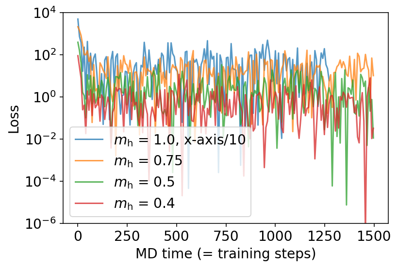
Figure 6: Loss history in prior run of HMC. Horizontal axis coincides with the training steps. (Left) Summary plot for $m_{\text{h}}=1.0,0.75,0.5,0.4$ in the log scale. (Right) Loss history for $m_{\text{h}}=0.4$ in the linear scale. The inside plot is the same one except for the range of the horizontal axis.

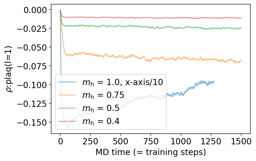
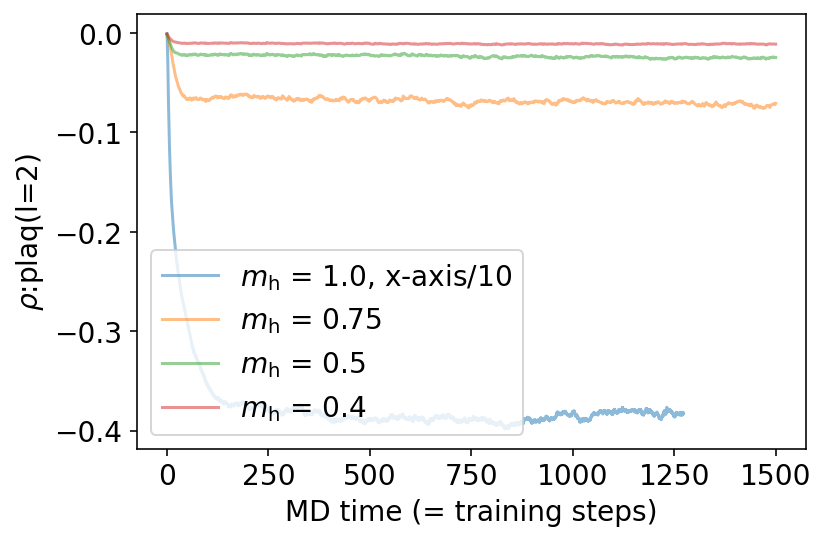
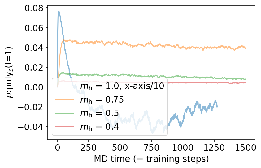
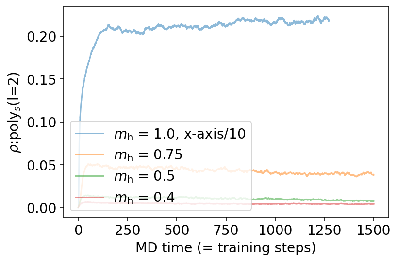
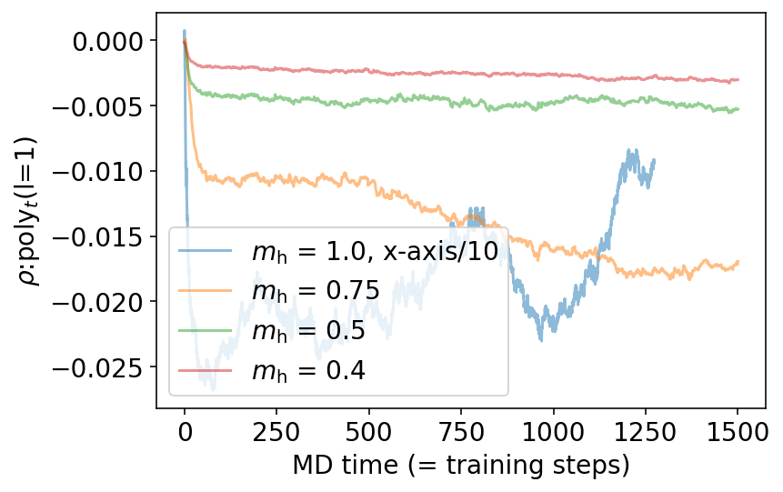
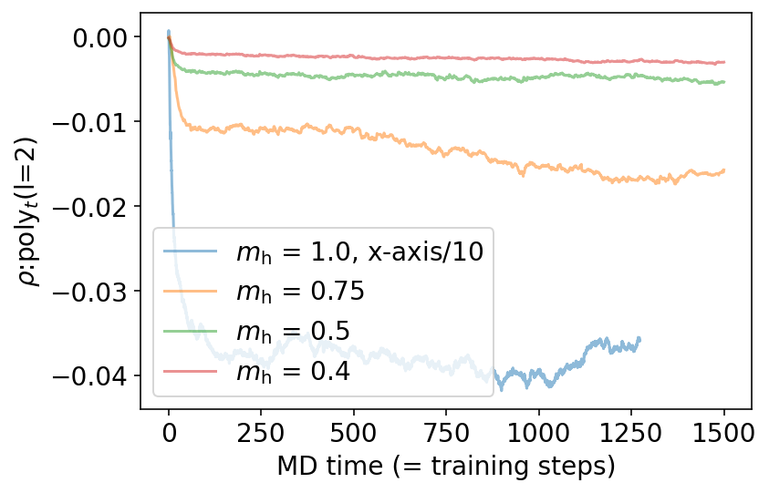
Figure 7: Training history of weights in the neural network. From top to bottom, coefficients of plaquette, Polyakov loop for spatial directions, and Polyakov loop for temporal directions are displayed. Left panels and right panels are weights in the first layer and the second layer.

References

- Akinori Tanaka [2021] K. H. Akinori Tanaka, Akio Tomiya, Deep Learning and Physics (Springer, Switzerland, 2021).
- Bronstein et al. [2021] M. M. Bronstein, J. Bruna, T. Cohen, and P. Veličković, Geometric deep learning: Grids, groups, graphs, geodesics, and gauges (2021), arXiv:2104.13478 [cs.LG] .
- Morningstar and Peardon [2004] C. Morningstar and M. Peardon, Analytic smearing ofsu(3)link variables in lattice qcd, Physical Review D 69, 10.1103/physrevd.69.054501 (2004).
- Ding et al. [2015] H.-T. Ding, F. Karsch, and S. Mukherjee, Thermodynamics of strong-interaction matter from Lattice QCD, Int. J. Mod. Phys. E 24, 1530007 (2015), arXiv:1504.05274 [hep-lat] .
- Miura [2019] K. Miura, Review of Lattice QCD Studies of Hadronic Vacuum Polarization Contribution to Muon g-2, PoS LATTICE2018, 010 (2019), arXiv:1901.09052 [hep-lat] .
- Aoki et al. [2020] S. Aoki et al. (Flavour Lattice Averaging Group), FLAG Review 2019: Flavour Lattice Averaging Group (FLAG), Eur. Phys. J. C 80, 113 (2020), arXiv:1902.08191 [hep-lat] .
- Albanese et al. [1987] M. Albanese et al. (APE), Glueball Masses and String Tension in Lattice QCD, Phys. Lett. B 192, 163 (1987).
- Kamleh et al. [2004] W. Kamleh, D. B. Leinweber, and A. G. Williams, Hybrid Monte Carlo with fat link fermion actions, Phys. Rev. D 70, 014502 (2004), arXiv:hep-lat/0403019 .
- Hasenfratz et al. [2007] A. Hasenfratz, R. Hoffmann, and S. Schaefer, Hypercubic smeared links for dynamical fermions, Journal of High Energy Physics 2007, 029–029 (2007).
- Blum et al. [1997] T. Blum, C. E. Detar, S. A. Gottlieb, K. Rummukainen, U. M. Heller, J. E. Hetrick, D. Toussaint, R. L. Sugar, and M. Wingate, Improving flavor symmetry in the Kogut-Susskind hadron spectrum, Phys. Rev. D 55, R1133 (1997), arXiv:hep-lat/9609036 .
- Orginos et al. [1999] K. Orginos, D. Toussaint, and R. L. Sugar (MILC), Variants of fattening and flavor symmetry restoration, Phys. Rev. D 60, 054503 (1999), arXiv:hep-lat/9903032 .
- Follana et al. [2007] E. Follana, Q. Mason, C. Davies, K. Hornbostel, G. P. Lepage, J. Shigemitsu, H. Trottier, and K. Wong, Highly improved staggered quarks on the lattice with applications to charm physics, Physical Review D 75, 10.1103/physrevd.75.054502 (2007).
- Bazavov et al. [2010] A. Bazavov, C. Bernard, C. DeTar, W. Freeman, S. Gottlieb, U. M. Heller, J. E. Hetrick, J. Laiho, L. Levkova, M. Oktay, and et al., Scaling studies of qcd with the dynamical highly improved staggered quark action, Physical Review D 82, 10.1103/physrevd.82.074501 (2010).
- Luscher [2013] M. Luscher, Chiral symmetry and the Yang–Mills gradient flow, JHEP 04, 123, arXiv:1302.5246 [hep-lat] .
- Tanaka and Tomiya [2017] A. Tanaka and A. Tomiya, Towards reduction of autocorrelation in HMC by machine learning, (2017), arXiv:1712.03893 [hep-lat] .
- Zhou et al. [2019] K. Zhou, G. Endrődi, L.-G. Pang, and H. Stöcker, Regressive and generative neural networks for scalar field theory, Phys. Rev. D 100, 011501 (2019), arXiv:1810.12879 [hep-lat] .
- Pawlowski and Urban [2020] J. M. Pawlowski and J. M. Urban, Reducing Autocorrelation Times in Lattice Simulations with Generative Adversarial Networks, Mach. Learn. Sci. Tech. 1, 045011 (2020), arXiv:1811.03533 [hep-lat] .
- Albergo et al. [2019] M. S. Albergo, G. Kanwar, and P. E. Shanahan, Flow-based generative models for Markov chain Monte Carlo in lattice field theory, Phys. Rev. D 100, 034515 (2019), arXiv:1904.12072 [hep-lat] .
- Rezende et al. [2020] D. J. Rezende, G. Papamakarios, S. Racanière, M. S. Albergo, G. Kanwar, P. E. Shanahan, and K. Cranmer, Normalizing flows on tori and spheres (2020), arXiv:2002.02428 [stat.ML] .
- Kanwar et al. [2020] G. Kanwar, M. S. Albergo, D. Boyda, K. Cranmer, D. C. Hackett, S. Racanière, D. J. Rezende, and P. E. Shanahan, Equivariant flow-based sampling for lattice gauge theory, Phys. Rev. Lett. 125, 121601 (2020), arXiv:2003.06413 [hep-lat] .
- Boyda et al. [2020] D. Boyda, G. Kanwar, S. Racanière, D. J. Rezende, M. S. Albergo, K. Cranmer, D. C. Hackett, and P. E. Shanahan, Sampling using gauge equivariant flows, (2020), arXiv:2008.05456 [hep-lat] .
- Albergo et al. [2021] M. S. Albergo, D. Boyda, D. C. Hackett, G. Kanwar, K. Cranmer, S. Racanière, D. J. Rezende, and P. E. Shanahan, Introduction to Normalizing Flows for Lattice Field Theory, (2021), arXiv:2101.08176 [hep-lat] .
- Favoni et al. [2020] M. Favoni, A. Ipp, D. I. Müller, and D. Schuh, Lattice gauge equivariant convolutional neural networks, (2020), arXiv:2012.12901 [hep-lat] .
- Nagai et al. [2020a] Y. Nagai, M. Okumura, K. Kobayashi, and M. Shiga, Self-learning hybrid monte carlo: A first-principles approach, Physical Review B 102, 10.1103/physrevb.102.041124 (2020a).
- He et al. [2015] K. He, X. Zhang, S. Ren, and J. Sun, Deep residual learning for image recognition (2015), arXiv:1512.03385 [cs.CV] .
- He et al. [2016] K. He, X. Zhang, S. Ren, and J. Sun, Identity mappings in deep residual networks (2016), arXiv:1603.05027 [cs.CV] .
- Chen et al. [2019] R. T. Q. Chen, Y. Rubanova, J. Bettencourt, and D. Duvenaud, Neural ordinary differential equations (2019), arXiv:1806.07366 [cs.LG] .
- Lüscher [2009] M. Lüscher, Trivializing maps, the wilson flow and the hmc algorithm, Communications in Mathematical Physics 293, 899–919 (2009).
- Note [1] Conventional neural networks and their training are explain in appendix in details.
- Capitani et al. [2006] S. Capitani, S. Durr, and C. Hoelbling, Rationale for UV-filtered clover fermions, JHEP 11, 028, arXiv:hep-lat/0607006 .
- Behler and Parrinello [2007] J. Behler and M. Parrinello, Generalized neural-network representation of high-dimensional potential-energy surfaces, Phys. Rev. Lett. 98, 146401 (2007).
- Nagai et al. [2020b] Y. Nagai, M. Okumura, and A. Tanaka, Self-learning monte carlo method with behler-parrinello neural networks, Physical Review B 101, 10.1103/physrevb.101.115111 (2020b).
- Lüscher [2010] M. Lüscher, Properties and uses of the Wilson flow in lattice QCD, JHEP 08, 071, [Erratum: JHEP 03, 092 (2014)], arXiv:1006.4518 [hep-lat] .
- Fukaya et al. [2014] H. Fukaya, S. Aoki, G. Cossu, S. Hashimoto, T. Kaneko, and J. Noaki (JLQCD), Overlap/Domain-wall reweighting, PoS LATTICE2013, 127 (2014), arXiv:1311.4646 [hep-lat] .
- Tomiya et al. [2017] A. Tomiya, G. Cossu, S. Aoki, H. Fukaya, S. Hashimoto, T. Kaneko, and J. Noaki, Evidence of effective axial U(1) symmetry restoration at high temperature QCD, Phys. Rev. D 96, 034509 (2017), [Addendum: Phys.Rev.D 96, 079902 (2017)], arXiv:1612.01908 [hep-lat] .
- Nagai et al. [2020c] Y. Nagai, A. Tanaka, and A. Tomiya, Self-learning Monte-Carlo for non-abelian gauge theory with dynamical fermions, (2020c), arXiv:2010.11900 [hep-lat] .
- Matsumoto et al. [2021] T. Matsumoto, M. Kitazawa, and Y. Kohno, Classifying topological charge in SU(3) Yang–Mills theory with machine learning, PTEP 2021, 023D01 (2021), arXiv:1909.06238 [hep-lat] .

References

- [1] Koji Hashimoto Akinori Tanaka, Akio Tomiya. Deep Learning and Physics. Springer, Switzerland, 2021.
- [2] Michael M. Bronstein, Joan Bruna, Taco Cohen, and Petar Veličković. Geometric deep learning: Grids, groups, graphs, geodesics, and gauges, 2021.
- [3] Colin Morningstar and Mike Peardon. Analytic smearing of su(3)link variables in lattice qcd. Physical Review D, 69(5), Mar 2004.
- [4] Heng-Tong Ding, Frithjof Karsch, and Swagato Mukherjee. Thermodynamics of strong-interaction matter from Lattice QCD. Int. J. Mod. Phys. E, 24(10):1530007, 2015.
- [5] Kohtaroh Miura. Review of Lattice QCD Studies of Hadronic Vacuum Polarization Contribution to Muon g-2. PoS, LATTICE2018:010, 2019.
- [6] S. Aoki et al. FLAG Review 2019: Flavour Lattice Averaging Group (FLAG). Eur. Phys. J. C, 80(2):113, 2020.
- [7] M. Albanese et al. Glueball Masses and String Tension in Lattice QCD. Phys. Lett. B, 192:163–169, 1987.
- [8] Waseem Kamleh, Derek B. Leinweber, and Anthony G. Williams. Hybrid Monte Carlo with fat link fermion actions. Phys. Rev. D, 70:014502, 2004.
- [9] Anna Hasenfratz, Roland Hoffmann, and Stefan Schaefer. Hypercubic smeared links for dynamical fermions. Journal of High Energy Physics, 2007(05):029–029, May 2007.
- [10] Tom Blum, Carleton E. Detar, Steven A. Gottlieb, Kari Rummukainen, Urs M. Heller, James E. Hetrick, Doug Toussaint, R. L. Sugar, and Matthew Wingate. Improving flavor symmetry in the Kogut-Susskind hadron spectrum. Phys. Rev. D, 55:R1133–R1137, 1997.
- [11] Kostas Orginos, Doug Toussaint, and R. L. Sugar. Variants of fattening and flavor symmetry restoration. Phys. Rev. D, 60:054503, 1999.
- [12] E. Follana, Q. Mason, C. Davies, K. Hornbostel, G. P. Lepage, J. Shigemitsu, H. Trottier, and K. Wong. Highly improved staggered quarks on the lattice with applications to charm physics. Physical Review D, 75(5), Mar 2007.
- [13] A. Bazavov, C. Bernard, C. DeTar, W. Freeman, Steven Gottlieb, U. M. Heller, J. E. Hetrick, J. Laiho, L. Levkova, M. Oktay, and et al. Scaling studies of qcd with the dynamical highly improved staggered quark action. Physical Review D, 82(7), Oct 2010.
- [14] Martin Luscher. Chiral symmetry and the Yang–Mills gradient flow. JHEP, 04:123, 2013.
- [15] Akinori Tanaka and Akio Tomiya. Towards reduction of autocorrelation in HMC by machine learning. 12 2017.
- [16] Kai Zhou, Gergely Endrődi, Long-Gang Pang, and Horst Stöcker. Regressive and generative neural networks for scalar field theory. Phys. Rev. D, 100(1):011501, 2019.
- [17] Jan M. Pawlowski and Julian M. Urban. Reducing Autocorrelation Times in Lattice Simulations with Generative Adversarial Networks. Mach. Learn. Sci. Tech., 1:045011, 2020.
- [18] M. S. Albergo, G. Kanwar, and P. E. Shanahan. Flow-based generative models for Markov chain Monte Carlo in lattice field theory. Phys. Rev. D, 100(3):034515, 2019.
- [19] Danilo Jimenez Rezende, George Papamakarios, Sébastien Racanière, Michael S. Albergo, Gurtej Kanwar, Phiala E. Shanahan, and Kyle Cranmer. Normalizing flows on tori and spheres, 2020.
- [20] Gurtej Kanwar, Michael S. Albergo, Denis Boyda, Kyle Cranmer, Daniel C. Hackett, Sébastien Racanière, Danilo Jimenez Rezende, and Phiala E. Shanahan. Equivariant flow-based sampling for lattice gauge theory. Phys. Rev. Lett., 125(12):121601, 2020.
- [21] Denis Boyda, Gurtej Kanwar, Sébastien Racanière, Danilo Jimenez Rezende, Michael S. Albergo, Kyle Cranmer, Daniel C. Hackett, and Phiala E. Shanahan. Sampling using gauge equivariant flows. 8 2020.
- [22] Michael S. Albergo, Denis Boyda, Daniel C. Hackett, Gurtej Kanwar, Kyle Cranmer, Sébastien Racanière, Danilo Jimenez Rezende, and Phiala E. Shanahan. Introduction to Normalizing Flows for Lattice Field Theory. 1 2021.
- [23] Matteo Favoni, Andreas Ipp, David I. Müller, and Daniel Schuh. Lattice gauge equivariant convolutional neural networks. 12 2020.
- [24] Yuki Nagai, Masahiko Okumura, Keita Kobayashi, and Motoyuki Shiga. Self-learning hybrid monte carlo: A first-principles approach. Physical Review B, 102(4), Jul 2020.
- [25] Kaiming He, Xiangyu Zhang, Shaoqing Ren, and Jian Sun. Deep residual learning for image recognition, 2015.
- [26] Kaiming He, Xiangyu Zhang, Shaoqing Ren, and Jian Sun. Identity mappings in deep residual networks, 2016.
- [27] Ricky T. Q. Chen, Yulia Rubanova, Jesse Bettencourt, and David Duvenaud. Neural ordinary differential equations, 2019.
- [28] Martin Lüscher. Trivializing maps, the wilson flow and the hmc algorithm. Communications in Mathematical Physics, 293(3):899–919, Nov 2009.
- [29] Stefano Capitani, Stephan Durr, and Christian Hoelbling. Rationale for UV-filtered clover fermions. JHEP, 11:028, 2006.
- [30] Jörg Behler and Michele Parrinello. Generalized neural-network representation of high-dimensional potential-energy surfaces. Phys. Rev. Lett., 98:146401, Apr 2007.
- [31] Yuki Nagai, Masahiko Okumura, and Akinori Tanaka. Self-learning monte carlo method with behler-parrinello neural networks. Physical Review B, 101(11), Mar 2020.
- [32] Martin Lüscher. Properties and uses of the Wilson flow in lattice QCD. JHEP, 08:071, 2010. [Erratum: JHEP 03, 092 (2014)].
- [33] H. Fukaya, S. Aoki, G. Cossu, S. Hashimoto, T. Kaneko, and J. Noaki. Overlap/Domain-wall reweighting. PoS, LATTICE2013:127, 2014.
- [34] A. Tomiya, G. Cossu, S. Aoki, H. Fukaya, S. Hashimoto, T. Kaneko, and J. Noaki. Evidence of effective axial U(1) symmetry restoration at high temperature QCD. Phys. Rev. D, 96(3):034509, 2017. [Addendum: Phys.Rev.D 96, 079902 (2017)].
- [35] Yuki Nagai, Akinori Tanaka, and Akio Tomiya. Self-learning Monte-Carlo for non-abelian gauge theory with dynamical fermions. 10 2020.
- [36] Takuya Matsumoto, Masakiyo Kitazawa, and Yasuhiro Kohno. Classifying topological charge in SU(3) Yang–Mills theory with machine learning. PTEP, 2021(2):023D01, 2021.
- [37] Ding-Xuan Zhou. Universality of deep convolutional neural networks, 2018.
- [38] Patrick Kidger and Terry Lyons. Universal approximation with deep narrow networks, 2020.
- [39] Paulo Tabuada and Bahman Gharesifard. Universal approximation power of deep residual neural networks via nonlinear control theory, 2020.
- [40] Jesse Johnson. Deep, skinny neural networks are not universal approximators, 2018.
- [41] S. Duane, A. D. Kennedy, B. J. Pendleton, and D. Roweth. Hybrid Monte Carlo. Phys. Lett. B, 195:216–222, 1987.
- [42] M. A. Clark. The Rational Hybrid Monte Carlo Algorithm. PoS, LAT2006:004, 2006.
- [43] George Cybenko. Approximation by superpositions of a sigmoidal function. Mathematics of control, signals and systems, 2(4):303–314, 1989.
- [44] Yuki Nagai and Akio Tomiya. Latticeqcd.jl. Paper is in preparation, https://github.com/akio-tomiya/LatticeQCD.jl.
- [45] Jeff Bezanson, Alan Edelman, Stefan Karpinski, and Viral B. Shah. Julia: A fresh approach to numerical computing, 2015.