Muon reconstruction with a convolutional neural network in the JUNO detector

Abstract

The Jiangmen Underground Neutrino Observatory (JUNO) is designed to determine the neutrino mass ordering and measure neutrino oscillation parameters. A precise muon reconstruction is crucial to reduce one of the major backgrounds induced by cosmic muons. This article proposes a novel muon reconstruction method based on convolutional neural network (CNN) models. In this method, the track information reconstructed by the top tracker is used for network training. The training dataset is augmented by applying a rotation to muon tracks to compensate for the limited angular coverage of the top tracker. The muon reconstruction with the CNN model can produce unbiased tracks with performance that spatial resolution is better than 10 cm and angular resolution is better than 0.6 degrees. By using a GPU accelerated implementation a speedup factor of 100 compared to existing CPU techniques has been demonstrated.

Introduction

Jiangmen Underground Neutrino Observatory (JUNO) Djurcic:2015vqa is a liquid scintillator detector that is designed to determine the neutrino mass ordering and to precisely measure neutrino oscillation parameters. Its location 53 km away from both Yangjiang and Taishan nuclear power plants in Southern China is chosen to optimize the oscillation measurement sensitivity. A schematic view of the JUNO detector is shown in Fig. 1. The innermost central detector (CD) is 20 kiloton of liquid scintillator contained by an acrylic sphere and instrumented with $\sim$18,000 20-inch and 25,600 3-inch photomultipliers tubes (PMTs). The CD is submerged in a water pool which is instrumented with a further 2,400 PMTs forming the Water Cerenkov Detector (WCD). The Top Tracker (TT), located above the CD and WCD, is a 3-layer muon tracker detector with size 47 m $\times$ 20 m $\times$ 3 m providing precise atmospheric muon tracking over about 60% of the water pool. Ionizing particles cause excitations within the scintillator which subsequently de-exite resulting in the emission of scintillation photons. These photons propagate through the detector undergoing scattering, absorption and re-emission as well as refraction and reflection at material boundaries before some reach the PMTs. The charge and time information measured by the PMTs enables the originating vertex position and energy to be reconstructed.

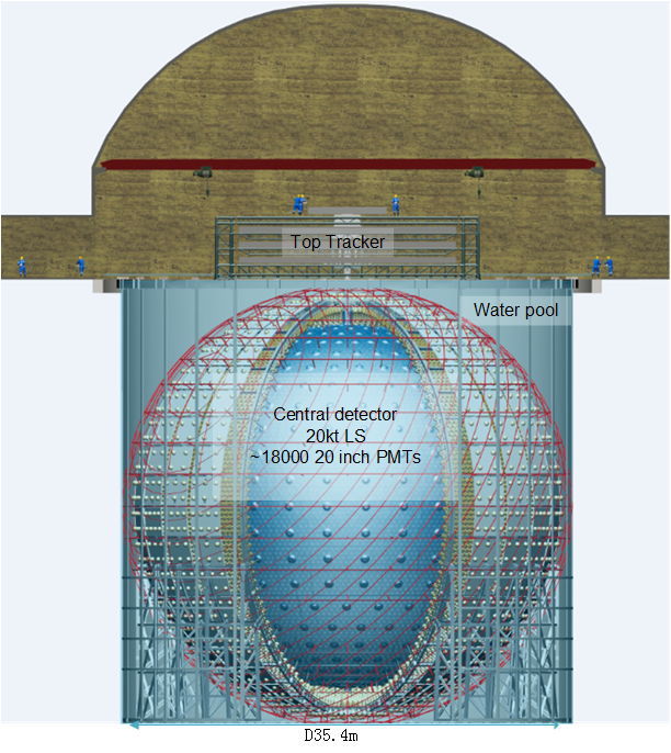
Figure 1: A schematic view of the JUNO detector.

The primary background for neutrino detection arises from ⁹Li/ ⁸He induced by muon spallation in the liquid scintillator or muon shower particles. This background can be reduced by excluding a veto volume along the muon track within a time window surrounding the time at which the muon passes through the detector. A precise muon reconstruction directly allows the veto volume and time windows to be reduced which increases the livetime achievable by the JUNO detector.

The vital importance of muon reconstruction for JUNO has led to the development of several muon reconstruction methods including:

• Muon reconstruction with a geometrical model Genster:2018caz which is based on the geometrical shape of the first light and provides a spatial resolution of 20 cm and an angular resolution of 1.6 degree over the whole detector.

• Muon tracking with the fastest light Zhang:2018kag which uses the least squares fit to the PMT first hit time (FHT) measurements. After correction of the FHT for each PMT, the reconstruction yields spatial resolution less than 3 cm and angular resolution of less than 0.4 degree.

This article reports a novel alternative technique for muon reconstruction that applies deep learning techniques and benefits from GPU acceleration. This technique has the advantages of speed and avoids the need to develop detailed optical models or to interpret calibration data. All studies have been based on JUNO Monte Carlo simulation data.

Treating the readout of the whole detector as an image composed of pixel values from PMT charge and time measurements allows image classification techniques to be applied to track finding and fitting. For image processing tasks, Convolutional Neural Networks (CNN) have been widely used in many areas such as image classification Russakovsky:2014lic , object detection girshick2014rich and image segmentation long2015fully . Within high energy physics, image processing with CNN has been used in jet classification Kasieczka:2017nvn ; Baldi:2016fql and event classification Bhimji:2017qvb ; Aurisano:2016jvx . In this paper, the CNN is adopted to perform muon track reconstruction in the CD detector.

This paper is organized into a description of how the training and testing datasets were prepared in section 2 followed by an explanation of the chosen deep neural network architecture and training procedure in section 3. Performance metrics of the muon reconstruction are presented in section 4 and a discussion of possible challenges for the application of this technique to experimental data are given in section 5, followed by the conclusions of this study summarized in section 6.

Dataset and muon reconstruction model

Simulation of single muon tracks

In this study all Monte Carlo (MC) simulated muon events used for network training and testing are produced by the official JUNO simulation framework Huang:2017dkh ; Lin:2017usg which is based on the Geant4 toolkit allison2016recent . The underground muon sample before input into detector are generated by the muon transportation software MUSIC Kudryavtsev:2008qh with JUNO mountain profile and the parameterized Gaisser formula of muon Guan:2015vja at the mountain surface. The energy range of cosmic muon reaching the JUNO detector is from 0.1 GeV to 10 TeV in simulation and the average energy is about 207 GeV. The flux is about 4 $\times$ 10^-3 Hz / m². There are about 90$\%$ muons with single track and about 10$\%$ muons with multiple tracks in the muon events. Only the events with 200 GeV muon track are selected for this study, so that the muons will go through the whole detector and exit at the bottom.

Along the muon trajectory through the materials of the detector geometry the Geant4 toolkit simulates physics processes including ionization and nuclear interactions. Muons passing through the scintillator result in excitations of the molecules of the scintillating medium which subsequently de-excite producing photons. In addition as muons travel through both the water pool and the scintillator their charged nature results in the generation of photons from Cerenkov radiation. Both scintillation photons and Cerenkov photons are propagated through the detector taking into account optical processes such as scattering, absorption and re-emission. A fraction of the propagated photons reach PMTs and eject a photo-electron from the photocathode resulting in electronic signals for the charge and arrival time. PMT characteristics including the quantum efficiency and collection efficiency are measured and used as inputs to the simulation.

Figure 2 illustrates a muon track passing through the liquid scintillator (LS), together with the positions of PMTs that detect optical photons emitted along the muon trajectory.

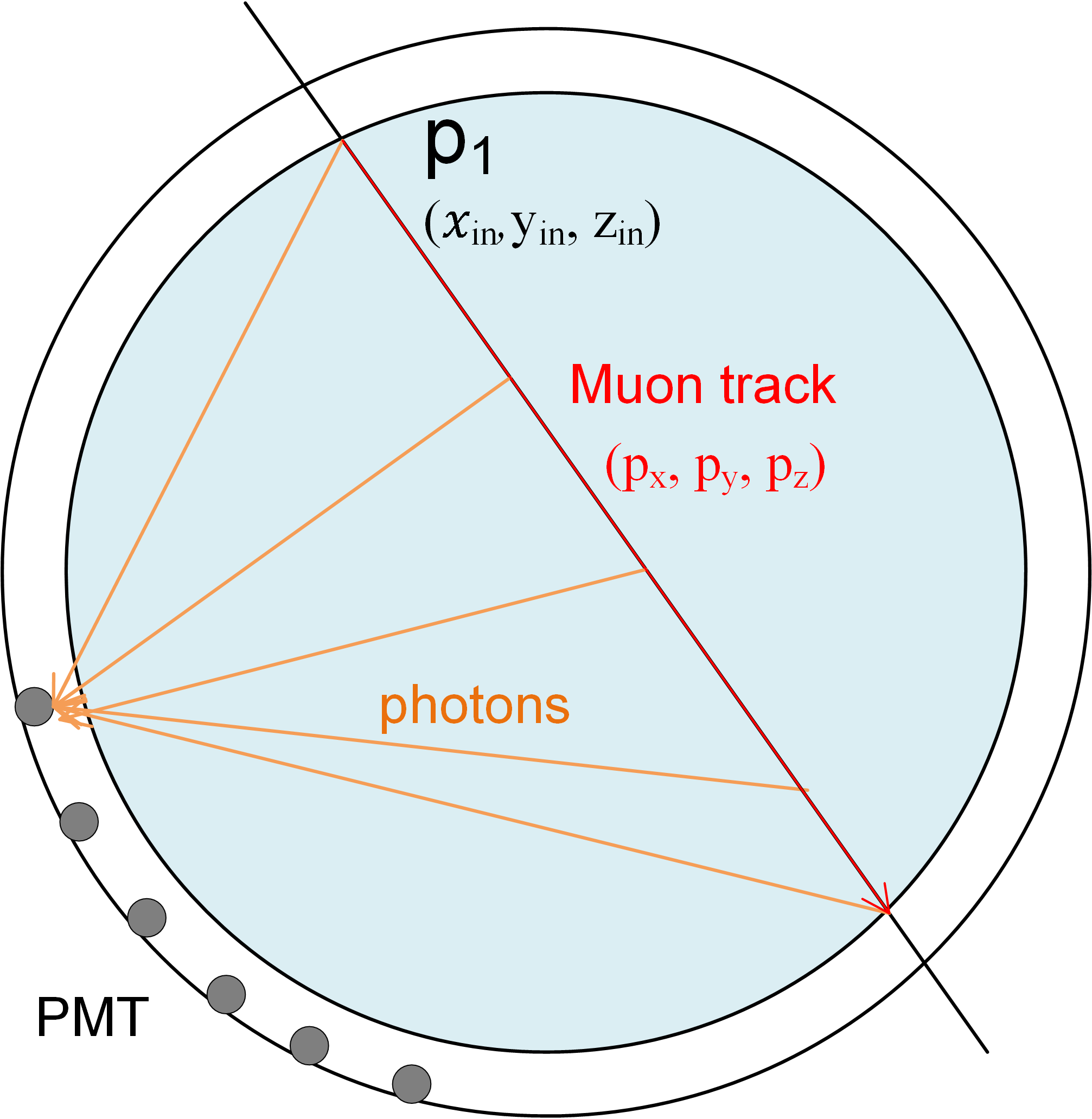
Figure 2: Schematic of muon track, optical photon paths and PMT positions. The shaded area represents the LS.

Comparisons of simulated and real experimental data often reveal some differences. This presents a problem as neural networks trained with simulated samples may learn features that differ from those present in the real data causing the model to be invalid. As real JUNO experimental data is not yet available a comparison between independent aspects of the simulated data is used as a cross check. The muon track parameters obtained from the top tracker (TT) reconstruction Djurcic:2015vqa are used as an independent alternative for training the neural network and compared with results obtained by training based on the MC truth information.

Modeling of muon reconstruction

Muon reconstruction uses the first light arrival times and number of photoelectrons detected by all the PMTs as well as the positions of the PMTs. The muon track is modeled using its direction vector ($p_{x},p_{y},p_{z}$) and the intersection position of the track with surface of the LS sphere $\vec{r}_{\scriptsize\textrm{in}}$ = ($x_{\scriptsize\textrm{in}},y_{\scriptsize\textrm{in}},z_{\scriptsize\textrm{in}}$) using a coordinate system which origin at the center of the LS sphere.

$$\vec{track}=(x_{\scriptsize\textrm{in}},y_{\scriptsize\textrm{in}},z_{\scriptsize\textrm{in}},p_{x},p_{y},p_{z}).$$ (1)

Muon reconstruction is the estimation of the 6 independent track parameters $\vec{track}^{\scriptsize\textrm{rec}}$ from PMT measurements of the numbers of photoelectrons ($\vec{Q}$), fastest light arrival times ($\vec{T}$) as well as the positions of all the PMTs ($\vec{R}$).

$$\vec{track}^{\scriptsize\textrm{rec}}=f(\vec{Q},\vec{T},\vec{R}).$$ (2)

Reconstruction performance is assessed using the angle $\alpha$ between the true track and the reconstructed track and the difference between the distance to CD center $\Delta$D between the true and reconstructed track.

Muon tracking and selection with Top-Tracker

Comparisons of TT reconstructed muon tracks with MC truth tracks show that it is necessary to apply track quality criteria to select well reconstructed muons. Table 1 shows the reconstruction performance for a series of selection criteria on the number of the hit TT layers ($N_{\scriptsize\textrm{point}}$), the least squares value of TT reconstruction ($\chi^{2}$) and the number of activated scintillator bars in the X, Y direction of the layer ($N_{\scriptsize\textrm{channel}}$).

The reconstruction performance is substantially improved within the high quality selection. Further quality criteria tested did not provide significant performance gains. The highest quality selection 4 was used for the network training with TT tracks.

Table 1: TT reconstruction performance for a sequence of selection criteria.

Selection	1	2	3	4
Events	145K	130K	46K	40K
$N_{\scriptsize\textrm{point}}$ Cuts	-	$>$2	$>$2	$>$2
$\chi^{2}$ Cuts	-	-	$<$0.2	$<$0.2
$N_{\scriptsize\textrm{channel}}$ Cuts	-	-	-	$<$8
$\alpha$ Mean / degree	0.30	0.23	0.21	0.20
$\alpha$ RMS / degree	1.28	0.58	0.30	0.16
$\Delta$D Mean / mm	1.1	0.8	0.6	0.3
$\Delta$D RMS / mm	321	157	91	75

Rotation method based data augmentation

As the TT partially covers the water pool it is only able to reconstruct muons over a limited solid angle region. Figure 3 shows the distributions of CD sphere injection points for reconstructed TT muons in the upper plot and for the the MC truth tracks in the lower plot. A rotation method has been developed that effectively extends the angular range of the training sample using a rotational symmetry assumption.

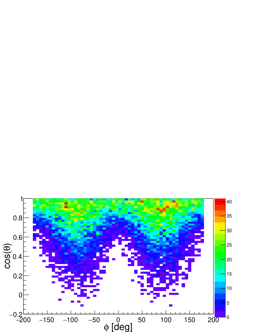
(a) Injection points distribution of TT reconstruction

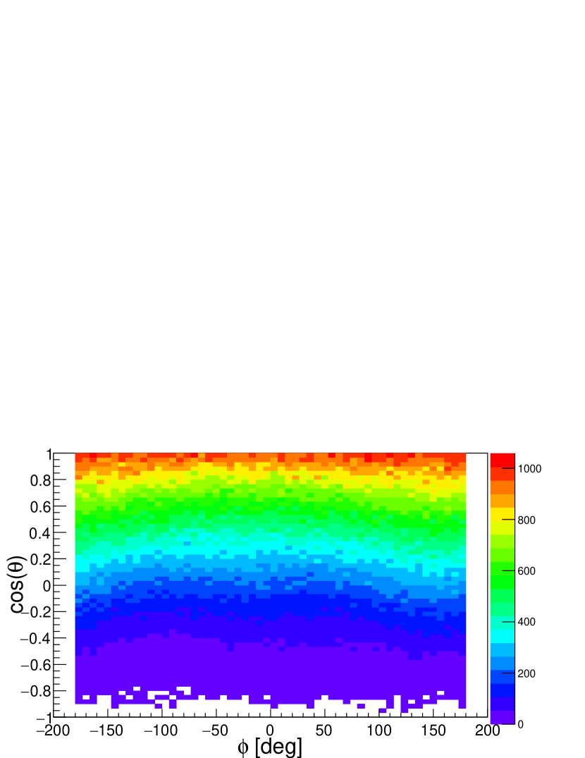
(b) Injection points distribution of MC truth tracks

Figure 3: The two dimension distribution of ($\cos\theta$, $\phi$), where ($\theta$, $\phi$) are the injection positions at the surface of the LS sphere in spherical coordinates. The injection positions are at the north pole of LS sphere when cos($\theta$) = 1 ($\theta$ = 0 deg). The distribution modulated with and without TT geometry and reconstruction is shown in (a) and (b) respectively. In Fig (a), the non-uniform distribution along $\phi$ is influenced by the TT geometry. In Fig (b), the distribution is not uniform along $\phi$, because the underground muon distribution was modulated by the mountain profile above.

The rotation method is illustrated in Fig. 4 showing how an event is rotated and a new event is generated based on the reconstructed tracks. A randomized rotation matrix of each event is defined considering a new injection point and rotation angle $\omega$ of the track around the vector $\vec{v}$. The track and the positions of PMTs are rotated together using the same rotation matrix. After the randomized rotation, a rejection sampling is applied to get a new position that conforms to the expectation of the distribution.

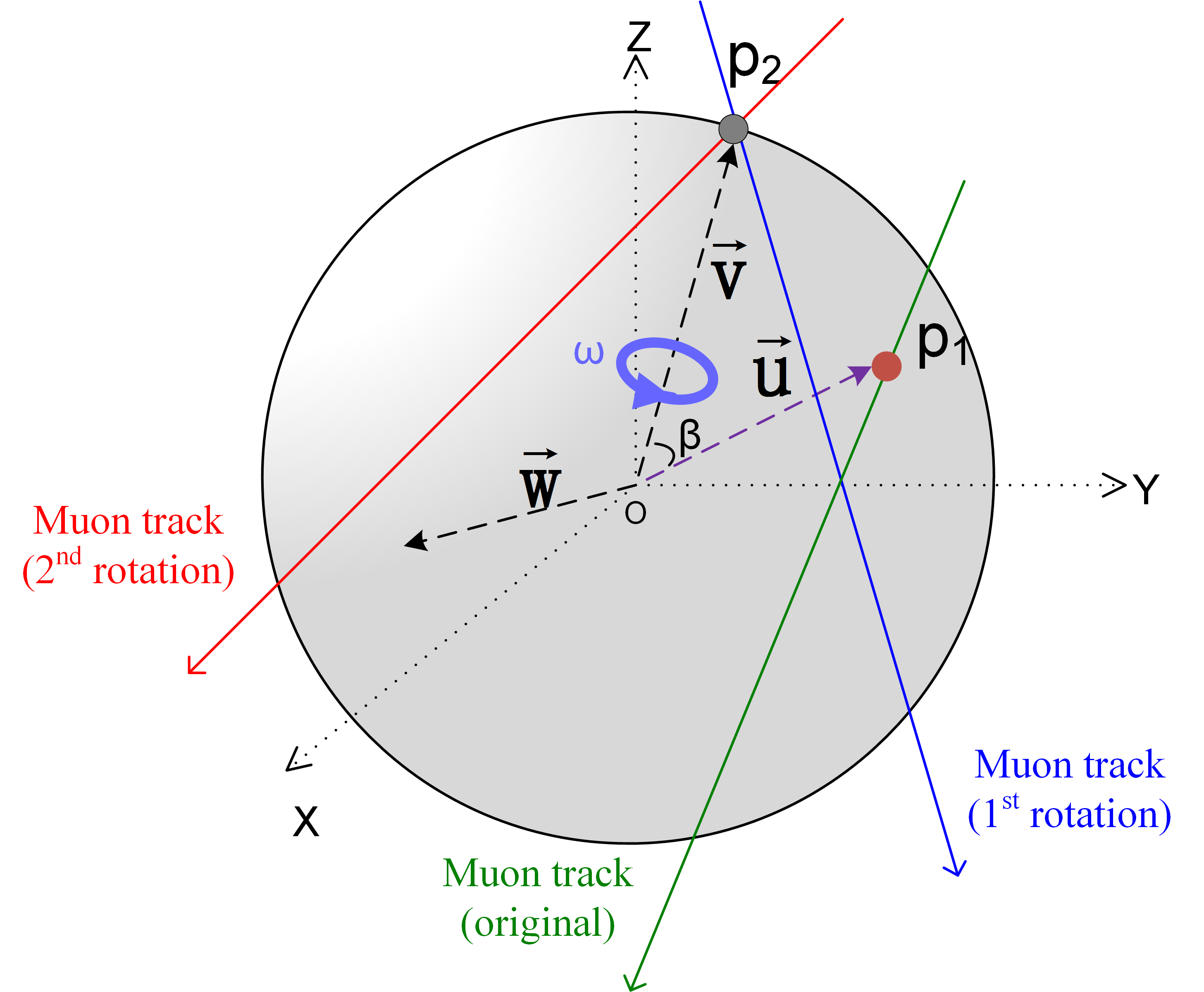
Figure 4: Schematic diagram of the rotation method. The original muon is shown in green. First the track is rotated along the $\vec{w}$ with angle $\beta$, where $\vec{w}=\vec{u}\times\vec{v}$. After the first rotation, the track in blue is then rotated around $\vec{v}$ with angle $\omega$. The final track is shown in red. The detector is also rotated using the same rotation matrix.

For muon events reconstructed by TT, after using the rotation method, the distribution of the injection point is shown in Fig. 5. Comparing the Fig. 3 (b) and Fig. 5, it can be found that the injection point distribution after rotation is similar to the one from cosmic muon in CD which basically extends the ranges of injection points.

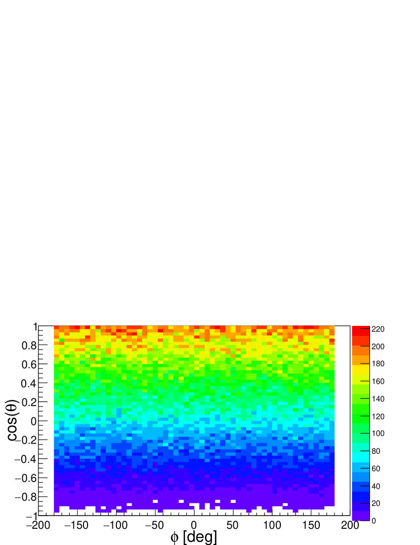
Figure 5: Injection point distribution after rotation

Dataset Composition

Application of CNN models to muon reconstruction requires the fixed PMT positions and measurements of PMT charge and times to be converted into image arrays. All PMT positions (x,y,z) are converted into two-dimensional spherical coordinates ($\theta$,$\phi$) using the equidistant cylindrical projection.

Example images of the charge Q and time T channels at the PMT pixel positions are shown in the Fig. 6. The charge channel has two clusters corresponding to the muon entry and exit points at the CD sphere surface and the time T channel has a valley of low values in the region of the muon entry point. These two channels are combined together in an image pixel array, with each pixel having two channel values with the values of charge Q and time T, while the values for pixels that do not correspond to PMTs are set to zero. Then the feature standardization pal2016preprocessing is applied to each channel of the image pixel array for the normalization of the image before entering the neural network:

$$X^{\prime}=(X-\mu)/\sigma$$ (3)

where $X$ is the original data, $X^{\prime}$ is the normalized data, $\mu$ is the mean of $X$ and $\sigma$ is the standard deviation of $X$.

In the training, the label of the direction vector ($p_{x},p_{y},p_{z}$) and intersection position vector ($x_{\scriptsize\textrm{in}},y_{\scriptsize\textrm{in}},z_{\scriptsize\textrm{in}}$) have been normalized to unit vectors, respectively.

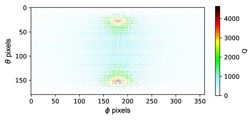
(a) Image of channel Q

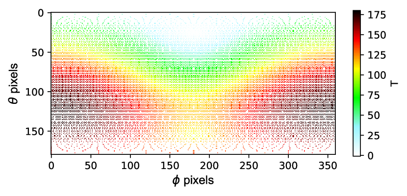
(b) Image of channel T

Figure 6: Charge and time channel images for a vertical downwards muon track with entry point at spherical coordinates (25,180) degrees on the CD sphere. The color scale from blue through to red represents increasing values.

The training and testing samples used in this study are shown in Table 2. The sample of directly simulated muons is split into training, validation and testing samples named “Training MC”, “Validation MC” and “Testing MC” in the table. The training data set obtained by TT reconstruction and rotation is called “training TT$\_$rot”.

Table 2: Dataset

Dataset	Events	Image size	Label
Training MC	300K	180x360 QT	MC truth
Training TT$\_$rot	300K	180x360 QT	TT reconstruction
Validation MC	20K	180x360 QT	MC truth
Testing MC	20K	180x360 QT	MC truth

Network architecture

The use of artificial neural networks to solve complex problems has been explored since the 1940s. In recent years, with the dramatic increase in available computing power, it has become feasible to use computationally intensive neural networks with many inner layers. These neural networks with many computational layers are called deep neural networks (DNN), which can learn various potential features in large amounts of data. Convolutional neural network (CNN or ConvNet) are one form of deep neural network. CNN consist of one or more convolutional layers and a top fully connected layer, as well as associated weights and pooling layers. This structure makes convolutional neural networks suitable for processing two-dimensional image data and extracting features from the data efficiently.

Model architecture

The network model architecture adopted in this study and illustrated in Fig. 7 is based on the VGGNet16 simonyan2014very configuration. It is composed of an input layer, convolutional layers, activation layers, pooling layers and fully connected layers. The input layer is the 2-channel (Q and T) image converted from the muon event data.

The principal elements in this model are blocks of three convolution layers with a 3$\times$3 convolutional kernel followed by a pooling layer (max pooling) scherer2010evaluation . The convolutional layers are used to perform data feature extraction. The max pooling layer is used for signal downsampling, reducing the data size input to the next layer and also reducing the impact of local data on the result which makes the results more robust. As shown in the study simonyan2014very the use of three 3$\times$3 convolutional layers has several advantages. Firstly this architecture has the same large effective receptive field as a 7$\times$7 convolutional layer, but decreases the number of learning parameters by almost a factor of two. Secondly, it can inject more non-linearity operations between the two convolution layers which enhanced the ability to learn features.

The fully connected hidden layers convert the abstract feature signal into the output of the prediction task. After some tries, the number of neurons at each fully connected hidden layer is chose as following: 1024, 512, 256. Comparing with original VGGNet, this kind of setting not only gives better muon reconstruction performance but also reduces the number of parameters in fully connected hidden layers by 75%.

Finally, a fully connected output layer with 6 nodes which corresponding to the muon track parameters is applied to obtain the predictions of the network. The six output values of the network are the predicted values of track entry position into CD ($x_{\scriptsize\textrm{in}}$, $y_{\scriptsize\textrm{in}}$, $z_{\scriptsize\textrm{in}}$) and track direction ($p_{x},p_{y},p_{z}$) of the muon.

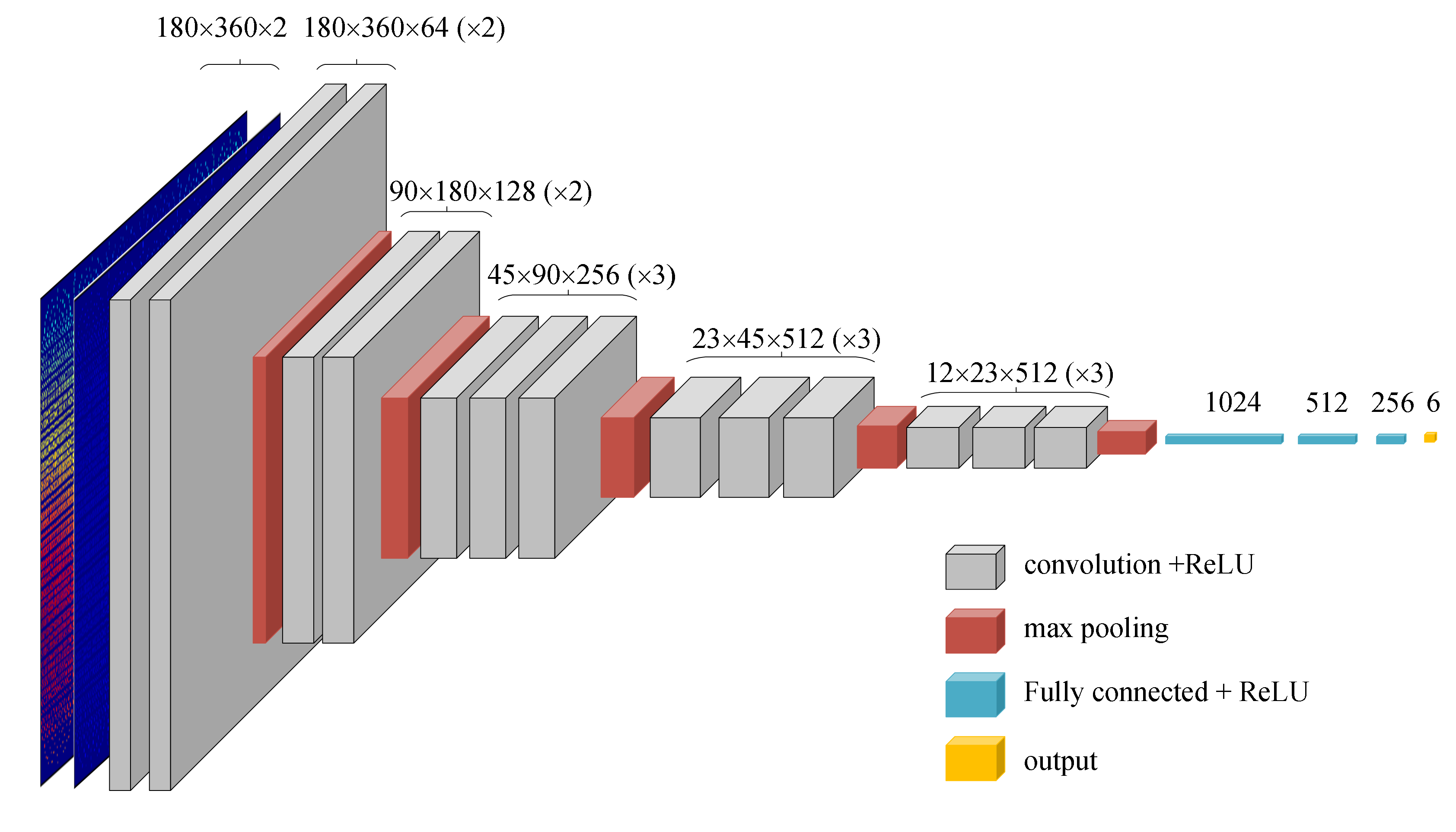
Figure 7: Convolutional neural networks configuration adapted from VGGNet16, which is widely used to extract image features and image classification.

Loss function

The loss function is an indicator used to measure the difference between the model prediction and the true values which is used for the optimization of the model. The loss function used in this study, shown in Eq. 4, consists of two terms. The first term represents the error between the true label and predicted label of the muon track. The second term provides a regularization penalty phaisangittisagul2016analysis which acts to avoid overfitting of the model and contains $\lambda$ coefficient scale and a summation over the weights of the model $W_{j}$.

$$Loss=\sum_{i}(||\vec{track}^{\scriptsize\textrm{predict}}_{i}-\vec{track}^{\scriptsize\textrm{truth}}_{i}||^{2})+\sum_{j}\lambda||W_{j}||^{2}$$ (4)

The training process acts to reduce the loss function resulting in the predicted values approaching closer to the actual values. With muon reconstruction this corresponds to improving the spatial and angular resolution of the reconstruction.

Implementation and training

The network used in this article is implemented using the TensorFlow Abadi:2016kic open source framework and its Python interface. The hardware environment uses the NVIDIA Tesla V100 GPU. Network training uses 2 GPUs for parallel computing. Using Mini-Batch orr2003neural training strategy, the size of batch is 256 (256 samples are trained at the same time in each iteration), which is divided into two smaller batches and computed in parallel on 2 GPUs. Two GPUs provides a speedup of 1.7 times, as compared to using a single GPU. On a system equipped with two NVIDIA Tesla V100 GPUs, training a single network took about 70 hours depending on the architecture.

The training neural network uses the stochastic gradient descent method to calculate the gradient of the loss function in the weight parameter space, and then advances the weight parameters by a certain step in the direction of the negative gradient. After reaching the set number of iterations or the set error accuracy, the weight parameter is considered to have reached the optimum position where the loss function is the smallest. The step size in the gradient descent process is the learning rate. After some studies, the following optimized learning rate schedule is used: the learning rate is initialized to be 0.1 at the beginning of training and is decreased by a factor of 10 after each 50,000 training steps.

The loss values from training dataset and validation dataset are monitored during the network training. It is found that after 200,000 training steps, the loss values from training dataset and validation dataset are almost stable which means the network has reached the optimized status. Besides, during the training the loss from validation dataset decreases smoothly which indicates the training process does not suffer from overfitting (a phenomenon that a model has over-learned features specific to the training dataset that are not present in general datasets, which is harmful to the model).

Performance study

Reconstruction resolution and efficiency

The network proposed in this paper is separately trained on dataset “Training TT$\_$rot” and “Training MC” which is used for verifying the rotation method. After training, they are tested by dataset “Testing MC” for performance analysis. After trying some fitting functions for the distribution of $\alpha$, it is found that the fitting effect is good using the improved Landau function Cao:2010zzd $f(x)=p_{0}\exp(-p_{3}(\lambda+\exp(-\lambda)))$, where $\lambda=\frac{x-p_{1}}{p_{2}}$. The full width at half maximum (FWHM) of the fitted distribution is defined as the resolution of $\alpha$. The distribution of reconstructed $\Delta$D is fitted to a Gaussian function and its resolution is obtained from the sigma of the Gaussian.

Figure 8 (a) and (b) show the distributions and fitting results of $\alpha$ and $\Delta$D obtained by using “Training TT$\_$rot” as training data when the distance of muon track from the center of CD ($D_{mc}$) is 14.7 m-16.7 m. Good fits have been achieved for both the angular and spatial resolutions.

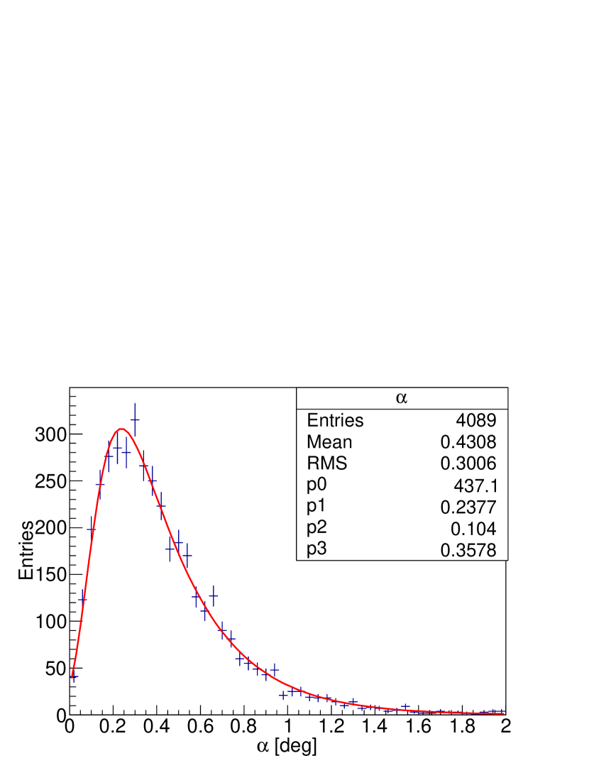
(a) $\alpha$ distribution fitted by improved Landau function

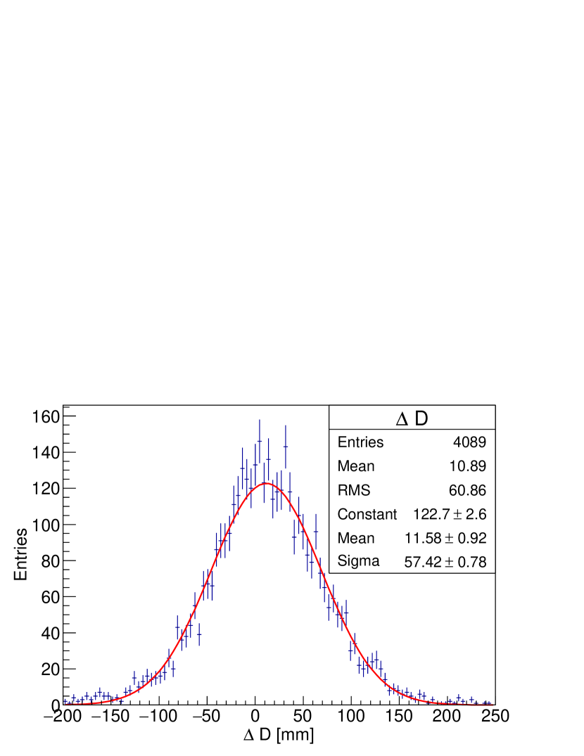
(b) $\Delta$D distribution fitted by Gaussian function

Figure 8: $\alpha$ and $\Delta$D reconstructed from the events where the track is 14.7 m to 16.7 m from the center of CD

Figure 9 shows how the reconstructed $\alpha$ and $\Delta$D vary with $D_{mc}$. Comparing the performance obtained when training with the “Training TT$\_$rot” and “Training MC” datasets we observe:

• For the “Training TT$\_$rot” dataset the angular bias of $\alpha$ is less than 0.4 degrees, and the spatial bias of $\Delta$D is less than 3 cm. Also the results from the “Training TT$\_$rot” and “Training MC” are very similar suggesting that using TT reconstructed tracks with experiment data will provide a realistic way to train the network that does not depend on the simulation.

• The sigma (or resolution) of $\alpha$ and $\Delta$D increases with the $D_{mc}$. When the muon track is close to the edge of CD, the position of the incident point and the exit point are very close to each other which makes an accurate reconstruction of the track direction difficult. This degradation of angular reconstruction at large distances from the CD center is also seen with the existing muon reconstruction methodsGenster:2018caz ; Zhang:2018kag . Overall, the angular resolution is better than 0.6 degrees and the spatial resolution is better than 10 cm.

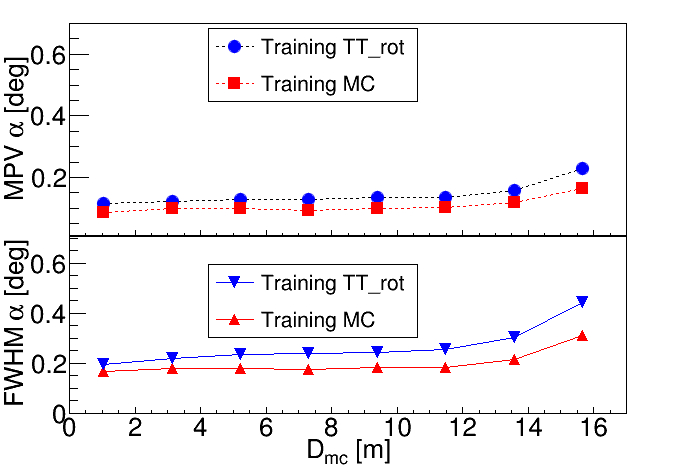
(a) Most probable value(MPV) and full width at half maxima(FWHM) value of $\alpha$ versus $D_{mc}$

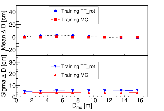
(b) Mean and sigma value of $\Delta$D versus $D_{mc}$

Figure 9: Performances of reconstruction with various training data.

In order to understand our muon reconstruction method better, figure 10 provides another check of the muon reconstruction performance obtained with the dataset “Training TT$\_$rot”. Here the $\Delta r$ resolution is expressed as FWHM of $\Delta r=|\vec{r}^{\scriptsize\textrm{predict}}_{\scriptsize\textrm{in}}-\vec{r}^{\scriptsize\textrm{truth}}_{\scriptsize\textrm{in}}|$ which means the difference between the true and predicted positions of the muon injection point at LS surface. The direction resolution is showed by the sigma of the distribution of $\Delta\theta$ and $\Delta\phi$ which express the differences of $\theta$ angles and $\phi$ angle between the reconstructed and true direction of muon track, respectively. Form figure 10, one can see the results are normal and there are no anomalies.

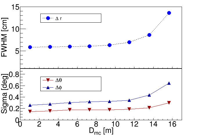
Figure 10: Reconstruction spatial resolution and angular resolution

The track reconstruction efficiency is defined as the ratio of well reconstructed tracks to all tracks, with tracks regarded as well reconstructed when the deviations of all parameters are less than five times their standard deviations. Figure 11 presents the reconstruction efficiency for a range of track distances from the CD center. For distances of less than 14 m the tracking efficiency is greater than 95%, dropping to 86% for tracks at the edge of the CD.

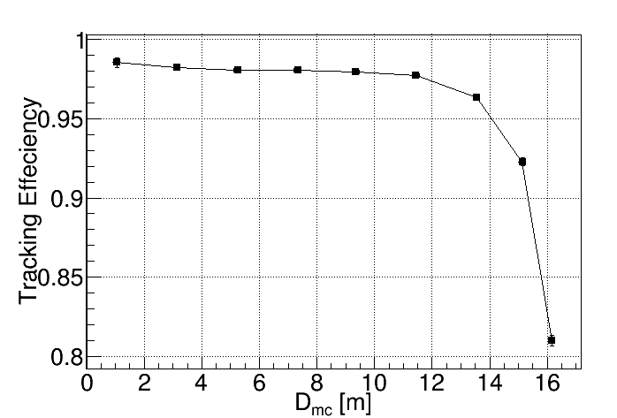
Figure 11: Reconstruction efficiency for various muon track distances to the CD center.

Reconstruction time cost

The time cost of muon reconstruction using three different approaches is presented in Table 3. The time for the CPU implementation of the neural network method presented in this paper is found to be improved by more than a factor of two compared to the fastest light method. The GPU implementation of the neural network method provides a huge processing speed improvement of a factor of one hundred compared to the CPU implementation.

Table 3: Reconstruction speed.

Method	Hardware	Time per event [ms]
Fastest Light	CPU E5-2650 v4	5000
Neutral Network (batch size=1)	CPU E5-2650 v4	2000
Neutral Network (batch size=1)	GPU Tesla V100	20

Discussion

The muon reconstruction accuracy of the deep learning model largely relies on the amount and the diversity of data available during training. Applying rotation to injected muon tracks can be effectively used to augment the training data. However the disadvantage with the rotation method is that it could lead to small changes in geometry that can cause a muon track represented by an image to lose part of its original features, which might possibly degrade the performance of reconstruction. Studies show that the performance discrepancy between the rotation method and the MC truth method is at the level of a few percent, which is still in an acceptable range. In order to further improve the performance of the CNN model, more sophisticated data augmentation method, such as data augmentation using GANs tanaka2019data , can be investigated and potentially used to generate artificial training data in the future.

The muon reconstruction results presented in the previous section are obtained in an ideal scenario. With the real experimental data, there are many factors that could possibly degrade the performance of the model. The possible influence factors are as follows: the dark noise created by the PMT, electronics saturation, the deformation of acrylic sphere etc.

When the experiment starts data taking, it takes time to complete the tuning of Monte Carlo simulation to make the simulation consistent with the data. During this period, deep learning model can be obtained by training with the augmented data sample. As soon as the reliable simulation data are available, the training can move to use the full simulation data.

Conclusion

In this study a deep learning convolutional neural network approach is applied to muon track reconstruction in the JUNO central detector. Achieving good agreement between the real JUNO experimental data and the simulated MC data is expected to require extensive efforts to develop a detailed understanding of many small effects corresponding to improvements to the models of the scintillation, re-emission, photon propagation into PMTs and the electronics. Reconstruction techniques which are not dependent on the availability of finely tuned simulation data are highly beneficial. In this study the track information reconstructed by the top tracker is used for network training instead of relying on Monte Carlo truth information. Due to the limited angular coverage of the top tracker a randomized event rotation technique has been developed which succeeds to generate sufficient training data by making the assumption of rotational symmetry. This dataset was used to train a convolutional neural network with promising reconstruction performance. The reconstruction efficiency is higher than 95% with the distance less than 14 meters of the track to CD center. The angular resolution is better than 0.6 degrees and the spatial resolution is better than 10 cm, and these results demonstrate that muon reconstruction a convolutional neural network is able to provide an performance that meets the requirements. Compared to existing methodsZhang:2018kag , the CNN model does not need to introduce additional real data correction. In addition, the GPU implementation of the technique has the advantage of a processing speed more than 100 times faster than conventional techniques.

References

- (1) Z. Djurcic et al. (JUNO Collaboration), arXiv:1508.07166
- (2) C. Genster, M. Schever, L. Ludhova, M. Soiron, A. Stahl and C. Wiebusch, arXiv:1906.01912 doi:10.1088/1748-0221/13/03/T03003
- (3) K. Zhang, M. He, W. Li and J. Xu,arXiv:1803.10407 doi:10.1007/s41605-018-0040-8
- (4) O. Russakovsky, J. Deng, H. Su, J. Krause, S. Satheesh, S. Ma et al., arXiv:1409.0575
- (5) R. Girshick, J. Donahue, T. Darrell, and J. Malik. Rich feature hierarchies for accurate object detection and semantic segmentation. In CVPR, 2014
- (6) J. Long, E. Shelhamer, and T. Darrell. Fully convolutional networks for semantic segmentation. In CVPR, 2015.
- (7) G. Kasieczka, T. Plehn, M. Russell and T. Schell. arXiv:1701.08784 doi:10.1007/JHEP05(2017)006
- (8) P. Baldi, K. Bauer, C. Eng, P. Sadowski and D. Whiteson,. arXiv:1603.09349 doi:10.1103/PhysRevD.93.094034
- (9) W. Bhimji, S. A. Farrell, T. Kurth, M. Paganini, Prabhat and E. Racah, arXiv:1711.03573 doi:10.1088/1742-6596/1085/4/042034
- (10) A. Aurisano, A. Radovic, D. Rocco, A. Himmel, M. D. Messier, E. Niner, G. Pawloski, F. Psihas, A. Sousa and P. Vahle, arXiv:1604.01444 doi:10.1088/1748-0221/11/09/P09001
- (11) X. Huang, et al., offline Data Processing Software for the JUNO Experiment, PoS ICHEP2016 (2017) 1051. doi:10.22323/1.282.1051.
- (12) T. Lin et al. [JUNO], J. Phys. Conf. Ser. 898, no.4, 042029 (2017) doi:10.1088/1742-6596/898/4/042029 [arXiv:1702.05275 [physics.ins-det]].
- (13) J. Allison, et al., Recent developments in geant4, NIM A 835 (2016) 186-225. doi: 10.1016/j.nima.2016.06.125.
- (14) V. A. Kudryavtsev, Comput. Phys. Commun. 180, 339-346 (2009) doi:10.1016/j.cpc.2008.10.013 [arXiv:0810.4635 [physics.comp-ph]].
- (15) M. Guan, M. C. Chu, J. Cao, K. B. Luk and C. Yang, arXiv:1509.06176.
- (16) K. Simonyan and A. Zisserman. Very deep convolutional networks for large-scale image recognition. In ICLR, 2015. 1, 5
- (17) D. Scherer, A. Muller and S. Behnke, Evaluation of pooling operations in convolutional architectures for object recognition, in proceedings of The International Conference on Artificial Neural Networks (ICANN), Thessaloniki, Greece, 15–18 September 2010, Springer.
- (18) K. K. Pal and K. S. Sudeep, Preprocessing for image classification by convolutional neural networks, IEEE, 2016, pp. 1778-1781, doi: 10.1109/RTEICT.2016.7808140.
- (19) E. Phaisangittisagul, An analysis of the regularization between L2 and dropout in single hidden layer neural network[C]. IEEE, 2016: 174-179.
- (20) M. Abadi, et al., Tensorflow: Large-scale machine learning on heterogeneous distributed systems (2015). arXiv:1603.04467
- (21) Y. LeCun, L. Bottou, G. B. Orr and K. R. Müller, Neural Networks: Tricks of the Trade. Springer Berlin Heidelberg, 1998.
- (22) X. X. Cao, W. D. Li, R. A. Briere, C. L. Liu, Z. P. Mao, S. J. Chen, Z. Y. Deng, K. L. He, X. T. Huang and B. Huang, et al. Chin. Phys. C 34 (2010), 1852-1859 doi:10.1088/1674-1137/34/12/012
- (23) F. H. K. dos Santos Tanaka and C. Aranha (2019). Data Augmentation Using GANs. ArXiv, abs/1904.09135.