Three-particle ladder method for photoinduced dynamics of organic molecules

Photoinduced dynamics of organic molecules using nonequilibrium Green’s functions with second-Born, $GW$, $T$-matrix and three-particle ladder correlations

Abstract

The ultrafast hole dynamics triggered by the photoexcitation of molecular targets is a highly correlated process even for those systems, like organic molecules, having a weakly correlated ground state. We here provide a unifying framework and a numerically efficient matrix formulation of state-of-the-art non-equilibrium Green’s function (NEGF) methods like second-Born as well as $GW$ and $T$-matrix without and with exchange diagrams. Numerical simulations are presented for a paradigmatic, exactly solvable molecular system and the shortcomings of the established NEGF methods are highlighted. We then develop a NEGF scheme based on the Faddeev treatment of three-particle correlations; the exceptional improvement over established methods is explained and demonstrated. The Faddeev NEGF scheme scales linearly with the maximum propagation time, thereby opening prospects for femtosecond simulations of large molecules.

I Introduction

The study of nonequilibrium phenomena in correlated materials has recently become one of the most active and exciting branches of atomic, molecular and condensed matter physics. This is largely due to advances in light sources and time-resolved spectroscopies on the ultrashort time scales Zhang and Averitt (2014), which made it possible not only to observe and describe but also to design systems with new remarkable properties by coupling them to external electromagnetic fields Lépine et al. (2014). In a long time perspective they may lead to practical applications having a huge societal impact Kraus et al. (2018).

As an example, consider the quantum evolution of an organic molecule initially in its weakly correlated ground-state and then perturbed by an ultra-short (sub-fs) weak XUV pulse Calegari et al. (2014); Iablonskyi et al. (2017); Lara-Astiaso et al. (2018); Hervé et al. (2020). The target molecule undergoes a transition to an excited one-hole state through the emission of a single electron. The resulting cationic state can no longer be characterized as weakly correlated. In fact, immediately after the excitation quantum scattering processes mediated by the Coulomb interaction start to roll. They promote the decay of the left behind hole into a two-hole and one-particle ($2h$-$1p$) state. Thus, in contrast to the initial non-degenerate ground state, the system is now in a superposition of a large number of quasi-degenerate states whose energies and mutual interactions represent a formidable challenge for the theory. In particular, this is true for methods based on density functional theory as they rely on ground state correlations only. It is also a challenge for wave-function methods. They can, in principle, deal with multi-configurational ionized states (static correlations) Kuleff et al. (2005); Szalay et al. (2011); Popova-Gorelova et al. (2016) and systematically treat $2h$-$1p$, $3h$-$2p$, etc. configurations, thus making the approach accurate and predictive for small molecular systems. However, the inclusion of dynamical correlations (quasi-particle dressing in physics therminlogy) remains a difficult numerical task.

Other challenges for the theory include the treatment of large molecular systems, where nuclear and collective electronic excitations emerge as important scattering channels Schüler et al. (2016); Usenko et al. (2016), as well as the description of processes with a variable number of particles as in transport Cuniberti et al. (2005); Cuevas and Scheer (2010) and photoemission experiments Cardona and Ley (1978); Freericks et al. (2009); Pavlyukh et al. (2015). Methods that can deal with all theses ingredients on equal footing are still in their infancy; developments in the realm of wave-function expansions Ruberti et al. (2014, 2018a, 2018b); Pathak et al. (2020) and time-dependent DFT are certainly foreseeable Andreussi et al. (2015); Nisoli et al. (2017).

The nonequilibrium Green’s function (NEGF) theory Stefanucci and van Leeuwen (2013); Balzer (2013) is another fertile playground for the development of efficient methods. Its main variable, namely the single-particle Green’s function, naturally appears in the observables characterizing the aforementioned phenomena, and the inclusion of static and dynamical electronic correlations as well as interactions with other quasiparticles of bosonic nature, such as plasmons and vibrational modes, is possible through the exact resummation of diagrammatic expansions to infinite order in the interactions strength.

The NEGF versatility, however, comes at the cost of dealing with two-times correlators. The time-evolution of any quantum systems is described by the so called Kadanoff-Baym equations (KBE) Stefanucci and van Leeuwen (2013); Balzer (2013) for the Green’s function. The KBE are nonlinear first-order integro-differential equations scaling cubically with the physical propagation time, thereby making it difficult to resolve small energy scales associated with phonons, magnons, etc. A less severe quadratic scaling can be achieved by means of the so-called Generalized Kadanoff-Baym Ansatz (GKBA) Lipavský et al. (1986) which allows for reducing the KBE to a single equation of motion for the one-particle density matrix Karlsson et al. (2018). Recent applications of the NEGF + GKBA approach include the nonequilibrium dynamics Hermanns et al. (2014); Schlünzen et al. (2016) and many-body localization Bar Lev and Reichman (2014) of Hubbard clusters, time-dependent quantum transport Latini et al. (2014); Cosco et al. (2020); Tuovinen et al. (2021), real-time description of the Auger decay Covito et al. (2018), excitonic insulators out of equilibrium Tuovinen et al. (2020), equilibrium absorption of sodium clusters Pal et al. (2011), transient absorption Perfetto et al. (2015a, b); Sangalli et al. (2016); Pogna et al. (2016) and carrier dynamics Sangalli and Marini (2015); Perfetto et al. (2016) of semiconductors. A tremendous progress has been recently achieved in further reducing the scaling to the ideal linear law and establishing that the method is applicable for state-of-the-art diagrammatic approximations like the second-Born (2B), $GW$ and $T$-matrix (both in the $ph$ and $pp$ channels) Joost et al. (2020). These approximations have been extensively tested in the past for model and realistic systems in the neutral state, both by solving full Kadanoff-Baym equations Dahlen and van Leeuwen (2007); Myöhänen et al. (2008, 2009); Puig von Friesen et al. (2010); Friesen et al. (2010); Säkkinen et al. (2012) and by using GKBA Joost et al. (2020); Tuovinen et al. (2020); Murakami et al. (2020). However, they loose accuracy in the description of photoionization-induced dynamics even for systems having a weakly correlated ground state.

Let us return to our initial picture of the $1h\rightarrow 2h$-$1p$ scattering in photoexcited molecular targets. In a realistic scenario one has to deal with recurrent scatterings of this kind. Mathematically this is treated by the resummation of certain classes of Feynman diagrams. One may focus on the fate of one particle and one hole in the final state and disregard other interactions, schematically indicated as $h\rightarrow(p+h)+h$. Depending on which hole $h$ is paired with the particle $p$ in the final state we end up with either the $GW$ approximation or the $T$-matrix approximation in the $ph$ channel (henceforth $T^{ph}$). Alternatively, one may elect to describe the interactions between two-holes (or particles) in the final channel, schematically indicated as $h\rightarrow(h+h)+p$, leading to the so-called $T$-matrix approximation in the $pp$ channel (henceforth $T^{pp}$) Pavlyukh et al. (2013). All these approximations treat either a hole or a particle as spectator, i. e., they ignore three-particle correlations. Such limitation has a profound impact in the description of fundamental physical processes. This is especially true in the presence of (near) degeneracies between the involved electronic states. In the case of the inter-valence hole migration the quasi-degeneracies are due to spin degrees of freedom. The multitude of spin-states in the $1h\rightarrow 2h$-$1p$ scattering scenario is not accounted for by the conventional $GW$ and $T$-matrices approximations.

In this work we apply all conventional approximations to study the inner-valence hole migration in the glycine molecule. The numerical simulations clearly show that none of these methods is capable to describe the quantum beating associated with transitions between different $2h$-$1p$ states. A resolution within NEGF is achievable by explicitly correlating the three-particle states. The so called three-particle ladder approximation has been first explored in the context of nuclear physics Barbieri and Dickhoff (2001) and it leads to the well known Faddeev equations Faddeev (1961); Ethofer and Schuck (1969). These equations have been applied to model Potthoff et al. (1994), atomic Barbieri et al. (2007) and small molecular systems Degroote et al. (2011). However, to the best of our knowledge, the Faddeev equations have never been investigated in the context of the NEGF formalism.

The main achievement of our work is the development of a NEGF+GKBA method based on the three-particle ladder diagrams. For the purpose of a self-contained exposition we first introduce the 2B, $GW$ and $T$-matrix approximations. In Sec. II we provide a simple and concise derivation of the equations of motion, cast the equations in a numerically efficient matrix form and highlight the common underlying mathematical structure of all these approximations. In Sec. III we present the full-fledged three-particle method, henceforth refered to as the Faddeev approximation. Its derivation relies on the extension of the GKBA to high-order Green’s functions. Conventional and Faddeev approximations are benchmarked against the exact photoinduced electron dynamics in the paradigmatic glycine molecule, finding an excellent agreement for the latter, see Section IV. Noteworthy, the numerical solution of the Faddeev-GKBA method scales linearly with the maximum propagation time. In Sec. V we recapitulate our finding and propose systems and experimental scenarios where the method is particularly relevant.

II Unifying formulation of the GKBA equations for state-of-the-art methods

Table 1: Definitions of the two-particle 2-rank tensors. The vertically grouped indices are combined into one super-index. Here $h\equiv h_{\text{HF}}$ for brevity.

Quantity	2B	$GW\;+(X)$	$T^{pp}\;+(X)$	$T^{ph}\;+(X)$
$\bm{\mathcal{G}}$	$\bm{\mathcal{G}}_{\begin{subarray}{c}13\\ 24\end{subarray}}=\mathcal{G}_{4132}$	$\bm{\mathcal{G}}_{\begin{subarray}{c}13\\ 24\end{subarray}}=\mathcal{G}_{4132}$	$\bm{\mathcal{G}}_{\begin{subarray}{c}13\\ 24\end{subarray}}=\mathcal{G}_{1234}$	$\bm{\mathcal{G}}_{\begin{subarray}{c}13\\ 24\end{subarray}}=\mathcal{G}_{1432}$
$\mathbfit{h}$	$\mathbfit{h}_{\begin{subarray}{c}13\\ 24\end{subarray}}=h_{13}\delta_{42}-\delta_{13}h_{42}$	$\mathbfit{h}_{\begin{subarray}{c}13\\ 24\end{subarray}}=h_{13}\delta_{42}-\delta_{13}h_{42}$	$\mathbfit{h}_{\begin{subarray}{c}13\\ 24\end{subarray}}=h_{13}\delta_{24}+\delta_{13}h_{24}$	$\mathbfit{h}_{\begin{subarray}{c}13\\ 24\end{subarray}}=h_{13}\delta_{42}-\delta_{13}h_{42}$
$\mathbfit{v}$	$\mathbfit{v}_{\begin{subarray}{c}13\\ 24\end{subarray}}=v_{1432}$	$\mathbfit{v}_{\begin{subarray}{c}13\\ 24\end{subarray}}=v_{1432}$	$\mathbfit{v}_{\begin{subarray}{c}13\\ 24\end{subarray}}=v_{1243}$	$\mathbfit{v}_{\begin{subarray}{c}13\\ 24\end{subarray}}=v_{1423}$
$\mathbfit{w}$	$\mathbfit{w}_{\begin{subarray}{c}13\\ 24\end{subarray}}=v_{1432}-v_{1423}$	$\mathbfit{w}_{\begin{subarray}{c}13\\ 24\end{subarray}}=v_{1432}-(v_{1423})$	$\mathbfit{w}_{\begin{subarray}{c}13\\ 24\end{subarray}}=v_{1243}-(v_{1234})$	$\mathbfit{w}_{\begin{subarray}{c}13\\ 24\end{subarray}}=v_{1423}-(v_{1432})$
$\bm{\mathit{\rho}}^{<}$	$\bm{\mathit{\rho}}^{<}_{\begin{subarray}{c}13\\ 24\end{subarray}}=\rho^{<}_{13}\rho^{>}_{42}$	$\bm{\mathit{\rho}}^{<}_{\begin{subarray}{c}13\\ 24\end{subarray}}=\rho^{<}_{13}\rho^{>}_{42}$	$\bm{\mathit{\rho}}^{<}_{\begin{subarray}{c}13\\ 24\end{subarray}}=\rho^{<}_{13}\rho^{<}_{24}$	$\bm{\mathit{\rho}}^{<}_{\begin{subarray}{c}13\\ 24\end{subarray}}=\rho^{<}_{13}\rho^{>}_{42}$
$\bm{\mathit{\rho}}^{>}$	$\bm{\mathit{\rho}}^{>}_{\begin{subarray}{c}13\\ 24\end{subarray}}=\rho^{>}_{13}\rho^{<}_{42}$	$\bm{\mathit{\rho}}^{>}_{\begin{subarray}{c}13\\ 24\end{subarray}}=\rho^{>}_{13}\rho^{<}_{42}$	$\bm{\mathit{\rho}}^{>}_{\begin{subarray}{c}13\\ 24\end{subarray}}=\rho^{>}_{13}\rho^{>}_{24}$	$\bm{\mathit{\rho}}^{>}_{\begin{subarray}{c}13\\ 24\end{subarray}}=\rho^{>}_{13}\rho^{<}_{42}$
$a$	$0$	$-1$	$1$	$1$

Let us start from a generic fermionic Hamiltonian

$$\hat{H}(t)=\sum_{ij}h_{ij}(t)\hat{d}_{i}^{\dagger}\hat{d}_{j}+\frac{1}{2}\sum_{ijmn}v_{ijmn}(t)\hat{d}_{i}^{\dagger}\hat{d}_{j}^{\dagger}\hat{d}_{m}\hat{d}_{n},$$ (1)

where $h_{ij}$ stands for the one-body part and $v_{ijmn}$ is the Coulomb interaction tensor, they are time-dependent in general. The time-dependence in $h_{ij}(t)$ originates, for instance, from the coupling to external fields, whereas the time-dependence in $v_{ijmn}(t)$ could be due to the adiabatic switching protocol adopted to generate a correlated initial state. Below, we skip the time-arguments if they are not essential for the discussion. The indices $i,\,j$, etc. comprise a spin index and an orbital index which (without any loss of generality) is associated with some localized basis functions, but it is straightforward to reformutate the equations in, e. g., plane-wave basis or any other suitable basis. In this work we consider a spin symmetric single-particle Hamiltonian and a spin-independent interaction. Making explicit the spin-dependence this implies that $h_{i\sigma_{1}j\sigma_{2}}=\delta_{\sigma_{1}\sigma_{2}}h_{ij}$ and

$$v_{i\sigma_{1}j\sigma_{2}m\sigma_{3}n\sigma_{4}}=\delta_{\sigma_{1}\sigma_{4}}\delta_{\sigma_{2}\sigma_{3}}v_{ijmn}.$$ (2)

The lesser and the greater Green’s functions (GFs) are defined as

$$G^{<}_{ij}(t,t^{\prime}) =+\mathrm{i}\big{\langle}\hat{d}_{j}^{\dagger}(t^{\prime})\hat{d}_{i}(t)\big{\rangle},$$ (3a)

$$G^{>}_{ij}(t,t^{\prime}) =-\mathrm{i}\big{\langle}\hat{d}_{i}(t)\hat{d}_{j}^{\dagger}(t^{\prime})\big{\rangle},$$ (3b)

and fulfill the symmetry relation $G^{\lessgtr}(t_{1},t_{2})=-\left[G^{\lessgtr}(t_{2},t_{1})\right]^{\dagger}$. They carry information on the single-particle spectra and occupations. The generalized Kadanoff-Baym Ansatz (GKBA) Lipavský et al. (1986) factorizes these two independent ingredients, see Appendix A,

$$G^{\lessgtr}(t_{1},t_{2}) =-G^{R}(t_{1},t_{2})\rho^{\lessgtr}(t_{2})+\rho^{\lessgtr}(t_{1})G^{A}(t_{1},t_{2})$$ (4)

so that the greater/lesser density matrices become our main single-time variables

$$\rho_{ij}^{\lessgtr}(t)=-\mathrm{i}G^{\lessgtr}_{ij}(t,t)\quad\quad[\rho^{>}_{ij}=\rho^{<}_{ij}-\delta_{ij}].$$ (5)

Using the GKBA the KBE are reduced to an equation of motion for the density matrix

$$\frac{d}{dt}\rho^{<}(t) =-\mathrm{i}\big{[}h_{\text{HF}}(t),\rho^{<}(t)\big{]}-\left(I(t)+I^{\dagger}(t)\right)$$ (6)

provided that the retarded ($G^{R}$) and advanced ($G^{A}$) Green’s functions are approximated as functional of $\rho^{<}$. In this work we consider the Hartree-Fock functional form

$$G^{R}(t,t^{\prime})=-\mathrm{i}\theta(t-t^{\prime})T\left\{e^{-\mathrm{i}\int_{t^{\prime}}^{t}d\tau\,h_{\text{HF}}(\tau)}\right\},$$ (7)

and hence $G^{\rm A}(t,t^{\prime})=[G^{\rm R}(t^{\prime},t)]^{{\dagger}}$.

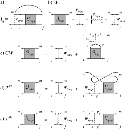
Figure 1: Diagrammatic representation of the Eq. (9) for the scattering term.

In Eqs. (6) and (7)

$$h_{\text{HF},ij}(t)=h_{ij}(t)+\sum_{mn}[v_{imnj}-v_{imjn}]\rho^{<}_{nm}(t)$$ (8)

is the Hartree-Fock (HF) Hamiltonian, which is a functional of $\rho^{<}$. The so called collision integral $I(t)$ in Eq. (6) does therefore account for electronic correlations and through the GKBA and Eq. (7) it too is a functional of $\rho^{<}$, see below. The ultimate goal for numerics is to compute the collision integral in the most accurate and efficient fashion. Its exact form follows straightforwardly from the first equation of the Martin-Schwinger hierarchy and it involves the two-particle Green’s function (2-GF) $\mathcal{G}$ at equal times

$$I_{lj}(t) =-\mathrm{i}\sum_{imn}v_{lnmi}(t)\mathcal{G}_{imjn}(t).$$ (9)

The diagrammatic expression of Eq. (9) is shown in Fig. 1 (a).

In this Section we evaluate the collision integral in the diagrammatic approximation $d=$ 2B, see Fig. 1 (b), as well as $d=GW+(X)$, $T^{ph}+(X),\,T^{pp}+(X)$, see Fig. 1 (c-e). For the latter approximations the addition of exchange ($X$) simply amounts in solving the Bethe-Salpeter equations of Fig. 1 (c-e) with an interaction line $w_{imnj}=v_{imnj}-v_{imjn}$. In 2B the use of $w$ allows for writing the direct and exchange diagrams in terms of a diagram only, see again Fig. 1 (b). Depending on the approximation $d$ we find it convenient to rewrite Eq. (9) in different, yet equivalent, forms

$$I_{lj}(t) =-\mathrm{i}\sum_{imn}v^{(d)}_{\begin{subarray}{c}lm\\ in\end{subarray}}(t)\mathcal{G}^{(d)}_{\begin{subarray}{c}mj\\ ni\end{subarray}}(t)$$ (10)

where the relation between the one-particle 4-rank tensors $v$, $\mathcal{G}$ and the two-particle 2-rank tensors $v^{(d)}$, $\mathcal{G}^{(d)}$ is provided in Table 1. To distinguish matrices (2-rank tensors) in the two-particle space from matrices or tensors in the one-particle space we use bold letters for the former. In the following subsections we show that the GKBA expression for the 2-GF has the following compact form for all approximations (omitting the dependence on $d$)

$$\bm{\mathcal{G}}(t)=\mathrm{i}\int_{t_{0}}^{t}\!\!dt^{\prime}\,\mathbfit{\Pi}^{R}(t,t^{\prime})\bm{\mathit{\Psi}}(t^{\prime})\mathbfit{\Pi}^{A}(t^{\prime},t),$$ (11)

where the initial time $t_{0}=0$, without any loss of generality. Thus $\bm{\mathcal{G}}$ is the integral of a product between ($d$-dependent) time-dependent matrices in the two-particle space. The ($d$-dependent) matrix

$$\bm{\mathit{\Psi}}(t)\equiv\bm{\mathit{\rho}}^{>}(t)\mathbfit{w}(t)\bm{\mathit{\rho}}^{<}(t)-\bm{\mathit{\rho}}^{<}(t)\mathbfit{w}(t)\bm{\mathit{\rho}}^{>}(t)$$ (12)

is a simple product between the time-dependent matrices $\bm{\mathit{\rho}}^{\lessgtr}$ and $\mathbfit{w}$ defined in Table 1. The ($d$-dependent) retarded propagator $\mathbfit{\Pi}^{R}(t,t^{\prime})=[\mathbfit{\Pi}^{A}(t^{\prime},t)]^{{\dagger}}$ satisfies for any $t>t^{\prime}$ the differential equation

$$\mathrm{i}\frac{d}{dt}\mathbfit{\Pi}^{R}(t,t^{\prime})=\big{[}\mathbfit{h}(t)+a\,\mathbfit{w}(t)\bm{\mathit{\rho}}^{\Delta}(t)\big{]}\mathbfit{\Pi}^{R}(t,t^{\prime}),$$ (13)

with the boundary condition

$$\mathrm{i}\mathbfit{\Pi}^{R}(t^{+},t)=\mathbb{1}\times\left\{\begin{array}[]{rl}-1,&\quad d={\rm 2B},\;GW;\\ 1,&\quad d=T^{ph},\;T^{pp}.\end{array}\right.$$ (16)

The matrix $\mathbfit{h}$ as well as the constant $a$ are given in Table 1 whereas

$$\bm{\mathit{\rho}}^{\Delta}(t)\equiv\bm{\mathit{\rho}}^{>}(t)-\bm{\mathit{\rho}}^{<}(t).$$ (17)

The equation of motion for the 2-GF Schlünzen et al. (2020); Joost et al. (2020) follows directly from Eq. (13)

$$\mathrm{i}\frac{d}{dt}\bm{\mathcal{G}}(t)=-\bm{\mathit{\Psi}}(t)+\left[\mathbfit{h}(t)+a\bm{\mathit{\rho}}^{\Delta}(t)\mathbfit{w}(t)\right]\bm{\mathcal{G}}(t)\\ -\bm{\mathcal{G}}(t)\left[\mathbfit{h}(t)+a\mathbfit{w}(t)\bm{\mathit{\rho}}^{\Delta}(t)\right].$$ (18)

The coupled differential equations (6) and (18) form the essence of the NEGF+GKBA method for all the approximations in Tab. 1. The numerical solution of these equations scales linearly with the propagation time. The concise derivation of such unifying formulation is made possible by the diagrammatic structure of the 2-GF which takes into account only 2-particle correlations (in $p$-$p$ or $p$-$h$ channels), see again Fig. 1 (c-e). We can then order the indices, see Table 1, in such a way as to construct RPA-like equations in the respective channels. The contraction over the pair of indices translates in our notation to a matrix product while the particle permutation symmetry is taken into account by the constant $a$. The 2B approximation is the lowest order term of all the correlated methods, $GW$ and $T$-matrix, when exchange is added. Accordingly, the 2B equations (now expressed in the $GW$ index convention) can be equivalently formulated using the $T$-matrix index conventions – this point is expanded in Section II.1. We also observe that

$$\bm{\mathcal{G}}^{\dagger} =\bm{\mathcal{G}}, \mathbfit{v}^{\dagger} =\mathbfit{v}, \mathbfit{w}^{\dagger} =\mathbfit{w}, \mathbfit{h}^{\dagger} =\mathbfit{h}, {\bm{\mathit{\rho}}^{\gtrless}} =\bm{\mathit{\rho}}^{\gtrless},$$ (19)

as it follows directly from the symmetry properties

$$v_{1234} =v_{4321}^{*}=v_{2143},$$ (20a)

$$\mathcal{G}_{1234} =\mathcal{G}_{3421}^{*}=\mathcal{G}_{2143}.$$ (20b)

In the remainder of the Section we present the derivation of Eq. (11). We point out, however, that it is not necessary to go through the derivation in order to follow the Faddeev approximation in Section III.

II.1 Second Born approximation

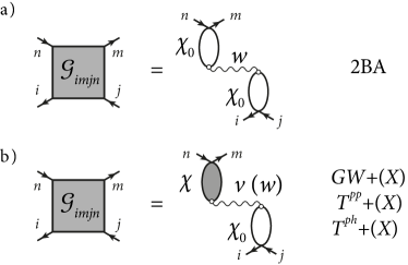
Figure 2: Diagrammatic representation of Eq. (21) (a) and Eq. (II.2) (b) for the two-particle Green’s function in terms of the RPA $\bm{\mathit{\chi}}$ and noninteracting $\bm{\mathit{\chi}}^{0}$ response functions.

Let us start with the simplest case, where the collision integral is given by its second-order (in $v$) expression — therefore the name. The equal-time 2-GF can be expressed as the convolution of two response functions $\bm{\mathit{\chi}}^{0}$, see Fig. 2 (a),

$$\bm{\mathcal{G}}(t)=-\mathrm{i}\int_{0}^{t}\!\!dt^{\prime}\Big{\{}\bm{\mathit{\chi}}^{0,>}(t,t^{\prime})\mathbfit{w}(t^{\prime})\bm{\mathit{\chi}}^{0,<}(t^{\prime},t)-(>\leftrightarrow<)\Big{\}}.$$ (21)

As already pointed out, in 2B there is a freedom in selecting the index convention. Let us define three different response functions as matrices in the two-particle space

$$\chi^{0,\lessgtr}_{\begin{subarray}{c}13\\ 24\end{subarray}}(t,t^{\prime})=\mathrm{i}\left\{\begin{array}[]{ll}-G^{\lessgtr}_{13}(t,t^{\prime})G^{\gtrless}_{42}(t^{\prime},t),&\quad GW\\[6.0pt] +G^{\lessgtr}_{13}(t,t^{\prime})G^{\lessgtr}_{24}(t,t^{\prime}),&\quad T^{pp}\\[6.0pt] +G_{13}^{\lessgtr}(t,t^{\prime})G^{\gtrless}_{42}(t^{\prime},t),&\quad T^{ph}\end{array}\right..$$ (25)

Then the collision integral in Eq. (10) does not change if we consistently use for $\mathbfit{v}$, $\bm{\mathit{\chi}}^{0,\lessgtr}$ and $\mathbfit{w}$ the same index convention as described in Table 1.

Evaluating the noninteracting response functions with the GKBA in Eq. (4) we find

$$\bm{\mathit{\chi}}^{0,\lessgtr}(t,t^{\prime})=\mathbfit{P}^{R}(t,t^{\prime})\bm{\mathit{\rho}}^{\lessgtr}(t^{\prime})-\bm{\mathit{\rho}}^{\lessgtr}(t)\mathbfit{P}^{A}(t,t^{\prime}),$$ (26)

where, depending on the approximation $d=GW,\,T^{pp},\,T^{ph}$,

$$\mathbfit{P}^{R}_{\begin{subarray}{c}13\\ 24\end{subarray}}(t,t^{\prime}) =\begin{cases}+\mathrm{i}G_{13}^{R}(t,t^{\prime})G_{42}^{A}(t^{\prime},t),&GW\\[4.0pt] +\mathrm{i}G_{13}^{R}(t,t^{\prime})G_{24}^{R}(t^{\prime},t),&T^{pp}\\[4.0pt] -\mathrm{i}G_{13}^{R}(t,t^{\prime})G_{42}^{A}(t^{\prime},t),&T^{ph}\end{cases},$$ (27)

$$\mathbfit{P}^{A}(t,t^{\prime}) =\left[\mathbfit{P}^{R}(t^{\prime},t)\right]^{\dagger},$$ (28)

and the matrices $\bm{\mathit{\rho}}^{>}$ and $\bm{\mathit{\rho}}^{<}$ are defined in Table 1 for each diagrammatic approximation. Taking into account that $t^{\prime}\leq t$ in Eq. (21), substituting Eqs. (26) into it we arrive at

$$\bm{\mathcal{G}}(t)=\mathrm{i}\int_{0}^{t}\!\!dt^{\prime}\,\mathbfit{P}^{R}(t,t^{\prime})\bm{\mathit{\Psi}}(t^{\prime})\mathbfit{P}^{A}(t^{\prime},t).$$ (29)

Comparing this result with Eq. (11) we are left to prove that $\mathbfit{P}^{R}$ satisfies Eq. (13) with boundary condition in Eq. (16). The equation of motion for $\mathbfit{P}^{R}$ follows from the equation of motion of the retarded/advanced Green’s functions. According to Eq. (7) we have (repeated indices are summed over)

$$\mathrm{i}\frac{d}{dt}G^{R/A}_{ma}(t,t^{\prime}) =h_{mc}^{\text{HF}}(t)G^{R/A}_{ca}(t,t^{\prime})+\delta_{ma}\delta(t-t^{\prime}),$$ (30a)

$$-\mathrm{i}\frac{d}{dt^{\prime}}G^{R/A}_{ma}(t,t^{\prime}) =G^{R/A}_{mc}(t,t^{\prime})h_{ca}^{\text{HF}}(t^{\prime})+\delta_{ma}\delta(t-t^{\prime}).$$ (30b)

By defining the matrix $\mathbfit{h}$ in the two-particle space according to Table 1 we can then write for all cases and for $t>t^{\prime}$

$$\mathrm{i}\frac{d}{dt}\mathbfit{P}^{R}(t,t^{\prime}) =\mathbfit{h}(t)\mathbfit{P}^{R}(t,t^{\prime}),$$ (31)

which coincides with Eq. (13) when $d=$ 2B since in this case $a=0$. The initial conditions for $\mathbfit{P}^{R}$ can likewise be obtained by taking the equal time-limit of Eq. (27) and by using $G^{R}(t^{+},t)=-\mathrm{i}$ and $G^{A}(t,t^{+})=\mathrm{i}$:

$$\mathrm{i}\mathbfit{P}^{R}(t^{+},t) =\mathbb{1}\times\begin{cases}-1&GW;\\ +1&T^{pp},\,T^{ph}.\end{cases}$$ (32)

Using the $GW$ index convention (this is the convention used in Tab. 1 for 2B) we find the boundary condition of Eq. (16).

II.2 $GW$ and $T$-matrices approximation

Higher-order diagrammatic approximations for $\bm{\mathcal{G}}$ such as $GW$ and $T$-matrices with exchange require the notion of the RPA response functions $\bm{\mathit{\chi}}$ as depicted in Fig. 2 (b). For all the cases we can write

$$\bm{\mathcal{G}}(t)=-\mathrm{i}\int^{t}_{0}\!\!dt^{\prime}\Big{\{}\bm{\mathit{\chi}}^{>}(t,t^{\prime})\mathbfit{w}(t^{\prime})\bm{\mathit{\chi}}^{0,<}(t^{\prime},t$$ (33)

-(>↔<)},

where the non-interacting $\bm{\mathit{\chi}}^{0}$ has been defined in Eq. (25). To recover the more standard $GW$ and $T$-matrix approximations we can simply replace $\mathbfit{w}$ with $\mathbfit{v}$ in Eq. (II.2) and in the RPA equation for $\bm{\mathit{\chi}}$. We can also consider the exchange-only version of these approximations; in this case the replacement is $\mathbfit{w}\to\mathbfit{w}-\mathbfit{v}$. To reduce the voluminousness of the equations we introduce the two-time function $\mathbfit{w}(t,t^{\prime})=\mathbfit{w}(t)\delta(t-t^{\prime})$ and the shorthand notation

$$[a\cdot b](t,t^{\prime})=\int\!d\bar{t}\,a(t,\bar{t})b(\bar{t},t^{\prime}).$$ (34)

The Langreth rules then imply, see Appendix B,

$$\bm{\mathit{\chi}}^{\lessgtr}=(\bm{\delta}+\bm{\mathit{\chi}}^{R}\cdot\mathbfit{w})\cdot\bm{\mathit{\chi}}^{0,\lessgtr}\cdot(\mathbfit{w}\cdot\bm{\mathit{\chi}}^{A}+\bm{\delta})$$ (35)

with

$$\bm{\mathit{\chi}}^{R/A} =\bm{\mathit{\chi}}^{0,R/A}+\bm{\mathit{\chi}}^{0,R/A}\cdot\mathbfit{w}\cdot\bm{\mathit{\chi}}^{R/A},$$ (36a)

$$=\bm{\mathit{\chi}}^{0,R/A}+\bm{\mathit{\chi}}^{R/A}\cdot\mathbfit{w}\cdot\bm{\mathit{\chi}}^{0,R/A}.$$ (36b)

In the $GW$ case $\bm{\mathit{\chi}}$ is well-known as the density-density response function, of high relevance for the optical properties. Let us work out the expression of $\bm{\mathit{\chi}}$ when the Green’s function is evaluated using the GKBA.

By definition $\bm{\mathit{\chi}}^{0,R/A}(t,t^{\prime})=\pm\theta(\pm t\mp t^{\prime})[\bm{\mathit{\chi}}^{0,>}(t,t^{\prime})-\bm{\mathit{\chi}}^{0,<}(t,t^{\prime})]$. Hence from Eq. (26)

$$\bm{\mathit{\chi}}^{0,R}(t,t^{\prime}) =\mathbfit{P}^{R}(t,t^{\prime})\bm{\mathit{\rho}}^{\Delta}(t^{\prime}),$$ (37a)

$$\bm{\mathit{\chi}}^{0,A}(t,t^{\prime}) =\bm{\mathit{\rho}}^{\Delta}(t)\mathbfit{P}^{A}(t,t^{\prime}),$$ (37b)

where $\bm{\mathit{\rho}}^{\Delta}$ has been defined in Eq. (17). Inserting this result into Eqs. (36) we find

$$\bm{\mathit{\chi}}^{R}(t,t^{\prime}) =\mathbfit{\Pi}^{R}(t,t^{\prime})\bm{\mathit{\rho}}^{\Delta}(t^{\prime}),$$ (38a)

$$\bm{\mathit{\chi}}^{A}(t,t^{\prime}) =\bm{\mathit{\rho}}^{\Delta}(t)\mathbfit{\Pi}^{A}(t,t^{\prime}),$$ (38b)

where $\mathbfit{\Pi}^{R/A}$ satisfy the RPA equations

$$\mathbfit{\Pi}^{R/A} =\mathbfit{P}^{R/A}+\mathbfit{\Pi}^{R/A}\cdot\bm{\mathit{\rho}}^{\Delta}\mathbfit{w}\cdot\mathbfit{P}^{R/A}$$ (39a)

$$=\mathbfit{P}^{R/A}+\mathbfit{P}^{R/A}\cdot\bm{\mathit{\rho}}^{\Delta}\mathbfit{w}\cdot\mathbfit{\Pi}^{R/A}.$$ (39b)

In Eqs. (39) the quantities $[\mathbfit{w}\bm{\mathit{\rho}}^{\Delta}](t,t^{\prime})\equiv\mathbfit{w}(t,t^{\prime})\bm{\mathit{\rho}}^{\Delta}(t^{\prime})$ and $[\bm{\mathit{\rho}}^{\Delta}\mathbfit{w}](t,t^{\prime})\equiv\bm{\mathit{\rho}}^{\Delta}(t)\mathbfit{w}(t,t^{\prime})$. Notice that $\mathbfit{P}$ and $\mathbfit{\Pi}$, unlike the response functions $\bm{\mathit{\chi}}^{0}$ and $\bm{\mathit{\chi}}$, are auxiliary quantities that cannot be written as operator averages, i. e., they are not correlators.

Using the GKBA for $\bm{\mathit{\chi}}^{0,\lessgtr}$ [Eq. (26)] and the GKBA for $\bm{\mathit{\chi}}^{R/A}$ [Eq. (38)] in Eq. (35) we obtain a rather concise form for $\bm{\mathit{\chi}}^{\lessgtr}$ that can be paralleled with Eq. (26)

$$\bm{\mathit{\chi}}^{\lessgtr} =\big{(}\bm{\delta}+\mathbfit{\Pi}^{R}\cdot\bm{\mathit{\rho}}^{\Delta}\mathbfit{w}\big{)}\cdot\big{(}\mathbfit{P}^{R}\bm{\mathit{\rho}}^{\lessgtr}-\bm{\mathit{\rho}}^{\lessgtr}\mathbfit{P}^{A}\big{)}\cdot\big{(}\mathbfit{w}\bm{\mathit{\rho}}^{\Delta}\cdot\mathbfit{\Pi}^{A}+\bm{\delta}\big{)}$$

$$=\mathbfit{\Pi}^{R}\bm{\mathit{\rho}}^{\lessgtr}\cdot\big{(}\bm{\delta}+\mathbfit{w}\bm{\mathit{\rho}}^{\Delta}\cdot\mathbfit{\Pi}^{A}\big{)}-\big{(}\mathbfit{\Pi}^{R}\cdot\bm{\mathit{\rho}}^{\Delta}\mathbfit{w}+\bm{\delta}\big{)}\cdot\bm{\mathit{\rho}}^{\lessgtr}\mathbfit{\Pi}^{A}.$$ (40)

Inserting now Eq. (26) for $\bm{\mathit{\chi}}^{0,\lessgtr}$ and Eq. (40) for $\bm{\mathit{\chi}}^{\lessgtr}$ into Eq. (II.2), and using again the RPA equations (39) that relate $\mathbfit{\Pi}$ and $\mathbfit{P}$, the general result for $\bm{\mathcal{G}}(t)$ in Eq. (11) follows. We are then left to prove that $\mathbfit{\Pi}^{R}$ satisfies Eq. (13) with boundary condition (16).

This can be achieved by first observing that the property (28) transfers directly to $\mathbfit{\Pi}^{R}$ and $\mathbfit{\Pi}^{A}$ through the RPA equations. The retarded/advanced nature of the $\mathbfit{\Pi}$ functions further implies that $\mathrm{i}\mathbfit{\Pi}^{R}(t^{+},t)=\mathrm{i}\mathbfit{P}^{R}(t^{+},t)$ — hence the boundary condition (16). Finally, the equation of motion (13) follows by differentiating Eq. (39) and using the equation of motion (31) for $\mathbfit{P}^{R}(t,t^{\prime})$ with the boundary condition Eq. (32).

III The Faddeev approximation in GKBA

The main objective of this work is to develop an accurate and efficient approximation scheme to simulate the electron dynamics of organic molecules induced by a weak XUV pulse. In these systems ground-state electronic correlations are rather weak and the unperturbed many-body state is well approximated by a Slater determinant of HF wavefunctions. The weak XUV pulse extracts one electron from the inner valence states causing hole migration. In a simplifying picture the hole can either move “freely” in the space of the originally occupied ($\mathcal{O}$) HF molecular orbitals (MOs) or scatter with an electron in one of the unoccupied ($\mathcal{V}$) HF MOs thereby creating another particle-hole pair. The “free” motion is captured by a time-dependent HF treatment (which amounts to discard the collision integral). The second process, henceforth called the shake-up process, is instead triggered by the Coulomb integrals $v_{imnj}$ with only one index in the unoccupied sector. As we shall see these processes require a nonperturbative treatment of three-particle correlators for the evaluation of the collision integral. In the reminder of this work the spin indices are explicitly spelled out for clarity.

III.1 Shake-up effects

We recall that the Hamiltonian is invariant under spin-flip and that the initial state is spin-compensated; it is therefore sufficient to calculate the up-up component of the density matrix since $\rho_{i\sigma_{1}j\sigma_{2}}=\delta_{\sigma_{1}\sigma_{2}}\rho_{ij}$. Let us denote by $v^{s}$ the shake-up Coulomb tensor defined as $v^{s}=v$ if only one index belongs to the unoccupied sector and three other indices are distinct occupied ones, and $v^{s}=0$ otherwise. We can then write the shake-up contribution to the collision integral as

$$I_{lj}^{s}(t)\equiv I_{l\uparrow j\uparrow}^{s}(t)=-\mathrm{i}\sum_{\begin{subarray}{c}imn\\ \sigma\end{subarray}}v_{lnmi}^{s}\mathcal{G}_{i\uparrow m\sigma j\uparrow n\sigma}(t),$$ (41)

where $l$, $j$, $i$, $m$, $n$ are the orbital indices. In deriving this equation we have made use of the spin-structure of the Coulomb tensor, see Eq. (2). After the XUV pulse has passed through the molecule, the equal-time 2-GF is given by

$$\mathcal{G}_{i\uparrow m\sigma j\uparrow n\sigma}(t)=\frac{1}{\mathrm{i}^{2}}\langle\varphi(t)|\hat{d}_{n\sigma}^{\dagger}\hat{d}_{j\uparrow}^{\dagger}\hat{d}_{i\uparrow}\hat{d}_{m\sigma}|\varphi(t)\rangle,\$$ (42)

where $|\varphi(t)\rangle=e^{-\mathrm{i}\hat{H}t}|\varphi\rangle$ and $|\varphi\rangle$ is the state of the molecule just after the pulse. This state differs from the HF ground state $|\phi_{\rm HF}\rangle$ since it contains a small component in the cationic space: $|\varphi\rangle=(1+\sum_{k\sigma}\alpha_{k}\hat{d}_{k\sigma})|\phi_{\rm HF}\rangle$ where the coefficients $\alpha_{k}\ll 1$ are linear in the electric field of the XUV pulse. We intend to approximate $\mathcal{G}$ to the lowest order in the shake-up transition amplitudes $v^{s}$ while still treating nonperturbatively $2h$-$1p$ correlation effects. For this purpose we write the full Coulomb tensor as $v=v^{s}+v^{\prime}$ and retain in $v^{\prime}$ only the two-index direct and exchange integrals. This means that

$$v^{\prime}_{imnj}=\delta_{ij}\delta_{mn}v_{immi}+\delta_{in}\delta_{mj}v_{imim}.$$ (43)

This selection of Coulomb integrals is dictated by the fact that only direct and exchange terms contribute to the energy of $2h$-$1p$ states, see below. The full Hamiltonian appearing in Eq. (42) is then approximated as

$$\hat{H}\simeq\hat{H}^{\prime}+\hat{H}^{s}_{\rm int},$$ (44)

where, see Eq. (1),

$$\hat{H}^{\prime}=\sum_{\begin{subarray}{c}ij\\ \sigma\end{subarray}}h_{ij}\hat{d}_{i\sigma}^{\dagger}\hat{d}_{j\sigma}+\frac{1}{2}\sum_{\begin{subarray}{c}ijmn\\ \sigma\sigma^{\prime}\end{subarray}}v^{\prime}_{ijmn}\hat{d}_{i\sigma}^{\dagger}\hat{d}_{j\sigma^{\prime}}^{\dagger}\hat{d}_{m\sigma^{\prime}}\hat{d}_{n\sigma},$$ (45)

and

$$\hat{H}^{s}_{\rm int}=\frac{1}{2}\sum_{\begin{subarray}{c}ijmn\\ \sigma\sigma^{\prime}\end{subarray}}v^{s}_{ijmn}\hat{d}_{i\sigma}^{\dagger}\hat{d}_{j\sigma^{\prime}}^{\dagger}\hat{d}_{m\sigma^{\prime}}\hat{d}_{n\sigma}.$$ (46)

Notice that no double counting occurs in Eq. (44) since $v^{s}$ has only one index in the $\mathcal{V}$-sector and $v^{\prime}$ has orbital indices equal in pairs. We also remind the reader that $h_{\text{HF}}$ is always evaluated with the full Coulomb tensor [cf. Eq (8)].

Approximating $\hat{H}$ like in Eq. (44) and expanding Eq. (42) to first order in $v^{s}$ we obtain

$$\mathcal{G}_{i\uparrow m\sigma j\uparrow n\sigma}(t)=A^{\sigma}_{imjn}(t)+A_{njmi}^{\sigma\ast}(t),$$ (47)

with

$$A^{\sigma}_{imjn}(t)=\frac{1}{2\mathrm{i}^{3}}\int_{0}^{t}d\bar{t}\sum_{\begin{subarray}{c}pqrs\\ \sigma_{1}\sigma_{2}\end{subarray}}v^{s}_{pqrs}{G_{4}}_{m\sigma i\uparrow j\uparrow n\sigma}^{p\sigma_{1}q\sigma_{2}r\sigma_{2}s\sigma_{1}}(t,\bar{t}),$$ (48)

and

$${G_{4}}_{m\sigma\,i\sigma^{\prime}\,j\sigma^{\prime}\,n\sigma}^{p\sigma_{1}q\sigma_{2}r\sigma_{2}s\sigma_{1}}(t,\bar{t})\equiv\langle\varphi(t)|\hat{d}_{n\sigma}^{\dagger}\hat{d}_{j\uparrow}^{\dagger}\hat{d}_{i\uparrow}\hat{d}_{m\sigma}e^{-\mathrm{i}\hat{H}^{\prime}(t-\bar{t})}\\ \hat{d}_{p\sigma_{1}}^{\dagger}\hat{d}_{q\sigma_{2}}^{\dagger}\hat{d}_{r\sigma_{2}}\hat{d}_{s\sigma_{1}}|\varphi(\bar{t})\rangle.$$ (51)

Since shake-up processes have been removed from $\hat{H}^{\prime}$ and $|\varphi\rangle$ has no electrons in the unoccupied sector, we conclude that the indices $r$ and $s\in\mathcal{O}$ (belong to the occupied sector). This also implies that either $p$ or $q\in\mathcal{V}$ for otherwise $v^{s}_{pqrs}$ would vanish. Therefore $A_{imjn}$ is nonvanishing only if the indices $m$ or $i\in\mathcal{V}$ (are unoccupied). Shake-up scatterings are then of two kinds: (i) initial hole in $i$ and final $2h$-$1p$ in the states $nj$-$m$ or (ii) initial hole in $m$ and final $2h$-$1p$ in the states $nj$-$i$. To fully account for the three-particle correlations we make the following approximation

$${G_{4}}_{m\sigma\,i\uparrow\,j\uparrow\,n\sigma}^{p\sigma_{1}q\sigma_{2}r\sigma_{2}s\sigma_{1}}(t,\bar{t})\simeq-\bar{f}_{m}\Big{\{}\delta_{\sigma_{2}\uparrow}G_{iq}^{>}(t,\bar{t}){G_{3}^{<}}_{m\sigma j\uparrow n\sigma}^{p\sigma_{1}r\uparrow s\sigma_{1}}(t,\bar{t})$$

$$-\delta_{\sigma_{1}\uparrow}G_{ip}^{>}(t,\bar{t}){G_{3}^{<}}_{m\sigma j\uparrow n\sigma}^{q\sigma_{2}r\uparrow s\sigma_{1}}(t,\bar{t})\Big{\}}$$

$$-\bar{f}_{i}\Big{\{}\delta_{\sigma\sigma_{1}}G_{mp}^{>}(t,\bar{t}){G_{3}^{<}}^{q\sigma_{2}r\sigma_{2}s\sigma}_{i\uparrow j\uparrow n\sigma}(t,\bar{t})$$

$$-\delta_{\sigma\sigma_{2}}G_{mq}^{>}(t,\bar{t}){G_{3}^{<}}^{p\sigma_{1}r\sigma s\sigma_{1}}_{i\uparrow j\uparrow n\sigma}(t,\bar{t})\Big{\}},$$ (52)

where $\bar{f}_{m}=1$ if $m$ is initially occupied and zero otherwise. In Eq. (52) we have introduced the central object of the Faddeev approximation, i. e., the $2h$-$1p$ GF

$$\mathrm{i}{G_{3}^{<}}_{m\sigma_{1}j\sigma_{2}n\sigma_{3}}^{p\sigma^{\prime}_{1}r\sigma^{\prime}_{2}s\sigma^{\prime}_{3}}(t,\bar{t})\equiv\langle\varphi(t)|\hat{d}_{n\sigma_{3}}^{\dagger}\hat{d}_{j\sigma_{2}}^{\dagger}\hat{d}_{m\sigma_{1}}e^{-\mathrm{i}\hat{H}^{\prime}(t-\bar{t})}\\ \hat{d}_{p\sigma^{\prime}_{1}}^{\dagger}\hat{d}_{r\sigma^{\prime}_{2}}\hat{d}_{s\sigma^{\prime}_{3}}|\varphi(\bar{t})\rangle.$$ (55)

III.2 GKBA for the $2h$-$1p$ Green’s function

From Eq. (52) we see that the GKBA for the lesser and greater Green’s function is not sufficient for closing the equation of motion (6) since $G_{3}$ is not an explicit functional of the density matrix. We pursue here the idea of extending the GKBA to higher order Green’s functions and propose the following form for ${G_{3}^{<}}(t,\bar{t})$ when $\tau=t-\bar{t}>0$

$${G_{3}^{<}}_{m\sigma_{1}j\sigma_{2}n\sigma_{3}}^{p\sigma^{\prime}_{1}r\sigma^{\prime}_{2}s\sigma^{\prime}_{3}}(t,\bar{t})=\left[{G_{3}^{R}}_{\sigma_{1}\sigma_{2}\sigma_{3}}^{\sigma^{\prime}_{1}\sigma^{\prime}_{2}\sigma^{\prime}_{3}}(t,\bar{t})\right]_{mjn}\times\rho^{>}_{mp}(\bar{t})\rho^{<}_{rj}(\bar{t})\rho^{<}_{sn}(\bar{t})\\ -\left[{G_{3}^{R}}_{\sigma_{1}\sigma_{2}\sigma_{3}}^{\sigma^{\prime}_{1}\sigma^{\prime}_{3}\sigma^{\prime}_{2}}(t,\bar{t})\right]_{mjn}\times\rho^{>}_{mp}(\bar{t})\rho^{<}_{rn}(\bar{t})\rho^{<}_{sj}(\bar{t}).$$ (58)

The motivation for this Ansatz is that the evolution operator $e^{-\mathrm{i}\hat{H}^{\prime}(t-\bar{t})}$ evolves the bra state from time $t$ to $\bar{t}$, whereby the scattering takes place on the same subset of $1p$-$2h$ states, possibly changing the spin. The whole argument is detailed in App. A. Evaluating $G_{4}$ in Eq. (52) using the GKBA expressions for $G^{>}$ and $G^{<}_{3}$ we obtain

$$A^{\sigma}_{imjn}(t)=-\int_{0}^{t}\!d\bar{t}\;\Psi_{imnj}(\bar{t})\sum_{\sigma^{\prime}}\Big{\{} \bar{f}_{m}e^{-\mathrm{i}\epsilon_{i}\tau}\left[{G_{3}^{R}}_{\sigma\,\uparrow\,\sigma}^{\sigma^{\prime}\uparrow\sigma^{\prime}}(t,\bar{t})\right]_{mjn}$$

$$- \bar{f}_{m}e^{-\mathrm{i}\epsilon_{i}\tau}\left[{G_{3}^{R}}_{\sigma\,\uparrow\,\sigma}^{\sigma^{\prime}\sigma^{\prime}\uparrow}(t,\bar{t})\right]_{mjn}$$

$$+ \bar{f}_{i}e^{-\mathrm{i}\epsilon_{m}\tau}\left[{G_{3}^{R}}_{\uparrow\,\uparrow\,\sigma}^{\sigma^{\prime}\sigma^{\prime}\sigma}(t,\bar{t})\right]_{ijn}$$

$$- \bar{f}_{i}e^{-\mathrm{i}\epsilon_{m}\tau}\left[{G_{3}^{R}}_{\uparrow\,\uparrow\,\sigma}^{\sigma^{\prime}\sigma\sigma^{\prime}}(t,\bar{t})\right]_{ijn}\Big{\}},$$ (59)

where we have defined

$$\Psi_{imnj}(t)\equiv\sum_{pqrs}v^{s}_{pqrs}\rho^{>}_{mp}(t)\rho^{>}_{iq}(t)\rho^{<}_{rj}(t)\rho^{<}_{sn}(t).$$ (60)

In Eq. (59) we have also used that the XUV pulse is weak (only single-photon ionization events are considered) and hence the retarded Green’s function in Eq. (7) is well approximated by the equilibrium expression

$$G^{R}_{ip}(t,\bar{t})=-\mathrm{i}\delta_{ip}\theta(\tau)e^{-\mathrm{i}\epsilon_{i}\tau},$$ (61)

where $\epsilon_{i}$ is the eigenvalue of the equilibrium single-particle HF Hamiltonian.

III.3 Faddev approximation for the $1p$-$2h$ propagator

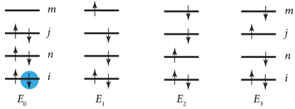
Figure 3: Ground state configuration of the neutral system and the cationic Slater determinants of interest. A hole created in the state $i$ (denoted here as a blue circle) may decay by virtue of the $1h\rightarrow 2h$-$1p$ scattering into one of the six states defined by Eqs. (62) (only three are shown).

Now we come to the most interesting non-perturbative aspect concerning the evaluation of $G_{3}^{R}$. This object is the evolution operator on a fixed subspace of three orbitals as only spin can change, see Fig. 3. To the best of our knowledge none of the established diagrammatic approximations can deal with this scenario in nonequilibrium situations. Accounting for $2h$-$1p$ correlations is, however, mandatory for a good description of the shake-up processes.

The states involved in the first two terms of Eq. (59) can be grouped into two triplets differing only by a spin flip

$$|1_{\uparrow}\rangle \equiv\hat{d}^{{\dagger}}_{m\uparrow}\hat{d}_{j\uparrow}\hat{d}_{n\uparrow}|\phi_{\rm HF}\rangle, |1_{\downarrow}\rangle \equiv\hat{d}^{{\dagger}}_{m\downarrow}\hat{d}_{j\downarrow}\hat{d}_{n\downarrow}|\phi_{\rm HF}\rangle;$$ (62a)

$$|2_{\uparrow}\rangle \equiv\hat{d}^{{\dagger}}_{m\downarrow}\hat{d}_{j\downarrow}\hat{d}_{n\uparrow}|\phi_{\rm HF}\rangle, |2_{\downarrow}\rangle \equiv\hat{d}^{{\dagger}}_{m\uparrow}\hat{d}_{j\uparrow}\hat{d}_{n\downarrow}|\phi_{\rm HF}\rangle;$$ (62b)

$$|3_{\uparrow}\rangle \equiv\hat{d}^{{\dagger}}_{m\downarrow}\hat{d}_{j\uparrow}\hat{d}_{n\downarrow}|\phi_{\rm HF}\rangle, |3_{\downarrow}\rangle \equiv\hat{d}^{{\dagger}}_{m\uparrow}\hat{d}_{j\downarrow}\hat{d}_{n\uparrow}|\phi_{\rm HF}\rangle.$$ (62c)

For any $\alpha=1,2,3$ the states $|\alpha_{\uparrow}\rangle$ have spin-projection $S_{z}=-1/2$, whereas the states $|\alpha_{\downarrow}\rangle$ have $S_{z}=1/2$. Therefore, the matrix representing the Hamiltonian $\hat{H}^{\prime}$ in the subspace $\{|\alpha_{\sigma}\rangle,\alpha=1,2,3;\sigma=\uparrow,\downarrow\}$ has a block-diagonal form with two identical $3\times 3$ blocks. Denoting by $\mathfrak{h}_{mjn;\alpha\beta}\equiv\langle\alpha_{\uparrow}|\hat{H}^{\prime}|\beta_{\uparrow}\rangle$ the matrix elements of the $3\times 3$ block one finds

$$\mathfrak{h}_{mjn}=\left(\begin{array}[]{ccc}E_{mjn}^{1}&v_{mj}^{x}&v_{mn}^{x}\\ v_{mj}^{x}&E_{mjn}^{2}&-v_{jn}^{x}\\ v_{mn}^{x}&-v_{jn}^{x}&E_{mjn}^{3}\end{array}\right),$$ (66)

with

$$E_{mjn}^{1} =\epsilon_{m}-\epsilon_{j}-\epsilon_{n}-w_{mj}-w_{mn}+w_{jn},$$ (67a)

$$E_{mjn}^{2} =\epsilon_{m}-\epsilon_{j}-\epsilon_{n}-w_{mj}-v_{mn}^{d}+v_{jn}^{d},$$ (67b)

$$E_{mjn}^{3} =\epsilon_{m}-\epsilon_{j}-\epsilon_{n}-v_{mj}^{d}-w_{mn}+v_{jn}^{d},$$ (67c)

and the direct, exchange and antisymmetrized Coulomb matrix elements read

$$v^{d}_{\mu\nu} =v_{\mu\nu\nu\mu}, v^{x}_{\mu\nu} =v_{\mu\nu\mu\nu}, w_{\mu\nu} =v^{d}_{\mu\nu}-v^{x}_{\mu\nu}.$$ (68)

We notice that using the full Hamiltonian $H$ in place of $H^{\prime}$ in the definition of $\mathfrak{h}$ would not change the result; this justifies the splitting of Coulomb integrals in Eq. (44). Our approximation for the retarded $2h$-$1p$ propagators appearing in Eq. (59) is then (omitting the subscript $mjn$)

$$\left(\begin{array}[]{ccc}{G_{3}^{R}}_{\uparrow\uparrow\uparrow}^{\uparrow\uparrow\uparrow}(t,\bar{t})&{G_{3}^{R}}_{\uparrow\uparrow\uparrow}^{\downarrow\downarrow\uparrow}(t,\bar{t})&{G_{3}^{R}}_{\downarrow\uparrow\downarrow}^{\uparrow\uparrow\uparrow}(t,\bar{t})\\[6.0pt] {G_{3}^{R}}_{\uparrow\uparrow\downarrow}^{\downarrow\downarrow\downarrow}(t,\bar{t})&{G_{3}^{R}}_{\uparrow\uparrow\downarrow}^{\uparrow\uparrow\downarrow}(t,\bar{t})&{G_{3}^{R}}_{\uparrow\uparrow\downarrow}^{\uparrow\downarrow\uparrow}(t,\bar{t})\\[6.0pt] {G_{3}^{R}}_{\downarrow\uparrow\downarrow}^{\uparrow\uparrow\uparrow}(t,\bar{t})&{G_{3}^{R}}_{\downarrow\uparrow\downarrow}^{\downarrow\downarrow\uparrow}(t,\bar{t})&{G_{3}^{R}}_{\downarrow\uparrow\downarrow}^{\downarrow\uparrow\downarrow}(t,\bar{t})\end{array}\right)=-\mathrm{i}\theta(\tau)e^{-\mathrm{i}\mathfrak{h}(\tau)}.$$ (72)

It is important to comment on the relation between the Faddeev approximation and the conventional approaches discussed in Section II. In the $GW$ approximation as well as in the $T$-matrix approximation in the $ph$ channel one of the holes is a mere spectator and only the scattering between the particle and the other hole is treated to infinite order. Similarly, in the $T$-matrix approximation in the $pp$ channel the particle is a mere spectator while the scattering between the two holes is treated nonperturbatively. It is possible to recover these approximations by retaining in the $\mathfrak{h}_{mjn}$ matrix only the direct and exchange Coulomb integrals of the considered channel. In particular, the $GW$ approximation is recovered by retaining only $v^{d}_{mn}$ and $v^{x}_{mn}$, the $T$-matrix approximation in the $ph$ channel is recovered by retaining only $v^{d}_{mj}$ and $v^{x}_{mj}$ and the $T$-matrix approximation in the $pp$ channel is recovered by retaining only $v^{d}_{nj}$ and $v^{x}_{nj}$.

III.4 Working formulas

According to Eq. (47) the collision integral can be written as

$$I^{s}_{lj}(t) =-\mathrm{i}\sum_{imn}v^{s}_{lnmi}\left(A_{imjn}+A^{\ast}_{jnim}\right),$$ (73)

where $A_{imjn}(t)\equiv\sum_{\sigma}A^{\sigma}_{imjn}(t)$. Let $\Omega^{\lambda}$ and $Y^{\lambda}$ be the eigenvalues and the eigenvectors of the $3\times 3$ Hamiltonian in Eq. (66): $\mathfrak{h}_{mjn}Y^{\lambda}_{mjn}=\Omega_{mjn}^{\lambda}Y_{mjn}^{\lambda}$. Using the spectral decomposition

$$[e^{-\mathrm{i}\mathfrak{h}\tau}]_{\alpha\beta}=\sum_{\lambda}e^{-\mathrm{i}\Omega^{\lambda}\tau}Y^{\lambda\alpha}Y^{\lambda\beta}$$ (74)

to write the $2h$-$1p$ propagator we obtain the following expression for $A_{imjn}$

$$A_{imjn}(t) =\textstyle\sum_{\lambda}\left(P_{imjn}^{\lambda}(t)+Q_{imjn}^{\lambda}(t)\right),$$ (75)

where $P_{imjn}^{\lambda}(t)$ and $Q_{imjn}^{\lambda}(t)$ are obtained from the solution of ODEs:

$$\mathrm{i}\frac{d}{dt}P_{imjn}^{\lambda}(t) =\bar{f}_{m}\Big{[}\big{(}Y_{mjn}^{\lambda 1}+Y_{mjn}^{\lambda 3}\big{)}^{2}\,\Psi_{imnj}(t)$$

$$\quad\qquad-\big{(}Y_{mjn}^{\lambda 1}+Y_{mjn}^{\lambda 3}\big{)}\big{(}Y_{mjn}^{\lambda 1}+Y_{mjn}^{\lambda 2}\big{)}\Psi_{imjn}(t)\Big{]}$$

$$\qquad+(\Omega_{mjn}^{\lambda}+\epsilon_{i})P_{imjn}^{\lambda}(t),$$ (76a)

$$\mathrm{i}\frac{d}{dt}Q_{imjn}^{\lambda}(t) =\bar{f}_{i}\Big{[}\big{(}Y_{ijn}^{\lambda 1}+Y_{ijn}^{\lambda 2}\big{)}^{2}\,\Psi_{imnj}(t)$$

$$\quad\qquad-\big{(}Y_{ijn}^{\lambda 1}+Y_{ijn}^{\lambda 3}\big{)}\big{(}Y_{ijn}^{\lambda 1}+Y_{ijn}^{\lambda 2}\big{)}\Psi_{imjn}(t)\Big{]}$$

$$\qquad+(\Omega_{ijn}^{\lambda}+\epsilon_{m})Q_{imjn}^{\lambda}(t).$$ (76b)

These equations together with Eq. (6) form a closed system of ODEs which define the Faddeev approximation within the GKBA framework. We emphasize that to obtain $\Omega^{\lambda}_{mjn}$ and $Y^{\lambda}_{mjn}$ we simply have to diagonalize $3\times 3$ matrices for every $m\in\mathcal{V}$ and for every pair $j,\,n\in\mathcal{O}$. The numerical solution of the Faddeev scheme scales linearly with the propagation time and it is therefore competitive with the conventional NEGF approaches discussed in Section II.

IV Photoinduced dynamics in glycine

As a test model for the investigation of the shake-up processes we consider the Gly I conformer of the glycine molecule in which an XUV pulse creates a hole in the inner valence states. Glycine is the simplest natural amino acid with just 15 valence molecular orbitals. Its nontrivial electronic structure Myhre et al. (2019) represents a tough test for numerical methods as discussed below. The system has been previously studied in a number of works. Kuleff et al. Kuleff et al. (2005); Kuleff and Cederbaum (2007) describe in details the periodic charge migration of a hole following its sudden creation in the $11a^{\prime}$ MO. They demonstrate that oscillations with period of about 8 fs between the $11a^{\prime}$ and $12a^{\prime}$ MOs are responsible for the major part of the dynamics. However, this is also accompanied by the excitation-deexcitation of the $4a^{\prime\prime}$ and $16a^{\prime}$ MOs, and by the promotion of an electron to the unoccupied $5a^{\prime\prime}$ MO. This picture was confirmed using the NEGF-2B method Perfetto et al. (2019). Very similar quantum beatings between $11a^{\prime}$ and $12a^{\prime}$ have been predicted in Ref. Cooper and Averbukh (2013); here the authors also propose a mechanism to experimentally detect the effect using the so-called single-photon laser-enabled Auger decay. Finally, we mention a recent DFT study tuned towards more realististic description of the initial photoinoization Ayuso et al. (2017) — the attosecond XUV pulse is explicitly taken into account leading to the broad 17 to 35 eV spectrum of excitations.

Table 2: HF energies of the five MOs participating to the reduced photoinduced dynamics of the glycine molecule. The energy level positions are indicated according to the aufbau principle with respect to highest occupied molecular orbital (HOMO) and lowest unoccupied molecular orbital (LUMO).

State	Position	HF Energy (eV)
$11a^{\prime}$	HOMO-9	$-19.15$
$12a^{\prime}$	HOMO-8	$-18.74$
$4a^{\prime\prime}$	HOMO-2	$-12.93$
$16a^{\prime}$	HOMO	$-10.86$
$5a^{\prime\prime}$	LUMO+3	$+4.79$

We consider here a reduced Hamiltonian for the Gly I conformer which takes into account only the five HF MOs involved in the dynamics of the $8$ fs charge oscillation, namely the occupied states $11a^{\prime}$, $12a^{\prime}$, $4a^{\prime\prime}$ and $16a^{\prime}$ and one unoccupied state $5a^{\prime\prime}$. The occupancies of all other valence states is frozen to the equilibrium value. The HF energies of the relevant MOs is reported in Table 2. We refer to our previous works on the electronic structure of the ground and excited states, basis representation, and femtosecond dynamics of this molecule Perfetto et al. (2019); Perfetto and Stefanucci (2018). The reduced system is ionized by coupling the MOs to a fictitious vacuum state through $\Omega(t)=E(t)\mathcal{D}$ where $\mathcal{D}$ is the dipole matrix element (chosen independent of the states) and $E(t)$ is the electric field of a weak attosecond XUV pulse causing single-photon ionizations. To better highlight correlation effects we did not consider pulse-induced transitions between different MOs, see below. We perform our calculations at the fixed geometry since the nuclear dynamics is expected to take place at longer time-scales. However, this is an important ingredient Li et al. (2015); Lara-Astiaso et al. (2017); Polyak et al. (2018) to make theory predictive in experimental energy- and time-ranges.

Figure 4: Electron occupancies of the five MO of the glycine molecule after photoionization. (a) Exact solution of the Schrödinger equation in the subspace spanned by the 5 MOs and the fictitious vacuum state (thin lines). Additionally we demonstrate that the dynamics can be resonably represented by truncating the CI expansion to $2h$-$1p$ states (thick lines). (b)-(h) GKBA simulations in different approximations.

In Fig. IV (a) we show the time-dependent change of the MO occupancies as obtained from the exact solution of the Schrödinger equation in the subspace of the 5+1 states (thin lines). Additionally we demonstrate that the dynamics can be resonably represented by taking into account only $1h$ an $2h$-$1p$ states in the configuration interaction (CI) expansion (thick lines). This implies that shake-up processes dominate the correlation-driven dynamics. During the action of the XUV pulse the occupied states loose charge mainly due to photoionization. Shake-up $1h\rightarrow 2h$-$1p$ processes initiate immediately after the pulse and are responsible for populating the virtual (unoccupied) state $5a^{\prime\prime}$. Time-dependent HF simulations clearly show the crucial role played by correlations, see panel (b). The HF Hamiltonian remains essentially the same after the pulse as only $\simeq 10^{-8}$ electrons are expelled. Since pulse-induced transitions between MOs have been neglected, the occupancies remain almost constant, and in particular the virtual state does not populate.

The considered subspace of 5 MOs well capture the 8 fs oscillation of the $11a^{\prime}$ and $12a^{\prime}$ occupancies, see again panel (a). Although this effect can be described in terms of simple $1h$ transitions between the involved MOs, the HF approximation remains inadequate. This is due to the fact that the cationic states $\hat{d}_{11a^{\prime}}|\phi_{\rm HF}\rangle$ and $\hat{d}_{12a^{\prime}}|\phi_{\rm HF}\rangle$ are not exact eigenstates of $\hat{H}$ (excited state correlations). As we shall see almost all correlated methods cure this problem; they are able to describe the bounce of charge between the $11a^{\prime}$ and $12a^{\prime}$ MOs, albeit with slightly different periods. A secondary, yet dominat, feature is the superimposed oscillation of higher frequency, with a period $\simeq 1.4$ fs. A careful inspection reveals that this faster mode can be associated to the $1h\rightarrow 2h$-$1p$ transition

$$\hat{d}_{12a^{\prime}}|\phi_{\rm HF}\rangle\to\hat{d}^{{\dagger}}_{5a^{\prime\prime}}\hat{d}_{16a^{\prime}}\hat{d}_{4a^{\prime\prime}}|\phi_{\rm HF}\rangle.$$ (83)

It turns out that this mode is much more difficult to predict, and so far it has not been accessed by any of the existing methods.

To appreciate the difficulty we have performed 2B, $GW$ and $T$-matrix simulations with and without exchange ($X$) diagrams. All these methods bring about some correlations already in the neutral ground state and, thus, it seems unavoidable to perform the adiabatic switching procedure in order to construct a stationary correlated ground state. As already discussed, however, the initial ground state of glycine is well approximated by a single Slater determinant and it is therefore accurate to start the simulation from the HF ground state. The question then arises, how the adiabatic switching can be avoided in such a way that the HF ground state is a stationary solution of the GKBA equation (6) in the absence of external fields? The answer to this question is rooted in the physics of the photoinduced dynamics. The main role of the collision integral is to initiate the shake-up process. Following the reasoning that has led us to develop the Faddeev approximation, we replace $v$ with $v^{s}$ in Eq. (9), compare with Eq. (41). Furthermore, the expansion of $\bm{\mathcal{G}}$ to lowest order in $v^{s}$ amounts to replace $v$ with $v^{s}$ also in Eq. (12). The full Coulomb tensor $\mathbfit{w}$ is instead retained in the products $\mathbfit{w}\bm{\mathit{\rho}}^{\Delta}$ and $\bm{\mathit{\rho}}^{\Delta}\mathbfit{w}$ of Eq. (18) in order to fully account for the repeated scattering between particles in the virtual $2h$-$1p$ states. It is easy to show that this adjustment is equivalent to calculate the self-energy using $v^{s}$ instead of $v$ in the external interaction lines. With this adjustment, the HF density matrix is stationary in the absence of external field for any correlated method since the $v^{s}$ Coulomb tensor has only one index in the $\mathcal{V}$-sector and $\bm{\mathit{\Psi}}$ contains the product of two $\rho^{<}=\mathrm{diag}\{1,1,1,1,0\}$ and two $\rho^{>}=\mathrm{diag}\{0,0,0,0,1\}$ — this implies that the driving term at the initial time, i. e., $\bm{\mathit{\Psi}}(0)$ vanishes.

In Fig. IV (c) we show the results of the simplest correlated approximation, i. e., the 2B approximation. Due to the lack of $h$-$h$ and $p$-$h$ scatterings, the energy of the $2h$-$1p$ state is simply given by

$$\Omega^{\rm 2B}=\epsilon_{5a^{\prime\prime}}-\epsilon_{16a^{\prime}}-\epsilon_{4a^{\prime\prime}}$$ (84)

and hence the transition energy $\Omega^{\rm 2B}+\epsilon_{12a^{\prime}}\simeq 9.8$ eV, corresponding to a period of $0.42$ fs, is severely overestimated. The situation does not improve in the $GW$ approximation, see panel (d), nor in the $T$-matrix approximation in the $pp$ channel (almost the same as in $GW$ and hence not shown). The $T$-matrix approximation in the $ph$ channel is unstable toward the formation of strongly bound electron-hole pairs; therefore we do not have results to show for $T^{ph}$. As anticipated the failure of these methods must be attributed to the absence of $2h$-$1p$ correlations. As a matter of fact they do not even take into account virtual spin-flip scatterings in the $p$-$h$ (for $GW$ and $T^{ph}$) or $p$-$p$ (for $T^{pp}$) channels since exchange diagrams are discarded.

The inclusion of exchange diagrams does not, in general, guarantee a better performance. In panel (e) we show the results of a simulation using the $T$-matrix approximation in the $ph$ channel with only exchange diagrams ($X$-only). Although $X$-only $T^{ph}$ is stable, the 1.4 fs oscillation is absent. We could perform simulations with both direct and exchange diagrams for $GW$ and $T^{pp}$. Surprisingly we found that $GW$+$X$ provides a key improvement, see panel (g), whereas exchange diagrams in $T^{pp}$ play essentially no role, see panel (f). The rational behind these outcomes should be searched in the values of the direct and exchange Coulomb integrals, i. e., $v^{d}_{\mu\nu}$ and $v^{x}_{\mu\nu}$, responsible for renormalizing the energy of the $2h$-$1p$ states, see Eqs. (66-68). It turns out that the $12a^{\prime}$ hole of spin $\sigma$ is mainly coupled (through $v^{s}$) to the $2h$-$1p$ states $16a^{\prime}_{\sigma}4a^{\prime\prime}_{\uparrow}-5a^{\prime\prime}_{\downarrow}$ and $16a^{\prime}_{\sigma}4a^{\prime\prime}_{\downarrow}-5a^{\prime\prime}_{\uparrow}$, which are in turn coupled by the anomalously large exchange integral $v^{x}_{4a^{\prime\prime},5a^{\prime\prime}}\simeq 2.3$ eV (all other exchange integrals are negligible). The energy of these two $2h$-$1p$ states is almost the same and given by

$$\Omega\simeq\Omega^{\rm 2B}+v^{d}_{4a^{\prime\prime},16a^{\prime}}-v^{d}_{5a^{\prime\prime},16a^{\prime}}-v^{d}_{4a^{\prime\prime},5a^{\prime\prime}}+v^{x}_{4a^{\prime\prime},5a^{\prime\prime}}.$$ (85)

The direct integrals are all large with $v^{d}_{4a^{\prime\prime},16a^{\prime}}\simeq v^{d}_{5a^{\prime\prime},16a^{\prime}}\simeq 6.5$ eV and $v^{d}_{4a^{\prime\prime},5a^{\prime\prime}}\simeq 10.6$ eV. Due to the cancellation between the first two direct integrals in Eq. (85) only the direct and exchange integrals with labels $4a^{\prime\prime},5a^{\prime\prime}$ are relevant in $\Omega$. These are precisely the ones taken into account by the $GW$ approximation, see discussion below Eq. (72). The inclusion of exchange, i. e., $GW$+$X$, provides a key improvement of the theory since it describes the spin-flip scattering process mediated by $v^{x}_{4a^{\prime\prime},5a^{\prime\prime}}$. We conclude that the good performance of the $GW$+$X$ approximation is a mere coincidence as it strongly relies on the particular values of the Coulomb integrals in glycine.

Time-dependent simulations in the Faddeev approximation are shown in Fig. IV (h). The results are of comparable quality to the $GW$+$X$ ones, in agreement with the discussion above. However, the Faddeev approximation does not rely on any special values of the Coulomb integrals — $2h$-$1p$ correlations are fully taken into account. This is reflected in a slightly more accurate value of the period of the superimposed oscillations, $1.33$ fs against the $1.2$ fs in $GW$+$X$ (we recall that the exact value is $1.4$ fs).

The occupations of the MOs coincide with the diagonal elements of the one-particle density matrix $\rho^{<}$. As the GKBA approach returns the full density matrix we could also investigate how accurate the off-diagonal elements are. For this purpose we have calculated the photoinduced dipole moment

$$d_{\alpha}(t)=\sum_{ij}d^{\alpha}_{ij}\rho^{<}_{ji}(t),$$ (86)

where $d^{\alpha}_{ij}$ are the dipole matrix elements along the direction $\alpha$ calculated in Ref. Perfetto et al. (2019), and then extracted the power spectrum from the Fourier transform, $\lVert d(\omega)\rVert^{2}=\frac{1}{3}\sum_{\alpha}|d_{\alpha}(\omega)|^{2}$. The outcome of exact and GKBA simulations is shown in Fig. 5. With the exception of $GW$+$X$ and Faddev all other approximations yield only four peaks; their origin is essentially the same as in HF, see top panel, although different approximations give different weights. The $GW$+$X$ represents a clear improvement over all other methods but visible discrepancies occur here too. The lowest energy and higher energy peaks are well reproduced but all other peaks are either misplaced by hundreds of meV or completely absent. In contrast the Faddeev approximation captures with high accuracy all main peaks except for the second and third low energy ones (whose energy is overstimated) and the one at energy $\simeq 6.7$ eV which is missing.

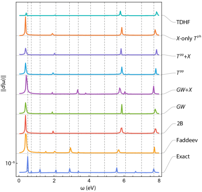
Figure 5: Power spectrum computed as the Fourier transform of the photoinduced dipole moment. The peaks associated to the $11a^{\prime}\leftrightarrow 12a^{\prime}$ quantum beating at energy 0.5 eV (period $\simeq 8$ fs) and the shake-up processes involving the electron promotion to the unoccupied $5a^{\prime\prime}$ state at energy $2.9$ eV (period $\simeq 1.4$ fs) are clearly visible. Notice, that the number of peaks is smaller than in the DFT analysis of Ayuso et al. Ayuso et al. (2017) because of the minimal model considered here.

V Conclusions

In conclusion, we have provided an accurate NEGF description and an efficient implementation scheme for the ubiquitous shake-up mechanism which accompanies the ultrafast valence-hole migration in organic molecules triggered by a weak XUV pulse. Calculations based on the unifying matrix formalism clearly demonstrate that none of the state-of-the-art NEGF methods such as second Born, $GW$ or $T$-matrix are capable to describe it. Our solution has been inspired by the three-particle Faddeev approach which treats $2h$-$1p$ scatterings non-perturbatively and it relies on an extension of the original GKBA to higher order Green’s functions. The Faddeev-NEGF scheme scales linearly in time opening prospects for the incorporation of other effects such as interaction with collective nuclear and electronic excitations and the inclusion of continuum scattering states for the accurate description of ultrafast spectroscopies of organic molecules.

Appendix A Intuition behind GKBA and its generalization to higher-order GFs

Let us start by “deriving” the generalized Kadanoff-Baym ansatz. This is just an approximation that can intuitively be derived from the following considerations for the mean-field GF. Let us express our main quantity as

$$G_{0}^{<}(t_{1},t_{2})=U(t_{1},t_{0})G_{0}^{<}(t_{0},t_{0})U(t_{0},t_{2}),$$ (87)

where $U(t_{0},t)$ is the usual time-evolution operator

$$U(t,t_{0})=T\left\{e^{-\mathrm{i}\int_{t_{0}}^{t}d\tau\,h_{\text{HF}}(\tau)}\right\}.$$ (88)

Eqs. (87,88) are understood in matrix form. Using the semi-group property of the time-evolution operator we split the time-dependence in Eq. (87)

$$G_{0}^{<}(t_{1},t_{2})=\overbrace{\theta(t_{1}-t_{2})U(t_{1},t_{2})}\overbrace{U(t_{2},t_{0})G_{0}^{<}(t_{0},t_{0})U(t_{0},t_{2})}\\ +\underbrace{U(t_{1},t_{0})G_{0}^{<}(t_{0},t_{0})U(t_{0},t_{1})}\underbrace{U(t_{1},t_{2})\theta(t_{2}-t_{1})}.$$ (91)

Recall now that Hartree-Fock retarded (advanced) GFs fulfill the equations of motion (30), and therefore they can be written in terms of the evolution operator

$$G_{0}^{\mathit{R}}(t_{1},t_{2}) =-\mathrm{i}\theta(t_{1}-t_{2})U(t_{1},t_{2}),$$ (92a)

$$G_{0}^{\mathit{A}}(t_{1},t_{2}) =+\mathrm{i}\theta(t_{2}-t_{1})U(t_{1},t_{2}),$$ (92b)

allowing us to re-write

$$G_{0}^{<}(t_{1},t_{2})=\mathrm{i}G_{0}^{\mathit{R}}(t_{1},t_{2})G_{0}^{<}(t_{2},t_{2})-\mathrm{i}G_{0}^{<}(t_{1},t_{1})G_{0}^{\mathit{A}}(t_{1},t_{2}).$$ (93)

Analogous considerations hold for the greater GF. Now the crutial step is to perform the replacements $G_{0}^{\lessgtr}(t_{1},t_{2})\rightarrow G^{\lessgtr}(t_{1},t_{2})$ and $G_{0}^{\lessgtr}(t,t)\rightarrow\mathrm{i}\rho^{\lessgtr}(t)$ because the main point of GKBA is to approximate the interacting correlators. This approximation is physically justified provided that, e. g., the quasiparticle life-time is greater than the averaged electron collision time Lipavský et al. (1986), and it leads us to the following compact form

$$G^{\lessgtr}(t_{1},t_{2}) =-G^{\mathit{R}}(t_{1},t_{2})\rho^{\lessgtr}(t_{2})+\rho^{\lessgtr}(t_{1})G^{\mathit{A}}(t_{1},t_{2}).$$ (94)

Equation (94) allows for further generalizations in the case of more complicated two-times correlators. Consider for instance a very general greater correlator

$$\mathcal{G}^{>}(1,2)=\frac{1}{\mathrm{i}^{n}}\langle\hat{\mathcal{C}}_{H}(\bar{x}_{1},t_{1})\hat{\mathcal{C}}_{H}^{\dagger}(\bar{x}_{2},t_{2})\rangle,$$ (95)

where $1\equiv(\bar{x}_{1},t_{1})$, etc., for brevity, $\hat{\mathcal{C}}_{H}(\bar{x},t)$ being a composite operator that can be expressed as a product of $n$ fermionic creation $\hat{d}^{\dagger}$ and annihilation $\hat{d}$ operators in the Heisenberg picture, and $\bar{x}$ being a collective coordinate associated with the product. Our goal is to devise a GKBA for the correlator (95) starting again with a correlator averaged over $|\phi_{\text{HF}}\rangle$. In order to simplify the discussion, we introduce a new set of fermionic operators $\hat{c}$ and $\hat{c}^{\dagger}$ as to make the Hartree-Fock state $|\phi_{\text{HF}}\rangle$ to be the vaccuum state, which we will denote for brevity as $|\phi\rangle$. Specifically we have

$$\hat{c}_{i} =\begin{cases}\hat{d}_{i}&i\in\mathcal{O}\\ \hat{d}_{i}^{\dagger}&i\in\mathcal{V}\end{cases}, \hat{c}_{i}^{\dagger} =\begin{cases}\hat{d}_{i}^{\dagger}&i\in\mathcal{V}\\ \hat{d}_{i}&i\in\mathcal{O}\end{cases},$$ (96)

where $\mathcal{O}$ denotes the set of occupied states and $\mathcal{V}$ is the set of unoccupied states. With these definitions

$$\hat{c}_{i}|\phi\rangle=0,$$ (97)

and the only operators for which the mean-field approximation to the correlator (95)

$$\mathcal{G}_{0}^{>}(\bar{x}_{1},t_{1};\bar{x}_{2},t_{2})=\frac{1}{\mathrm{i}^{n}}\langle\phi(t_{1})|\hat{\mathcal{C}}_{\bar{x}_{1}}\hat{U}(t_{1},t_{2})\hat{\mathcal{C}}_{\bar{x}_{2}}^{\dagger}|\phi(t_{2})\rangle$$ (98)

is nonvanishing are those given by the product

$$\hat{\mathcal{C}}_{\bar{x}_{1}}=\hat{c}_{\bar{x}_{11}}\hat{c}_{\bar{x}_{12}}\ldots\hat{c}_{\bar{x}_{1n}}.$$ (99)

As we mention above, this convenience is one of the reasons of introducing new fermionic operators.

In Eq. (98), we expanded the operators in the Heisenberg picture, introduced the time-evolution operator $\hat{U}(t_{1},t_{2})$, and embedded some of the time-dependence into the bra- and ket-states. Consider now the states

$$|\bar{y}\rangle=\hat{\mathcal{C}}_{\bar{y}}^{\dagger}|\phi\rangle,$$

which form a complete orthonormal system. The completeness relation

$$\frac{1}{n!}\sum_{\bar{y}}|\bar{y}\rangle\langle\bar{y}|=\mathbb{1}$$ (100)

can be used in order to factorize $\mathcal{G}_{0}^{>}$. There is a certain freedom on where it can be inserted. In order to build parallels with Eq. (93) we split Eq. (98) into two parts, proportional to $\theta(t_{1}-t_{2})$ and $\theta(t_{2}-t_{1})$, respectively. In the first part, the completness relation is inserted after $\hat{U}(t_{1},t_{2})$, and in the second part — before it. As the consequence we obtain a generalization of Eq. (93)

$$\langle\phi(t_{1})|\hat{\mathcal{C}}_{\bar{x}_{1}}\hat{U}(t_{1},t_{2})\hat{\mathcal{C}}_{\bar{x}_{2}}^{\dagger}|\phi(t_{2})\rangle\\ =\frac{1}{n!}\theta(t_{1}-t_{2})\sum_{\bar{y}}\langle\phi(t_{1})|\hat{\mathcal{C}}_{\bar{x}_{1}}\hat{U}(t_{1},t_{2})\hat{\mathcal{C}}_{\bar{y}}^{\dagger}|\phi(t_{2})\rangle\\ \times\langle\phi(t_{2})|\hat{\mathcal{C}}_{\bar{y}}\hat{\mathcal{C}}_{\bar{x}_{2}}^{\dagger}|\phi(t_{2})\rangle+\frac{1}{n!}\theta(t_{2}-t_{1})\sum_{\bar{y}}\langle\phi(t_{1})|\hat{\mathcal{C}}_{\bar{x}_{1}}\hat{\mathcal{C}}_{\bar{y}}^{\dagger}|\phi(t_{1})\rangle\\ \times\langle\phi(t_{1})|\hat{\mathcal{C}}_{\bar{y}}\hat{U}(t_{1},t_{2})\hat{\mathcal{C}}_{\bar{x}_{2}}^{\dagger}|\phi(t_{2})\rangle.$$ (105)

Let us introduce the retarded and advanced correlators

$$\mathcal{G}^{\mathit{R}}(t_{1},t_{2}) =-\frac{\mathrm{i}}{n!}\theta(t_{1}-t_{2})\big{\langle}\big{[}\hat{\mathcal{C}}_{H}(\bar{x}_{1},t_{1}),\hat{\mathcal{C}}_{H}^{\dagger}(\bar{x}_{2},t_{2})\big{]}\big{\rangle},$$ (106a)

$$\mathcal{G}^{\mathit{A}}(t_{1},t_{2}) =+\frac{\mathrm{i}}{n!}\theta(t_{2}-t_{1})\big{\langle}\big{[}\hat{\mathcal{C}}_{H}(\bar{x}_{1},t_{1}),\hat{\mathcal{C}}_{H}^{\dagger}(\bar{x}_{2},t_{2})\big{]}\big{\rangle}.$$ (106b)

This form is chosen to put them in correspondence with the $n$-body time-evolution operators, cf. Eq. (92). We furthermore notice the presence of equal-time correlators in Eq. (105) such as $\langle\phi(t_{2})|\hat{\mathcal{C}}_{\bar{y}}\hat{\mathcal{C}}_{\bar{x}_{2}}^{\dagger}|\phi(t_{2})\rangle$ and $\langle\phi(t_{1})|\hat{\mathcal{C}}_{\bar{x}_{1}}\hat{\mathcal{C}}_{\bar{y}}^{\dagger}|\phi(t_{1})\rangle$. They are analogous to the single-particle densities in Eq. (94). Performing now a transition to the correlated reference state in Eq. (105), using definitions Eqs. (95 and 106), and considering that the same arguments apply to the lesser correlator, we finally obtain

$$\mathcal{G}^{\lessgtr}(\bar{x}_{1},t_{1};\bar{x}_{2},t_{2})=\mathrm{i}\sum_{\bar{y}}\mathcal{G}^{\mathit{R}}(\bar{x}_{1},t_{1};\bar{y},t_{2})\mathcal{G}^{\lessgtr}(\bar{y},t_{2};\bar{x}_{2},t_{2})\\ -\mathrm{i}\sum_{\bar{y}}\mathcal{G}^{\lessgtr}(\bar{x}_{1},t_{1};\bar{y},t_{1})\mathcal{G}^{\mathit{A}}(\bar{y},t_{1};\bar{x}_{2},t_{2}).$$ (109)

Notice that in order to introduce the retarded and the advanced GFs in these equations we used

$$\frac{1}{n!}\theta(t_{1}-t_{2})\langle\phi|\hat{\mathcal{C}}_{H}(\bar{x}_{1},t_{1}),\hat{\mathcal{C}}_{H}^{\dagger}(\bar{x}_{2},t_{2})|\phi\rangle\\ =\frac{1}{n!}\theta(t_{1}-t_{2})\big{\langle}\phi|\big{[}\hat{\mathcal{C}}_{H}(\bar{x}_{1},t_{1}),\hat{\mathcal{C}}_{H}^{\dagger}(\bar{x}_{2},t_{2})\big{]}|\phi\big{\rangle}\\ =\mathrm{i}\mathcal{G}_{0}^{\mathit{R}}(t_{1},t_{2}),$$ (113)

where the commutator can be introduced in view of the special choice of operators (Eq. 97) that guarantee that $\hat{\mathcal{C}}_{\bar{x}_{1}}|\phi\rangle=0$.

At first glance, Eq. (109) seems to be just a trivial generalization of GKBA to many-particle scenarios. However, let us inspect the physical content of even simpler $\mathcal{G}_{0}^{\mathit{R/A}}(1,2)$ correlators. They are computed with the ordinary HF Hamiltonian, however, on the subspace of $n$-particle excitations making it similar to the multiconfiguration time-dependent Hartree-Fock approach Szalay et al. (2011). This represents a completely novel aspect of our theory. We remind the reader that in Sec. III.3 we have $n=3$, i. e., with the help of GKBA (109), we factorize the $2h$-$1p$ GF (55) into a product of two terms: the one that contains 3-particle spin correlations and the other one that contains the population dynamics, viz. Eq. (58). In order to obtain this equation we explicitly set

$$\hat{\mathcal{C}}^{\dagger}_{\bar{x}_{1}} =\hat{d}_{n\sigma_{3}}^{\dagger}\hat{d}_{j\sigma_{2}}^{\dagger}\hat{d}_{m\sigma_{1}}, \hat{\mathcal{C}}_{\bar{y}} =\hat{d}_{m\sigma^{\prime\prime}_{1}}^{\dagger}\hat{d}_{j\sigma^{\prime\prime}_{2}}^{\dagger}\hat{d}_{n\sigma^{\prime\prime}_{1}},$$ (114a)

$$\hat{\mathcal{C}}_{\bar{y}}^{\dagger} =\hat{d}_{n\sigma^{\prime\prime}_{3}}^{\dagger}\hat{d}_{j\sigma^{\prime\prime}_{2}}^{\dagger}\hat{d}_{m\sigma^{\prime\prime}_{1}}, \hat{\mathcal{C}}_{\bar{x}_{2}} =\hat{d}_{p\sigma^{\prime}_{1}}^{\dagger}\hat{d}_{r\sigma^{\prime}_{2}}\hat{d}_{s\sigma^{\prime}_{3}}.$$ (114b)

As can be seen from the definition of $\hat{\mathcal{C}}_{\bar{y}}$, we exploit the factorization of the many-body states only in the spin-sector. The equal-time $2h$-$1p$ correlators in Eq. (58) are further computed with the help of the Wick’s theorem:

$$\langle\hat{\mathcal{C}}_{\bar{y}}^{\dagger}\hat{\mathcal{C}}_{\bar{x}_{2}}\rangle=\langle\hat{d}_{n\sigma^{\prime\prime}_{3}}^{\dagger}\hat{d}_{j\sigma^{\prime\prime}_{2}}^{\dagger}\hat{d}_{m\sigma^{\prime\prime}_{1}}\hat{d}_{p\sigma^{\prime}_{1}}^{\dagger}\hat{d}_{r\sigma^{\prime}_{2}}\hat{d}_{s\sigma^{\prime}_{3}}\rangle\\ =\delta_{\sigma^{\prime\prime}_{1}\sigma^{\prime}_{1}}\rho_{mp}^{>}\left\{\delta_{\sigma^{\prime\prime}_{2}\sigma^{\prime}_{2}}\delta_{\sigma^{\prime\prime}_{3}\sigma^{\prime}_{3}}\rho_{rj}^{<}\rho_{sn}^{<}-\delta_{\sigma^{\prime\prime}_{2}\sigma^{\prime}_{3}}\delta_{\sigma^{\prime\prime}_{3}\sigma^{\prime}_{2}}\rho_{rn}^{<}\rho_{sj}^{<}\right\}.$$

Appendix B Some nonequilibrium identities

According to the Langreth rules Stefanucci and van Leeuwen (2013) we have

$$\bm{\mathit{\chi}}^{<}=\bm{\mathit{\chi}}^{0,<}+\bm{\mathit{\chi}}^{R}\cdot\mathbfit{w}\cdot\bm{\mathit{\chi}}^{0,<}+\bm{\mathit{\chi}}^{<}\cdot\mathbfit{w}\cdot\bm{\mathit{\chi}}^{0,A},$$ (117)

where quite generally the $R/A$-components are defined in terms of the $\lessgtr$-components

$$A^{R}(t,t^{\prime}) =+\theta(t-t^{\prime})\big{\{}A^{>}(t,\,t^{\prime})-A^{<}(t,\,t^{\prime})\big{\}},$$

$$A^{A}(t,t^{\prime}) =-\theta(t^{\prime}-t)\big{\{}A^{>}(t,\,t^{\prime})-A^{<}(t,\,t^{\prime})\big{\}}.$$

Regrouping the terms in Eq. (117), we obtain

$$\bm{\mathit{\chi}}^{<}\cdot(\bm{\delta}-\mathbfit{w}\cdot\bm{\mathit{\chi}}^{0,A})=(\bm{\delta}+\bm{\mathit{\chi}}^{R}\cdot\mathbfit{w})\cdot\bm{\mathit{\chi}}^{0,<}.$$ (118)

Now realize with the help of RPA

$$(\bm{\delta}-\mathbfit{v}\cdot\bm{\mathit{\chi}}^{0,A})\cdot(\bm{\delta}+\mathbfit{w}\cdot\bm{\mathit{\chi}}^{A})=\bm{\delta}\\ -\mathbfit{w}\cdot\big{[}\bm{\mathit{\chi}}^{0,A}-\bm{\mathit{\chi}}^{A}\big{]}-\mathbfit{w}\cdot\underbrace{\big{[}\bm{\mathit{\chi}}^{0,A}\cdot\mathbfit{w}\cdot\bm{\mathit{\chi}}^{A}\big{]}}_{=\big{[}\bm{\mathit{\chi}}^{A}-\bm{\mathit{\chi}}^{0,A}\big{]}}=\bm{\delta}.$$

Using this identity in Eq. 118 we obtain

$$\bm{\mathit{\chi}}^{<}=(\bm{\delta}+\bm{\mathit{\chi}}^{R}\cdot\mathbfit{w})\cdot\bm{\mathit{\chi}}^{0,<}\cdot(\bm{\delta}+\mathbfit{w}\cdot\bm{\mathit{\chi}}^{A}).$$ (121)

References

• Zhang and Averitt (2014) J. Zhang and R. Averitt, Annu. Rev. Mater. Res. 44, 19 (2014).
• Lépine et al. (2014) F. Lépine, M. Y. Ivanov,  and M. J. J. Vrakking, Nat. Photonics 8, 195 (2014).
• Kraus et al. (2018) P. M. Kraus, M. Zürch, S. K. Cushing, D. M. Neumark,  and S. R. Leone, Nature Reviews Chemistry 2, 82 (2018).
• Calegari et al. (2014) F. Calegari, D. Ayuso, A. Trabattoni, L. Belshaw, S. De Camillis, S. Anumula, F. Frassetto, L. Poletto, A. Palacios, P. Decleva, J. B. Greenwood, F. Martin,  and M. Nisoli, Science 346, 336 (2014).
• Iablonskyi et al. (2017) D. Iablonskyi, K. Ueda, K. L. Ishikawa, A. S. Kheifets, P. Carpeggiani, M. Reduzzi, H. Ahmadi, A. Comby, G. Sansone, T. Csizmadia, S. Kuehn, E. Ovcharenko, T. Mazza, M. Meyer, A. Fischer, C. Callegari, O. Plekan, P. Finetti, E. Allaria, E. Ferrari, E. Roussel, D. Gauthier, L. Giannessi,  and K. C. Prince, Phys. Rev. Lett. 119, 073203 (2017).
• Lara-Astiaso et al. (2018) M. Lara-Astiaso, M. Galli, A. Trabattoni, A. Palacios, D. Ayuso, F. Frassetto, L. Poletto, S. De Camillis, J. Greenwood, P. Decleva, I. Tavernelli, F. Calegari, M. Nisoli,  and F. Martín, J. Phys. Chem. Lett. 9, 4570 (2018).
• Hervé et al. (2020) M. Hervé, V. Despré, P. Castellanos Nash, V. Loriot, A. Boyer, A. Scognamiglio, G. Karras, R. Brédy, E. Constant, A. G. G. M. Tielens, A. I. Kuleff,  and F. Lépine, Nature Phys.  (2020).
• Kuleff et al. (2005) A. I. Kuleff, J. Breidbach,  and L. S. Cederbaum, J. Chem. Phys. 123, 044111 (2005).
• Szalay et al. (2011) P. G. Szalay, T. Müller, G. Gidofalvi, H. Lischka,  and R. Shepard, Chem. Rev. 112, 108 (2011).
• Popova-Gorelova et al. (2016) D. Popova-Gorelova, J. Küpper,  and R. Santra, Phys. Rev. A 94, 013412 (2016).
• Schüler et al. (2016) M. Schüler, Y. Pavlyukh, P. Bolognesi, L. Avaldi,  and J. Berakdar, Sci. Rep. 6, 24396 (2016).
• Usenko et al. (2016) S. Usenko, M. Schüler, A. Azima, M. Jakob, L. L. Lazzarino, Y. Pavlyukh, A. Przystawik, M. Drescher, T. Laarmann,  and J. Berakdar, New J. Phys. 18, 113055 (2016).
• Cuniberti et al. (2005) G. Cuniberti, G. Fagas,  and K. Richter, Introducing Molecular Electronics (Springer, Heidelberg, 2005).
• Cuevas and Scheer (2010) J. Cuevas and E. Scheer, Molecular Electronics: An Introduction to Theory and Experiment (World Scientific, London, 2010).
• Cardona and Ley (1978) M. Cardona and L. Ley, eds., Photoemission in Solids I General Principles (Springer, Berlin, 1978).
• Freericks et al. (2009) J. K. Freericks, H. R. Krishnamurthy,  and T. Pruschke, Phys. Rev. Lett. 102, 136401 (2009).
• Pavlyukh et al. (2015) Y. Pavlyukh, M. Schüler,  and J. Berakdar, Phys. Rev. B 91, 155116 (2015).
• Ruberti et al. (2014) M. Ruberti, V. Averbukh,  and P. Decleva, J. Chem. Phys. 141, 164126 (2014).
• Ruberti et al. (2018a) M. Ruberti, P. Decleva,  and V. Averbukh, J. Chem. Theory Comput. 14, 4991 (2018a).
• Ruberti et al. (2018b) M. Ruberti, P. Decleva,  and V. Averbukh, Phys. Chem. Chem. Phys. 20, 8311 (2018b).
• Pathak et al. (2020) H. Pathak, T. Sato,  and K. L. Ishikawa, J. Chem. Phys. 152, 124115 (2020).
• Andreussi et al. (2015) O. Andreussi, S. Knecht, C. M. Marian, J. Kongsted,  and B. Mennucci, J. Chem. Theory Comput. 11, 655 (2015).
• Nisoli et al. (2017) M. Nisoli, P. Decleva, F. Calegari, A. Palacios,  and F. Martín, Chem. Rev. 117, 10760 (2017).
• Stefanucci and van Leeuwen (2013) G. Stefanucci and R. van Leeuwen, Nonequilibrium Many-Body Theory of Quantum Systems: A Modern Introduction (Cambridge University Press, Cambridge, 2013).
• Balzer (2013) K. Balzer, Nonequilibrium green’s functions approach to inhomogeneous systems, 1st ed., Lecture notes in physics No. 867 (Springer, New York, 2013).
• Lipavský et al. (1986) P. Lipavský, V. Špička,  and B. Velický, Phys. Rev. B 34, 6933 (1986).
• Karlsson et al. (2018) D. Karlsson, R. van Leeuwen, E. Perfetto,  and G. Stefanucci, Phys. Rev. B 98, 115148 (2018).
• Hermanns et al. (2014) S. Hermanns, N. Schlünzen,  and M. Bonitz, Phys. Rev. B 90, 125111 (2014).
• Schlünzen et al. (2016) N. Schlünzen, S. Hermanns, M. Bonitz,  and C. Verdozzi, Phys. Rev. B 93, 035107 (2016).
• Bar Lev and Reichman (2014) Y. Bar Lev and D. R. Reichman, Phys. Rev. B 89, 220201(R) (2014).
• Latini et al. (2014) S. Latini, E. Perfetto, A.-M. Uimonen, R. van Leeuwen,  and G. Stefanucci, Phys. Rev. B 89, 075306 (2014).
• Cosco et al. (2020) F. Cosco, N. W. Talarico, R. Tuovinen,  and N. L. Gullo,  (2020), arXiv:2007.08901 [cond-mat.str-el] .
• Tuovinen et al. (2021) R. Tuovinen, R. van Leeuwen, E. Perfetto,  and G. Stefanucci, The Journal of Chemical Physics 154, 094104 (2021).
• Covito et al. (2018) F. Covito, E. Perfetto, A. Rubio,  and G. Stefanucci, Phys. Rev. A 97, 061401(R) (2018).
• Tuovinen et al. (2020) R. Tuovinen, D. Golež, M. Eckstein,  and M. A. Sentef, Phys. Rev. B 102, 115157 (2020).
• Pal et al. (2011) G. Pal, Y. Pavlyukh, W. Hübner,  and H. C. Schneider, Eur. Phys. J. B 79, 327 (2011).
• Perfetto et al. (2015a) E. Perfetto, A.-M. Uimonen, R. van Leeuwen,  and G. Stefanucci, Phys. Rev. A 92, 033419 (2015a).
• Perfetto et al. (2015b) E. Perfetto, D. Sangalli, A. Marini,  and G. Stefanucci, Phys. Rev. B 92, 205304 (2015b).
• Sangalli et al. (2016) D. Sangalli, S. Dal Conte, C. Manzoni, G. Cerullo,  and A. Marini, Phys. Rev. B 93, 195205 (2016).
• Pogna et al. (2016) E. A. A. Pogna, M. Marsili, D. De Fazio, S. Dal Conte, C. Manzoni, D. Sangalli, D. Yoon, A. Lombardo, A. C. Ferrari, A. Marini, G. Cerullo,  and D. Prezzi, ACS Nano 10, 1182 (2016).
• Sangalli and Marini (2015) D. Sangalli and A. Marini, Eurphys. Lett. 110, 47004 (2015).
• Perfetto et al. (2016) E. Perfetto, D. Sangalli, A. Marini,  and G. Stefanucci, Phys. Rev. B 94, 245303 (2016).
• Joost et al. (2020) J.-P. Joost, N. Schlünzen,  and M. Bonitz, Phys. Rev. B 101, 245101 (2020).
• Dahlen and van Leeuwen (2007) N. E. Dahlen and R. van Leeuwen, Phys. Rev. Lett. 98, 153004 (2007).
• Myöhänen et al. (2008) P. Myöhänen, A. Stan, G. Stefanucci,  and R. van Leeuwen, Eurphys. Lett. 84, 67001 (2008).
• Myöhänen et al. (2009) P. Myöhänen, A. Stan, G. Stefanucci,  and R. van Leeuwen, Phys. Rev. B 80, 115107 (2009).
• Puig von Friesen et al. (2010) M. Puig von Friesen, C. Verdozzi,  and C.-O. Almbladh, Phys. Rev. B 82, 155108 (2010).
• Friesen et al. (2010) M. P. v. Friesen, C. Verdozzi,  and C.-O. Almbladh, J. Phys. Conf. Ser. 220, 012016 (2010).
• Säkkinen et al. (2012) N. Säkkinen, M. Manninen,  and R. van Leeuwen, New J. Phys. 14, 013032 (2012).
• Murakami et al. (2020) Y. Murakami, M. Schüler, S. Takayoshi,  and P. Werner, Phys. Rev. B 101, 035203 (2020).
• Pavlyukh et al. (2013) Y. Pavlyukh, J. Berakdar,  and A. Rubio, Phys. Rev. B 87, 125101 (2013).
• Barbieri and Dickhoff (2001) C. Barbieri and W. H. Dickhoff, Phys. Rev. C 63, 034313 (2001).
• Faddeev (1961) L. Faddeev, Sov. Phys. JETP 12, 1014 (1961).
• Ethofer and Schuck (1969) S. Ethofer and P. Schuck, Zeitschrift für Physik 228, 264 (1969).
• Potthoff et al. (1994) M. Potthoff, J. Braun,  and G. Borstel, Z. Phys. B 95, 207 (1994).
• Barbieri et al. (2007) C. Barbieri, D. Van Neck,  and W. H. Dickhoff, Phys. Rev. A 76, 052503 (2007).
• Degroote et al. (2011) M. Degroote, D. Van Neck,  and C. Barbieri, Phys. Rev. A 83, 042517 (2011).
• Schlünzen et al. (2020) N. Schlünzen, J.-P. Joost,  and M. Bonitz, Phys. Rev. Lett. 124, 076601 (2020).
• Myhre et al. (2019) R. H. Myhre, S. Coriani,  and H. Koch, J. Phys. Chem. A 123, 9701 (2019).
• Kuleff and Cederbaum (2007) A. I. Kuleff and L. S. Cederbaum, Chem. Phys. 338, 320 (2007).
• Perfetto et al. (2019) E. Perfetto, D. Sangalli, M. Palummo, A. Marini,  and G. Stefanucci, J. Chem. Theory Comput. 15, 4526 (2019).
• Cooper and Averbukh (2013) B. Cooper and V. Averbukh, Phys. Rev. Lett. 111, 083004 (2013).
• Ayuso et al. (2017) D. Ayuso, A. Palacios, P. Decleva,  and F. Martín, Phys. Chem. Chem. Phys. 19, 19767 (2017).
• Perfetto and Stefanucci (2018) E. Perfetto and G. Stefanucci, J. Phys. Condens. Matter 30, 465901 (2018).
• Li et al. (2015) Z. Li, O. Vendrell,  and R. Santra, Phys. Rev. Lett. 115, 143002 (2015).
• Lara-Astiaso et al. (2017) M. Lara-Astiaso, A. Palacios, P. Decleva, I. Tavernelli,  and F. Martín, Chem. Phys. Lett. 683, 357 (2017).
• Polyak et al. (2018) I. Polyak, A. J. Jenkins, M. Vacher, M. E. F. Bouduban, M. J. Bearpark,  and M. A. Robb, Mol. Phys. 116, 2474 (2018).