Luminosity distance and anisotropic sky-sampling at low redshifts: a numerical relativity study

Abstract

Most cosmological data analysis today relies on the Friedmann-Lemaître-Robertson-Walker (FLRW) metric, providing the basis of the current standard cosmological model. Within this framework, interesting tensions between our increasingly precise data and theoretical predictions are coming to light. It is therefore reasonable to explore the potential for cosmological analysis outside of the exact FLRW cosmological framework. In this work we adopt the general luminosity-distance series expansion in redshift with no assumptions of homogeneity or isotropy. This framework will allow for a full model-independent analysis of near-future low-redshift cosmological surveys. We calculate the effective observational ‘Hubble’, ‘deceleration’, ‘curvature’ and ‘jerk’ parameters of the luminosity-distance series expansion in numerical relativity simulations of realistic structure formation, for observers located in different environments and with different levels of sky-coverage. With a ‘fairly-sampled’ sky, we find 0.6% and 4% cosmic variance in the ‘Hubble’ and ‘deceleration’ parameters for scales of 200 Mpc/h (corresponding to density contrasts of $\sim 0.05$ in the simulated model universe), respectively. On top of this, we find that typical observers measure maximal sky-variance of 2% and 120% in the same parameters, as compared to their analogies in the large scale FLRW model. Our work suggests the inclusion of low-redshift anisotropy in cosmological analysis could be important for drawing correct conclusions about our Universe.

I Introduction

Modern cosmology has been shaped by the success of the standard $\Lambda$ Cold Dark Matter ($\Lambda{\rm CDM}$) model in providing a consistent fit to almost all of our cosmological observations to date. At the base of this model lies the assumption that the Universe is everywhere close to a Friedmann-Lemaître-Robertson-Walker (FLRW) solution to the Einstein field equations, in such a way that the FLRW model is an accurate lowest order description of the kinematic and dynamic properties of the Universe. Among the observations consistently fit within $\Lambda{\rm CDM}$ are the temperature fluctuations in the cosmic microwave background (CMB) radiation [e.g. 1], the baryon acoustic oscillation (BAO) imprint on the galaxy distribution [e.g. 2, 3], and the distances to supernovae of type Ia [SNIa; e.g. 4, 5]. It is worth noting that the $\Lambda{\rm CDM}$ model has historically been adjusted by the addition of dark matter and dark energy in order to facilitate the explanation of data. These dark components remain unexplained in the standard model of particle physics.

Amongst the successes of the $\Lambda{\rm CDM}$ model lie some interesting tensions between our observational data and theoretical predictions. The most prominent tension in the $\Lambda{\rm CDM}$ paradigm is that of the inferred value of the Hubble parameter ($H_{0}$) from CMB observations and the direct measurement of $H_{0}$ from observations of nearby SNIa and Cepheids [6, 7, 8, 9]. While many attempts have suggested mechanisms for a partial or total relief from this tension, no one solution has yet been accepted by the community, and so the search continues [see, e.g., 10, 11, 12].

The assumption of a spatially homogeneous and isotropic FLRW model underpins analytic distance relations used to interpret most cosmological datasets. For example, the luminosity-distance redshift relation of the class of flat FLRW metrics is used for, e.g., the measurement of the Hubble constant using the local distance ladder [6, 7] and the measurement of present epoch acceleration of the Universe [13, 14]. Similarly, the FLRW geometrical assumption is at the core of conventional detections of the BAO feature in the matter distribution [15, 16] and the inference and analysis of the CMB Planck power spectrum [17, 9].

The sparsity of available cosmological data has historically made the FLRW assumption justified, since exact model symmetries were needed in order to a priori constrain the model universe enough to infer cosmological information. However, the amount of data is predicted to grow by orders of magnitude in near future surveys [e.g. 18, 19, 20]. As an example, upcoming datasets of SNIa in the 2020’s will count hundreds of thousands of supernovae and cover a large proportion of the sky – see [21] and references therein. The improved constraining power of datasets like these will allow current model assumptions to be relaxed and open the door for fully model independent analysis of cosmological data.

A number of studies have taken steps towards this goal and considered general, analytic distance measures [e.g., 22, 23, 24, 25, 26]. Specifically, Heinesen [26] presented the series-expanded luminosity distance redshift relation without making assumptions on the metric tensor of the Universe, or the field equations prescribing it. Coefficients in this series expansion contain a finite set of physically interpretable geometric degrees of freedom describing the luminosity distance in a given direction on the observer’s sky. This representation allows for fully model-independent analysis of low redshift data.

Until cosmological surveys have reached the size and sky coverage necessary for model-independent analyses, it is useful to investigate the expected impact of inhomogeneity and anisotropy within this framework in realistic numerical simulations. Numerical relativity (NR) has proven a promising avenue for cosmological simulations of nonlinear structure formation without assumptions of a global ‘background’ metric of the Universe [27, 28, 29, 30, 31].

In this work, we calculate the coefficients of the general luminosity distance series expansion in realistic cosmological simulations performed with numerical relativity. We sample structures on scales where the FLRW assumption is considered valid in most cosmological analysis. Considering observers in different local environments, and with different levels of sky coverage, allows us to assess the impact of both inhomogeneity and anisotropy on effective cosmological parameters. This work is a first step towards an upcoming in-depth analysis on the effect of survey geometry on the interpretation of observations in a locally anisotropic universe.

In Section II we review the general luminosity-distance redshift relation presented by Heinesen [26], and used in this paper. In Section III we present details of our simulations, including initial data, gauge, and post-processing analysis. We present our results in Section IV and conclude in Section V. Greek indices represent space-time indices and take values $0\ldots 3$, while Latin indices represent spatial indices and take values $1\ldots 3$, and repeated indices imply summation. We use geometric units with $G=c=1$.

II The luminosity distance in a general space-time

Here we formulate the series expansion of luminosity-distance in redshift, valid in a general universe model. We first give a brief review of the FLRW expression for the series expanded luminosity distance in Section II.1, after which we provide the analogous expression valid for a general space-time setting in Section II.2.

II.1 FLRW luminosity-distance redshift relation

Before describing the luminosity distance in a general geometry, we review the series expansion for luminosity distance in redshift under the FLRW geometrical assumption as per, e.g., Visser [32]. We consider a class of emitters and observers with worldlines that are orthogonal to the homogeneous and isotropic spatial sections of the FLRW model. In this setting, the luminosity distance, $d_{L}$, between a causally connected pair of emitters and observers is determined up to third order in redshift, $z$, by

$$d_{L,{\rm FLRW}}(z)=d_{L,{\rm FLRW}}^{(1)}z+d_{L,{\rm FLRW}}^{(2)}z^{2}+d_{L,{\rm FLRW}}^{(3)}z^{3}\,.$$ (1)

The coefficients

$$d_{L,{\rm FLRW}}^{(1)} \equiv\frac{1}{H_{o}}\,,\qquad d_{L,{\rm FLRW}}^{(2)}\equiv\frac{1-q_{o}}{2H_{o}}\,,$$ (2)

$$d_{L,{\rm FLRW}}^{(3)} \equiv\frac{-1+3q_{o}^{2}+q_{o}-j_{o}+\Omega_{ko}}{6H_{o}}\,$$

of the series expansion are given in terms of the Hubble, deceleration, jerk and curvature parameters:

$$H \equiv\frac{\dot{a}}{a}\,,\qquad\qquad q\equiv-\frac{\ddot{a}}{aH^{2}}\,,$$ (3)

$$j \equiv\frac{\dot{\ddot{a}}}{aH^{3}}\,,\qquad\Omega_{k}\equiv\frac{-k}{a^{2}H^{2}}\,,$$

where $a$ is the scale factor, an overdot represents a derivative with respect to the FLRW proper time, and $k\in\{-1,0,1\}$ determines the spatial sections as being ‘open’, ‘flat’ or ‘closed’, respectively. The subscript $o$ indicates evaluation at the point of observation. No assumptions about the field equations governing the scale factor have been imposed in formulating (1)–(3). Homogeneous and isotropic cosmological analysis which does not rely on the assumptions on field equations is sometimes referred to as ‘FLRW cosmography’ [33]. The vast majority of analyses of cosmological surveys, for instance of standardisable candles, is based on either FLRW cosmography or FLRW predictions within a particular field theory. An example of the latter is the use of general relativity with a dust source and a cosmological constant, which is used to model the late Universe in the $\Lambda{\rm CDM}$ model. As we shall see in the following section, the FLRW parameters (3), and the corresponding coefficients (2) of the luminosity distance series expansion, generalise in non-trivial ways in the presence of inhomogeneity and anisotropy, with possibly crucial implications for the interpretation of cosmological data.

II.2 General luminosity-distance redshift relation

We now consider the luminosity distance to astrophysical sources as a function of their redshift in general universe models. Specifically, we make no assumptions about the metric tensor of the space-time or the field equations prescribing it. Here we state the final result of the detailed derivations, which can be found in [26] along with a discussion of physical implications and application to the analysis of cosmological data. The luminosity distance in the vicinity of the observer is in this case given by the general expression

$$d_{L}(z)=d_{L}^{(1)}z+d_{L}^{(2)}z^{2}+d_{L}^{(3)}z^{3}+\mathcal{O}(z^{4}),$$ (4)

with coefficients

$$d_{L}^{(1)} =\frac{1}{\mathfrak{H}_{o}}\,,\qquad d_{L}^{(2)}=\frac{1-\mathfrak{Q}_{o}}{2\mathfrak{H}_{o}}\ ,$$ (5)

$$d_{L}^{(3)} =\frac{-1+3\mathfrak{Q}_{o}^{2}+\mathfrak{Q}_{o}-\mathfrak{J}_{o}+\mathfrak{R}_{o}}{6\mathfrak{H}_{o}}\,,$$

where the anisotropic parameters are defined as

$$\mathfrak{H} =-\frac{1}{E^{2}}\frac{{\rm d}E}{{\rm d}\lambda}\,,$$ (6a)

$$\mathfrak{Q} \equiv-1-\frac{1}{E}\frac{\frac{{\rm d}\mathfrak{H}}{{\rm d}\lambda}}{\mathfrak{H}^{2}}\,,$$ (6b)

$$\mathfrak{R} \equiv 1+\mathfrak{Q}-\frac{1}{2E^{2}}\frac{k^{\mu}k^{\nu}R_{\mu\nu}}{\mathfrak{H}^{2}}\,,$$ (6c)

$$\mathfrak{J} \equiv\frac{1}{E^{2}}\frac{\frac{{\rm d^{2}}\mathfrak{H}}{{\rm d}\lambda^{2}}}{\mathfrak{H}^{3}}-4\mathfrak{Q}-3\,.$$ (6d)

Here, $k^{\mu}$ is the 4-momentum of the incoming null ray, and the operator $\frac{{\rm d}}{{\rm d}\lambda}\equiv k^{\mu}\nabla_{\mu}$ is the directional derivative along the null ray with affine parameter $\lambda$. The photon energy function as measured by an observer with 4–velocity $u^{\mu}$ is $E\equiv-k^{\mu}u_{\mu}$, and $R_{\mu\nu}$ is the Ricci curvature tensor of the space-time. The set of anisotropic parameters $\{\mathfrak{H},\mathfrak{Q},\mathfrak{J},\mathfrak{R}\}$ formally enter the series expansion of $d_{L}$ in the same way as the FLRW parameters $\{H,q,j,\Omega_{k}\}$ in the expansion of $d_{L,{\rm FLRW}}$, and reduce to these parameters in the limit of exact homogeneity and isotropy. We thus denote $\{\mathfrak{H},\mathfrak{Q},\mathfrak{J},\mathfrak{R}\}$ the effective observational Hubble, deceleration, jerk and curvature parameters. Comparing the parameters (6) with their FLRW limits in (3), we see that $1/E$ plays the role of an effective ‘scale factor’ on the null cone of the observer.

The effective observational Hubble parameter $\mathfrak{H}$ can be rewritten as a multipole series in the unit vector $e^{\mu}$ defining the incoming spatial direction of the null ray (i.e. the position of the astrophysical source on the sky as seen by the observer, see Appendix B.3):

$$\mathfrak{H}(\bm{e})=\frac{1}{3}\theta-e^{\mu}a_{\mu}+e^{\mu}e^{\nu}\sigma_{\mu\nu}\,,$$ (7)

where $\theta$ is the volume expansion rate, $\sigma_{\mu\nu}$ is the volume preserving deformation (shear tensor), and $a^{\mu}$ is the 4–acceleration of the observer congruence (see Appendix B for mathematical definitions of these variables). We note that the representation of $\mathfrak{H}$ in (7) is exact, i.e., the truncation at quadrupolar order is a fundamental property of any observer congruence description and follows from the definition (6a). The multipole coefficients $\{\theta,-a_{\mu},\sigma_{\mu\nu}\}$ represent 9 scalar degrees of freedom in total. The effective deceleration parameter can also be written in exact form as an multipole series in $e^{\mu}$ as truncated at the order of the 16-pole:

$$\mathfrak{Q}(\bm{e})=-1 -\frac{1}{\mathfrak{H}^{2}(\bm{e})}\bigg{(}\overset{0}{\mathfrak{q}}+e^{\mu}\overset{1}{\mathfrak{q}}_{\mu}+e^{\mu}e^{\nu}\overset{2}{\mathfrak{q}}_{\mu\nu}$$ (8)

$$+e^{\mu}e^{\nu}e^{\rho}\overset{3}{\mathfrak{q}}_{\mu\nu\rho}+e^{\mu}e^{\nu}e^{\rho}e^{\kappa}\overset{4}{\mathfrak{q}}_{\mu\nu\rho\kappa}\bigg{)}\,,$$

with coefficients

$$\overset{0}{\mathfrak{q}}\equiv\frac{1}{3}\frac{{\rm d}\theta}{{\rm d}\tau}+\frac{1}{3}D_{\mu}a^{\mu}-\frac{2}{3}a^{\mu}a_{\mu}-\frac{2}{5}\sigma_{\mu\nu}\sigma^{\mu\nu}\,,$$

$$\overset{1}{\mathfrak{q}}_{\mu}\equiv-\frac{1}{3}D_{\mu}\theta-\frac{2}{5}D_{\nu}\sigma^{\nu}_{\;\mu}-\frac{{\rm d}a_{\mu}}{{\rm d}\tau}+a^{\nu}\omega_{\mu\nu}+\frac{9}{5}a^{\nu}\sigma_{\mu\nu}\,,$$

$$\overset{2}{\mathfrak{q}}_{\mu\nu}\equiv\frac{{\rm d}\sigma_{\mu\nu}}{{\rm d}\tau}+D_{\langle\mu}a_{\nu\rangle}+a_{\langle\mu}a_{\nu\rangle}-2\sigma_{\alpha(\mu}\omega^{\alpha}_{\;\nu)}-\frac{6}{7}\sigma_{\alpha\langle\mu}\sigma^{\alpha}_{\;\nu\rangle}\,,$$

$$\overset{3}{\mathfrak{q}}_{\mu\nu\rho}\equiv-D_{\langle\mu}\sigma_{\nu\rho\rangle}-3a_{\langle\mu}\sigma_{\nu\rho\rangle}\,,$$

$$\overset{4}{\mathfrak{q}}_{\mu\nu\rho\kappa}\equiv 2\sigma_{\langle\mu\nu}\sigma_{\rho\kappa\rangle}\,,$$ (9)

where the operator $\frac{{\rm d}}{{\rm d}\tau}\equiv u^{\mu}\nabla_{\mu}$ is the directional derivative along the 4–velocity field $u^{\mu}$ of the observer congruence, $\omega_{\mu\nu}$ is the vorticity tensor describing the rotational deformation of the observer congruence, and triangular brackets $\langle\rangle$ denote the traceless and symmetric part of the tensor in the involved indices. Similarly the effective observational curvature parameter $\mathfrak{R}(\bm{e})$ can be written as a series in $e^{\mu}$ truncated at the 16-pole level, whereas $\mathfrak{J}(\bm{e})$ is truncated at the order of the 64-pole – see Appendix B in [26] for the multipole series representations of $\mathfrak{R}(\bm{e})$ and $\mathfrak{J}(\bm{e})$. The coefficients of the multipole series expressions of $\{\mathfrak{H},\mathfrak{Q},\mathfrak{J},\mathfrak{R}\}$ are given in terms of physically interpretable kinematic variables and the curvature of space-time. Due to their truncated multipole series in $e^{\mu}$, the effective observational parameters are given in terms of a finite set of degrees of freedom. This property makes the described cosmographic representation of $d_{L}$ powerful for fully model independent analysis of cosmological data.

The multipole coefficients that determine the effective observational parameters $\{\mathfrak{H},\mathfrak{Q},\mathfrak{J},\mathfrak{R}\}$ for each direction on the sky of the observer are covariantly given in terms of the kinematic variables $\theta$, $\sigma_{\mu\nu}$, $\omega_{\mu\nu}$ and the 4–acceleration $a^{\mu}$ of the observer congruence, and their covariant derivatives, along with space-time curvature invariants. These covariant quantities are of fundamental interest in cosmology, and could be directly measured in, e.g., large datasets of supernovae using this formalism.

Inhomogeneities and anisotropies in general give rise to non-trivial corrections to the FLRW coefficients of (4): the effective observational parameters $\{\mathfrak{H},\mathfrak{Q},\mathfrak{J},\mathfrak{R}\}$ are sensitive to the local environment of the observer and the direction of the astrophysical source. Even though the parameters $\{\mathfrak{H},\mathfrak{Q},\mathfrak{J},\mathfrak{R}\}$ formally replace the FLRW parameters $\{H,q,j,\Omega_{k}\}$ in the series expansion of luminosity distance, their physical interpretation are in general not those of the FLRW space-time. For instance, $\mathfrak{Q}$ does not in general measure the physical deceleration of space, and is thus not necessarily positive in a decelerating universe model. Similarly, $\mathfrak{R}$ does not in general relate simply to the Ricci curvature of spatial sections, as $\Omega_{k}$ does in FLRW.

For the series expansion (4) to be well defined, we require the effective Hubble parameter $\mathfrak{H}$ to be differentiable and of constant sign everywhere in the domain of application of the series [see 26, for a detailed discussion on regularity requirements of the general series expansion]. For expanding universe models this translates into the requirement of positivity of $\mathfrak{H}$, which itself effectively implies the need to impose a coarse-graining scale above that of the largest collapsing regions. This ensures that the redshift function is monotonic along the null ray, such that there exists a cosmological notion of a distance-redshift relation, i.e., for distance to be a single valued function of redshift. In the context of our work, imposing a coarse-graining scale translates to employing a smoothing procedure to exclude small-scale nonlinear dynamics in our simulations, which we explain further in the next section.

III Numerical relativity simulations

In this work, we wish to remain agnostic about the existence of a global background cosmology of any kind, or the smallness of any perturbations. We therefore use numerical relativity simulations, which contain no a priori imposed physical constraints on the form of the metric tensor. This allows us to mimic as closely as possible the generality of the formalism presented in Section II.2.

We now present the general relativistic numerical simulations used in our analysis. In Section III.1 we describe the software used and the physical assumptions about the energy momentum tensor. In Section III.2 we describe the initial conditions of the simulations, chosen to be consistent with the $\Lambda$CDM matter power spectrum at early times following the recombination epoch. In Section III.3 we describe volume average properties of the simulated space-time, and the observers analysed in the subsequent analysis.

III.1 Software and physical assumptions

We use the Einstein Toolkit [ET; 34, 35], a free, open-source numerical relativity code based on the Cactus infrastructure. The ET comprises modules (“thorns”) to evolve the Einstein equations using the BSSNOK formalism [36, 37, 38] alongside the equations of general-relativistic hydrodynamics, while also providing thorns for initial data, analysis, and the handling of adaptive mesh refinement and MPI. The ET has long been used for, e.g., simulations of compact relativistic objects and the emission of gravitational waves. Recently, the ET has also been applied to simulations of inhomogeneous cosmology [39, 29, 40, 41], and has proven to be a reliable tool to study nonlinear structure formation.

In this work, we use the McLachlan thorn ML_BSSN [42] in combination with GRHydro [43, 44] to evolve cosmological initial data provided by FLRWSolver [29, see also Section III.2 below]. We refer the reader to [45] for further specifics on the simulations. However, we note here that GRHydro adopts a fluid approximation (i.e., no collisionless particles), and that our simulations contain no dark energy ($\Lambda=0$). We therefore compare our numerical calculations to the flat, matter-dominated Einstein-de Sitter (EdS) model (in line with our initial conditions, see Section III.2 below). While not explicitly enforced, we find that our simulations converge to EdS behaviour when averaged over the largest scales [see Section III.3 below and also 40, for a set of similar simulations].

Our simulations have resolution $N^{3}$ with $N=128$, and we choose physical coarse-graining scales such that individual grid cells have length $100\,h^{-1}{\rm Mpc}$ and $200\,h^{-1}{\rm Mpc}$, corresponding to total domain lengths of $12.8\,h^{-1}{\rm Gpc}$ and $25.6\,h^{-1}{\rm Gpc}$, respectively. We also perform lower-resolution simulations with $N=32$ and $64$ to show that our results are robust to changes in resolution (see Appendix C). We choose this method of coarse graining to strictly exclude small-scale nonlinearities, to ensure the positivity requirements of $\mathfrak{H}$ in the generalised series expansion are met (see discussion in Section II.2). However, in Appendix C we present simulations with a resolution-independent smoothing procedure and note that we find consistent results.

Our chosen coarse-graining scales are, respectively, comparable to and larger than the estimated ‘1%’ statistical homogeneity scale of $\sim 100h^{-1}$ Mpc measured from galaxy catalogues [46, 47]. At these scales, typical density contrasts are expected to be $\sim 1\%$ at the present epoch in the $\Lambda$CDM model. Note however that our simulations will have larger density contrasts both due to the absence of a cosmological constant and to our volume-based definition of the ‘present epoch’ in our simulations (see Section III.3). The coarse-graining scales of our analysis can nevertheless be considered conservative, as density contrasts are still within the linear regime in which the FLRW metric is usually considered safe as a lowest order description.

Figure 1: Rest-mass density, expansion rate, shear, and acceleration (panels; top left to bottom right, respectively) in a $128^{3}$ resolution simulation with a box size of $25.6h^{-1}$Gpc. Each panel shows a 2–dimensional slice through the 3–dimensional domain at $z_{\rm eff}=0$.

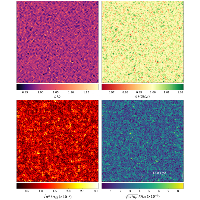
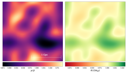
Figure 1 shows the 25.6 $h^{-1}$ Gpc, $N=128$ simulation used in this work. Panels, top left to bottom right, show the rest-mass density field relative to the global average, the expansion scalar, shear scalar $\sigma^{2}\equiv\frac{1}{2}\sigma^{\mu\nu}\sigma_{\mu\nu}$, and 4–acceleration magnitude each normalised by the global expansion, $\mathcal{H}_{\rm all}$. We show 2–dimensional slices through the midplane of the domain at effective redshift $z_{\rm eff}=0$. See Section III.3 below for definitions of $z_{\rm eff}$ and $\mathcal{H}_{\rm all}$. The expansion scalar, shear tensor, and 4–acceleration shown here are the quantities subsequently used to calculate the observational effective cosmological parameters.

III.2 Initial data and numerical gauge

FLRWSolver  is a thorn for the ET developed by Macpherson et al. [29] to generate and implement initial conditions for the linearly-perturbed, flat FLRW metric in longitudinal form, namely

$$ds^{2}=-a(\eta)^{2}(1+2\phi)d\eta^{2}+a(\eta)^{2}(1-2\phi)\delta_{ij}dx^{i}dx^{j},$$ (10)

where $\eta$ is conformal time, $a(\eta)$ is the background scale factor, and $\phi\ll 1$. The initial density fluctuations are Gaussian-random and drawn from a user-provided matter power spectrum. We use CLASS to generate the input matter power spectrum (in the longitudinal gauge) at redshift $z=1000$, with $h=0.7$ and otherwise default parameters [48]. The corresponding metric perturbation $\phi$ in (10) and the velocity field $v^{i}$ are calculated via the linearised Einstein equations in the EdS model [see 29, for details]. Sampled scales depend on the physical size of the domain and the numerical resolution: the largest mode sampled is the physical side length of the total cubic domain, and the smallest mode is $2\times$ the physical size of the grid cells. The length scales quoted in our paper in units of Mpc/h are given in terms of our choice of $h=0.7$ in CLASS. However, $h=0.7$ does not correspond to the present epoch Hubble parameter of our simulations, which is on average well approximated by the Hubble parameter of an EdS space-time (see Section III.3).

The metric is assumed to be of the form (10) on the initial hypersurface, and implicitly for the first few time steps in order to specify the extrinsic curvature $K_{ij}\propto\partial_{t}\gamma_{ij}$ on the initial slice. Throughout the simulation, however, the metric is best described in the general $3+1$ form

$$ds^{2}=-\alpha^{2}dt^{2}+\gamma_{ij}dx^{i}dx^{j},$$ (11)

where $t$ is coordinate time, $\alpha$ is the lapse function (representing the freedom of choice of coordinate time $t$), $\gamma_{ij}$ is the spatial metric, and we have forced the shift vector (describing the shift in spatial coordinates between subsequent time slices) $\beta^{i}=0$ throughout the simulation for convenience. We choose a harmonic-type evolution of the lapse function, namely $\partial_{t}\alpha=-\alpha^{2}K/3$, where $K=K^{i}_{\phantom{i}i}$ is the trace of the extrinsic curvature. In the linear regime, this translates to $\alpha^{\prime}/\alpha=a^{\prime}/a$, i.e. $\phi^{\prime}=0$ for our choice of initial metric (10), and therefore equates to choosing the pure growing mode of the linear density perturbation, $\delta$ [see 29]. Once the perturbations grow nonlinear, this interpretation of our gauge choice is no longer applicable, nor is the metric (10).

III.3 Post-processing analysis

We use a new version of the analysis code mescaline [written specifically for ET data, see 40] to calculate the terms in the series expansion (5). Mescaline adopts a uniform Cartesian grid with periodic boundary conditions, i.e. employing a torus condition on the topology of the spatial sections. Otherwise, the code is completely general, with no physical assumptions on the form of the metric or the fluid model of the energy momentum tensor.

We place 1000 observers at pseudo-randomly chosen positions within the simulation domain. The observers are co-moving with the fluid flow, such that they are moving along world lines defined by the fluid 4–velocity $u^{\mu}\equiv\frac{dx^{\mu}}{d\tau}$, where $\tau$ is the proper time. In terms of $3+1$ variables, the 4–velocity can be split into its time and space components $u^{0}=\Gamma/\alpha$, and $u^{i}=\Gamma v^{i}$, respectively (for $\beta^{i}=0$). Here, $v^{i}$ is the 3–velocity with respect to the Eulerian observer, and $\Gamma=1/\sqrt{1-v^{i}v_{i}}$ is the Lorentz factor. We note the distinction between the fluid 4–velocity $u^{\mu}$ — the physical time direction of the fluid flow in the simulation — and the normal vector $n^{\mu}$ describing the arbitrary foliation of the simulation.

(a) ‘FullSky’ sample.

(b) ‘HalfSky’ sample.

Figure 2: Example sky-maps for one observer with 300 lines of sight, representing the approximately isotropic (top) and anisotropic (bottom) sky coverage used in this work.

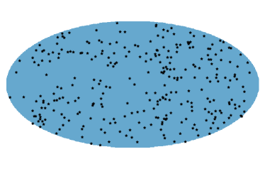
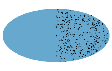
For each observer, we choose 300 pseudo-random lines of sight [similar to the number of SNe used in the local measurement of $H_{0}$ in 49]. We focus on two different examples of sky-sampling for each observer – see Appendix B.3 for details on how the sky-samplings are generated. First is the case of a ‘fairly-sampled’ sky, in which the lines of sight are chosen pseudo-randomly across the observer’s whole sky. Figure 2(a) shows an example of this distribution for one observer, which we refer to in the text and figures as the ‘FullSky’ sample. Second, we consider an ‘unfairly-sampled’ sky, in which the lines of sight are chosen pseudo-randomly across one half of the observer’s sky. Figure 2(b) shows an example of this distribution, which we refer to in the text and figures as the ‘HalfSky’ sample.

For each line of sight, $e^{\mu}$, of the sky-maps we calculate the observational effective Hubble parameter (7) using $\theta$, $\sigma_{\mu\nu}$ and $a^{\mu}$ as evaluated at the observer’s position. The remaining effective cosmological parameters (6) are subsequently built using the Ricci tensor and derivatives of $\mathfrak{H}$. See Appendix B for details of these calculations, including a consistency test using an analytic metric.

In this work we focus on calculations of the effective cosmological parameters, rather than $d_{L}(z)$ itself. However, in Appendix A we discuss the quality and convergence of the approximation of the general series expansion (4) in the context of the simulations used here.

We also use mescaline to assess the average dynamics of the simulation relative to the EdS model. This includes a calculation of the effective scale factor,

$$a_{\mathcal{D}}(t)\equiv\left(\frac{V_{\mathcal{D}}(t)}{V_{\mathcal{D},{\rm ini}}}\right)^{1/3},$$ (12)

where $V_{\mathcal{D}}(t)\equiv\int_{\mathcal{D}}\sqrt{\gamma}d^{3}X$ is the volume of a domain $\mathcal{D}$ on the spatial surfaces, $\gamma$ is the determinant of the spatial metric describing these surfaces, and $V_{\mathcal{D},{\rm ini}}\equiv V_{\mathcal{D}}(t_{\rm ini})$ is the volume on the initial slice, with $a_{\mathcal{D},{\rm ini}}=1$ for a given domain [for full details on the averaging procedure, see 40]. We also define the “effective redshift”, $z_{\rm eff}$, in order to find appropriate spatial surfaces in which to place our observers. Specifically, this is defined from (12) with $\mathcal{D}$ taken to be the total simulation domain, i.e.

$$z_{\rm eff}(t)+1\equiv\frac{a_{\mathcal{D},{\rm all}}(t_{\rm 0})}{a_{\mathcal{D},{\rm all}}(t)},$$ (13)

where $a_{\mathcal{D},{\rm all}}(t_{\rm 0})\equiv 1000$ is the value of the scale factor defining the ‘present epoch’ surface with $t=t_{\rm 0}$, which arises from our choice of $z_{\rm eff}(t_{\rm ini})+1=1000$. We also define the global average expansion rate,

$$\mathcal{H}_{\rm all} \equiv\frac{1}{3}\langle\theta\rangle_{\mathcal{D},{\rm all}}\equiv\frac{1}{3}\frac{1}{V_{\mathcal{D},{\rm all}}}\int_{\mathcal{D},{\rm all}}\theta\,\sqrt{\gamma}\,d^{3}X,$$ (14)

where $\langle\rangle_{\mathcal{D},{\rm all}}$ is the average over the entire simulation domain. In our $N=128$ simulations, the globally-averaged expansion rate at the present epoch, $\mathcal{H}_{\rm all}(z_{\rm eff}=0)$, coincides with the EdS value, $\mathcal{H}_{0,{\rm EdS}}$, to within $1\%$.

Cosmological parameters averaged over the whole domain for this simulation are $\Omega_{m}\approx 1.02$, $\Omega_{R}\approx 1\times 10^{-5}$, and $\Omega_{Q}\approx-6\times 10^{-9}$ for matter, curvature, and backreaction, respectively [see 40, for details on the calculation of these parameters]. Therefore, in terms of the cosmological parameters, the simulations converge to the EdS background model at the scale of the entire simulation domain with an accuracy of $\sim 2\%$. This deviation from the background EdS model value of $\Omega_{m}=1$ can be assigned to numerical errors (see Appendix C).

IV Results and discussion

Here we present the main findings of our analysis. In Section IV.1 we analyse anisotropies of effective cosmological parameters of the luminosity distance across the individual observer’s skies. In Section IV.2 we consider the same cosmological parameters averaged over the observer’s skies for two simple choices of survey geometries and analyse the variance between observers. In Section IV.3 we discuss the implications of our analysis for the Hubble tension present in the $\Lambda$CDM paradigm.

IV.1 Sky variance of observational effective parameters

Figure 3: Sky-maps of the effective Hubble, deceleration, curvature, and jerk parameters (top-left to bottom-right, respectively) for one observer measured in directions of the $12\times N_{\rm side}^{2}$ HEALPix pixels with $N_{\rm side}=32$. Each parameter (with the exception of the curvature) is normalised by its respective EdS value.

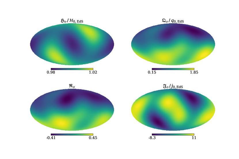
Figure 3 shows sky-maps of the observational effective Hubble, deceleration, curvature, and jerk parameters (6), relative to their respective EdS values (top left to bottom right, respectively). We show maps measured by a single observer with lines of sight in directions of the $12\times N_{\rm side}^{2}$ HEALPix [52] pixels for $N_{\rm side}=32$. We note the distinction between the resolution of the sky-maps, $N_{\rm side}=32$, and the resolution of the simulation in which we place the observers, $N=128$.

For this particular observer, we notice that the dominant form of anisotropy in the effective Hubble parameter is the quadrupole, i.e., the contribution from the shear tensor dominates the 4–acceleration term in (7). The dipole is the dominating anisotropy in the effective deceleration parameter, which can be attributed to the two first terms of $\overset{1}{\mathfrak{q}}_{\mu}$ in (II.2) involving the spatial gradient of the expansion rate and of the shear tensor, respectively. The octopole moment is also visible in the angular distribution of the effective deceleration parameter, which can be assigned to the first term of $\overset{3}{\mathfrak{q}}_{\mu\nu\rho}$ involving the spatial gradient of the shear tensor. The effective curvature parameter has similar angular distribution to the effective deceleration parameter, which is due to $\mathfrak{Q}$ entering the definition of $\mathfrak{R}$ in (6) where it dominates the anisotropic signal. The quadrupole dominates the effective jerk parameter, which can be assigned to the second spatial gradient of the expansion rate entering its quadrupole moment (see Appendix B of [26]).

Even though the maps in Figure 3 are valid for a single observer, we see common signatures between observers. Specifically, the quadrupolar anisotropy tends to dominate $\mathfrak{H}$, the dipolar and octopolar signal typically dominates $\mathfrak{Q}$ and $\mathfrak{R}$, while the quadrupole and the 16-pole typically dominate the sky distribution of $\mathfrak{J}$. This is because, in general, spatial gradients of kinematic variables dominate the anisotropic effects over the observer’s sky (with the exception of the spatial gradient of $a^{\mu}$ here, due to the small 4–acceleration amplitude of the observers). While the amplitude of the anisotropies in $\mathfrak{H}$, $\mathfrak{Q}$, $\mathfrak{R}$, and $\mathfrak{J}$ are expected to vary with smoothing scale (and the associated density contrast), the qualitative anisotropic signatures of the effective cosmological parameters found in these simulations are expected to be robust to the choice of smoothing scale and/or the inclusion of a cosmological constant, as long as the observers are well described as comoving with the matter source in a general relativistic dust description.

Figure 4: Panels (left-to-right) show the maximal sky-variance (15) for the effective Hubble, deceleration, curvature, and jerk parameters relative to their EdS counterparts. Points show $\Delta$ for 1000 observers in a simulation with a 200 $h^{-1}$ Mpc coarse-graining scale. Dashed horizontal lines show the average over all observers.

	100 $h^{-1}$ Mpc smoothing		200 $h^{-1}$ Mpc smoothing
	Obs. mean	Obs. max	Obs. mean	Obs. max
${\Delta}(\mathfrak{H}_{o}/\mathcal{H}_{0,{\rm EdS}})$	0.068	0.23	0.019	0.051
${\Delta}(\mathfrak{Q}_{o}/q_{0,{\rm EdS}})$	8.5	27	1.2	3.3
${\Delta}(\mathfrak{R}_{o})$	4.3	13	0.61	1.7
${\Delta}(\mathfrak{J}_{o}/j_{0,{\rm EdS}})$	193	675	13	37

Table 1: Anisotropy of effective cosmological parameters across typical and extreme observers’ skies. We show the mean and maximum sky-deviation $\Delta$ (15) over 1000 observers in simulations with effective smoothing lengths of 100 and 200 $h^{-1}$ Mpc.

We assess the level of anisotropy across an observer’s sky by calculating the maximal sky-deviation $\Delta$ for each parameter [similar to 53], e.g. for $\mathfrak{H}$,

$$\Delta(\mathfrak{H}_{o}/\mathcal{H}_{0,{\rm EdS}})\equiv\frac{\mathfrak{H}_{o,{\rm max}}-\mathfrak{H}_{o,{\rm min}}}{\mathcal{H}_{0,{\rm EdS}}},$$ (15)

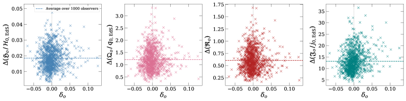
where $\mathfrak{H}_{o,{\rm max}}$ is the maximum value of $\mathfrak{H}$ across an observer’s sky, and $\mathfrak{H}_{o,{\rm min}}$ is the minimum. Figure 4 shows the maximal sky-variance $\Delta$ for the effective Hubble, deceleration, curvature, and jerk parameters, relative to their EdS counterparts (panels; left-to-right, respectively), as a function of the observers local density contrast, $\delta_{o}$. Points show $\Delta$ for 1000 observers, each with 300 ‘FullSky’ lines of sight, placed in the simulation with a 200 $h^{-1}$ Mpc coarse-graining scale. Horizontal dashed lines show the average over all observers. Here we can see the anisotropic signature as viewed by an observer is largely uncorrelated with the density contrast at the observer’s position. While the amplitude of these anisotropic effects will depend on the smoothing scale (and therefore the typical density contrasts in the simulation as a whole), observers with small $\delta_{o}$ can measure the same level of anisotropy as observers with large $|\delta_{o}|$, within a given model universe. In Table 1 we show the mean and maximum $\Delta$ across all observers shown in Figure 4, and for 1000 observers with the same lines of sight placed in the simulation with $100h^{-1}$ Mpc smoothing length.

Analyses of the FLRW Hubble and/or deceleration parameters in SNe [54, 55, 56, 53, 57] and galaxy data [58, 59] come to diverse conclusions regarding the level of anisotropy in such data. These studies employ different phenomenological anisotropic modelling and consider different survey geometries. The truncation of the cosmographic representation and the relevant choice of smoothing scale will vary according to the redshift coverage of the survey in question (see Appendix A for discussions on the level of approximation of the luminosity distance Taylor series expansion), and we thus expect different survey geometries to yield different empirical results on anisotropy in effective cosmological parameters. We should note that these works adopt FLRW cosmographic expansions – as truncated according to FLRW model arguments – in their search for anisotropy, which makes a direct comparison to our analysis difficult.

Typical observers in our analysis have dipolar contribution to the deceleration parameter dominating over the monopolar contribution. This signature has interestingly been seen for us as observers in [57] where the dipolar contribution to the deceleration parameter was found to dominate over the monopole out to scales of $z\sim 0.1$ in an empirical examination of SNe data.

IV.2 Sky averages of observational effective parameters

Figure 5: Effective cosmological parameters (6) relative to their EdS counterparts (panels) calculated in an inhomogeneous numerical relativity simulation. Points show individual observers, with local density $\delta_{o}$, averaged over 300 randomly chosen lines of sight across their whole sky (see Figure 2(a)). Dashed lines of the same colour show averages over all points on each panel, and dot-dashed lines show $\Lambda{\rm CDM}$  parameters relative to EdS.

Figure 6: Effective cosmological parameters (6) relative to their EdS counterparts (panels) calculated in an inhomogeneous numerical relativity simulation. Points show individual observers, with local density $\delta_{o}$, averaged over 300 randomly chosen lines of sight across half of their whole sky (see Figure 2(b)). Dashed lines of the same colour show averages over all points on each panel, and dot-dashed lines show $\Lambda{\rm CDM}$  parameters relative to EdS.

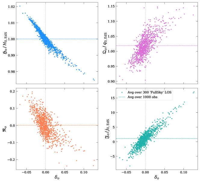
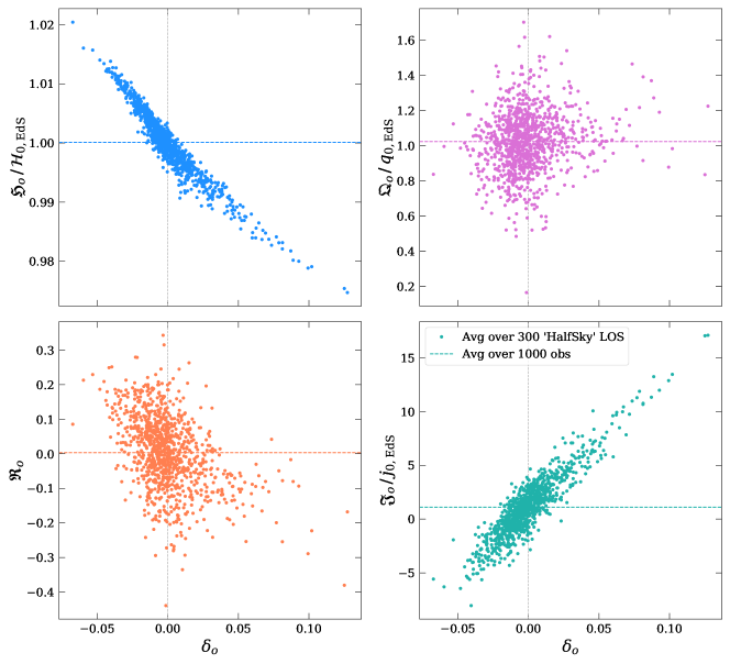
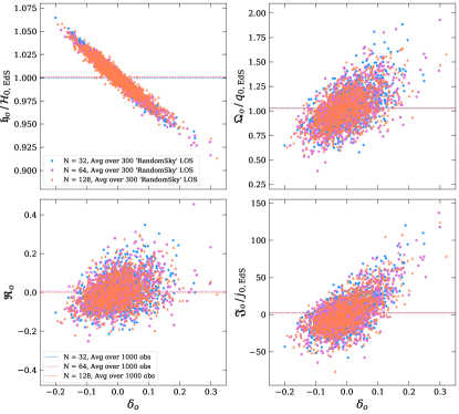
Figures 5 and 6 show our calculations of sky averages of the effective cosmological parameters in the simulation shown in Figure 1 (200 $h^{-1}$ Mpc smoothing). Panels, top-left to bottom-right, show the effective observational Hubble, deceleration, curvature, and jerk parameters, respectively, each relative to their respective EdS parameter counterpart in (2). Points represent the effective parameters of individual observers as averaged over 300 lines of sight distributed according to a ‘FullSky’ sample (Figure 5) and a ‘HalfSky’ sample (Figure 6). See Figure 2 for examples of these sky samplings. Horizontal axes indicate the local density contrast $\delta_{o}\equiv\rho_{o}/\langle\rho\rangle_{\mathcal{D},{\rm all}}-1$ at each observer’s position. Dashed lines of the same colour as the points in each panel show the average over all 1000 observers (i.e., the average over all points), and dot-dashed black lines show the $\Lambda{\rm CDM}$ value of the corresponding parameter (those panels without these lines are those where the $\Lambda{\rm CDM}$ reference lies outside the limits of the plot).

$\sigma({\rm sky\,avgs})$	100 $h^{-1}$ Mpc smoothing		200 $h^{-1}$ Mpc smoothing
	‘FullSky’	‘HalfSky’	‘FullSky’	‘HalfSky’
$\sigma(\mathfrak{H}_{o}/\mathcal{H}_{0,{\rm EdS}})$	0.022	0.021	0.0057	0.0057
$\sigma(\mathfrak{Q}_{o}/q_{0,{\rm EdS}})$	0.19	1.2	0.038	0.17
$\sigma(\mathfrak{R}_{o})$	0.22	0.64	0.064	0.11
$\sigma(\mathfrak{J}_{o}/j_{0,{\rm EdS}})$	43	43	2.9	2.9

Table 2: Cosmic variance of observational effective cosmological parameters (6). We show standard deviations of the distribution of sky averages — for the ‘FullSky’ and ‘HalfSky’ distributions (see Figure 2) — for 1000 observers placed in simulations with effective smoothing lengths of 100 and 200 $h^{-1}$ Mpc.

In Table 2 we show the standard deviation for each distribution in Figures 5 and 6, as well as the same calculation in a simulation with a smaller coarse-graining scale of 100 $h^{-1}$ Mpc. The variances in the effective Hubble and jerk parameters show no appreciable change moving from the ‘FullSky’ to the ‘HalfSky’ sampling, for both smoothing scales. However, we see drastic change in the effective deceleration and curvature parameters. For the deceleration, $\mathfrak{Q}_{o}$, we see an $\sim 6.3\times$ ($\sim 4.5\times$) increase in standard deviation when sampling only half of each observer’s sky with a smoothing length of 100 (200) $h^{-1}$Mpc. The curvature parameter, $\mathfrak{R}_{o}$, shows a $\sim 2.9\times$ ($\sim 1.7\times$) increase in standard deviation in the same case. These changes in variance can be visualised using the example observer sky map in Figure 2. Consider averaging over our ‘HalfSky’ distribution for the effective Hubble and jerk parameters for this observer. Since the quadrupolar mode is dominating the signal, cutting the sky in half (in the way we have done) should have minimal effect on the measured variance in those parameters. Considering either the effective deceleration or curvature parameter, cutting the sky in half should affect the measured variance by this observer due to the dominance of the dipole.

Comparing Figures 5 and 6 shows us that an observer can infer drastically different effective cosmological parameters when not fairly sampling their whole sky. However, we emphasise that the variances presented here are valid only for our specific ‘HalfSky’ distribution, and averages across different anisotropic sky-samplings will produce different variances. It is also important to note that the corrections to the EdS model expectation of the cosmological parameters decrease with an increase in smoothing scale. The choice of a physically relevant smoothing scale is therefore important and depends on the redshift span of the survey in question. For instance, to consistently model a survey with minimum redshifts of $0.02$, corresponding to distances from the observer of $\sim 100$ $h^{-1}$ Mpc, we should not employ larger smoothing scales than $\sim 100$ $h^{-1}$ Mpc in our modelling. To ensure a consistent fit for the entire survey, the highest-redshift data should also be well approximated by the same cosmographic representation as the lowest-redshift data. In Appendix A, we show that a consistent cosmographic representation of luminosity distance considering redshifts $\sim 0.02$ out to $z\sim 1$ (and even $z\sim 0.15$) is difficult in the presence of anisotropy. However, we stress that the interpretation of the observational effective cosmological parameters presented here remains valid as long as $z<1$ even if the truncated third order expansion (4) breaks down as an accurate approximation of the exact function $z\mapsto d_{L}(z)$.

We intend to investigate these issues relating to smoothing scale, and the impact of survey geometry on cosmological inference, in future work.

IV.3 Implications for a measurement on the local Hubble constant

The sky averages shown in Figure 5 are representative of the monopole (isotropic) contribution to the effective parameters. Focusing on the effective Hubble parameter (top left panel, with variances in the top row of Table 2), we find isotropic variances of 0.5% (2%) with respect to the EdS value, with maximum variances of up to 2% (6%) on scales 200 (100) $h^{-1}$ Mpc. This represents the variance in the $\theta/3$ term in (7) when moving between different positions in the simulation. Figure 5 shows a clear and physically expected correlation between values of $\theta/3$ and the local density. For similar local density contrasts $\delta$ (and/or similar smoothing scales), we find the above variance is in broad agreement with cosmic variance in the FLRW local Hubble parameter studied analytically [60, 61] and in the context of Newtonian N-body [62, 63, 64] and NR simulations [45].

In addition to this variance based on inhomogeneity (observer position), we have an anisotropic contribution to the effective Hubble parameter $\mathfrak{H}$, which will vary across each observer’s sky. In this work, the anisotropy in $\mathfrak{H}$ comes primarily from the shear tensor, i.e. the third term in (7). The top row of Table 1 shows that typical observers measure $6.8\%$ ($1.9\%$) maximum deviation in $\mathfrak{H}$ across their sky for 100 (200) $h^{-1}$ Mpc coarse-graining scales. We also find that 11% of the observers measure >10% maximal deviation $\Delta$ in $\mathfrak{H}$ across their sky in the simulation with 100 $h^{-1}$ Mpc coarse-graining scale.

However, this is not necessarily indicative of how many observers will measure a sky-average of $\mathfrak{H}$ to be $\sim 10\%$ larger than the global mean [as found in, e.g., 7, for the local FLRW Hubble parameter]. The specific survey geometry will affect the number of observers we find to measure a higher local $\mathfrak{H}$. We intend to investigate the role of anisotropy in context of the Hubble tension in detail in future work.

V Conclusions

The general luminosity-distance redshift relation presented by Heinesen [26] offers the potential to completely relax the assumptions of exact homogeneity and isotropy at the base of most cosmological data analysis. Additional degrees of freedom introduced — because of the lack of assumptions made — means that more cosmological data is required in order to use this framework to convey fully model-independent data analysis.

We have calculated the observational effective cosmological parameters (6) in simulations with realistic initial conditions evolved with numerical relativity. Our simulations therefore share the qualities of the general formalism in that they contain no assumptions of a global background metric. We have used conservative coarse-graining scales to study the variance of these parameters on scales where the simulated model universe is well within the linear regime of density contrasts. We find that effective cosmological parameters can be significantly anisotropic across the observers’ skies (see Figure 2 for an example), with corrections to the relevant FLRW parameters even in the monopole limit of a fairly sampled sky.

Considering a cosmographic representation of luminosity distance with a 200 $h^{-1}$ Mpc smoothing scale, our main conclusions are:

• The effective Hubble parameter has $0.5\%$ cosmic variance between observers relative to the EdS value in the monopole limit, i.e. a fairly-sampled sky. We find that $\sim$7% of observers measure a Hubble parameter $>$3% different from the EdS value in this limit (see Table 2 and Figure 5).

• Maximal quadrupolar anisotropies in the effective Hubble parameter across an observers sky are typically 2%, and can be as large as 5% (see Table 1).

• A uniform sky-average of the effective deceleration parameter has standard deviation of 4% between observers relative to the EdS value (see Table 2).

• The dipolar signal of the effective deceleration parameter dominates the monopolar contribution for typical observers, with the mean observer seeing a 120% deviation between highest and lowest value on their sky (see Table 1).

• A half-sampled sky can bias some observers measurements such that they measure acceleration without any actual accelerated expansion of space.

As a final note, since our study is concerned only with large scales — and therefore small density contrasts — we expect our results to be well-approximated in the weak-field limit of general relativity. Therefore, a re-analysis of the general observational effective parameters in the context of weak-field N-body cosmological simulations [i.e. gevolution, see 65, 66, 67], or simulations using the fully-constrained formulation of GR [i.e. GRAMSES, see 68, 69] may produce similar results. This could also be investigated in the context of constrained cosmological simulations reconstructing the environment surrounding the local group, as done in, e.g., [70].

Our main conclusions suggest that the consideration of local anisotropies could be important for cosmological analysis. The anisotropic cosmographic representation of luminosity distance [26] used in this work gives us a framework to interpret near-future large cosmological surveys in a completely model-independent way. This may be necessary to ensure we draw correct conclusions about the cosmic expansion and acceleration of the Universe.

Appendix A Convergence of the series expansion

We now examine the convergence and quality of the approximation of the Taylor series (5). For investigating these properties of the series expansion in detail, we must ideally employ ray tracing algorithms for comparison to the exact expression. Employing ray tracing is indeed our goal for future work, but for the purpose of analysing the results of this paper, we shall rely on crude order of magnitude arguments. We can note that the FLRW series expansion of luminosity distance in redshift is convergent for redshifts of $z<1$, after which the series in general breaks down [71]. Following the arguments in Section 4.1 of [71], we might define $\mathfrak{H}_{o}$, $\mathfrak{Q}_{o}$ and $\mathfrak{J}_{o}$ through the series expansion of $1/(1+z)\equiv\frac{E_{o}}{E}$ around the point of observation in the following way:

$$\frac{1}{1+z} =1+\mathfrak{H}_{o}E_{o}\Delta\lambda-\frac{1}{2}(\mathfrak{Q}_{o}+1)\mathfrak{H}^{2}_{o}E^{2}_{o}\Delta\lambda^{2}$$ (16)

$$+\frac{1}{6}(\mathfrak{J}_{o}+4\mathfrak{Q}_{o}+3)\mathfrak{H}^{3}_{o}E^{3}_{o}\Delta\lambda^{3}+\mathcal{O}(\Delta\lambda^{4})\,,$$

where $\Delta\lambda\equiv\lambda-\lambda_{o}$, and where $\lambda$ is an affine parameter of the null ray. We see that the series expansion (16) has a pole at $z=-1$ for each null ray, and the radius of convergence must thus be at most $|z|=1$, such that the series also fails to converge at $z>1$. Consequently, when inverting this series, to obtain $\Delta\lambda$ as a function of $z$, we should not expect this series to be convergent for $z>1$ either. Thus, we do not expect (5) to converge beyond $z>1$, but have no reason to believe that it will diverge at smaller scales either, if the regularity requirements discussed in [26] are satisfied in addition (which is the case in our analysis).

The quality of the approximation of the Taylor series (5) truncated at third order can however be very poor at redshifts approaching 1, and we expect this to be the case in the present simulation setup for most observers for the following reason. Spatial gradients of order ($n-1$) of kinematic fluid variables enter in the $n$’th coefficient $d_{L}^{(n)}$ in (5) – see for instance $\overset{1}{\mathfrak{q}}_{\mu}$ and $\overset{3}{\mathfrak{q}}_{\mu\nu\rho}$ in (II.2) which contain the first order spatial gradient of the expansion rate and of the shear tensor, respectively. We can make the following order of magnitude estimate of the $n$’th term $d_{L}^{(n)}z^{n}$ in the Taylor series (5) in terms of the smoothing scale $\Delta X$ of the simulation and $\mathfrak{H}_{o}$

$$\left|\frac{d_{L}^{(n)}z^{n}}{d_{L}^{(1)}z}\right|\lesssim\frac{1}{n!}\frac{z^{n-1}}{(\Delta X\mathfrak{H}_{o})^{n-1}}{\rm sup}\left(\left|\frac{\Delta\mathfrak{H}_{o}}{\mathfrak{H}_{o}}\right|\right)\,,\quad n\geq 2$$ (17)

where $\Delta\mathfrak{H}_{o}$ is the increase of $\mathfrak{H}_{o}$ to a neighbouring grid cell of the observer, and ${\rm sup}$ denotes the supremum (here corresponding to the maximum value) over all grid cells. Substituting the EdS value of the Hubble constant $\mathcal{H}_{\rm 0,EdS}\approx 45$ km/s/Mpc for $\mathfrak{H}_{o}$, gives $1/(\Delta X\mathfrak{H}_{o})\sim 50\times 100\,h^{-1}{\rm Mpc}/\Delta X$.

Let us first consider $\Delta X=100\,h^{-1}$Mpc for which we use the estimate ${\rm sup}\left(\left|\Delta\mathfrak{H}_{o}/\mathfrak{H}_{o}\right|\right)\sim 0.1$ which corresponds to $\sim 3\times\sigma(\mathfrak{H}/\mathcal{H}_{0,{\rm EdS}})$ given in Table 2. With these values we have $\left|d_{L}^{(m)}/d_{L}^{(1)}\times z^{m-1}\right|\lesssim 0.01$ for all $m\geq 4$ when $z\lesssim 0.03$. The coarse-graining scale of $\Delta X=100\,h^{-1}$Mpc itself corresponds to $z\sim 0.02$. We therefore expect the Taylor series expansion as truncated at third order to approximate the exact luminosity distance to within one percent for $0.02\lesssim z\lesssim 0.03$.

Let us next consider $\Delta X=200\,h^{-1}$Mpc. We have a similar order of magnitude estimate of ${\rm sup}\left(\left|\Delta\mathfrak{H}_{o}/\mathfrak{H}_{o}\right|\right)\sim 0.1$ for these scales. In this case we satisfy $\left|d_{L}^{(m)}/d_{L}^{(1)}\times z^{m-1}\right|\lesssim 0.01$ for all $m\geq 4$ when $z\lesssim 0.06$. The coarse-graining scale of $\Delta X=200\,h^{-1}$Mpc corresponds to $z\sim 0.04$, and we expect the truncated Taylor series (5) to provide an approximate luminosity distance to within one percent for $0.04\lesssim z\lesssim 0.06$.

If we for instance wanted to approximate scales out to $z=0.15$, the minimum integer, $m_{\rm max}$, satisfying $\left|d_{L}^{(m)}/d_{L}^{(1)}\times z^{m-1}\right|\lesssim 0.01$ for all $m\geq m_{\rm max}$ is $m_{\rm max}=9$ (18) for a smoothing scale $\Delta X=200$ (100) $h^{-1}$Mpc Thus, in order to obtain a consistent cosmography valid from scales of $200\,h^{-1}$Mpc ($z\approx 0.04$) and out to $z=0.15$, with error terms of $\lesssim 1\%$, we expect to have to include terms up to $8^{\rm th}$ order in the series expansion of $d_{L}$.

We note that as long as we remain within the radius of convergence of the Taylor series expansion of $d_{L}$ in $z$, the interpretation of the parameters $\{\mathfrak{H},\mathfrak{Q},\mathfrak{J},\mathfrak{R}\}$ as effective observational Hubble, deceleration, curvature and jerk parameters is preserved. While the radius of convergence must be examined in detail with ray tracing codes, we a priori have no reason to expect failure of convergence before $|z|=1$ is reached, as per the discussion above.

It might seem surprising that the cosmographic representation of luminosity distance (5) is not perturbatively close the analogous expression for the background EdS model, since the smoothing scales employed in the present analysis are such that density contrasts are within the linear regime. However, the higher order effective cosmological parameters $\{\mathfrak{Q},\mathfrak{J},\mathfrak{R}\}$ can be non-linear even if the density field is in the linear regime on account of the spatial gradients entering the various multipole coefficients (see for instance the multipole expansion of $\mathfrak{Q}$ in (II.2)). Since our analysis is in the linear density contrast regime, we expect our results to be repeatable in Newtonian simulations.

We could of course have employed even larger coarse-graining scales, for a well behaved Taylor series out to larger $z$. However, this would come at the price of a poorly approximated distance-redshift relation at small scales. Our analysis suggests that a well-defined, collective cosmographic representation of distance-redshift data from scales $\sim 100h^{-1}$ Mpc and up to redshifts of $z\sim 1$ is challenging.

Appendix B Mescaline calculations

Mescaline is a post-processing analysis code for Einstein Toolkit data [40]. Here we use an extended version of mescaline  to calculate each of the terms in the series expansion (4) for a chosen number of observers (randomly placed in the simulation domain) each with a chosen number of lines of sight $e^{\mu}$ (either randomly chosen across the whole sky or within a restricted region).

Mescaline contains no physical assumptions on the form of the metric, fluid, or extrinsic curvature. Mescaline reads data output from the Einstein Toolkit, in Hierarchical Data Format 5 (HDF5), and is therefore written in terms of $3+1$ variables associated with the coordinate representation (11) of the general metric. Specifically, it reads the spatial metric $\gamma_{ij}$, the extrinsic curvature $K_{ij}\propto\partial_{t}\gamma_{ij}$, the lapse function $\alpha$, the rest-mass density $\rho$, and the 3-velocity $v^{i}$ of the fluid (with respect to the Eulerian observer comoving with the foliation defined by $t$) for the whole spatial grid for all relevant time steps. The code enforces a gauge condition with shift vector $\beta^{i}=0$ (but for any $\alpha$ and $\partial_{t}\alpha$), and a uniform Cartesian grid with periodic boundary conditions (equivalent to applying a torus condition on the topology of the spatial sections)All derivatives (in time and space) are taken using fourth-order finite differences.

In this appendix we outline the key calculations required for each of the terms (5). To calculate the effective Hubble parameter, $\mathfrak{H}$, we need the volume expansion rate, shear tensor and 4-acceleration, respectively defined as

$$\theta \equiv\nabla_{\mu}u^{\mu},$$ (18)

$$\sigma_{\mu\nu} \equiv b^{\alpha}_{\mu}\,b^{\beta}_{\nu}\,\nabla_{(\alpha}u_{\beta)}-\frac{1}{3}\theta\,b_{\mu\nu},$$

$$a^{\mu} \equiv u^{\nu}\nabla_{\nu}u^{\mu}.$$

Here, $u^{\mu}$ is the 4-velocity of the fluid (which we choose to coincide with the 4-velocity of the observers), round brackets imply symmetrisation over indices, $\nabla_{\mu}$ is the Levi-Civita connection (covariant derivative) associated with $g_{\mu\nu}$, and $b_{\mu\nu}\equiv g_{\mu\nu}+u_{\mu}u_{\nu}$ is the spatial projection tensor in the frame of the fluid flow.

B.1 Derivatives along the null ray

To calculate the effective cosmological parameters (6), we need the first and second derivatives of $\mathfrak{H}$ along the null ray, i.e., the derivatives with respect to affine parameter $\lambda$. In terms of $3+1$ variables, these are

$$\frac{{\rm d}\mathfrak{H}}{{\rm d}\lambda} =k^{\mu}\nabla_{\mu}\mathfrak{H},$$ (19)

$$=k^{0}\partial_{t}\mathfrak{H}+k^{i}\partial_{i}\mathfrak{H},$$ (20)

and therefore

$$\frac{{\rm d}^{2}\mathfrak{H}}{{\rm d}\lambda^{2}}= (k^{0})^{2}\partial^{2}_{t}\mathfrak{H}+2k^{0}k^{i}\partial_{t}\partial_{i}\mathfrak{H}+k^{i}k^{j}\partial_{i}\partial_{j}\mathfrak{H}$$ (21)

$$-\frac{\partial_{t}\mathfrak{H}}{\alpha}\left[(k^{0})^{2}\partial_{t}\alpha+2k^{0}k^{i}\partial_{i}\alpha-k^{i}k^{j}K_{ij}\right]$$

$$-\partial_{i}\mathfrak{H}\left[(k^{0})^{2}\alpha\gamma^{ij}\partial_{j}\alpha-2\alpha k^{0}k^{j}K^{i}_{j}+k^{j}k^{k}\Gamma^{i}_{jk}\right],$$

where $t$ is the coordinate time of the simulation, $\partial_{\mu}\equiv\partial/\partial x^{\mu}$, and $\Gamma^{i}_{jk}$ are the Christoffel symbols associated with the spatial metric $\gamma_{ij}$. In deriving (21), we have used the time components of the 4-Christoffel symbols associated with the metric $g_{\mu\nu}$, namely,

$${}^{(4)}\Gamma^{0}_{00} =\frac{1}{\alpha}\partial_{t}\alpha,\quad\quad{}^{(4)}\Gamma^{i}_{j0}=-\alpha K^{i}_{j},$$ (22a)

$${}^{(4)}\Gamma^{i}_{00} =\alpha\gamma^{ij}\partial_{j}\alpha,\quad{}^{(4)}\Gamma^{0}_{0i}=\frac{1}{\alpha}\partial_{i}\alpha,$$ (22b)

$${}^{(4)}\Gamma^{0}_{ij} =-\frac{1}{\alpha}K_{ij},$$ (22c)

and we note that for $\beta^{i}=0$ we have ${}^{(4)}\Gamma^{i}_{jk}=\Gamma^{i}_{jk}$.

B.2 4-Ricci tensor

For the effective curvature parameter, $\mathfrak{R}$, we need the components of the (symmetric) 4-Ricci tensor, $R_{\mu\nu}$. In terms of $3+1$ variables, the time-time component is

$$R_{00}=\alpha\partial_{j}(\alpha) \partial_{i}\gamma^{ij}+\alpha\gamma^{ij}\partial_{i}\partial_{j}\alpha+\alpha\partial_{t}K$$ (23)

$$+\alpha\Gamma^{i}_{ji}\gamma^{jk}\partial_{k}\alpha-\alpha^{2}K_{ij}K^{ij},$$

the time-space components are

$$R_{0i} =\alpha\partial_{i}K-\alpha\partial_{j}K^{j}_{i}-\alpha\Gamma^{j}_{kj}K^{k}_{i}+\alpha\Gamma^{j}_{ki}K^{k}_{j},$$ (24)

and the spatial components are

$$R_{ij}={}^{(3)}\mathcal{R}_{ij} +KK_{ij}-2K^{l}_{j}K_{il}$$ (25)

$$-\frac{1}{\alpha}\left(\partial_{t}K_{ij}+\partial_{i}\partial_{j}\alpha-\partial_{k}(\alpha)\Gamma^{k}_{ij}\right),$$

where ${}^{(3)}\mathcal{R}_{ij}$ is the Ricci tensor of the spatial surfaces, and $K=K^{i}_{\phantom{i}i}$.

B.3 Direction vector

The photon 4–momentum, $k^{\mu}$, of an incoming null ray can always be decomposed based on the observer 4–velocity, $u^{\mu}$, in the following way:

$$k^{\mu}=E(u^{\mu}-e^{\mu}),$$ (26)

where $E\equiv-k^{\mu}u_{\mu}$ is the observed energy of the photon, and $e^{\mu}$ denotes the spatial direction of observation satisfying the orthonormal requirement

$$g_{\mu\nu}e^{\mu}e^{\nu}=1,\quad e^{\mu}u_{\mu}=0.$$ (27)

The direction vector $e^{\mu}$ specifies the photon 4–momentum uniquely up to the normalisation $E$. We generate sky-maps of lines of sight of the observers in our analysis (see Figure 2 for example sky-maps) by setting

$$e^{i}=D\,m^{i},$$ (28)

where $m^{i}$ are pseudo-random numbers. To generate the so-called ‘FullSky’ distribution (see Figure 2(a)) for each observer, each component of $m^{i}$ is drawn from a uniform distribution over the range $[-1,1)$. To generate the ‘HalfSky’ distribution (see Figure 2(b)), two of the components of $m^{i}$ are drawn from a uniform distribution over the interval $[-1,1)$, while the remaining component is constrained to the range $[0,1)$. The normalisation factor $D$ and the time-component $e^{0}$ are determined from the constraints (27), which give

$$e^{0} =\frac{\pm m^{i}u_{i}}{\sqrt{u_{0}^{2}\gamma_{ij}m^{i}m^{j}-\alpha^{2}m^{i}m^{j}u_{i}u_{j}}},$$ (29)

$$D =\frac{\mp u_{0}}{\sqrt{u_{0}^{2}\gamma_{ij}m^{i}m^{j}-\alpha^{2}m^{i}m^{j}u_{i}u_{j}}}.$$ (30)

B.4 Analytic test

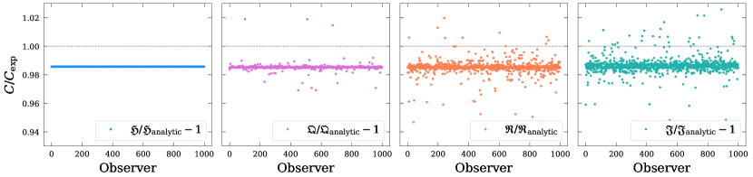
The calculations of $\mathfrak{H}$ and its derivatives (19) and (21), as presented above are new in mescaline. We must therefore test these calculations against a suitable analytic solution to ensure they are accurate, with errors converging at the expected rate.

Rather than passing in simulation output HDF5 data, we use the mescaline  test suite to pass in an analytic form of the metric, extrinsic curvature, and matter content. This analytic metric is then passed through the regular, general mescaline  routines which produce output as usual. We can then directly compare the output effective parameters with the analytic solutions to follow.

This test is not intended to place error bars on the results presented in the main text (however, see Appendix C). Here, we are isolating the mescaline calculations from the NR simulations, and not only ensuring that we have small errors, but that these calculations are accurate in reproducing a known analytic solution.

We test our calculations using a linearly-perturbed EdS metric specified by the metric (10), which (to linear order in $\phi$) has extrinsic curvature

$$K_{ij}=-a^{\prime}(1-3\phi)\delta_{ij},$$ (31)

where $a$ is the EdS scale factor and the operator ^′ represents a derivative with respect to EdS conformal time $\eta$. The metric perturbation, $\phi$, is required to have small amplitude, i.e., $|\phi|\ll 1$. The coordinate time satisfies $t=\eta$ for this test due to our choice of lapse function. Solving the perturbed Einstein equations for the above metric, we find that the density contrast and the velocity perturbation of the fluid are given by

$$\delta =-\frac{3}{2}\left(Qa_{\rm init}\xi\right)^{2}\,\nabla^{2}\phi-2\phi,$$ (32)

$$v^{i} =\frac{Q}{\xi}\delta^{ij}\partial_{j}\phi,$$ (33)

with $\delta\equiv\rho/\bar{\rho}-1$, where $\bar{\rho}$ is the EdS background density. The constant $Q\equiv-1/\sqrt{6\pi\rho^{*}a_{\rm init}}$ is specified by the background rest-mass $\rho^{*}\equiv\bar{\rho}a^{3}$ and the initial value of the scale factor, $a_{\rm init}$. The operator $\nabla^{2}\equiv\delta^{ij}\partial_{i}\partial_{j}$ is the spatial Laplacian, and the scaled conformal time is

$$\xi\equiv 1+\sqrt{\frac{2\pi\rho^{*}}{3a_{\rm init}}}\eta.$$

We note that the metric (10) and extrinsic curvature (31) along with the density perturbation (32) and the velocity (33) are the equations used to specify initial data in FLRWSolver [29, 40].

The 4–acceleration is subdominant in this test model setup, and therefore we neglect $a^{\mu}$ for the case of this test only. This will have no effect on the validity of the test, since derivatives are calculated using finite differences of $\mathfrak{H}$ — with no explicit reference to the specific form of $\mathfrak{H}$ itself. Therefore, for this section only, the effective Hubble parameter (7) takes the form $\mathfrak{H}=\frac{1}{3}\theta+e^{\mu}e^{\nu}\sigma_{\mu\nu}.$

To first order in all perturbations (and their derivatives), the expansion scalar and shear tensor are, respectively,

$$\theta =\frac{3a^{\prime}}{a^{2}}(1-\phi)+\frac{Q}{\xi}\nabla^{2}\phi,$$ (34)

$$\sigma_{ij} =\frac{Qa^{2}}{\xi}\left(\partial_{i}\partial_{j}\phi-\frac{1}{3}\nabla^{2}\phi\,\delta_{ij}\right),$$ (35)

with $\sigma_{00}=\sigma_{0i}=0$, and $\delta_{ij}$ is the Kronecker delta. The first derivatives of $\mathfrak{H}$ appearing in (19) and (21) are

$$\partial_{\eta}\mathfrak{H} =\left[\frac{a^{\prime\prime}}{a^{2}}-\frac{2(a^{\prime})^{2}}{a^{3}}\right](1-\phi)+\frac{1}{9a}\nabla^{2}\phi$$ (36)

$$-e^{i}e^{j}\sigma_{ij}\left(2\mathcal{H}+\frac{1}{Qa_{\rm ini}\xi}\right),$$

$$\partial_{i}\mathfrak{H} =-\frac{a^{\prime}}{a^{2}}\partial_{i}\phi+\frac{Q}{3\xi}\partial_{i}\left(\nabla^{2}\phi\right)+2e^{k}e^{l}\sigma_{kl}\partial_{i}\phi$$ (37)

$$+\frac{Qa^{2}}{\xi}\left[e^{k}e^{l}\partial_{i}\partial_{k}\partial_{l}\phi-\frac{1}{3}\delta_{kl}e^{k}e^{l}\partial_{i}(\nabla^{2}\phi)\right],$$

where $\mathcal{H}=a^{\prime}/a$ is the conformal Hubble parameter. The second time derivative of $\mathfrak{H}$ is

$$\partial_{\eta}^{2}\mathfrak{H} =6\mathcal{H}\left(\frac{\mathcal{H}^{2}}{a}-\frac{a^{\prime\prime}}{a^{2}}\right)(1-\phi)-\frac{a^{\prime}}{9a^{2}}\nabla^{2}\phi$$ (38)

$$-e^{i}e^{j}\sigma_{ij}\left[2\mathcal{H}^{\prime}+\frac{1}{3(Qa_{\rm ini}\xi)^{2}}-\left(2\mathcal{H}+\frac{1}{Qa_{\rm ini}\xi}\right)^{2}\right],$$

its time-space cross derivative is

$$\partial_{i}\partial_{\eta}\mathfrak{H} =-\partial_{i}(\phi)\Bigg{[}\frac{a^{\prime\prime}}{a^{2}}-\frac{2(a^{\prime})^{2}}{a^{3}}\Bigg{]}+\frac{1}{9a}\partial_{i}(\nabla^{2}\phi)$$ (39)

$$-\frac{Qa^{2}}{\xi}e^{k}e^{l}\left[\partial_{i}\partial_{k}\partial_{l}\phi-\frac{1}{3}\partial_{i}(\nabla^{2}\phi)\delta_{kl}\right]$$ (40)

$$\times\left(2\mathcal{H}+\frac{1}{Qa_{\rm ini}\xi}\right),$$

and its second spatial derivative is

$$\partial_{i}\partial_{j}\mathfrak{H} =\partial_{i}\partial_{j}\phi\left(2e^{k}e^{l}\sigma_{kl}-\frac{a^{\prime}}{a^{2}}\right)$$ (41)

$$+\frac{Q}{3\xi}\partial_{i}\partial_{j}(\nabla^{2}\phi)\left(1-a^{2}e^{k}e^{l}\delta_{kl}\right)$$

$$+\frac{Qa^{2}}{\xi}e^{k}e^{l}\bigg{[}4\partial_{i}(\phi)\partial_{j}\partial_{k}\partial_{l}(\phi)$$

$$-\frac{4}{3}\partial_{i}(\phi)\partial_{j}(\nabla^{2}\phi)\delta_{kl}+\partial_{i}\partial_{j}\partial_{k}\partial_{l}(\phi)\bigg{]}.$$

To linear order, the components of the Ricci tensor are

$$R_{00} =-3\mathcal{H}^{\prime}+\nabla^{2}\phi,$$ (42)

$$R_{0i} =2\mathcal{H}\partial_{i}\phi,$$ (43)

$$R_{ij} =\left[\left(\mathcal{H}^{2}+\frac{a^{\prime\prime}}{a}\right)(1-4\phi)+\nabla^{2}\phi\right]\delta_{ij},$$ (44)

and the spatial Christoffel symbols are

$$\Gamma^{i}_{jk}=\frac{1}{(1-2\phi)}\!\left[\delta^{il}\partial_{l}(\phi)\delta_{jk}-\partial_{j}(\phi)\delta^{i}_{k}-\partial_{k}(\phi)\delta^{i}_{j}\right].$$ (45)

We choose a single mode form of the perturbation $\phi$, namely

$$\phi=\phi_{0}\sum_{i}{\rm sin}\left(\frac{2\pi x^{i}}{L}\right),$$ (46)

where $L=1$ is the length of the test domain, and we set $\phi_{0}=10^{-8}$ to ensure that higher-order contributions remain below the level of numerical errors.

We use the above expressions to calculate the analytic form of the first (19) and second (21) derivatives of $\mathfrak{H}$ along the null ray. We then use these, along with the analytic Ricci tensor components above, to calculate the analytic solutions for the effective cosmological parameters (6).

We run mescaline  for 1000 randomly placed observers each with 300 randomly chosen lines of sight. For each observer, and for each individual line of sight, we calculate the effective cosmological parameters (6) using the completely general mescaline  routines, given the analytic metric (10) and extrinsic curvature (31), and compare to the analytic expressions shown above. We define the relative error, e.g. for the Hubble parameter, as

$${\rm err}(\mathfrak{H})\equiv\frac{\mathfrak{H}_{o}}{\mathfrak{H}_{o,{\rm analytic}}}-1,$$ (47)

which we calculate along all 300 line of sights for each observer.

Figure 7: Errors for the effective Hubble, deceleration, curvature, and jerk parameters (panels; left-to-right, respectively), for the test case of an analytic, linearly-perturbed EdS metric passed into mescaline. Each point shows the relative error for an individual observer, averaged over 300 lines of sight. Colours represent different numerical resolutions, as indicated in the legend.

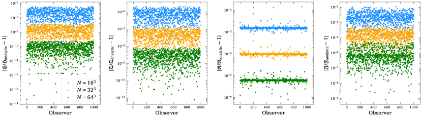
Figure 7 shows the absolute value of the relative error for the effective Hubble, deceleration, curvature, and jerk parameters (panels, left-to-right, respectively). Points show (47) averaged over all lines of sight for a single observer. Blue points are for a $16^{3}$ grid, yellow for a $32^{3}$ grid, and green for a $64^{3}$ grid. The relative error remains below 1% for the effective curvature parameter, below 0.1% for the effective jerk parameter, and below $10^{-4}$% for the effective Hubble and deceleration parameters, even for the coarse resolutions used here.

The errors in these calculations should reduce at a rate defined by the order of accuracy of the scheme used when increasing the resolution. The rate of convergence, $C$, for a set of errors at three resolutions is calculated as, e.g. for the Hubble parameter,

$$C(\mathfrak{H})\equiv\frac{{\rm err(\mathfrak{H})_{low}}-{\rm err(\mathfrak{H})_{mid}}}{{\rm err(\mathfrak{H})_{mid}}-{\rm err(\mathfrak{H})_{high}}},$$ (48)

where a subscript ‘low’ refers to the error for the lowest resolution, ‘mid’ for the middle resolution, and ‘high’ for the highest resolution. For fourth-order accurate derivatives, and when doubling the resolution for each increase, the expected rate of convergence is $C_{\rm exp}=16$.

Figure 8: Convergence rate (48) relative to the expected value, $C/C_{\rm exp}$, for the effective Hubble, deceleration, curvature, and jerk parameters (panels, left-to-right, respectively). The convergence here is for the errors shown in Figure 7 at resolutions $16^{3},32^{3}$, and $64^{3}$.

Figure 8 shows the convergence rate (48), relative to the expected value, for the errors in the effective cosmological parameters shown in Figure 7. All parameters show the expected rate of convergence for fourth-order accurate calculations.

Appendix C Numerical convergence and error bars

In the previous section we assessed the level of error in the mescaline calculations alone, excluding any additional numerical error associated with performing NR simulations. Our main results will contain additional sources of error to those addressed in the previous section. Here we compare simulations at several resolutions to assess convergence and quantify the error bars on our main results.

We note that the simulations used in this Appendix contain an error in the initial data Macpherson and Heinesen [see 72, for details], however this does not change the numerical convergence properties of the simulations. Fixing this error changes the power spectrum of the initial data, with no effect on the evolution of the simulations and therefore convergence properties will remain unchanged. For this reason we did not consider it necessary to re-run these convergence tests. However, we note this here because the variances presented in these controlled-mode simulations are larger than the main results, due to their higher typical density contrasts.

The simulations presented here use the Einstein Toolkit paired with FLRWSolver for initial data. Our numerical setup is the same as presented in Macpherson et al. [40], except that we use different power spectra for the initial conditions. We use the BSSNOK formalism to evolve our cosmological space-times, which means the constraint equations are not explicitly enforced as a part of this evolution. The level of violation in the constraints therefore tells us how closely our simulations are matching a solution of Einstein’s equations. Any violation arises either as a result of constraint violation in the initial data, or numerical error produced during the simulation. We assume linear perturbations in our initial conditions, and therefore we have an initial violation of size second-order in the perturbations. We expect the violation due to numerical error will dominate by the end of the simulation. We use mescaline to calculate the $L_{1}$ norm of the dimensionless Hamiltonian constraint violation, which for the $N=128$ simulations with 100 (200) $h^{-1}$ Mpc smoothing lengths we find to be $0.6\%$ ($1.1\%$). We refer the reader to Macpherson et al. [40] for further details on the constraint violation and studies on its convergence in a set of simulations using the same numerical methods as used here.

C.1 Controlled-mode simulations

We perform simulations at 3 different numerical resolutions to calculate error bars for our main results via a Richardson extrapolation. The Richardson extrapolation method requires keeping the physical system in question fixed with the change of resolution, such that the error associated with the numerical resolution can be isolated. The simulation shown in Figure 1, and any others quoted in the main text, represent a “full” power spectrum sampling, i.e. the initial data contains modes down to the minimum possible wavelength (equal to the physical scale spanned by 2 grid cells). As we increase numerical resolution (reduce the size of grid cells) we therefore change the physical local structure at each observer’s position. These simulations are thus not suitable for a Richardson extrapolation.

Therefore, as in [40], we perform a set of simulations in which small-scale structure is removed from the initial data, and only long-wavelength modes are sampled initially [see also 73, 31]. If these modes are sufficiently large, we expect the structures at all points in the domain to remain similar between resolutions. We perform three simulations with domain length 2 $h^{-1}$ Gpc at resolution $N^{3}$ for $N=32,64$, and $128$, in which we have excluded any power at scales below $10\Delta_{x,32}$, where $\Delta_{x,32}$ is the grid spacing for the $N=32$ simulation. Higher resolution initial data is obtained by interpolating the lower-resolution data. The minimum modes therefore have wavelength $\sim 625h^{-1}$ Mpc in all initial data.

Figure 9: Density (left panel) and expansion rate (right panel) for our $N=64$ test simulation used to perform a Richardson extrapolation of our results. We show a 2–dimensional slice through the domain at $z_{\rm eff}=0$, for a $2h^{-1}{\rm Gpc}$ domain length.

As an example, Figure 9 shows a 2–dimensional slice through the $N=64$ test simulation, with the density field, $\rho$, in the left panel and the expansion scalar, $\theta$, in the right panel.

One might consider using simulations such as this for the main results presented in this paper. While we do restrict the minimum mode to wavelength $\sim 625h^{-1}$ Mpc for the initial data for the simulations described in this appendix, there is no guarantee that structures below this scale will not form later in the simulation. In this work, we wish to strictly constrain any structures to be above the smoothing scale of interest, which is why we choose individual grid cells to coincide with this scale. However, we confirm that the effective parameters are qualitatively similar in the controlled-mode simulations when sampling similar physical scales.

C.2 Richardson extrapolation and definition of error

We expect that our numerical estimates of physical quantities of interest will approach the “true” values of the quantities (in the context of the approximations and limitations of the simulations used) as we increase numerical resolution towards infinity, i.e., $N\rightarrow\infty$. The rate at which an estimated quantity will approach its “true” value depends on the accuracy of the implemented scheme (i.e., how the error reduces as we increase resolution). The Einstein Toolkit thorns which we use are fourth-order accurate (as is mescaline), and we therefore expect our numerical estimates to converge at a rate $\propto N^{-4}$. Thus, we estimate the numerical error of a quantity by calculating the same quantity at three different resolutions, and fitting a curve of the form $f(N)=a+b/N^{4}$, where $a$ and $b$ are parameters determined using the SciPy package’s curve_fit function. Extrapolating the quantity to very large $N$ by using the determined function $N\mapsto f(N)$ (here we choose $N=10^{5}$, which ensures that the value is stable) gives an estimate of the “true” value of that quantity. We then define the error in, e.g., $\mathfrak{H}$ as the residual between our highest-resolution calculation and the extrapolated “true” value, normalised by the mean magnitude of $\mathfrak{H}$, namely,

$$\mathfrak{H}\;{\rm error}\equiv\frac{\mathfrak{H}(N=128)-\mathfrak{H}_{\rm extrap}(N=10^{5})}{{\rm mean}(|\mathfrak{H}(N=128)|)}.$$ (49)

Normalising the error in this way produces an estimate on the relative error while avoiding spurious large-magnitude errors caused by near-zero values (especially relevant for those parameters with distributions centred around zero).

In the controlled simulations described in the previous section, we calculate the effective cosmological parameters (6) at 1000 observer positions, keeping these positions constant between resolutions. For each observer, we randomly choose 300 lines of sight across the whole observer’s sky (‘FullSky’ in Figure 2(a)). The direction vector $e^{\mu}$ for each line of sight, for each observer, is determined using the same random numbers $m^{i}$ (see Appendix B.3) between resolutions. However, in order to ensure the orthonormality requirements (27), we require the 3–metric and fluid 4–velocity at each location to determine $e^{\mu}$ from $m^{i}$. Therefore, the direction vectors do vary slightly between resolutions, however, we confirm that the components of $e^{\mu}$ generally converge at the expected fourth-order rate.

Figure 10: Example of the Richardson extrapolation process for effective Hubble, deceleration, and curvature parameters (panels, left-to-right, respectively) for controlled-mode simulations with resolutions $N=32,64,$ and $128$ (x-axis). Points are calculations from the simulations averaged over 1000 observers, and dashed curves are the best-fit curves representing fourth-order convergence.

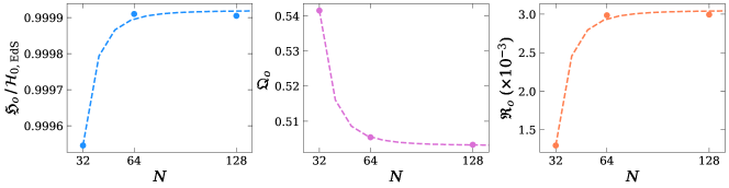
We average the effective anisotropic cosmological parameters of each observer over all 300 lines of sight, and compare this average between resolutions using a Richardson extrapolation. We also assess the convergence of the parameters averaged over all 1000 observers. Figure 10 shows an example of this process for the effective Hubble, deceleration, and curvature parameters (panels, left-to-right, respectively, see Appendix C.5 below for a discussion on the error in the jerk parameter) for the average over all 1000 observers. Points show calculations from simulations at resolution $N$ (x-axis) and dashed curves are the best-fit representing fourth-order convergence. The asymptotic values in Figure 10 can be interpreted as reflecting the expected “true” values for each parameter (for a particular coarse-graining scale), i.e. at infinite numerical resolution. We note that we do not necessarily expect these asymptotic values to correspond to their EdS counterparts, since the points themselves represent different numerical resolutions, and not different coarse-graining scales. We can interpret each point in Figure 10 in the same way as the horizontal lines in, e.g. Figure 5 (or Figure 12), i.e. the average over all observers. We further stress that the non-zero asymptotic value of the effective curvature parameter, in the right-most panel of Figure 10, is not necessarily indicative of a non-zero averaged spatial curvature in the simulation. This is due to the fact the interpretation of the generalised curvature parameter is not simply connected to the averaged Ricci curvature of spatial sections, as it is in the FLRW cosmography [see 26].

C.3 Error calculation in controlled-mode simulations

Figure 11: Percentage relative error (49) for effective Hubble, deceleration, and jerk parameters (panels, left-to-right) calculated via a Richardson extrapolation. Points show the error in calculations averaged over 300 lines of sight for each observer, and black dashed lines in each panel show the average error over all 1000 observers.

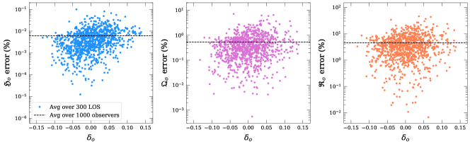
Panels, left-to-right, in Figure 11 show the error (49) for the effective Hubble, deceleration, and curvature parameters, respectively, as a function of the local over-density at the observer, $\delta_{o}$. Points show the error in an observers line-of-sight average measurement, and dashed black lines show the average error over all observers, which yield $\sim 0.006\%$, $\sim 0.5\%$, and $\sim 4.6\%$ for the effective Hubble, deceleration, and curvature parameters, respectively. See Section C.5 below for a discussion on the error in the jerk parameter. The controlled-mode simulations used to quantify these errors are sampling similar physical scales at $z_{\rm eff}=0$ (of the order of hundreds of Mpc), and so we take the errors shown in Figure 11 to be representative of the level of error in our main results.

As mentioned above, there is no guarantee that smaller-scale structures will not develop in these controlled-mode simulations. This also implies that differences in structure growth between resolutions are possible. In turn, not all observers will necessarily have similar enough local environments, and in these cases we expect that calculations will not converge. This can simply be because differences between resolutions are no longer purely due to truncation error in the finite difference approximation of derivatives.

This appears to be the cause of the largest-magnitude errors in all parameters shown in Figure 11. Specifically, we find that for observers with the largest errors — mainly coinciding with non-convergence of the respective parameter —, the local density $\delta_{o}$ also does not converge. This indicates that the structure is physically different between resolutions at the position of these observers and therefore a meaningful comparison between resolutions is difficult.

C.4 Statistical convergence

As detailed above, in order to obtain convergence for an individual observer we require the local structure at that observer’s position to remain constant as we increase resolution. However, as long as the simulations in question continue to sample the same physical smoothing scale, we expect to see statistically similar results across all observers, even when increasing numerical resolution. In this section, we ensure that our main results exhibit statistical convergence in this sense.

We perform three simulations each with a coarse-graining scale of 200 $h^{-1}$ Mpc, with resolutions $N=32,64$, and $128$. The highest resolution of this set is the main simulation presented in Figure 1. Since we must maintain the same minimum scales sampled, with each $2\times$ increase in resolution we also increase the total (physical) domain size by a factor of 2. The simulation box sizes are therefore $6.4,12.8$, and $25.6h^{-1}$ Gpc, respectively. The size of the box in code units remains the same for all simulations in this study, and all initial data are different realisations of the same power spectrum.

Figure 12: Effective cosmological parameters for 3 simulations at different numerical resolution (different coloured points and lines), all with the same physical smoothing length of 200 $h^{-1}$ Mpc. This figure shows the same as Figure 5 for multiple resolutions sampling the same physical scale.

Points in Figure 12 show the effective cosmological parameters (6) as measured by 1000 observers (each averaged over 300 ‘FullSky’ lines of sight) in these three simulations (different colours, as indicated in the legend). Dashed lines of the same colour show the average over all observers for each resolution. Qualitatively, we notice the distribution in each parameter does not change drastically with resolution. We perform a Kolmogorov-Smirnov (KS) test to assess the null hypothesis that parameter distributions between resolutions $N=64$ and $128$ are drawn from the same distribution. We find that the KS test fails to reject the null hypothesis at significance level $\alpha=0.15$. We therefore conclude that the results presented in the main text regarding statistics across all observers are robust to changes in resolution.

C.5 Error in the jerk parameter

For the controlled-mode simulations discussed in the previous sections, we did not find the expected convergence of the effective jerk parameter, $\mathfrak{J}_{o}$. We found that for $\sim 15\%$ of observers, $\mathfrak{J}_{o}$ is well-behaved and converges at the expected fourth-order rate. For these observers the maximum relative error in $\mathfrak{J}_{o}$ is $\sim 5\%$. However, for most observers, and therefore for the average over all observers, we do not see convergence.

We have attributed this to differences in the local density gradients at late times, which, as discussed in the previous sections, can be slightly different between resolutions. We confirm that the jerk parameter converges at the expected fourth-order rate at earlier times in the simulations, when gradients are more similar between resolutions. We also refer the reader to Section B.4, where $\mathfrak{J}_{o}$ converges as expected in an analytic test where gradients are constructed to be exactly identical between resolutions. We note that for the observers who do not show convergence at late times, we also do not see convergence of the local density, $\delta_{o}$, whereas for those 15% who do show convergence, the local density also converges. This strongly suggests the main reason for this is due to differences in the local density field. The dominant contribution to the jerk parameter is the second derivative of $\mathfrak{H}$ along the null ray (i.e., third derivatives of the fluid velocity). If local structure is slightly different between resolutions this will be more noticeable in the calculation of higher-order derivatives. This explains both why we see convergence in $\mathfrak{J}_{o}$ at earlier times, and why we see convergence of other parameters (which have dominant contributions from lower-order derivatives) at late times.

Since we cannot quantify error bars on $\mathfrak{J}_{o}$ in a controlled simulation that is still physically similar to our main results, we choose to avoid making statements on the jerk parameter for individual observers. From the results of the KS test presented in the previous section, the distribution of the jerk parameter across all observers exhibits convergence.

References

- Planck Collaboration et al. [2020] Planck Collaboration, N. Aghanim, Y. Akrami, M. Ashdown, J. Aumont, C. Baccigalupi, M. Ballardini, A. J. Banday, R. B. Barreiro, N. Bartolo, S. Basak, et al., Planck 2018 results. V. CMB power spectra and likelihoods, A&A 641, A5 (2020), arXiv:1907.12875 [astro-ph.CO] .
- Beutler et al. [2011] F. Beutler, C. Blake, M. Colless, D. H. Jones, L. Staveley-Smith, L. Campbell, Q. Parker, W. Saunders, and F. Watson, The 6dF Galaxy Survey: baryon acoustic oscillations and the local Hubble constant, MNRAS 416, 3017 (2011), arXiv:1106.3366 [astro-ph.CO] .
- Alam et al. [2017] S. Alam, M. Ata, S. Bailey, F. Beutler, D. Bizyaev, J. A. Blazek, A. S. Bolton, J. R. Brownstein, A. Burden, C.-H. Chuang, J. Comparat, et al., The clustering of galaxies in the completed SDSS-III Baryon Oscillation Spectroscopic Survey: cosmological analysis of the DR12 galaxy sample, MNRAS 470, 2617 (2017), arXiv:1607.03155 [astro-ph.CO] .
- Riess et al. [2007] A. G. Riess, L.-G. Strolger, S. Casertano, H. C. Ferguson, B. Mobasher, B. Gold, P. J. Challis, A. V. Filippenko, S. Jha, W. Li, J. Tonry, et al., New Hubble Space Telescope Discoveries of Type Ia Supernovae at z >= 1: Narrowing Constraints on the Early Behavior of Dark Energy, ApJ 659, 98 (2007), arXiv:astro-ph/0611572 [astro-ph] .
- Abbott et al. [2019] T. M. C. Abbott, S. Allam, P. Andersen, C. Angus, J. Asorey, A. Avelino, S. Avila, B. A. Bassett, K. Bechtol, G. M. Bernstein, E. Bertin, et al., First Cosmology Results using Type Ia Supernovae from the Dark Energy Survey: Constraints on Cosmological Parameters, ApJ 872, L30 (2019), arXiv:1811.02374 [astro-ph.CO] .
- Riess et al. [2018] A. G. Riess, S. Casertano, W. Yuan, L. Macri, J. Anderson, J. W. MacKenty, J. B. Bowers, K. I. Clubb, A. V. Filippenko, D. O. Jones, and B. E. Tucker, New Parallaxes of Galactic Cepheids from Spatially Scanning the Hubble Space Telescope: Implications for the Hubble Constant, ApJ 855, 136 (2018), arXiv:1801.01120 [astro-ph.SR] .
- Riess et al. [2019] A. G. Riess, S. Casertano, W. Yuan, L. M. Macri, and D. Scolnic, Large Magellanic Cloud Cepheid Standards Provide a 1% Foundation for the Determination of the Hubble Constant and Stronger Evidence for Physics beyond CDM, Astrophys. J. 876, 85 (2019), arXiv:1903.07603 [astro-ph.CO] .
- Di Valentino et al. [2019] E. Di Valentino, A. Melchiorri, and J. Silk, Planck evidence for a closed Universe and a possible crisis for cosmology, Nature Astron. 4, 196 (2019), arXiv:1911.02087 [astro-ph.CO] .
- Aghanim et al. [2020a] N. Aghanim et al. (Planck), Planck 2018 results. VI. Cosmological parameters, Astron. Astrophys. 641, A6 (2020a), arXiv:1807.06209 [astro-ph.CO] .
- Di Valentino et al. [2021] E. Di Valentino, O. Mena, S. Pan, L. Visinelli, W. Yang, A. Melchiorri, D. F. Mota, A. G. Riess, and J. Silk, In the Realm of the Hubble tension a Review of Solutions, arXiv e-prints , arXiv:2103.01183 (2021), arXiv:2103.01183 [astro-ph.CO] .
- Bernal et al. [2021] J. L. Bernal, L. Verde, R. Jimenez, M. Kamionkowski, D. Valcin, and B. D. Wandelt, Trouble beyond H0 and the new cosmic triangles, Phys. Rev. D 103, 103533 (2021), arXiv:2102.05066 [astro-ph.CO] .
- Di Valentino et al. [2020] E. Di Valentino, L. A. Anchordoqui, O. Akarsu, Y. Ali-Haimoud, L. Amendola, N. Arendse, M. Asgari, M. Ballardini, S. Basilakos, E. Battistelli, M. Benetti, et al., Cosmology Intertwined II: The Hubble Constant Tension, arXiv e-prints , arXiv:2008.11284 (2020), arXiv:2008.11284 [astro-ph.CO] .
- Riess et al. [1998] A. G. Riess, A. V. Filippenko, P. Challis, A. Clocchiatti, A. Diercks, P. M. Garnavich, R. L. Gilliland, C. J. Hogan, S. Jha, R. P. Kirshner, B. Leibundgut, M. M. Phillips, D. Reiss, B. P. Schmidt, R. A. Schommer, R. C. Smith, J. Spyromilio, C. Stubbs, N. B. Suntzeff, and J. Tonry, Observational Evidence from Supernovae for an Accelerating Universe and a Cosmological Constant, Astron. J. 116, 1009 (1998), arXiv:astro-ph/9805201 [astro-ph] .
- Perlmutter et al. [1999] S. Perlmutter, G. Aldering, G. Goldhaber, R. A. Knop, P. Nugent, P. G. Castro, S. Deustua, S. Fabbro, A. Goobar, D. E. Groom, I. M. Hook, A. G. Kim, et al., Measurements of and from 42 High-Redshift Supernovae, ApJ 517, 565 (1999), arXiv:astro-ph/9812133 [astro-ph] .
- Cole et al. [2005] S. Cole et al. (2dFGRS), The 2dF Galaxy Redshift Survey: Power-spectrum analysis of the final dataset and cosmological implications, Mon. Not. Roy. Astron. Soc. 362, 505 (2005), arXiv:astro-ph/0501174 .
- Eisenstein et al. [2005] D. J. Eisenstein et al. (SDSS), Detection of the Baryon Acoustic Peak in the Large-Scale Correlation Function of SDSS Luminous Red Galaxies, Astrophys. J. 633, 560 (2005), arXiv:astro-ph/0501171 .
- Aghanim et al. [2020b] N. Aghanim et al. (Planck), Planck 2018 results. V. CMB power spectra and likelihoods, Astron. Astrophys. 641, A5 (2020b), arXiv:1907.12875 [astro-ph.CO] .
- Amendola et al. [2018] L. Amendola, S. Appleby, A. Avgoustidis, D. Bacon, T. Baker, M. Baldi, N. Bartolo, A. Blanchard, C. Bonvin, S. Borgani, E. Branchini, et al., Cosmology and fundamental physics with the Euclid satellite, Living Reviews in Relativity 21, 2 (2018), arXiv:1606.00180 [astro-ph.CO] .
- Ivezić et al. [2019] Ž. Ivezić, S. M. Kahn, J. A. Tyson, B. Abel, E. Acosta, R. Allsman, D. Alonso, Y. AlSayyad, S. F. Anderson, J. Andrew, J. R. P. Angel, et al., LSST: From Science Drivers to Reference Design and Anticipated Data Products, ApJ 873, 111 (2019), arXiv:0805.2366 [astro-ph] .
- Square Kilometre Array Cosmology Science Working Group et al. [2020] Square Kilometre Array Cosmology Science Working Group, D. J. Bacon, R. A. Battye, P. Bull, S. Camera, P. G. Ferreira, I. Harrison, D. Parkinson, A. Pourtsidou, M. G. Santos, et al., Cosmology with Phase 1 of the Square Kilometre Array Red Book 2018: Technical specifications and performance forecasts, PASA 37, e007 (2020), arXiv:1811.02743 [astro-ph.CO] .
- Scolnic et al. [2019] D. Scolnic, S. Perlmutter, G. Aldering, D. Brout, T. Davis, A. Filippenko, R. Foley, R. Hložek, R. Hounsell, D. Jones, P. Kelly, et al., The Next Generation of Cosmological Measurements with Type Ia Supernovae, Astro2020: Decadal Survey on Astronomy and Astrophysics 2020, 270 (2019), arXiv:1903.05128 [astro-ph.CO] .
- Seitz et al. [1994] S. Seitz, P. Schneider, and J. Ehlers, Light propagation in arbitrary space-times and the gravitational lens approximation, Class. Quant. Grav. 11, 2345 (1994), arXiv:astro-ph/9403056 .
- Kristian and Sachs [1966] J. Kristian and R. K. Sachs, Observations in Cosmology, ApJ 143, 379 (1966).
- Clarkson and Umeh [2011] C. Clarkson and O. Umeh, Is backreaction really small within concordance cosmology?, Class. Quant. Grav. 28, 164010 (2011), arXiv:1105.1886 [astro-ph.CO] .
- Clarkson et al. [2012] C. Clarkson, G. F. R. Ellis, A. Faltenbacher, R. Maartens, O. Umeh, and J.-P. Uzan, (Mis-)Interpreting supernovae observations in a lumpy universe, Mon. Not. Roy. Astron. Soc. 426, 1121 (2012), arXiv:1109.2484 [astro-ph.CO] .
- Heinesen [2020] A. Heinesen, Multipole decomposition of the general luminosity distance ’Hubble law’ – a new framework for observational cosmology, arXiv e-prints , arXiv:2010.06534 (2020), arXiv:2010.06534 [astro-ph.CO] .
- Giblin et al. [2016a] J. T. Giblin, J. B. Mertens, and G. D. Starkman, Departures from the Friedmann-Lemaitre-Robertston-Walker Cosmological Model in an Inhomogeneous Universe: A Numerical Examination, Phys. Rev. Lett. 116, 251301 (2016a), arXiv:1511.01105 [gr-qc] .
- Bentivegna and Bruni [2016] E. Bentivegna and M. Bruni, Effects of nonlinear inhomogeneity on the cosmic expansion with numerical relativity, Phys. Rev. Lett. 116, 251302 (2016), arXiv:1511.05124 [gr-qc] .
- Macpherson et al. [2017] H. J. Macpherson, P. D. Lasky, and D. J. Price, Inhomogeneous Cosmology with Numerical Relativity, Phys. Rev. D 95, 064028 (2017), arXiv:1611.05447 [astro-ph.CO] .
- East et al. [2018] W. E. East, R. Wojtak, and T. Abel, Comparing Fully General Relativistic and Newtonian Calculations of Structure Formation, Phys. Rev. D 97, 043509 (2018), arXiv:1711.06681 [astro-ph.CO] .
- Daverio et al. [2019] D. Daverio, Y. Dirian, and E. Mitsou, General relativistic cosmological N-body simulations. Part I. Time integration, J. Cosmology Astropart. Phys 2019, 065 (2019), arXiv:1904.07841 [astro-ph.CO] .
- Visser [2004] M. Visser, Jerk and the cosmological equation of state, Class. Quant. Grav. 21, 2603 (2004), arXiv:gr-qc/0309109 .
- Weinberg [1972] S. Weinberg, Gravitation and Cosmology: Principles and Applications of the General Theory of Relativity (1972).
- Löffler et al. [2012] F. Löffler, J. Faber, E. Bentivegna, T. Bode, P. Diener, R. Haas, I. Hinder, B. C. Mundim, C. D. Ott, E. Schnetter, G. Allen, M. Campanelli, and P. Laguna, The Einstein Toolkit: a community computational infrastructure for relativistic astrophysics, Classical and Quantum Gravity 29, 115001 (2012), arXiv:1111.3344 [gr-qc] .
- Zilhão and Löffler [2013] M. Zilhão and F. Löffler, An Introduction to the Einstein Toolkit, International Journal of Modern Physics A 28, 1340014-126 (2013), arXiv:1305.5299 [gr-qc] .
- Nakamura et al. [1987] T. Nakamura, K. Oohara, and Y. Kojima, General Relativistic Collapse to Black Holes and Gravitational Waves from Black Holes, Progress of Theoretical Physics Supplement 90, 1 (1987).
- Baumgarte and Shapiro [1999] T. W. Baumgarte and S. L. Shapiro, Numerical integration of Einstein’s field equations, Phys. Rev. D 59, 024007 (1999), arXiv:gr-qc/9810065 [gr-qc] .
- Shibata and Nakamura [1995] M. Shibata and T. Nakamura, Evolution of three-dimensional gravitational waves: Harmonic slicing case, Phys. Rev. D 52, 5428 (1995).
- Bentivegna [2017] E. Bentivegna, An automatically generated code for relativistic inhomogeneous cosmologies, Phys. Rev. D 95, 044046 (2017), arXiv:1610.05198 [gr-qc] .
- Macpherson et al. [2019] H. J. Macpherson, D. J. Price, and P. D. Lasky, Einstein’s Universe: Cosmological structure formation in numerical relativity, Phys. Rev. D 99, 063522 (2019), arXiv:1807.01711 [astro-ph.CO] .
- Wang [2018] K. Wang, Numerical relativity investigation of the effects of gravitational waves on the inhomogeneity of the universe, Eur. Phys. J. C 78, 629 (2018), arXiv:1801.08362 [astro-ph.CO] .
- Brown et al. [2009] D. Brown, P. Diener, O. Sarbach, E. Schnetter, and M. Tiglio, Turduckening black holes: An analytical and computational study, Phys. Rev. D 79, 044023 (2009), arXiv:0809.3533 [gr-qc] .
- Baiotti et al. [2005] L. Baiotti, I. Hawke, P. J. Montero, F. Löffler, L. Rezzolla, N. Stergioulas, J. A. Font, and E. Seidel, Three-dimensional relativistic simulations of rotating neutron-star collapse to a Kerr black hole, Phys. Rev. D 71, 024035 (2005), arXiv:gr-qc/0403029 [gr-qc] .
- Mösta et al. [2014] P. Mösta, B. C. Mundim, J. A. Faber, R. Haas, S. C. Noble, T. Bode, F. Löffler, C. D. Ott, C. Reisswig, and E. Schnetter, GRHydro: a new open-source general-relativistic magnetohydrodynamics code for the Einstein toolkit, Classical and Quantum Gravity 31, 015005 (2014), arXiv:1304.5544 [gr-qc] .
- Macpherson et al. [2018] H. J. Macpherson, P. D. Lasky, and D. J. Price, The trouble with Hubble: Local versus global expansion rates in inhomogeneous cosmological simulations with numerical relativity, Astrophys. J. 865, L4 (2018), arXiv:1807.01714 [astro-ph.CO] .
- Hogg et al. [2005] D. W. Hogg, D. J. Eisenstein, M. R. Blanton, N. A. Bahcall, J. Brinkmann, J. E. Gunn, and D. P. Schneider, Cosmic homogeneity demonstrated with luminous red galaxies, Astrophys. J. 624, 54 (2005), arXiv:astro-ph/0411197 .
- Scrimgeour et al. [2012] M. I. Scrimgeour, T. Davis, C. Blake, J. B. James, G. B. Poole, L. Staveley-Smith, S. Brough, M. Colless, C. Contreras, W. Couch, S. Croom, et al., The WiggleZ Dark Energy Survey: the transition to large-scale cosmic homogeneity, MNRAS 425, 116 (2012), arXiv:1205.6812 [astro-ph.CO] .
- Blas et al. [2011] D. Blas, J. Lesgourgues, and T. Tram, The Cosmic Linear Anisotropy Solving System (CLASS). Part II: Approximation schemes, J. Cosmology Astropart. Phys 2011, 034 (2011), arXiv:1104.2933 [astro-ph.CO] .
- Riess et al. [2016] A. G. Riess, L. M. Macri, S. L. Hoffmann, D. Scolnic, S. Casertano, A. V. Filippenko, B. E. Tucker, M. J. Reid, D. O. Jones, J. M. Silverman, R. Chornock, P. Challis, W. Yuan, P. J. Brown, and R. J. Foley, A 2.4% Determination of the Local Value of the Hubble Constant, ApJ 826, 56 (2016), arXiv:1604.01424 [astro-ph.CO] .
- Rasanen [2009] S. Rasanen, Light propagation in statistically homogeneous and isotropic dust universes, JCAP 02, 011, arXiv:0812.2872 [astro-ph] .
- Rasanen [2010] S. Rasanen, Light propagation in statistically homogeneous and isotropic universes with general matter content, JCAP 03, 018, arXiv:0912.3370 [astro-ph.CO] .
- Górski et al. [2005] K. M. Górski, E. Hivon, A. J. Banday, B. D. Wandelt, F. K. Hansen, M. Reinecke, and M. Bartelmann, HEALPix: A Framework for High-Resolution Discretization and Fast Analysis of Data Distributed on the Sphere, ApJ 622, 759 (2005), arXiv:astro-ph/0409513 [astro-ph] .
- Andrade et al. [2018] U. Andrade, C. A. P. Bengaly, B. Santos, and J. S. Alcaniz, A Model-independent Test of Cosmic Isotropy with Low-z Pantheon Supernovae, ApJ 865, 119 (2018), arXiv:1806.06990 [astro-ph.CO] .
- Kalus et al. [2013] B. Kalus, D. J. Schwarz, M. Seikel, and A. Wiegand, Constraints on anisotropic cosmic expansion from supernovae, A&A 553, A56 (2013), arXiv:1212.3691 [astro-ph.CO] .
- Bengaly et al. [2015] J. Bengaly, C. A. P., A. Bernui, and J. S. Alcaniz, Probing Cosmological Isotropy with Type Ia Supernovae, ApJ 808, 39 (2015), arXiv:1503.01413 [astro-ph.CO] .
- Bengaly [2016] J. Bengaly, C. A. P., Constraining the local variance of H0 from directional analyses, J. Cosmology Astropart. Phys 2016, 036 (2016), arXiv:1510.05545 [astro-ph.CO] .
- Colin et al. [2019] J. Colin, R. Mohayaee, M. Rameez, and S. Sarkar, Evidence for anisotropy of cosmic acceleration, Astron. Astrophys. 631, L13 (2019), arXiv:1808.04597 [astro-ph.CO] .
- Bolejko et al. [2016] K. Bolejko, M. A. Nazer, and D. L. Wiltshire, Differential cosmic expansion and the Hubble flow anisotropy, JCAP 06, 035, arXiv:1512.07364 [astro-ph.CO] .
- Migkas et al. [2020] K. Migkas, G. Schellenberger, T. H. Reiprich, F. Pacaud, M. E. Ramos-Ceja, and L. Lovisari, Probing cosmic isotropy with a new X-ray galaxy cluster sample through the scaling relation, Astron. Astrophys. 636, A15 (2020), arXiv:2004.03305 [astro-ph.CO] .
- Marra et al. [2013] V. Marra, L. Amendola, I. Sawicki, and W. Valkenburg, Cosmic Variance and the Measurement of the Local Hubble Parameter, Phys. Rev. Lett. 110, 241305 (2013), arXiv:1303.3121 [astro-ph.CO] .
- Camarena and Marra [2018] D. Camarena and V. Marra, Impact of the cosmic variance on H0 on cosmological analyses, Phys. Rev. D 98, 023537 (2018), arXiv:1805.09900 [astro-ph.CO] .
- Wojtak et al. [2014] R. Wojtak, A. Knebe, W. A. Watson, I. T. Iliev, S. Heß, D. Rapetti, G. Yepes, and S. Gottlöber, Cosmic variance of the local Hubble flow in large-scale cosmological simulations, MNRAS 438, 1805 (2014), arXiv:1312.0276 [astro-ph.CO] .
- Odderskov et al. [2014] I. Odderskov, S. Hannestad, and T. Haugbølle, On the local variation of the Hubble constant, J. Cosmology Astropart. Phys 2014, 028 (2014), arXiv:1407.7364 [astro-ph.CO] .
- Wu and Huterer [2017] H.-Y. Wu and D. Huterer, Sample variance in the local measurements of the Hubble constant, MNRAS 471, 4946 (2017), arXiv:1706.09723 [astro-ph.CO] .
- Adamek et al. [2016] J. Adamek, D. Daverio, R. Durrer, and M. Kunz, General relativity and cosmic structure formation, Nature Phys. 12, 346 (2016), arXiv:1509.01699 [astro-ph.CO] .
- Adamek et al. [2016] J. Adamek, D. Daverio, R. Durrer, and M. Kunz, gevolution: a cosmological N-body code based on General Relativity, J. Cosmology Astropart. Phys 2016, 053 (2016), arXiv:1604.06065 [astro-ph.CO] .
- Adamek et al. [2019] J. Adamek, C. Clarkson, L. Coates, R. Durrer, and M. Kunz, Bias and scatter in the Hubble diagram from cosmological large-scale structure, Phys. Rev. D 100, 021301 (2019), arXiv:1812.04336 [astro-ph.CO] .
- Barrera-Hinojosa and Li [2020] C. Barrera-Hinojosa and B. Li, GRAMSES: a new route to general relativistic -body simulations in cosmology - I. Methodology and code description, JCAP 2001 (01), 007, arXiv:1905.08890 [astro-ph.CO] .
- Barrera-Hinojosa and Li [2020] C. Barrera-Hinojosa and B. Li, GRAMSES: a new route to general relativistic N-body simulations in cosmology. Part II. Initial conditions, J. Cosmology Astropart. Phys 2020, 056 (2020), arXiv:2001.07968 [astro-ph.CO] .
- Carlesi et al. [2016] E. Carlesi et al., Constrained Local UniversE Simulations: A Local Group Factory, Mon. Not. Roy. Astron. Soc. 458, 900 (2016), arXiv:1602.03919 [astro-ph.CO] .
- Cattoen and Visser [2007] C. Cattoen and M. Visser, The Hubble series: Convergence properties and redshift variables, Class. Quant. Grav. 24, 5985 (2007), arXiv:0710.1887 [gr-qc] .
- Macpherson and Heinesen [2021] H. J. Macpherson and A. Heinesen, Erratum: Luminosity distance and anisotropic sky-sampling at low redshifts: A numerical relativity study [Phys. Rev. D 104, 023525 (2021)], Phys. Rev. D 104, 109901 (2021).
- Giblin et al. [2016b] J. T. Giblin, J. B. Mertens, and G. D. Starkman, Observable Deviations from Homogeneity in an Inhomogeneous Universe, Astrophys. J. 833, 247 (2016b), arXiv:1608.04403 [astro-ph.CO] .