Coexistence of Communications and Cognitive MIMO Radar: Waveform Design and Prototype

Abstract

New generation of radar systems will need to coexist with other radio frequency (RF) systems, anticipating their behavior and reacting appropriately to avoid interference. In light of this requirement, this paper designs, implements, and evaluates the performance of phase-only sequences (with constant power) for intelligent spectrum utilization using the custom built cognitive Multiple Input Multiple Output (MIMO) radar prototype. The proposed transmit waveforms avoid the frequency bands occupied by narrowband interferers or communication links, while simultaneously have a small cross-correlation among each other to enable their separability at the MIMO radar receiver. The performance of the optimized set of sequences obtained through solving a non-convex bi-objective optimization problem, is compared with the state-of-the-art counterparts, and its applicability is illustrated by the developed prototype. A realistic Long Term Evolution (LTE) downlink is used for the communications, and the real-time system implementation is validated and evaluated through the throughput calculations for communications and the detection performance measurement for the radar system.

I Introduction

Spectrum congestion has become an imminent problem with multitude of radio services like wireless communications, active Radio-Frequency (RF) sensing and radio astronomy vying for the scarce usable spectrum. Within this conundrum of spectrum congestion, radars need to cope with simultaneous transmissions from other RF systems. Spectrum sharing with communications being the highly plausible scenario given the need for high bandwidth in both systems [1, 2, 3]. While elaborate allocation policies are in place to regulate the spectral usage, the rigid allocations result in inefficient spectrum utilization when the subscription is sparse. In this context, smart spectrum utilization offers a flexible and a fairly promising solution for improved system performance in the emerging smart sensing systems [4].

Two paradigms, Cognition and Multiple Input Multiple Output (MIMO) have been central to the prevalence of smart sensing systems. Herein, the former concept offers ability to choose intelligent transmission strategies based on prevailing environmental conditions and a prediction of the behavior of the emitters in the scene, in addition to the now ubiquitous receiver adaptation [5, 6, 7, 8]. The second concept, offers a canvas of transmission strategies to the cognition manager to select from; these strategies exploit waveform diversity and the available degrees of freedom [9, 10]. Smart sensing opens up the possibility of coexistence of radar systems with incumbent communication systems in the earlier mentioned spectrum sharing instance. A representative coexistence scenario is illustrated in Figure 1, where an understanding of the environment is essential for seamless operation of radar systems while opportunistically using the spectrum allocated to communication [11, 1, 2, 12].

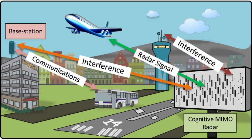
Figure 1: An illustration of coexistence between radar and communications. The radar aims to detect the airplane, without creating interference to the communication links, and similarly avoiding interference from the communication links.

In this paper, we design a cognitive MIMO radar system towards fostering coexistence with communications; it involves spectrum sensing and transmission strategies adapted to the sensed spectrum while accomplishing the radar tasks and without degrading the performance of communications. Particularly, a set of transmit sequences is designed to focus the emitted energy in the bands suggested by the spectrum sensing module while limiting the out-of-band interference. The waveforms, along with the receive processing, are designed to enhance the radar detection performance. The designed system is then demonstrated for the representative scenario of Figure 1 using a custom built Software-Defined Radio (SDR) based prototype developed on Universal Software Radio Peripheral (USRP) s from National Instruments (NI) [13, 14]. These USRP s operate at sub-$6$ GHz frequencies with a maximum instantaneous bandwidth of $160$ MHz.

I-A Background and Related Works

Coexistence of Communication Systems

Spectral coexistence has been found to be a promising method to alleviate the spectrum scarcity problem. For example, in the ISM band, several wireless standards operate on overlapping frequency bands such as the IEEE 802.11 (popularly known as Wi-Fi) and the IEEE 802.15.4 (popularly known as ZigBee) family of standards in the $2.4$ GHz ISM band. As the ISM band does not require a license to transmit, the participating standards transmit at will (frequency and power) leading to interference and a loss of throughput[15, 16, 17]. Similarly, in the 5 GHz ISM band, it has been speculated that there will be interference between IEEE 802.11n/ac and Long Term Evolution (LTE) [18]. For the two aforementioned interference scenarios, several spectral coexistence methods like successive Interference Cancellation (SIC)[19, 20] for single antenna and Technology Independent Multi-Output (TIMO) [21, 22, 23] for multi-antennas have been proposed.

Radar-Communication Coexistence

The interfered bands, including those occupied by communications, are not useful for the radar system, and traditional radars aim to mitigate these frequencies at their receivers. To avoid energy wasted due to transmissions on these bands while pursuing coexistence applications, research into the transmit strategy of spectrally shaped radar waveforms has been driving coexistence studies since the last decade [24, 25, 26, 27, 28, 29, 30, 31, 32]. In fact, it is possible to radiate the radar waveform in a smart way by using two key elements of the cognition; spectrum sensing and spectrum sharing [33, 7]. Further, it is possible to increase the total radar bandwidth, and consequently improve the range resolution by combining several clear bands together [24].

Radar Waveform Optimization for Coexistence

To enable waveform design in coexistence scenarios, several optimization methods including alternative optimization, Majorization-Minimization (MM), Coordinate Descent (CD), Alternating Direction Method of Multipliers (ADMM), power like iterations, etc., have been developed recently for designing waveforms exhibiting deep notches on their spectrum. Herein, we provide a brief summary of the recent works and refer the interested readers to [24, 34, 25, 35, 26, 27, 36, 37, 38, 39, 30, 40, 32, 41, 42] and references therein for an elaborate literature on spectral shaping optimization.

Spectral/ Template Matching: In [25, 26, 27, 37, 38, 41, 42] spectral/template matching approach is pursued to shape the spectral behaviour of the transmit sequences. The approach of template matching is also used in [27] for designing sequences with a specific auto-correlation function, by considering a weighted objective of the both spectral and auto-correlation functions. However, matching to a template in the vicinity of the spectrum edges may decrease the possibility of synthesizing deep notches in the undesired frequency bands.

Signal to Interference plus Noise Ratio (SINR) optimization: In [30, 32], SINR enhancement is considered to design the transmit sequences, while the spectral behaviour is considered as a constraint. Particularly, in [30] mutual information (MI) is maximized based on MM approach while, in [32], a CD based technique is utilized to maximize the SINR; both consider a local control on the interference energy radiated in each frequency band. Both the SINR and mutual information metrics require a knowledge of the possible location of the targets, which cannot be obtained easily in practice. Further, in case of MIMO radar systems, maximizing MI/ SINR as the only design metric has the drawback of leading to a set of waveforms that are fully correlated, i. e., converting the MIMO radar to a conventional phased-array radar [43].

Stopband/ Passband levels: In [39, 40], the ratio of the maximum stopband level to the minimum passband level is considered as the objective function to shape the spectrum of the transmit waveforms with deeper notches compared to its counterparts. This metric is particularly useful in spectrally dense environments, where only the stopbands and passbands of the interfering signals can be estimated by energy detection, matched filtering or feature detection[6]. However, [39, 40], does not consider the correlation behaviour of the designed sequences towards providing the required orthogonality in MIMO radars.

Orthogonality: Traditionally Integrated Sidelobe Level (ISL) has been used as a metric to design set of approximately orthogonal sequences in a Code Division Multiplexing (CDM)-MIMO radar system, i.e., having small auto- and cross-correlation sidelobes [44, 45, 46, 47, 48, 49, 50, 51, 52, 53, 54]. It has been shown that if a sequence set of size $M$, has atleast one $N$-length sequence, then the ISL lower bound ${\cal{B}}_{\text{ISL}}=N^{2}M(M-1)$, [55, 56, 57, 51], can nearly be met by a set of unimodular sequences generated by the algorithms proposed in [44, 45, 46, 47, 48, 49, 50, 51, 52, 53, 54].

Summary of the Shortcomings in Prior-Art

The well-known notch shaping or SINR enhancement methods do not offer satisfactory performance in terms of simultaneously providing sets of uncorrelated sequences and deep notches in the spectrum. In Figure 2, we show that the Integrated Sidelobe Level Ratio (ISLR) values of different sets of random-phase sequences nearly approach the lower bound on aperiodic ISLR. This fact shows that the traditional ISL may not be an ideal choice for the objective function if the goal is to design set of sequences which provide orthogonality in a MIMO radar system. Furthermore, there are no hardware (HW) prototypes to validate the waveform design in a coexistence context. Our work aims to address these shortcomings.

I-B Contribution

In this paper, following a radar-centric approach, we demonstrate for the first time, a coexistence set-up in incumbent communication bands by optimizing, implementing and validating a complete cognitive MIMO radar prototype.

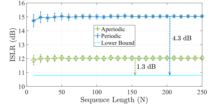
Figure 2: Aperiodic/periodic ISLR values of a set of $M=4$ random-phase sequences averaged over $100$ independent trials: comparison for different sequence lengths.

The key contributions of this paper can be summarized as:

1. Building a SDR based cognitive MIMO radar system capable of performing real-time spectrum sensing and smart spectrum utilization for coexistence in addition to the classical radar tasks like matched filtering and Doppler processing. The testbed implements two-channels achieving a transmitting bandwidth close to $80$ MHz with the possibility of changing the parameters of the processing units during the operation.

2. Setting up of the coexistence system using the aforementioned cognitive MIMO radar and an incumbent LTE link which serves as the communication counterpart.

3. Designing a set of optimized sequences with deep notches in their spectrum that can also be well-separated at the MIMO radar receiver. In this context, we propose an objective function based on the weighted sum Spectral Integrated Level Ratio (SILR) and Integrated Cross Correlation Level (ICCL). These two objectives have been proposed in this paper to encourage the design of waveforms having required spectral as well as cross-correlation properties simultaneously. The optimization is undertaken using the low complexity iterative CD methodology which offers an attractive framework in the context of dynamic spectral shaping. In fact, the SILR renders the CD approach attractive through a simplified single variable optimization.

4. Evaluating and validating the performance of the designed sequences experimentally, through a real-time visualization of the detection performance of the MIMO radar system and a measurement of the LTE throughput. This ensures the development, implementation and validation of one of the first prototypes for co-existing radar and communications with waveform optimization.

I-C Paper Overview and Notation

The rest of the paper is organized as follows. Section II describes the prototype architecture and different applications developed for the demonstration of the coexistence paradigm. Section III describes the proposed optimization of the spectral and cross-correlation of the MIMO radar by defining an novel objective function. In Section IV, the performance of the proposed method is compared with prior-art and the numerical experiments of the USRP implementation of the prototype are given in section V and section VI summarizes the paper. This paper uses lower-case and upper-case boldface for vectors ($a$) and matrices ($A$) respectively. The conjugate, transpose and the conjugate transpose operators are denoted by $(.)^{*}$, $(.)^{T}$ and $(.)^{H}$ respectively. The Frobenius norm, $l_{2}$ norm, absolute value and round operator are denoted by $\mathinner{\!\left\lVert.\right\rVert}_{F}$, $\mathinner{\!\left\lVert.\right\rVert}_{2}$, $|.|$ and $\lfloor.\rceil$ respectively. For a complex number $a$, $\Re(a)$ and $\Im(a)$ denote the real and imaginary part respectively and $j=\sqrt{-1}$. The letter $(i)$ is use as step of a procedure. Finally $\odot$ denotes the Hadamard product.

II The Proposed Prototype Architecture

The prototype consists of three application frameworks as depicted in Figure 3; a) LTE Application Framework, b) Spectrum sensing application, and c) Cognitive MIMO radar application. Various building blocks of the proposed coexistence prototype are shown in Figure 4(b). The HW consists of three main modules: 1) USRP 2974 for LTE communications 2) USRP B210 for spectrum sensing, and 3) USRP 2944R for cognitive MIMO radar with specifications given in TABLE I. The design details of each module are presented in the sequel. USRP s are used for the transmission and reception of the wireless RF signals and the Rohde and Schwarz spectrum analyzer is used for the validation of the transmission.

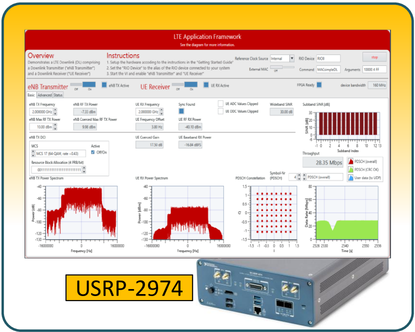
(a) LTE Application

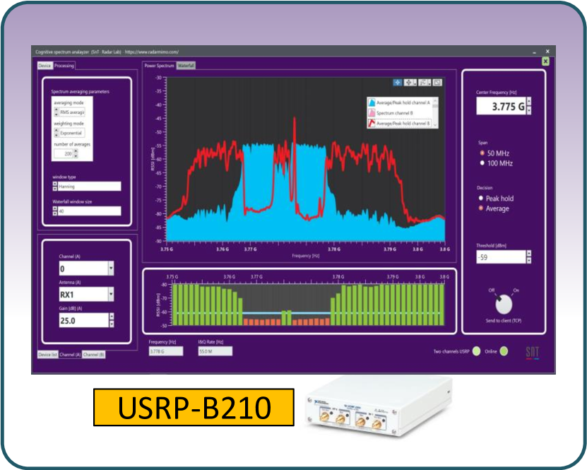
(b) Spectrum Sensing

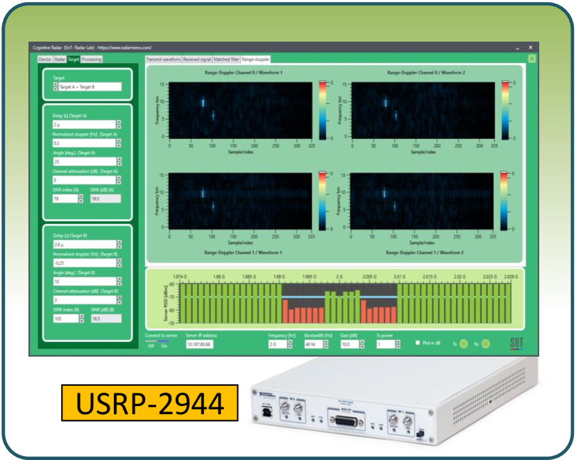
(c) MIMO Radar

Figure 3: Application frameworks forming the proposed prototype: LTE application developed by NI, spectrum sensing and cognitive MIMO radar applications developed in this paper.

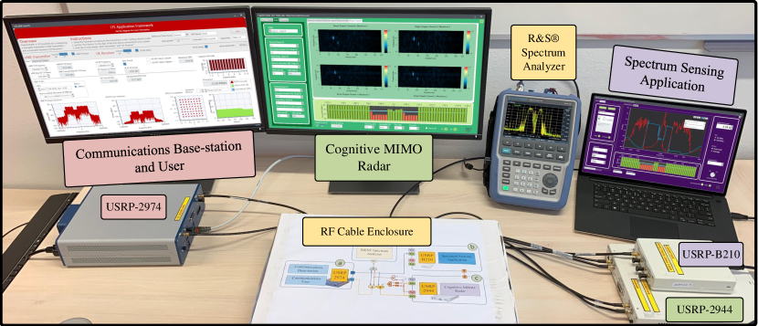
(a)

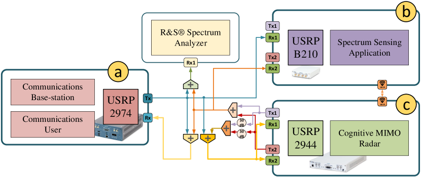
(b)

Figure 4: The photograph (a) and connection diagram (b) and of the proposed coexistence prototype. The photo shows communication BS and user, spectrum sensing, and cognitive MIMO radar systems.

II-A LTE Application Framework

The LabVIEW LTE Application Framework (Figure 3(a)) is an add-on software that provides a real-time physical layer LTE implementation in the form of an open and modifiable source-code [58]. The framework complies with a selected subset of the 3GPP LTE which includes a closed-loop OTA operation with channel state and ACK/ NACK feedback, $20$ MHz bandwidth, Physical Downlink Shared Channel (PDSCH) and Physical Downlink Control Channel (PDCCH), up to $75$ Mbps data throughput, FDD and TDD configuration $5$-frame structure, QPSK, $16$-QAM, and $64$-QAM modulation, channel estimation and zero-forcing channel equalization. The framework also has a basic MAC implementation to enable packet-based data transmission along with a MAC adaptation framework for rate adaptation. Since the NI-USRP 2974 has two independent RF chains and the Application Framework supports single antenna links, we emulated both the BS and communications user on different RF chains of the same USRP.

TABLE I: Hardware characteristics of the proposed prototype

Parameters	2974/2944R	B210
Frequency range	$10$ MHz $-6$ GHz	$70$ MHz $-6$ GHz
Max. output power	$20$ dBm	$10$ dBm
Max. input power	$+10$ dBm	$-15$ dBm
Noise figure	$5-7$ dB	$8$ dB
Bandwidth	$160$ MHz	$56$ MHz
DACs	$200$ MS/s, $16$ bits	$61.44$ MS/s, $12$ bits
ADCs	$200$ MS/s, $14$ bits	$61.44$ MS/s, $12$ bits

TABLE II: Characteristics of the developed applications

Parameters	Spectrum sensing	Cognitive MIMO radar
Bandwidth	$50$ MHz / $100$ MHz	$1-80$ MHz
Window type	Rectangle, Hamming, Hanning, Blackman, etc.	Rectangle, Hamming, Hanning, Blackman, etc.
Averaging mode	RMS averaging, vector averaging, peak hold	Coherent integration (Fast Fourier Transform (FFT))
Processing units	RSSI calculation in $1$ MHz bins based on spectrum waterfall average/peak	Matched filtering, range-Doppler processing
Transmitting waveforms	–	Random-polyphase, Frank, Golomb, Random-Binary, Barker, m-Sequence, Gold, Kasami, Up-LFM, Down-LFM, and the Optimized sequences based on proposed algorithm

II-B Spectrum Sensing Application

To perform the cognition and continuously sensing the environment, we developed an application based on LabView NXG 3.1 that connects to Ettus USRP B2xx (Figure 3(b)). The developed application is flexible in terms of changing many parameters on the fly, e.g., averaging modes, window type, energy detection threshold, and the USRP configurations (gain, channel, start frequency, etc.). The features and flexibilities of the developed application are reported in TABLE II. Figure 5 depicts a snapshot of the developed application when the WiFi ISM band $2.4$ GHz with $50$ MHz bandwidth was analyzed. The center frequency can be adjusted to any arbitrary value in the interval $70$ MHz to $6$ GHz, and the span bandwidth can be selected from the two values of $50$ MHz, and $100$ MHz. The obtained frequency chart in Figure 5-(b) is being transferred through a network connection (LAN/Wi-Fi) to the cognitive MIMO radar application.

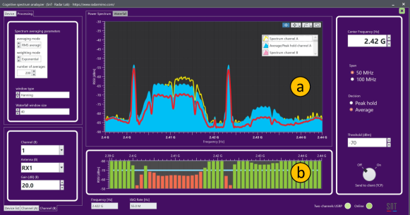
Figure 5: A snapshot of the developed two-channel Spectrum Sensing Application. (a) Power spectrum. (b) The energy detector.

II-C Cognitive MIMO Radar

The cognitive MIMO radar application was developed based on LabView NXG 3.1, and was connected to the HW platform NI-USRP 2944R. This USRP consists of a $2\times 2$ MIMO RF transceiver with a programmable Kintex-7 field programmable gate array (FPGA). The developed application is quite flexible in terms of changing the transmit waveform on the fly, such that it can adapt with the environment. TABLE II details the features and flexibilities of the developed application. The center frequency can be adjusted to any arbitrary value in the interval $70$ MHz to $6$ GHz, and the radar bandwidth can be adjusted to any arbitrary value in the interval $1$ MHz to $80$ MHz.

Further, up to two targets can be also emulated in this application. Passing the transmitting waveforms through the $30$ dB attenuators as indicated in Figure 4(b), a reflection will be generated; this will be used to generate the targets, contaminated with the communications interference. The received signal in this way will be further shifted in time, frequency and spatial direction to create the simulated targets. These targets will be detected after calculating the absolute values of the range-Doppler maps.

The block diagram of the developed cognitive MIMO radar is depicted in Figure 6. Note that the application is connected through a network (LAN/Wi-Fi) to the spectrum sensing application to receive the information about the occupied frequency bands. The radar adapts its transmit waveform and the matched filter coefficients based on this information. Then, using the two transmit channels of NI-USRP 2944R, the optimized MIMO waveforms will be transmitted; the design algorithm for the optimization is described in Section III.

Figure 7 depicts a snapshot of the developed cognitive MIMO radar application framework, when the licensed band $3.78$ GHz with $40$ MHz bandwidth was used for transmission. All the parameters related to the radar waveform, processing units, and targets can be changed and adjusted during the operation of the radar system.

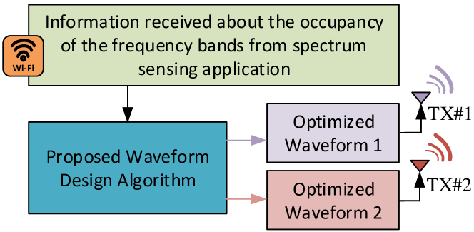
(a) Transmitter

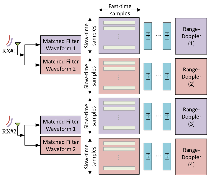
(b) Receiver

Figure 6: Block diagram of the developed cognitive MIMO radar application. In the transmit side (a), a list of occupied frequency bands will be received through the network connection between the spectrum sensing application and the radar application. Based on this information, the proposed design algorithm optimizes the transmitting waveforms. At the receive side (b), the optimized waveforms will be used for appropriate matched filtering in the fast-time dimension. Consequently, the modulus of the range-Doppler plots will be calculated after taking FFT in the slow-time dimension.

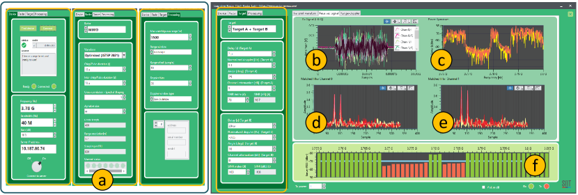
Figure 7: A snapshot of the developed cognitive MIMO radar application. (a) Settings for device, radar, and processing parameters. (b) I and Q signals of two receive channels. (c) Spectrum of the received signals in two receive channels. (d) Matched filters to two transmitting waveforms at the first receive channel. (e) Matched filters to two transmitting waveforms at the second receive channel. (f) Received information from the energy detector of the spectrum sensing application.

III Waveform Design

We consider a colocated narrow-band MIMO radar system, with $M$ transmit antennas, each transmitting a sequence of length $N$ in the fast-time domain. Let the matrix $\mbox{\boldmath{$X$}}\in\mathbb{C}^{M\times N}\triangleq[\mathbf{x}_{1}^{T},\dots,\mathbf{x}_{M}^{T}]^{T}$ denotes the transmitted set of sequences in baseband, where the vector $\mathbf{x}_{m}\triangleq[x_{m,1},\ldots,x_{m,N}]^{T}\in\mathbb{C}^{N}$ ($m=\{1,\dots,M\}$) indicates the $N$ samples of $m^{th}$ transmitter. We aim to design a transmit set of sequences which have small cross-correlation among each others, while each of the sequences having a desired spectral behaviour. To this end, in the following, we introduce the SILR and ICCL metrics and subsequently the optimization problem to handle them.

Let $\mbox{\boldmath{$F$}}\triangleq[\mathbf{f}_{0},\dots,\mathbf{f}_{N-1}]\in\mathbb{C}^{N\times N}$ be the Discrete Fourier Transform (DFT) matrix, where, $\mathbf{f}_{k}\triangleq[1,e^{j\frac{2\pi k}{N}},\dots,e^{j\frac{2\pi k(N-1)}{N}}]^{T}\in\mathbb{C}^{N},\ k=\{0,\dots,N-1\}$. Let $\mathcal{V}$ and $\mathcal{U}$ be the desired and undesired discrete frequency bands for MIMO radar, respectively. These two sets satisfy $\mathcal{V}\cup\mathcal{U}=\{0,\dots,N-1\}$ and $\mathcal{V}\cap\mathcal{U}=\emptyset$. We define SILR as,

$$g_{s}(\mbox{\boldmath{$X$}})\triangleq\frac{\sum_{m=1}^{M}\mathinner{\!\left\lVert\mathbf{f}_{k}^{\dagger}\mathbf{x}_{m}\right\rVert}^{2}|k\in\mathcal{U}}{\sum_{m=1}^{M}\mathinner{\!\left\lVert\mathbf{f}_{k}^{\dagger}\mathbf{x}_{m}\right\rVert}^{2}|k\in\mathcal{V}}$$ (2)

which is the energy of the radar waveform interfering with other incumbent services (like communications) relative to the energy of transmission in the desired bands. Optimizing the above objective function may shape the spectral-power of the transmitting sequence and satisfy a desired mask in the spectrum. However, in a MIMO radar it is necessary to separate the transmitting waveforms in the receiver to investigate the waveform diversity, which ideally requires orthogonality between the transmitting sequences. To make this orthogonality feasible by CDM, we need to transmit a set of sequences which have small cross-correlations among each other. The aperiodic cross-correlation of $\mathbf{x}_{m}$ and $\mathbf{x}_{l}$ is defined as, $r_{m,m^{\prime}}(l)=\sum_{n=1}^{N-l}x_{m,n}x_{m^{\prime},n+l}^{*}$, where $m\neq m^{\prime}\in\{1,\dots,M\}$ are indices of the transmit antennas and $l\in\{-N+1,\dots,N-1\}$ denotes the cross-correlation lag. We define ICCL as,

$$\widetilde{g}_{c}(\mbox{\boldmath{$X$}})\triangleq\sum_{m=1}^{M}\sum_{\begin{subarray}{c}{m^{\prime}=1}\\ {m^{\prime}\neq m}\end{subarray}}^{M}\sum_{l=-N+1}^{N-1}|r_{m,m^{\prime}}(l)|^{2},$$ (3)

which can be used to promote the orthogonality between the transmitting sequence.

III-A Problem Formulation

We aim to design sets of sequences that simultaneously have good properties in terms of SILR and ICCL, under constant modulus and discrete phase constraints. The optimization problem can be represented as,

$$\begin{dcases}\min_{\mbox{\boldmath{$X$}}}&g_{s}(\mbox{\boldmath{$X$}}),g_{c}(\mbox{\boldmath{$X$}})\\ s.t&C_{1}\ \text{or}\ C_{2}\end{dcases}$$ (4)

where $g_{c}(\mbox{\boldmath{$X$}})=\frac{1}{(2MN)^{2}}\widetilde{g}_{c}(\mbox{\boldmath{$X$}})$ is the scaled version of the ICCL as defined in (3). Further, $C_{1}\triangleq\{\mbox{\boldmath{$X$}}\mid x_{m,n}=e^{j\phi_{m,n}},\phi_{m,n}\in\Omega_{\infty}\},\Omega_{\infty}=[0,2\pi)$ is the constant modulus constraint and $C_{2}\triangleq\{\mbox{\boldmath{$X$}}\mid x_{m,n}=e^{j\phi_{m,n}},\phi_{m,n}\in\Omega_{L}\},\Omega_{L}=\left\{0,\frac{2\pi}{L},\dots,\frac{2\pi(L-1)}{L}\right\}$ is discrete phase constraint. In fact, $\Omega_{L}$ indicates the $M$-ary Phase Shift Keying (MPSK) with alphabet size $L$.

Problem (4) is a bi-objective optimization problem in which a feasible solution that minimizes the both the objective functions may not exist [52, 59]. Scalarization is a well known technique that converts the bi-objective optimization problem to a single objective problem by replacing a weighted sum of the objective functions. Using this technique, the following Pareto-optimization problem will be obtained,

$$\mathcal{P}\begin{dcases}\min_{\mbox{\boldmath{$X$}}}&g(\mbox{\boldmath{$X$}})\triangleq\theta g_{s}(\mbox{\boldmath{$X$}})+(1-\theta)g_{c}(\mbox{\boldmath{$X$}})\\ s.t&C_{1}\ \text{or}\ C_{2},\end{dcases}$$ (5)

The coefficient $\theta\in\left[0,1\right]$ is a weight factor that effects trade-off between SILR and ICCL. In (5), $g_{s}(\mbox{\boldmath{$X$}})$ is a fractional quadratic function while $g_{c}(\mbox{\boldmath{$X$}})$ is quartic function, both with multiple variables. Further, both $C_{1}$ and $C_{2}$ constraints are not an affine set, besides $C_{2}$ is non-continuous and non-differentiate set. Therefore, we encounter a non-convex, multi-variable and NP-hard optimization problem [52, 60].

III-B The Proposed Method

To solve (5) directly, we utilize the CD framework wherein the multi variable problem is solved as a sequence of single variable problems. The methodologies based on CD, generally start with a feasible matrix $\mbox{\boldmath{$X$}}=\mbox{\boldmath{$X$}}^{(0)}$ as the initial waveform set. Then, in each iteration, the waveform set is updated entry by entry several times [61]. In particular, an entry of $X$ is considered as the only variable while others are held fixed and then the objective function is optimized with respect to this identified variable. Let us assume that $x_{t,d}$ ($t\in\{1,\dots,M\}$ and $d\in\{1,\dots,N\}$) is the only variable and the fixed entries are stored in the matrix $\mbox{\boldmath{$X$}}_{-(t,d)}^{(i)}$. The resulting single-variable objective function at $(i)^{th}$ iteration can be written as (see Appendix A),

$$g(x_{t,d},\mbox{\boldmath{$X$}}_{-(t,d)}^{(i)})= \theta\frac{a_{0}x_{t,d}+a_{1}+a_{2}x_{t,d}^{*}}{b_{0}x_{t,d}+b_{1}+b_{2}x_{t,d}^{*}}$$ (6)

$$+ (1-\theta)\left(c_{0}x_{t,d}+c_{1}+c_{2}x_{t,d}^{*}\right)$$

where, the coefficients $a_{i}$, $b_{i}$ and $c_{i}$ depend on $\mbox{\boldmath{$X$}}^{(i)}_{-(t,d)}$ and are derived in Appendix A. By substituting $x_{t,d}=e^{j\phi}$, $\mathcal{P}$ in (5) the optimization problem at the $i^{th}$ iteration can be recast as a function of $\phi$ as follows,

$$\begin{dcases}\min_{\phi}&\theta\frac{a_{0}e^{j\phi}+a_{1}+a_{2}e^{-j\phi}}{b_{0}e^{j\phi}+b_{1}+b_{2}e^{-j\phi}}+(1-\theta)\left(c_{0}e^{j\phi}+c_{1}+c_{2}e^{-j\phi}\right)\\ s.t&C_{1}\ \text{or}\ C_{2},\end{dcases}$$ (7)

At the $i^{th}$ iteration, for $t=1,\ldots,M$, and $d=1,\ldots,N$, the $(t,d)^{th}$ entry of $X$ will be updated by solving (7). After updating all the entries, a new iteration will be started, provided that the stopping criteria is not met. This procedure will continue until the objective function converges to an optimal value. A summary of the proposed method is reported in Algorithm 1.

Input: Initial set of feasible sequences, $\mbox{\boldmath{$X$}}^{(0)}$.

Initialization: $i\mathrel{\mathop{\ordinarycolon}}=0$.

Optimization:

1. while the stopping criteria is not met, do

2. $i\mathrel{\mathop{\ordinarycolon}}=i+1$;

3. for $t=1,\dots,M$ do

4. for $d=1,\dots,N$ do

5. Optimize $x_{t,d}^{(i-1)}$ and obtain $x^{\star}_{t,d}$;

6. Update $x^{(i)}_{t,d}=e^{j\phi^{\star}}$;

7. $\mbox{\boldmath{$X$}}^{(i)}=\mbox{\boldmath{$X$}}^{(i)}_{-(t,d)}|_{x_{t,d}=x^{(i)}_{t,d}}$;

8. end for

9. end for

10. end while

Output: $\mbox{\boldmath{$X$}}^{\star}=\mbox{\boldmath{$X$}}^{(i)}$.

Algorithm 1 The proposed method for designing set of sequences that avoid reserved frequency bands, and in a same time have small cross-correlation among each other.

Let $\phi^{\star}$ be the optimized solution of Problem (7). Algorithm 1 considers a feasible set of sequences as the initial waveforms. Then, at each single variable update, it selects $x_{t,d}^{(i-1)}$ as the variable and updates it with the optimized ${s_{t,d}^{(i)}}$, denoted by ${s_{t,d}^{\star}}$. This procedure is repeated for other entries and is undertaken until all the entries are optimized at least once. After optimizing the $MN^{th}$ entry, the algorithm examines that the waveform converges to a stationary point. If the stopping criteria is not met the algorithm repeats the aforementioned steps. The solution to the single variable optimization problem $\mathcal{P}^{(i)}$ can be obtained by following similar steps of the proposed method in [54], where the the key steps are detailed in the following.

III-B1 Continuous phase constraint

The solution under continuous phase will be obtained by finding the critical points of the objective function and selecting the one that minimizes the objective. This is omitted for brevity.

III-B2 Discrete phase constraint

In this case, the feasible set is limited to a set of $L$ phases. Thus, the objective function with respect to the indices of $\Omega_{L}$ can be written as,

$$g(l)=\theta\frac{\sum_{n=0}^{2}a_{n}e^{-j\frac{2\pi nl}{L}}}{\sum_{n=0}^{2}b_{n}e^{-j\frac{2\pi nl}{L}}}+(1-\theta)e^{\frac{j2\pi l}{L}}\sum_{n=0}^{2}c_{n}e^{-j\frac{2\pi nl}{L}}$$ (8)

where, $l=\{0,\dots,L-1\}$. The summation term in the numerator and denominator in Equation (8) is exactly the definition of $L-$point DFT of sequences $[a_{0},a_{1},a_{2}]$ , $[b_{0},b_{1},b_{2}]$ and $[b_{0},b_{1},b_{2}]$ respectively. Therefore, $g(l)$ can be written as,

$$g(l)=\theta\frac{\mathcal{F}_{L}\{a_{0},a_{1},a_{2}\}}{\mathcal{F}_{L}\{b_{0},b_{1},b_{2}\}}+(1-\theta)\mbox{\boldmath{$h$}}\odot\mathcal{F}_{L}\{c_{0},c_{1},c_{2}\}.$$ (9)

where, $\mbox{\boldmath{$h$}}=[1,e^{-j\frac{2\pi}{L}},\ldots,e^{-j\frac{2\pi(L-1)}{L}}]^{T}\in\mathbb{C}^{L}$ and $\mathcal{F}_{L}$ is $L-$point DFT operator. The current function is valid only for $L>2$. According to periodic property of DFT, for binary $g(l)$ can be written as,

$$g(l)=\theta\frac{\mathcal{F}_{L}\{a_{0}+a_{2},a_{1}\}}{\mathcal{F}_{L}\{b_{0}+b_{2},b_{1}\}}+(1-\theta)\mbox{\boldmath{$h$}}\odot\mathcal{F}_{L}\{c_{0}+c_{2},c_{1}\}.$$ (10)

Finally ${l^{\star}}=\arg\displaystyle{\min_{l=1,\dots,L}}\left\{g(l)\right\}$, and ${\phi_{d}^{\star}}=\frac{2\pi({l^{\star}}-1)}{L}.$

IV Performance Analysis

This section deals with a simulation framework to compare the performance of the proposed method in terms of SILR and ICCL with the counterparts. To terminate Algorithm 1, we consider $\Delta\mbox{\boldmath{$X$}}^{(i)}\triangleq\mathinner{\!\left\lVert\mbox{\boldmath{$X$}}^{(i)}-\mbox{\boldmath{$X$}}^{(i-1)}\right\rVert}_{F}\leq\zeta$ as the stopping criterion, and set $\zeta=10^{-5}$ for all the ensuing examples. Let $\mathcal{S}=\cup_{k=1}^{K_{s}}(s_{k,1},s_{k,2})$ be the $K_{s}$ number of normalized frequency stop bands, where $0\leq s_{k,1}<s_{k,2}\leq 1$ and $\cap_{k=1}^{K_{s}}(s_{k,1},s_{k,2})=\emptyset$. Thus, the undesired discrete frequency band is given by, $\mathcal{U}=\cup_{k=1}^{K_{s}}(\lfloor Ns_{k,1}\rceil,\lfloor Ns_{k,2}\rceil)$.

Figure 8(a) shows the convergence behavior of the objective function of the proposed method under $C_{1}$ and $C_{2}$ constraints for different values of $\theta$. Algorithm 1 was initialized using random-phase sequences and identical initial sequences was used for all the counterparts in case of any comparison. As can be seen, the objective function decreases monotonically and converges to a certain value under both $C_{1}$ and $C_{2}$ constraints. In case of the $C_{1}$ constraint, a better performance can be observed due to the higher degrees of freedom in comparison to the $C_{2}$ constraint. Further, Figure 8(b) numerically shows the convergence of the argument to the stationary points ($\Delta\mbox{\boldmath{$X$}}^{(i)}$) for different values of $\theta$.

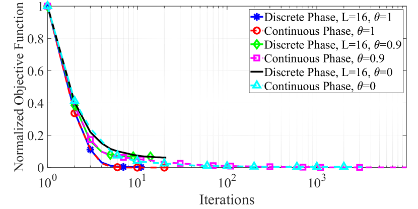
(a) Objective function.

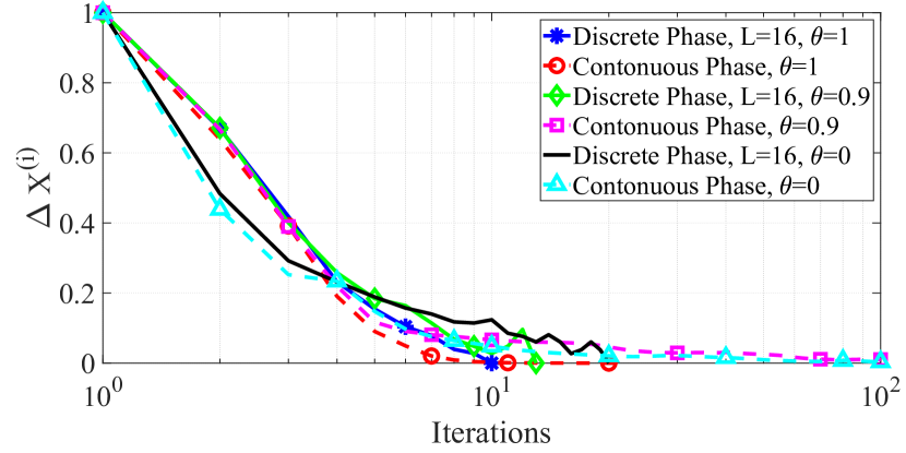
(b) $\Delta\mbox{\boldmath{$X$}}^{(i)}$.

Figure 8: Convergence behavior of the proposed method under continuous and discrete phase constraints for different $\theta$ values ($M=4$, $N=64$ and $L=16$).

In Figure 9, we set $\theta=1$ to design a set of sequences optimized based on SILR minimization. We set $M=3$, and denote the spectral behaviour of the optimized sequence of $m^{th}$ transmitter as $\mbox{\boldmath{$x$}}_{m}$ in Figure 9. The figure shows that the spectral behaviour of the optimized waveforms obtained by the proposed method provide deeper notches under $C_{1}$ constraint, when compared with SHAPE [26] under a similar constraint. Under the $C_{2}$ constraint, the proposed algorithm outperforms the Spectrum Discrete Phase Modulation (SDPM) [42], indicating the effectiveness of the proposed method over the counterparts in shaping the spectrum of the waveforms.

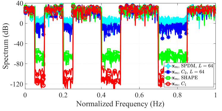
Figure 9: Comparing the performance of the proposed method ($\theta=1$) with SHAPE [26] and SDPM [42] in case of spectral shaping ($M=3$, $m=\{1,2,3\}$, $N=512$, $L=64$ and $\mathcal{S}=[0.05,0.1]$ $\cup[0.2,0.25]$ $\cup[0.4,0.5]$ $\cup[0.7,0.85]$ Hz). All the methods are initialized with the same set of random-phase sequences with $L=64$.

Next, we set $\theta=0$ and evaluate the performance of the proposed method in terms of ICCL minimization. In this case, we consider Multi-CAN [45] and Binary Sequences seTs (BiST) [52] (preforming ISL minimization) as the benchmarks to compare the performance under $C_{1}$ and $C_{2}$ constraints. Figure 10(a) compares the cross-correlation of the first and second optimized waveforms obtained by the proposed method, Multi-CAN and BiST algorithms, for $N=64$ and $M=3$. Intuitively, it can be seen that the proposed method offers set of sequences with smaller cross-correlation levels. In Figure 10(b) and Figure 10(c), we fix $M=3$ and evaluate the ICCL of the waveforms obtained by the proposed method by changing the sequence length, and vice versa, fixing $N=64$ and changing number of transmitting waveforms. In both cases, we compare the performance of the proposed method with Multi-CAN and BiST. It can be observed from this figure that the proposed method obtains smaller ICCL in compare with the counterparts.

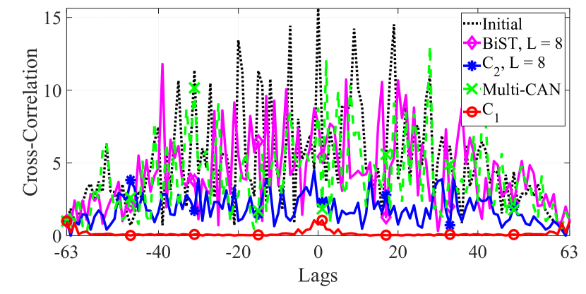
(a) $M=3$, and $N=64$.

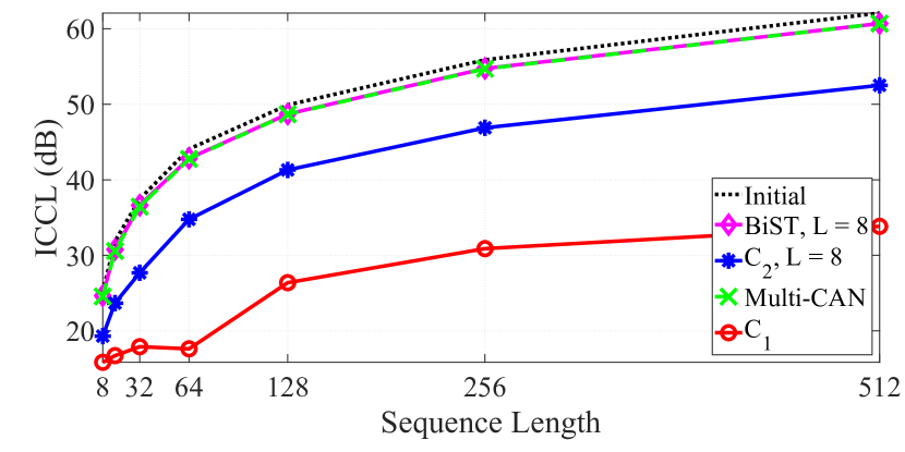
(b) $M=3$.

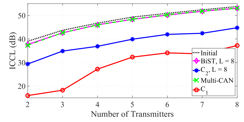
(c) $N=64$.

Figure 10: Comparing the performance of the proposed method ($\theta=0$) with Multi-CAN [45] and BiST [52] in terms of ICCL. All the methods are initialized with the same set of random-phase sequences.

In Figure 11, we evaluate the trade-off between a good spectrum shaping and good orthogonality by choosing $\theta$. Figure 11(a) shows the impact of $\theta$ on the spectral behaviour. As can be seen, by choosing $\theta=0$, the optimized waveforms are not able to put notches on the undesired frequencies. By increasing $\theta$, the notches will appear gradually and in case of $\theta=1$, we obtain the deepest notches. However, when $\theta=1$ the cross-correlation is at the highest level which decreases with $\theta$. In $\theta=0$, we obtain the best orthogonality. This fact is shown in Figure 11(b). Therefore, by choosing an appropriate value of $\theta$, one can make a good trade-off between these two metrics. For instance, choosing $\theta=0.75$ is able to put a null level around $50$ dB (see Figure 11(a)), while having good cross-correlation level (see Figure 11(b)).

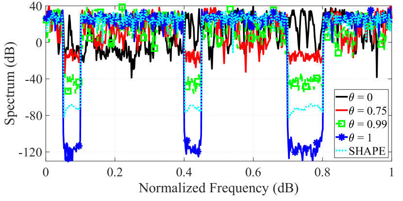
(a) Spectrum of the proposed method for different $\theta$ values ($\mathcal{S}=[0.05,0.1]$ $\cup[0.4,0.45]$ $\cup[0.7,0.8]$ Hz).

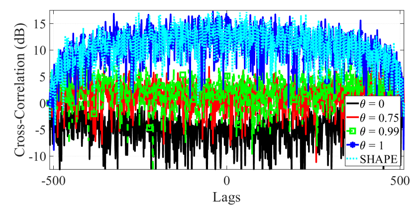
(b) Cross-Correlation of the proposed method for different $\theta$ values.

Figure 11: The impact of $\theta$ value on trade-off between (a) spectral shaping and (b) cross-correlation levels in comparision with SHAPE [26] ($M=2$ and $N=512$).

V Experiments and Results

In this section, we present present experiments conducted using the developed prototype and analyze the HW results. The prototype setup in Figure 4(a) depicts the cognitive MIMO radar, the spectrum sensing application and the LTE application framework as well as RF cable enclosure, USRP s, and the spectrum analyzer. For the practical applicability of our methods and verification of the simulation, we established all the connections shown in Figure 4(b) using RF cables and splitters/ combiners, and measured the performance in a controlled environment. Nevertheless, a video of the OTA operation of the proposed prototype can be found in radarmimo.com.

The developed cognitive MIMO radar system in the proposed coexistence prototype consists of a $2\times 2$ transmit/receive unit. Two targets with adjustable attenuation paths, Doppler and spatial angles can be also augmented in the receive side as described in Section II. The transmitting waveforms can be selected based on the options in TABLE II or obtained based on Algorithm 1. When executing the application, input parameters to optimize the waveforms pass from the Graphical User Interface (GUI) to MATLAB, and the optimized set of sequences are passed to the application through the GUI. The other processing blocks of the radar system including matched filtering, Doppler processing, and scene generation are developed in the LabView G dataflow application. TABLE III and TABLE IV summarize the parameters used for radar and targets in this experiment.

TABLE III: Radar experiment parameters

Parameters	Value
Center frequency	$2$ GHz
Real-time bandwidth	$40$MHz
Transmit and receive channels	$2\times 2$
Transmit power	$10$ dBm
Duty cycle	$50\%$
Transmit code length	$400$
Pulse repetition interval	$20\mu$s

TABLE IV: Target experiment parameters

Parameters	Target 1	Target 2
Range delay	$2\mu$s	$2.6\mu$s
Normalized Doppler	$0.2$ Hz	$-0.25$ Hz
Angle	$25\deg$	$15\deg$
Attenuation	$30$ dB	$35$ dB

For the LTE communications, we established the downlink between a BS and one user. Nonetheless, the experiments can be also be performed with uplink LTE as well as bi-directional LTE link. LabVIEW LTE framework offers the possibility to vary the Modulation and Coding Schemes (MCS) of PDSCH from $0$ to $28$ where the constellation size goes from QPSK to $64$QAM [62]. LTE uses PDSCH for the transport of data between the BS and the user. TABLE V indicates the experimental parameters used in our test set-up for the communications.

TABLE V: Communications experiment parameters

Parameters	Value
Communication MCS	MCS0 (QPSK $0.12$) MCS10 (16QAM $0.33$) MCS17 (64QAM $0.43$)
Center frequency (Tx and Rx)	$2$ GHz
Bandwidth	$20$ MHz

V-A Impact of SILR Minimization

In this experiment, we show the impact of SILR enhancement on the coexistence. We use the experiment parameters reported in TABLE III and TABLE V for radar and communications, respectively.

According to these tables, we utilize the radar with a $50\%$ duty cycle. By transmitting a set of $M=2$ waveforms with length $N=400$, radar transmissions will occupy a bandwidth of $40$ MHz. On the other side, the LTE communications framework utilizes $20$ MHz bandwidth for transmission. Further, we select the allocation $1111111111110000000111111$ for the LTE resource block ($4$ physical resource blocks/bit), where the entry “1” indicates the use of the corresponding time-bandwidth resources in the LTE application framework. The spectrum of this LTE downlink is measured with the developed spectrum sensing application as depicted in Figure 12(a). By setting $\theta=1$ in (5), the radar optimizes its transmit waveform to avoid interference with the bands occupied by the LTE resource blocks, while exploiting the holes in the $20$ MHz of the LTE spectrum. A screen capture of the resulting spectrum occupied by radar and communications is depicted in Figure 12. This figure serves two purposes, (i) focusing on the LTE downlink spectrum, it validates the spectrum analyzer application with a commercial product, and (ii) it clearly indicates that the desired objective of spectrum shaping is met. The impact of this matching on performance of radar and communications are presented next.

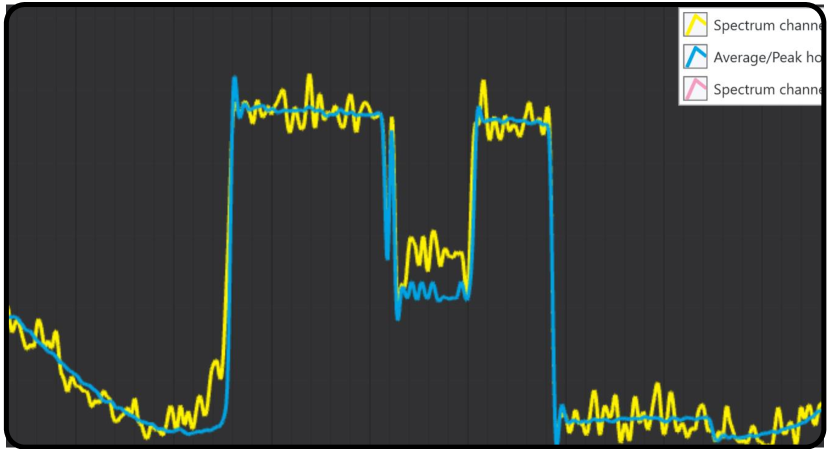
(a) LTE at developed application.

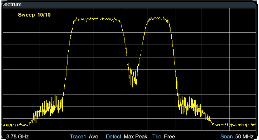
(b) LTE at R&H spectrum analyzer.

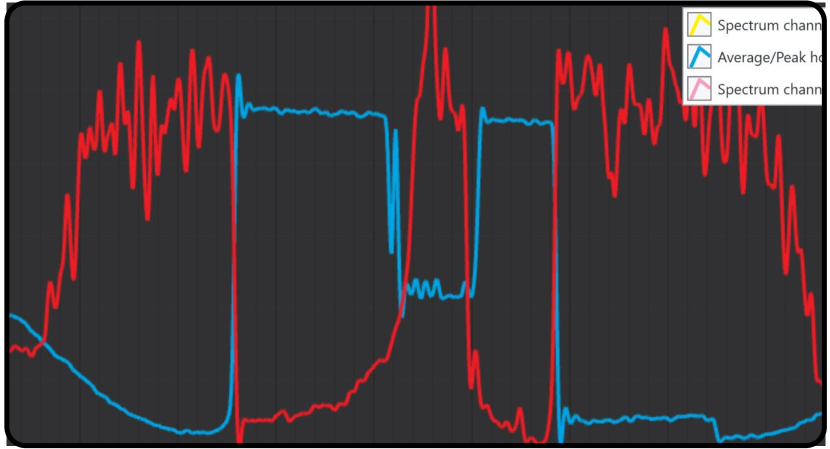
(c) Radar and LTE at developed application.

Figure 12: Screen captures of the resulting spectrum occupied by the LTE communications and radar signals at the developed two-channel spectrum sensing application and R&H spectrum analyzer. The spectrum of the LTE downlink in (a) is validated by a commercial product in (b), and (c) indicates the the resulting spectrum of both communications (blue) and radar (red) at the developed two-channel spectrum sensing application.

When the radar transmits random-phase sequences, it utilizes the entire bandwidth and the two system mutually interfere. In fact, the operations of both radar and communications are disrupted as depicted in Figure 13 (a and c), thereby creating difficulties for their coexistence. In this case, by utilizing the SILR optimized waveforms obtained by setting $\theta=1$ in Algorithm 1, the performance of both systems are enhanced as indicated pictorially in Figure 13 (b and d). A possible short-coming is the potentially higher cross-correlation levels of the two transmit waveforms leading to false targets impacting the radar performance.

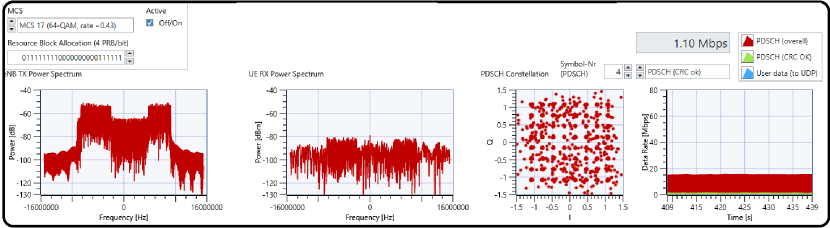
(a) Random-phase sequences.

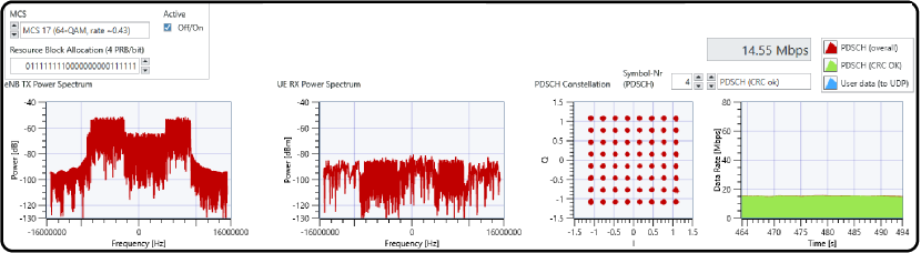
(b) Optimized sequences ($\theta=1$).

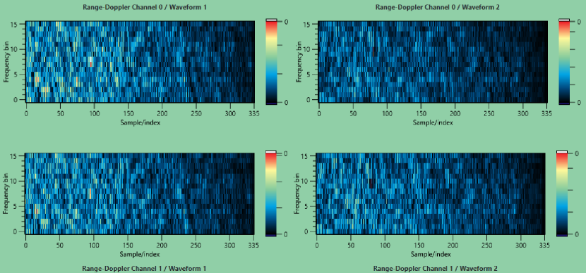
(c) Random-phase sequences.

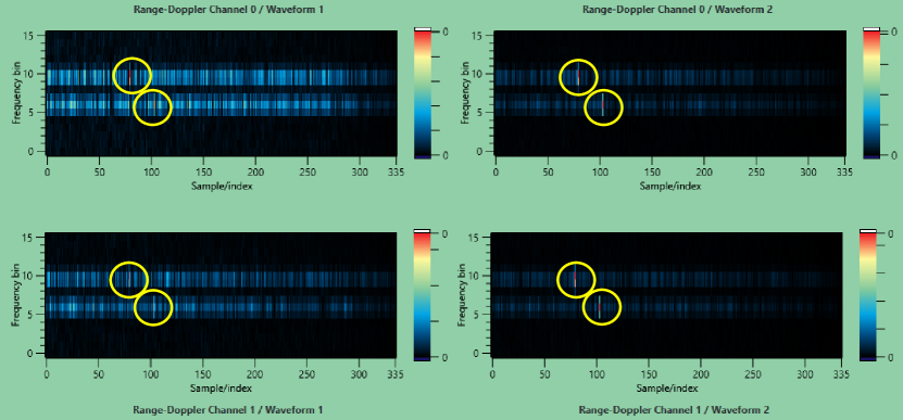
(d) Optimized sequences ($\theta=1$).

Figure 13: LTE application framework in the presence of radar signal. In case of transmitting random-phase sequences in radar at the same frequency band of communications, the throughput of communications decreases drastically which is depicted in (a). In this case, radar also cannot detect targets as depicted in (c). In case of transmitting the optimized waveforms, the performance of both radar and communications enhances (b and c).

V-B ICCL Minimization

In the absence of the LTE downlink, the radar can optimize its waveform based on ICCL minimization by setting $\theta=0$ in Algorithm 1. Figure 14 indicates the performance of the radar system in this case in comparison with a set of random-phase sequences. The lower cross-correlation of the optimized sequences can be visually observed from the lack of sidelobes in this figure. Since the SILR is not considered, this optimized sequence is observed to occupy the entire band causing degradation to communication link.

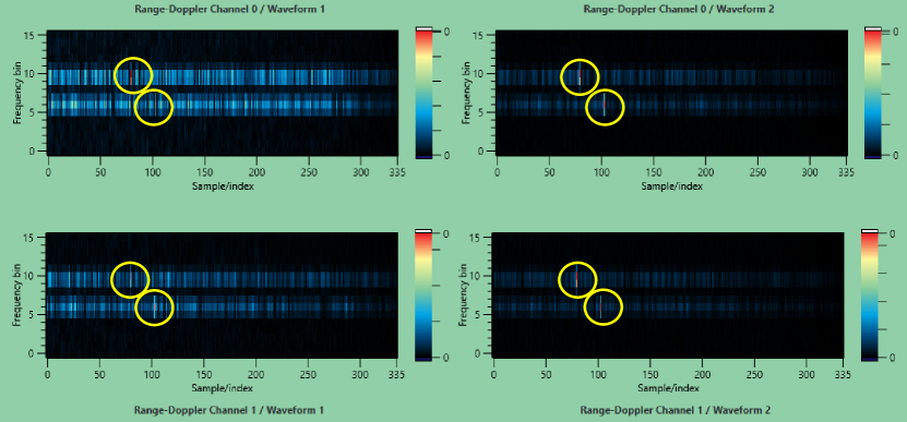
(a) Random-phase sequences.

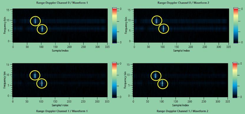
(b) Optimized waveforms ($\theta=0$).

Figure 14: Range-Doppler plots for random-phase and optimized sequences obtained by Algorithm 1 with $\theta=0$.

V-C Trade-off between SILR and ICCL

This section evaluates the performance of the optimized waveforms when $\theta=0.75$, a value shown in Section IV to offer an adequate trade-off between spectrum shaping and low cross-correlation. We first evaluate the performance of radar and communication experiencing mutual interference when the radar does not undertake the waveform optimization. Subsequently, we let the radar optimize its waveform by setting $\theta=0.75$. Figure 15 depicts range-Doppler plots of this case.

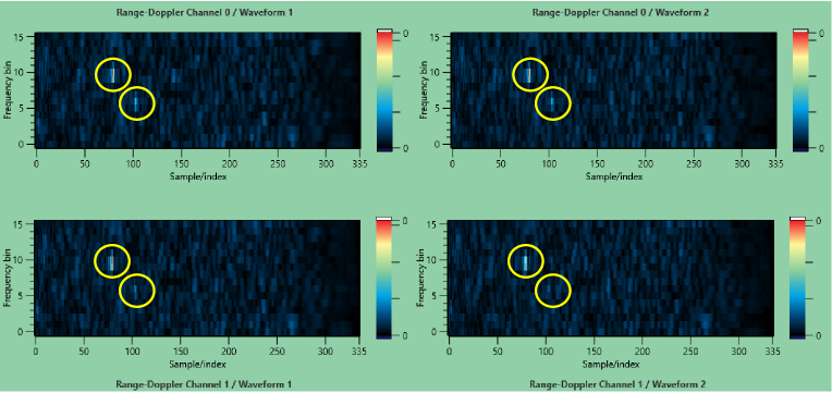
Figure 15: The performance of the radar in case of transmitting optimized waveforms with $\theta=0.75$.

To evaluate the corresponding performances, we calculate the SINR of the two targets for radar while on the communication side, report the PDSCH throughput calculated by the LTE application framework. We perform our experiments in following steps:

• Step-1: In the absence of radar transmission, we collect the LTE PDSCH throughput for MCS0, MCS10 and MCS 17. For each MCS, we use LTE transmit power of $5$ dBm, $10$ dBm, $15$ dBm and $20$ dBm.

• Step-2: In the absence of LTE transmission, we obtain the received Signal to Noise Ratio (SNR) for the two targets. The SNR is calculated as the ratio of the peak power of the detected targets to the average power of the cells close to the target location in the range-Doppler map.

• Step-3: We transmit a set of random-phase sequences as the radar waveform. At the same time, we transmit the LTE waveform and let the two waveforms interfere with each other. We log the PDSCH throughput as well as the SINR of Target-$1$ and Target-$2$. We perform this experiment for MCS0, MCS10 and MCS17 and for each MCS, we increase the LTE transmit power from $5$ dBm to $20$ dBm in steps of $5$ dBm. Throughout the experiment we keep the radar transmit power fixed. For each LTE MCS and LTE transmit power combination, we average over $5$ experiments before logging the PDSCH throughput and target SINR s.

• Step-4: We repeat step-3, but using the optimized waveforms with $\theta=0.75$ at the radar transmitter. This optimization is carried out in real-time as mentioned earlier using the spectrum sensing application and the Algorithm 1 implementation.

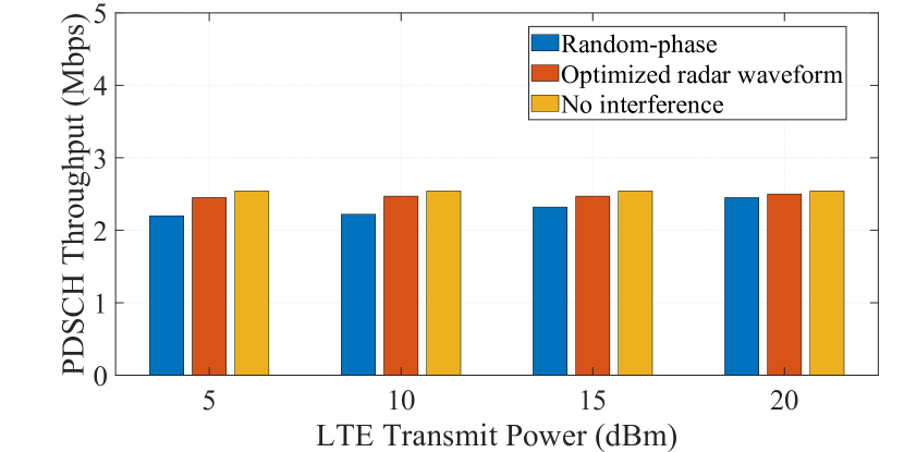
(a) MCS 0 (QPSK $0.12$)

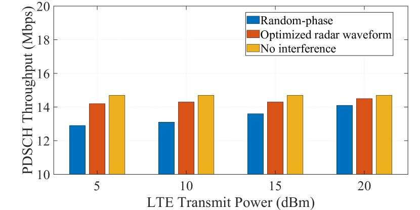
(b) MCS 10 (16QAM $0.33$)

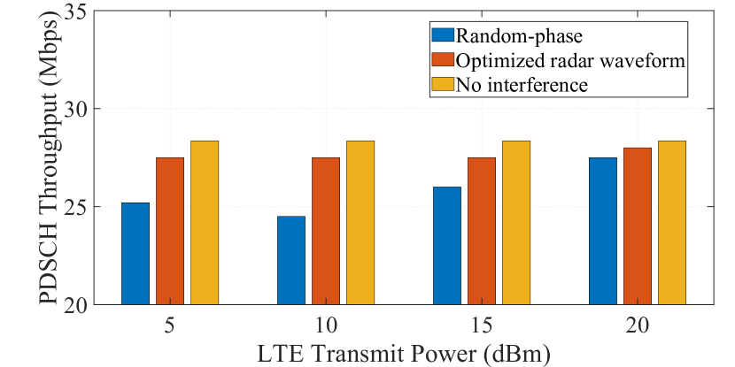
(c) MCS 17 (64QAM $0.43$)

Figure 16: PDSCH throughput of LTE under radar interference. We observe that with radar interference reduces the PDSCH throughput but with cognitive spectrum sensing followed by spectral shaping of the radar waveform PDSCH throughput improves for all the LTE MCS.

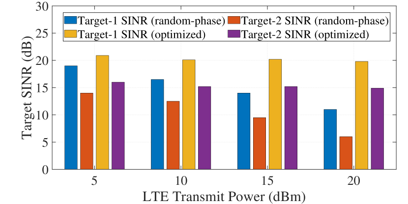
(a) MCS 0 (QPSK $0.12$)

(b) MCS 10 (16QAM $0.33$)

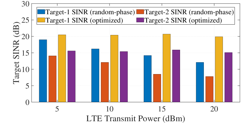
(c) MCS 17 (64QAM $0.43$)

Figure 17: SINR of targets under interference from donwlink LTE link. We observe that by optimizing the transmitting waveforms, the SNR of both the targets improves. Note that in this experiment the SNR upper-bound for the first and the second target in the absence of communications interference was $22$ dB, and $17$ dB, respectively.

The performance of the communication link in terms of PDSCH throughput is shown in Figure 16. We first observe that, the throughput of the link degrades in the presence of radar interference. The degradation becomes prominent at higher MCS since the SINR requirement to obtain a clean constellation for larger modulations is also high. Subsequently, when the radar optimizes its waveform as per Algorithm 1, the LTE throughput improves. Again we see that the improvement is prominent in the higher MCS. This is due to the fact that after a certain SINR, the lower MCS do not show any symbol error as the constellation points are already well separated. But as the distance between the constellation points decrease, even a small improvement of SINR leads to improved Error Vector Magnitude (EVM) which leads to improved decoding and hence a prominent increase in throughput.

We set $\theta=0.75$, such that the optimized waveforms avoid the frequency bands occupied by communications, and simultaneously have an acceptable cross-correlation. In this case, the performance of the radar in terms of target SNR is shown in Figure 17. In the presence of LTE interference, we observe that the SINR s of Target-1 and Target-2 degrade. These quantities improve when the radar optimizes the transmitting waveforms. Interestingly, when the LTE transmission power is high ($15$ dBm, and $20$ dBm), higher improvement results from the avoidance of the used LTE bands. Precisely, when the communication system is transmitting with a power of $20$ dBm, use of the optimized waveforms enhances the SINR of Target-1, and Target-2 in excess of $7$ dB in all the MCS values. Note that, due to the different attenuation paths that is considered for the two targets (see TABLE III ), the measured SINR s for these targets are different. Also, in the absence of the LTE interference, the achieved SINR of Target-1, and Target-2 is $22$ dB and $17$ dB, respectively, which is the upper bound for the achievable SINR through the optimized waveforms in presence of the communications interference.

VI Conclusion

In this paper, a radar-centric approach has been pursued towards a coexistence with communication systems. Particularly, the paper developed a SDR based cognitive MIMO radar prototype using USRP devices that coexist with LTE links. To enable seamless operation of incumbent LTE links and opportunistic radar sensing, the paper relied on cognition achieved through the implementation of a spectrum sensing followed by the development of a MIMO waveform design process. An algorithm based on CD approach is considered to design a set of sequences, where the optimization is based on real-time feedback received from the environment through the spectrum sensing application. The developed prototype is tested both in controlled environment and OTA to validate its functionalities and the experimental results indicating adherence to system requirements and performance enhancement are noted. A further development of this first coexistence prototype can be spatial beamforming in addition to the spectral shaping that can be considered in advanced cognitive MIMO radar systems.

Appendix A

SILR coefficients

Let $g_{a}(\mbox{\boldmath{$X$}})$ and $g_{b}(\mbox{\boldmath{$X$}})$ be the numerator and denominator of $g_{s}(\mbox{\boldmath{$X$}})$ respectively. Therefore $g_{a}(\mbox{\boldmath{$X$}})$ can be written as,

$$g_{a}(\mbox{\boldmath{$X$}})\triangleq \textstyle\sum_{m=1}^{M}\mathinner{\!\left\lVert\mathbf{f}_{k}^{\dagger}\mathbf{x}_{m}\right\rVert}^{2}|k\in\mathcal{U}=\sum_{m=1}^{M}\sum_{k\in\mathcal{U}}\mathbf{x}_{m}^{\dagger}\mathbf{f}_{k}\mathbf{f}_{k}^{\dagger}\mathbf{x}_{m}$$ (11)

$$= \textstyle\sum_{m=1}^{M}\mathbf{x}_{m}^{\dagger}\mbox{\boldmath{$F$}}_{\mathcal{U}}\mathbf{x}_{m}=\sum_{m=1}^{M}\sum_{n=1}^{N}\sum_{l=1}^{N}x_{m,n}^{*}u_{n,l}x_{m,l}$$

where, $\mbox{\boldmath{$F$}}_{\mathcal{U}}\triangleq\sum_{k\in\mathcal{U}}\mathbf{f}_{k}\mathbf{f}_{k}^{\dagger}\in\mathbb{C}^{N\times N}$ and $u_{n,l}$ are the elements of matrix $\mbox{\boldmath{$F$}}_{\mathcal{U}}$. By some mathematical manipulation it can be shown that, $g_{a}(\mbox{\boldmath{$X$}})=a_{0}x_{t,d}+a_{1}+a_{2}x_{t,d}^{*}$, where,

$$a_{0} \triangleq\textstyle\sum_{\begin{subarray}{c}{n=1}\\ {n\neq d}\end{subarray}}^{N}x^{*}_{t,n}u_{n,d},\ a_{2}\triangleq a_{0}^{*},$$ (12)

$$a_{1} \triangleq\textstyle\sum_{\begin{subarray}{c}{n=1}\\ {n\neq d}\end{subarray}}^{N}\sum_{{n,l=1}}^{N}x^{*}_{m,n}u_{n,l}x_{m,l}+\sum_{\begin{subarray}{c}{n,l=1}\\ {n,l\neq d}\end{subarray}}^{N}x^{*}_{t,n}u_{n,l}x_{t,l}+u_{d,d}.$$

Let us assume that, $\mbox{\boldmath{$F$}}_{\mathcal{V}}\triangleq\sum_{k\in\mathcal{V}}\mathbf{f}_{k}\mathbf{f}_{k}^{\dagger}\in\mathbb{C}^{N\times N}$. Likewise, $g_{b}(\mbox{\boldmath{$X$}})=b_{0}x_{t,d}+b_{1}+b_{2}x_{t,d}^{*}$, where $b_{i}$’s are obtained similar to $a_{i}$ with $v_{n,d}$, $v_{n,l}$ and $v_{d,d}$ replacing $u_{n,d}$, $u_{n,l}$ and $u_{d,d}$ respectively, and $v_{n,l}$ are the elements of matrix $\mbox{\boldmath{$F$}}_{\mathcal{V}}$.

ICCL coefficients

The ICCL can be written as, $\tilde{g}_{c}(\mbox{\boldmath{$X$}})=\sum_{\begin{subarray}{c}{m=1}\\ {m\neq t}\end{subarray}}^{M}\sum_{\begin{subarray}{c}{m^{\prime}=1}\\ {m^{\prime}\neq m,t}\end{subarray}}^{M}\sum_{k=-N+1}^{N-1}|r_{m,m^{\prime}}(l)|^{2}+\sum_{\begin{subarray}{c}{m^{\prime}=1}\\ {m^{\prime}\neq t}\end{subarray}}^{M}\sum_{l=-N+1}^{N-1}|r_{t,m^{\prime}}(l)|^{2}+\sum_{\begin{subarray}{c}{m=1}\\ {m\neq t}\end{subarray}}^{M}\sum_{l=-N+1}^{N-1}|r_{m,t}(l)|^{2}$. Since $\mathinner{\!\left\lVert r_{t,m}(l)\right\rVert}_{2}^{2}=\mathinner{\!\left\lVert r_{m,t}(l)\right\rVert}_{2}^{2}$, hence, $\tilde{g}_{c}(\mbox{\boldmath{$X$}})$ becomes,

$$\tilde{g}_{c}(\mbox{\boldmath{$X$}})=\gamma_{t}+2\textstyle\sum_{\begin{subarray}{c}{m=1}\\ {m\neq t}\end{subarray}}^{M}\sum_{l=-N+1}^{N-1}|r_{m,t}(l)|^{2}$$ (13)

where, $\gamma_{t}\triangleq\sum_{\begin{subarray}{c}{m=1}\\ {m\neq t}\end{subarray}}^{M}\sum_{\begin{subarray}{c}{m^{\prime}=1}\\ {m^{\prime}\neq m,t}\end{subarray}}^{M}\sum_{k=-N+1}^{N-1}|r_{m,m^{\prime}}(l)|^{2}$. Then $r_{m,t}(l)$ can be written as, $r_{m,t}(l)=\alpha_{mtdl}x_{t,d}+\gamma_{mtdl}$, where [52],

$$\gamma_{mtdl}\triangleq\textstyle\sum_{\begin{subarray}{c}{n=1}\\ {n\neq d-k}\end{subarray}}^{N-k}x_{m,n}s_{t,n+l}^{*},\alpha_{mtdl}\triangleq x_{m,d-l}I_{A}(d-l)$$ (14)

where, $I_{A}(p)$ is the indicator function of set $A=\left\{1,\dots,N\right\}$. By some mathematical manipulation the $g_{c}(\mbox{\boldmath{$X$}})$ can be expressed as, $g_{c}(\mbox{\boldmath{$X$}})=c_{0}x_{t,d}+c_{1}+c_{2}x_{t,d}^{*}$, where,

$$c_{0} \triangleq\textstyle\frac{2}{(2MN)^{2}}\sum_{\begin{subarray}{c}{m=1}\\ {m\neq t}\end{subarray}}^{M}\sum_{l=-N+1}^{N-1}\alpha_{mtdl}\gamma_{mtdl}^{*},\quad c_{2}\triangleq c_{0}^{*}$$ (15)

$$c_{1} \triangleq\textstyle\frac{1}{(2MN)^{2}}(\gamma_{t}+2\sum_{\begin{subarray}{c}{m=1}\\ {m\neq t}\end{subarray}}^{M}\sum_{l=-N+1}^{N-1}|\alpha_{mtdl}|^{2}$$

$$+\textstyle 2\sum_{\begin{subarray}{c}{m=1}\\ {m\neq t}\end{subarray}}^{M}\sum_{l=-N+1}^{N-1}|\gamma_{mtdl}|^{2}).$$

References

- [1] L. Zheng, M. Lops, Y. C. Eldar, and X. Wang, “Radar and communication coexistence: An overview: A review of recent methods,” IEEE Signal Processing Magazine, vol. 36, no. 5, pp. 85–99, 2019.
- [2] K. V. Mishra, M. R. Bhavani Shankar, V. Koivunen, B. Ottersten, and S. A. Vorobyov, “Toward millimeter-wave joint radar communications: A signal processing perspective,” IEEE Signal Processing Magazine, vol. 36, no. 5, pp. 100–114, 2019.
- [3] S. H. Dokhanchi, B. S. Mysore, K. V. Mishra, and B. Ottersten, “A mmwave automotive joint radar-communications system,” IEEE Transactions on Aerospace and Electronic Systems, vol. 55, no. 3, pp. 1241–1260, June 2019.
- [4] H. Griffiths, L. Cohen, S. Watts, E. Mokole, C. Baker, M. Wicks, and S. Blunt, “Radar spectrum engineering and management: Technical and regulatory issues,” Proceedings of the IEEE, vol. 103, no. 1, pp. 85–102, 2015.
- [5] J. R. Guerci, R. M. Guerci, M. Ranagaswamy, J. S. Bergin, and M. C. Wicks, “CoFAR: Cognitive fully adaptive radar,” in 2014 IEEE Radar Conference, 2014, pp. 0984–0989.
- [6] P. Stinco, M. Greco, F. Gini, and B. Himed, “Cognitive radars in spectrally dense environments,” IEEE Aerospace and Electronic Systems Magazine, vol. 31, no. 10, pp. 20–27, 2016.
- [7] S. Z. Gurbuz, H. D. Griffiths, A. Charlish, M. Rangaswamy, M. S. Greco, and K. Bell, “An overview of cognitive radar: Past, present, and future,” IEEE Aerospace and Electronic Systems Magazine, vol. 34, no. 12, pp. 6–18, 2019.
- [8] A. De Maio and A. Farina, “The role of cognition in radar sensing,” in 2020 IEEE Radar Conference (RadarConf20), 2020, pp. 1–6.
- [9] J. Li and P. Stoica, MIMO radar signal processing. John Wiley & Sons, 2008.
- [10] A. Khawar, A. Abdelhadi, and C. Clancy, MIMO radar waveform design for spectrum sharing with cellular systems: a MATLAB based approach. Springer, 2016.
- [11] M. Alaee-Kerahroodi, K. V. Mishra, M. R. Bhavani Shankar, and B. Ottersten, “Discrete-phase sequence design for coexistence of MIMO radar and MIMO communications,” in 2019 IEEE 20th International Workshop on Signal Processing Advances in Wireless Communications (SPAWC), 2019, pp. 1–5.
- [12] D. Ma, N. Shlezinger, T. Huang, Y. Liu, and Y. C. Eldar, “Joint radar-communication strategies for autonomous vehicles: Combining two key automotive technologies,” IEEE Signal Processing Magazine, vol. 37, no. 4, pp. 85–97, 2020.
- [13] “Ettus research,” https://www.ettus.com/, accessed: 2021-01-19.
- [14] “National instruments,” https://www.ni.com/en-gb.html, accessed: 2021-01-19.
- [15] Y. Han, E. Ekici, H. Kremo, and O. Altintas, “Spectrum sharing methods for the coexistence of multiple RF systems: A survey,” Ad Hoc Networks, vol. 53, pp. 53 – 78, 2016.
- [16] S. Kumar, F. Kaltenberger, A. Ramirez, and B. Kloiber, “A robust decoding method for OFDM systems under multiple co-channel narrowband interferers,” in 2018 European Conference on Networks and Communications (EuCNC). IEEE, 2018, pp. 368–372.
- [17] X. Zhang and K. G. Shin, “Enabling coexistence of heterogeneous wireless systems: Case for ZigBee and WiFi,” in Proceedings of the Twelfth ACM International Symposium on Mobile Ad Hoc Networking and Computing, 2011, pp. 1–11.
- [18] S. Kumar, F. Kaltenberger, A. Ramirez, and B. Kloiber, “A wifi SIC receiver in the presence of LTE-LAA for indoor deployment,” in 2019 IEEE Wireless Communications and Networking Conference (WCNC). IEEE, 2019, pp. 1–6.
- [19] A. M. Voicu, L. Simić, and M. Petrova, “Survey of spectrum sharing for inter-technology coexistence,” IEEE Communications Surveys Tutorials, vol. 21, no. 2, pp. 1112–1144, 2019.
- [20] Y. Yubo, Y. Panlong, L. Xiangyang, T. Yue, Z. Lan, and Y. Lizhao, “Zimo: Building cross-technology mimo to harmonize zigbee smog with wifi flash without intervention,” in Proceedings of the 19th annual international conference on Mobile computing & networking, 2013, pp. 465–476.
- [21] S. Gollakota, F. Adib, D. Katabi, and S. Seshan, “Clearing the RF smog: making 802.11 n robust to cross-technology interference,” in Proceedings of the ACM SIGCOMM 2011 Conference, 2011, pp. 170–181.
- [22] S. Kumar, F. Kaltenberger, A. Ramirez, and B. Kloiber, “Robust OFDM diversity receiver under co-channel narrowband interference,” in 2018 14th International Conference on Wireless and Mobile Computing, Networking and Communications (WiMob). IEEE, 2018, pp. 1–8.
- [23] S. Kumar, “Architecture for simultaneous multi-standard software defined radio receiver,” Ph.D. dissertation, Sorbonne Université, 2019.
- [24] M. J. Lindenfeld, “Sparse frequency transmit-and-receive waveform design,” IEEE Transactions on Aerospace and Electronic Systems, vol. 40, no. 3, pp. 851–861, 2004.
- [25] H. He, P. Stoica, and J. Li, “Waveform design with stopband and correlation constraints for cognitive radar,” in 2010 2nd International Workshop on Cognitive Information Processing, 2010, pp. 344–349.
- [26] W. Rowe, P. Stoica, and J. Li, “Spectrally constrained waveform design [sp tips tricks],” IEEE Signal Processing Magazine, vol. 31, no. 3, pp. 157–162, 2014.
- [27] P. Ge, G. Cui, S. M. Karbasi, L. Kong, and J. Yang, “A template fitting approach for cognitive unimodular sequence design,” Signal Processing, vol. 128, pp. 360 – 368, 2016.
- [28] A. R. Chiriyath, B. Paul, G. M. Jacyna, and D. W. Bliss, “Inner bounds on performance of radar and communications co-existence,” IEEE Transactions on Signal Processing, vol. 64, no. 2, pp. 464–474, 2016.
- [29] M. Labib, V. Marojevic, A. F. Martone, J. H. Reed, and A. I. Zaghloui, “Coexistence between communications and radar systems: A survey,” URSI Radio Science Bulletin, vol. 2017, no. 362, pp. 74–82, 2017.
- [30] B. Tang and J. Li, “Spectrally constrained MIMO radar waveform design based on mutual information,” IEEE Transactions on Signal Processing, vol. 67, no. 3, pp. 821–834, 2019.
- [31] C. Aydogdu, M. F. Keskin, N. Garcia, H. Wymeersch, and D. W. Bliss, “Radchat: Spectrum sharing for automotive radar interference mitigation,” IEEE Transactions on Intelligent Transportation Systems, vol. 22, no. 1, pp. 416–429, 2021.
- [32] A. Aubry, A. De Maio, M. A. Govoni, and L. Martino, “On the design of multi-spectrally constrained constant modulus radar signals,” IEEE Transactions on Signal Processing, vol. 68, pp. 2231–2243, 2020.
- [33] M. S. Greco, F. Gini, and P. Stinco, “Cognitive radars: Some applications,” in 2016 IEEE Global Conference on Signal and Information Processing (GlobalSIP), 2016, pp. 1077–1082.
- [34] R. Kassab, M. Lesturgie, and J. Fiorina, “Alternate projections technique for radar waveform design,” in 2009 International Radar Conference ”Surveillance for a Safer World” (RADAR 2009), 2009, pp. 1–4.
- [35] C. Nunn and L. R. Moyer, “Spectrally-compliant waveforms for wideband radar,” IEEE Aerospace and Electronic Systems Magazine, vol. 27, no. 8, pp. 11–15, 2012.
- [36] A. Aubry, A. De Maio, M. Piezzo, and A. Farina, “Radar waveform design in a spectrally crowded environment via nonconvex quadratic optimization,” IEEE Transactions on Aerospace and Electronic Systems, vol. 50, no. 2, pp. 1138–1152, 2014.
- [37] J. Liang, H. C. So, C. S. Leung, J. Li, and A. Farina, “Waveform design with unit modulus and spectral shape constraints via lagrange programming neural network,” IEEE Journal of Selected Topics in Signal Processing, vol. 9, no. 8, pp. 1377–1386, 2015.
- [38] J. Liang, H. C. So, J. Li, and A. Farina, “Unimodular sequence design based on alternating direction method of multipliers,” IEEE Transactions on Signal Processing, vol. 64, no. 20, pp. 5367–5381, 2016.
- [39] Y. Jing, J. Liang, D. Zhou, and H. C. So, “Spectrally constrained unimodular sequence design without spectral level mask,” IEEE Signal Processing Letters, vol. 25, no. 7, pp. 1004–1008, 2018.
- [40] L. Wu and D. P. Palomar, “Sequence design for spectral shaping via minimization of regularized spectral level ratio,” IEEE Transactions on Signal Processing, vol. 67, no. 18, pp. 4683–4695, 2019.
- [41] K. Alhujaili, X. Yu, G. Cui, and V. Monga, “Spectrally compatible MIMO radar beampattern design under constant modulus constraints,” IEEE Transactions on Aerospace and Electronic Systems, vol. 56, no. 6, pp. 4749–4766, 2020.
- [42] M. Alaee-Kerahroodi, S. Kumar, M. R. B. Shankar, and K. V. Mishra, “Discrete-phase sequence design with stopband and PSL constraints for cognitive radar,” in 2020 17th European Radar Conference (EuRAD), 2021, pp. 17–20.
- [43] D. R. Fuhrmann and G. San Antonio, “Transmit beamforming for MIMO radar systems using signal cross-correlation,” IEEE Transactions on Aerospace and Electronic Systems, vol. 44, no. 1, pp. 171–186, 2008.
- [44] P. Stoica, H. He, and J. Li, “New algorithms for designing unimodular sequences with good correlation properties,” IEEE Transactions on Signal Processing, vol. 57, no. 4, pp. 1415–1425, Apr 2009.
- [45] H. He, P. Stoica, and J. Li, “Designing unimodular sequence sets with good correlations; including an application to MIMO radar,” IEEE Transactions on Signal Processing, vol. 57, no. 11, pp. 4391–4405, Nov 2009.
- [46] P. Stoica, H. He, and J. Li, “Sequence sets with optimal integrated periodic correlation level,” IEEE Signal Processing Letters, vol. 17, no. 1, pp. 63–66, Jan 2010.
- [47] M. Soltanalian and P. Stoica, “Computational design of sequences with good correlation properties,” IEEE Transactions on Signal Processing, vol. 60, no. 5, pp. 2180–2193, May 2012.
- [48] J. Song, P. Babu, and D. P. Palomar, “Sequence design to minimize the weighted integrated and peak sidelobe levels,” IEEE Transactions on Signal Processing, vol. 64, no. 8, pp. 2051–2064, 2016.
- [49] J. Song, P. Babu, and D. P. Palomar, “Sequence set design with good correlation properties via majorization-minimization,” IEEE Transactions on Signal Processing, vol. 64, no. 11, pp. 2866–2879, June 2016.
- [50] G. Cui, X. Yu, M. Piezzo, and L. Kong, “Constant modulus sequence set design with good correlation properties,” Signal Processing, vol. 139, pp. 75–85, 2017.
- [51] H. He, J. Li, and P. Stoica, Waveform Design for Active Sensing Systems. Cambridge University Press, 2012.
- [52] M. Alaee-Kerahroodi, M. Modarres-Hashemi, and M. M. Naghsh, “Designing sets of binary sequences for MIMO radar systems,” IEEE Transactions on Signal Processing, vol. 67, no. 13, pp. 3347–3360, 2019.
- [53] M. Alaee-Kerahroodi, M. R. Bhavani Shankar, K. V. Mishra, and B. Ottersten, “Meeting the lower bound on designing set of unimodular sequences with small aperiodic/periodic isl,” in 2019 20th International Radar Symposium (IRS), 2019, pp. 1–13.
- [54] E. Raei, M. Alaee-Kerahroodi, and M. R. Bhavani Shankar, “Spatial- and range-ISLR trade-off in MIMO radar systems via waveform design,” Submitted to IEEE Transactions on Signal Processing, 2021.
- [55] L. Welch, “Lower bounds on the maximum cross correlation of signals (corresp.),” IEEE Transactions on Information Theory, vol. 20, no. 3, pp. 397–399, May 1974.
- [56] D. V. Sarwate and M. B. Pursley, “Crosscorrelation properties of pseudorandom and related sequences,” Proceedings of the IEEE, vol. 68, no. 5, pp. 593–619, May 1980.
- [57] B. M. Keel, J. M. Baden, and T. H. Heath, “A comprehensive review of quasi-orthogonal waveforms,” in 2007 IEEE Radar Conference, April 2007, pp. 122–127.
- [58] “Overview of the LabVIEW communications application frameworks,” https://www.ni.com/en-gb/innovations/white-papers/14/overview-of-the-labview-communications-application-frameworks.html, accessed: 2021-01-21.
- [59] K. Deb, Multi-objective optimization using evolutionary algorithms. John Wiley & Sons, 2001, vol. 16.
- [60] M. Alaee-Kerahroodi, A. Aubry, A. De Maio, M. M. Naghsh, and M. Modarres-Hashemi, “A coordinate-descent framework to design low PSL/ISL sequences,” IEEE Transactions on Signal Processing, vol. 65, no. 22, pp. 5942–5956, 2017.
- [61] S. J. Wright, “Coordinate descent algorithms,” Mathematical Programming, vol. 151, no. 1, pp. 3–34, 2015.
- [62] “NI labview LTE framework,” https://www.ni.com/en-us/support/documentation/supplemental/16/labview-communications-lte-application-framework-2-0-and-2-0-1.html, accessed: 2021-01-24.