Comparative evaluation of point process forecasts

Abstract

Stochastic models of point patterns in space and time are widely used to issue forecasts or assess risk, and often they affect societally relevant decisions. We adapt the concept of consistent scoring functions and proper scoring rules, which are statistically principled tools for the comparative evaluation of predictive performance, to the point process setting, and place both new and existing methodology in this framework. With reference to earthquake likelihood model testing, we demonstrate that extant techniques apply in much broader contexts than previously thought. In particular, the Poisson log-likelihood can be used for theoretically principled comparative forecast evaluation in terms of cell expectations. We illustrate the approach in a simulation study and in a comparative evaluation of operational earthquake forecasts for Italy.

Keywords: Consistent scoring function, elicitability, forecast evaluation, proper scoring rule, statistical seismology.

1 Introduction

In many situations, scientific forecasts of uncertain future quantities provide critical input to societally relevant decision making. For example, criminologists develop methods for forecasts of criminal offences (Mohler et al., 2011; Flaxman et al., , 2019; Zhuang and Mateu, , 2019), epidemiologists assess when and where people catch diseases (Meyer and Held, , 2014; Schoenberg et al., 2019), and seismologists use statistical models to study and forecast earthquake behaviour (Ogata, , 1988; Ogata, 1998; Zhuang et al., 2002; Bray and Schoenberg, , 2013). The relevant events in these examples — criminal offences, infections, and seismic events — occur as random point patterns in space and time. In probabilistic terms they are modelled as realizations of point processes (Daley and Vere-Jones, 2003). Beyond the development of new point process models for these phenomena, there is a growing demand for theoretically principled evaluation methods.

Model evaluation and forecast assessment are subjects of a vast body of scientific literature. Among a plethora of approaches, a simple distinction can be made between the assessment of absolute and relative performance. Evaluating absolute performance, or assessing goodness-of-fit, means checking whether the assumed model is consistent with the data and rejecting it if this is not the case.

If two or more models are available, it is desirable to assess their relative performance and check whether a model outperforms its competitors. Consistent scoring functions and proper scoring rules are widely used and well-studied tools that serve this purpose, see e.g. Gneiting and Raftery (2007) and Gneiting (2011). The central objective of our paper is to demonstrate that this idea and associated statistical methods transfer to point process forecasts and, consequently, provide practical, yet theoretically principled tools for comparative forecast evaluation in this setting.

A scoring function or scoring rule assigns a real number to each pair of a forecast and the respective realized observation of a random variable $Y$. If the forecast is expressed as a statistical property, such as the mean or a quantile of the (possibly, implicit) predictive distribution, this mapping is called scoring function, whereas the term scoring rule is used when an entire predictive distribution is reported. In either case, the key requirement to be satisfied is that forecasting the truth yields the best score in expectation: A scoring function is consistent for a statistical property if the value of this property for a distribution $F$ is a minimizer of the expected score with respect to $F$. Likewise, a scoring rule is proper if the expected score with respect to $F$ is minimized by forecasting $F$. In addition to forecast comparison, propriety and consistency allow for regression and $M$-estimation (Gneiting and Raftery, 2007).

Thus far, statistical seismology has been a driving force in the development of methods to evaluate point process models, see e.g. Bray and Schoenberg, (2013) for a review. In particular, the regional earthquake likelihood models (RELM) initiative (Field, , 2007) and its successor, the Collaboratory for the Study of Earthquake Predictability (CSEP) (Zechar et al., 2010b, ; Schorlemmer et al., , 2018), have set up forecast experiments for the prospective evaluation of models based on a number of statistical tests. Bray and Schoenberg, (2013, p. 518) point out the connection between some of these tests and the scoring literature by stating that “numerical tests such as the L-test, can be viewed as examples of scoring rules […]”. The paper by Heinrich-Mertsching et al. (2021) makes this connection explicit and derives consistent scoring functions to compare forecasts in the point process setting. We complement their simulation-based approach and develop an alternative, computationally much less intense framework, in which we work with distributional properties for which closed form expressions under the posited point process model are available. This yields a flexible approach to forecast comparison, which incorporates existing methods, and admits new perspectives on the strengths and weaknesses of the CSEP methodology for earthquake forecast evaluation.

The remainder of the paper is structured as follows. Section 2 recalls fundamentals on scoring functions and their role in forecast evaluation and model selection. Section 3 rigorously introduces scoring functions for point patterns and compares to the approach of Heinrich-Mertsching et al. (2021). The use of consistent scoring functions for the intensity is illustrated in finite sample simulation experiments in Section 4. In Section 5 we evaluate operational earthquake forecasts for Italy and discuss how scoring functions relate to extant methods in seismology. The paper closes with a discussion in Section 6.

The main article concentrates on scoring functions for the intensity – the most fundamental first order property of a point process. Scoring functions and simulation experiments for further standard properties such as moment measures are addressed in the Supplementary Material.

2 Scoring functions and forecast evaluation

The following overview of consistent scoring functions and their role in comparative forecast evaluation is primarily based on Gneiting (2011).

Let $\mathsf{O}$ and $\mathsf{A}$ be subsets of a real vector space, and let $\mathcal{F}$ be a collection of probability distributions on the Borel-$\sigma$-algebra of $\mathsf{O}$. We interpret $x\in\mathsf{A}$ as a forecast in terms of a single-valued functional $T:\mathcal{F}\rightarrow\mathsf{A}$ that is to be compared to an outcome in $\mathsf{O}$. A function $S:\mathsf{A}\times\mathsf{O}\rightarrow\mathbb{R}$ is called scoring function if for all $x\in\mathsf{A}$ the mapping $S(x,\cdot)$ is $F$-integrable for all $F\in\mathcal{F}$. The literature usually distinguishes point forecasts ($A\subseteq\mathbb{R}^{n}$) and probabilistic forecasts ($A=\mathcal{F}$ and $T$ is the identity) and uses the term scoring rule in the latter setting. We do not make this distinction and exclusively use the term scoring function.

The key concept which motivates the use of scoring functions is consistency, meaning that a perfect forecast should achieve the lowest score in expectation. Specifically, a scoring function $S$ is consistent for a functional $T:\mathcal{F}\rightarrow\mathsf{A}$ if for all $x\in\mathsf{A}$ and $F\in\mathcal{F}$ we have

$$\mathbb{E}_{F}S(x,Y)\geq\mathbb{E}_{F}S(T(F),Y),$$ (1)

where the expectation $\mathbb{E}_{F}$ refers to the random variable $Y$ following the distribution $F$. It is strictly consistent for $T$ if in addition equality in (1) implies $x=T(F)$. A central question is which functionals $T$ are elicitable, i.e. possess a strictly consistent scoring function. Many elicitable functionals and corresponding classes of strictly consistent scoring functions are known, e.g. expectations, quantiles, and expectiles (Gneiting, 2011; Dawid and Musio, , 2014; Frongillo and Kash, , 2015, 2021). For $\mathsf{A}=\mathcal{F}$ the most relevant functionals are the identity and restrictions to the tails (Gneiting and Raftery, 2007; Gneiting and Ranjan, , 2011; Lerch et al., , 2017; Holzmann and Klar, , 2017).

A fundamental result is that expectations of integrable functions are elicitable. For instance, $\mathbb{E}_{F}(x-Y)^{2}$ is uniquely minimized by $x=\mathbb{E}_{F}Y$, thus the quadratic score $S(x,y)=(x-y)^{2}$ is a strictly consistent scoring function for the expectation functional. To state a general theorem on the elicitability of expectations (Savage, , 1971; Gneiting, 2011; Frongillo and Kash, , 2015), let $\mathsf{A},\mathsf{O}\subseteq\mathbb{R}^{k}$ and let $\nabla f(x)$ denote the subderivative of a convex function $f:\mathsf{A}\rightarrow\mathbb{R}^{k}$ at $x\in\mathbb{R}^{k}$. The subderivative or subgradient is a generalization of the derivative that applies to any convex function, and the two concepts coincide if the derivative exists (Rockafellar, , 1970). The function $b:\mathsf{A}\times\mathsf{O}\rightarrow\mathbb{R}$ defined by

$$b(x,y)=-f(x)-\nabla f(x)^{\top}(y-x)$$ (2)

is called a Bregman function for $f$. If $f$ is strictly convex, we call $b$ strict.

Theorem 1 (elicitability of expectations).

Let $h:\mathsf{O}\to\mathbb{R}^{k}$ be $F$-integrable for all $F\in\mathcal{F}$. Then the functional $T:\mathcal{F}\rightarrow\mathsf{A}\subseteq\mathbb{R}^{k}$ defined via

$$T(F)=\int h(y)\,\mathrm{d}F(y)=\mathbb{E}_{F}\,h(Y)=\left(\mathbb{E}_{F}h_{1}(Y),\ldots,\mathbb{E}_{F}h_{k}(Y)\right)^{\top}$$

is elicitable, and consistent scoring functions $S:\mathsf{A}\times\mathsf{O}\rightarrow\mathbb{R}$ are given by $S(x,y)=b(x,h(y))$, where $b$ is a Bregman function. If $b$ is strict, then $S$ is strictly consistent for $T$.

In general, bijective transformations of the domain $\mathsf{A}$ preserve the elicitability of a functional, a fact which is usually called revelation principle (Gneiting, 2011, Theorem 4). Likewise, if we consider transformations of the observation domain $\mathsf{O}$, we can state the following simple result, which resembles, but differs from, findings on weighted functionals as discussed in Gneiting and Ranjan, (2011) and Gneiting (2011, Theorem 5). The proof is a straightforward consequence of integration with respect to the pushforward measure and thus omitted.

Proposition 1 (transformation principle).

Let $T:\mathcal{F}\to\mathsf{A}$ be an elicitable functional and $S:\mathsf{A}\times\mathsf{O}\to\mathbb{R}$ a (strictly) consistent scoring function for $T$. Let $g:\mathsf{O}^{\prime}\rightarrow\mathsf{O}$ be measurable, and let $\mathcal{F}^{\prime}$ be a set of distributions on $\mathsf{O}^{\prime}$, such that $\{F^{\prime}\circ g^{-1}\mid F^{\prime}\in\mathcal{F}^{\prime}\}\subseteq\mathcal{F}$. Then the functional $T^{\prime}:\mathcal{F}^{\prime}\to\mathsf{A}$ defined via $T^{\prime}(F^{\prime}):=T(F^{\prime}\circ g^{-1})$ is elicitable with (strictly) consistent scoring function $S^{\prime}(x,y)=S(x,g(y))$.

In case multiple forecasts in terms of an elicitable functional $T$ are available, their predictive performance can be assessed in a natural way: If $S$ is a strictly consistent scoring function for $T$, then a forecast is considered superior to its competitor if it achieves a lower expected score with respect to $S$. This allows for a choice between two forecasts based on their difference in expected scores, without further assumptions on the data-generating process.

To illustrate the idea, we introduce a simple point process scenario, which is motivated by our earthquake forecasting case study (Section 5). Let $\Phi$ be a spatial point process which models the locations of earthquake epicentres in a specified region during a period of seven days. Let $S$ be a scoring function such that $S(r,\Phi)$ is the score of the forecast report $r\in\mathsf{A}$, and assume that $S$ is strictly consistent for a statistical property of point processes, e.g. the intensity measure (see Section 3.3). In this situation, two intensity forecasts $r$ and $r^{*}$ can be compared based on $\mathbb{E}\left(S(r,\Phi)-S(r^{*},\Phi)\right)$, where, due to the consistency of $S$, negative values support $r$, while positive values support $r^{*}$.

In typical applications we face forecasts $r_{t}$, $r_{t}^{*}$ and corresponding realizations $\Phi_{t}$ of the point process for time points $t=1,\ldots,N$. With these values, the expected score difference can be estimated via the realized average score difference. Substantial deviations from zero then indicate differences in the predictive performance of the forecast sequences $(r_{t})$ and $(r^{*}_{t})$. To estimate the uncertainty inherent in the score differences it is common to use the Diebold–Mariano test (Diebold and Mariano, 1995) or extensions of this testing framework, see e.g. Nolde and Ziegel (2017) and Hering and Genton, (2011).

Although we here focus on the specific scenario of a discretely observed spatial point process, strictly consistent scoring functions can be used in many other point process settings, as discussed in Section S1 of the Supplementary Material.

3 Consistent scoring functions for point patterns

We now turn our attention to the situation, where each observation is a finite point pattern. We first connect to existing theory (Section 2) and then derive scoring functions for the distribution and the intensity measure. Scoring functions for further point process characteristics are discussed in Section S2 of the Supplementary Material.

3.1 Technical context

We follow the common convention that a finite point process $\Phi$ is a random element in the space $\mathbb{M}_{0}=\mathbb{M}_{0}(\mathcal{X})$ of finite counting measures on the Borel set $\mathcal{X}\subseteq\mathbb{R}^{d}$ and refer to Daley and Vere-Jones (2003) for details. We denote a set of probability measures on $\mathbb{M}_{0}$ by $\mathcal{P}$ and the distribution of $\Phi$ by $P_{\Phi}$. Any forecast is issued for a functional $\Gamma:\mathcal{P}\rightarrow\mathsf{A}$ and is to be compared to an outcome in $\mathbb{M}_{0}$. We call a mapping $S:\mathsf{A}\times\mathbb{M}_{0}\to\mathbb{R}$ a scoring function if $\mathbb{E}_{P}S(a,\Phi)=\int S(a,\varphi)\,\mathrm{d}P(\varphi)$ exists for all $a\in\mathsf{A}$ and $P\in\mathcal{P}$. Elicitability of $\Gamma$ as well as (strict) consistency of $S$ is then defined as above via inequality (1), i.e. $S$ is strictly consistent for $\Gamma$ if $\mathbb{E}_{P}S(a,\Phi)\geq\mathbb{E}_{P}S(\Gamma(P),\Phi)$ for all $a\in A$ and $P\in\mathcal{P}$ and equality implies $a=\Gamma(P)$. For ease of presentation and practical implementation, we will usually state how the score of a realization $\varphi=\sum_{i=1,\dots,n}\delta_{y_{i}}\in\mathbb{M}_{0}$ is computed from an enumeration of its points, i.e. from the set $\{y_{1},\ldots,y_{n}\}$, where $n=|\varphi|$ is the total mass of the counting measure $\varphi\in\mathbb{M}_{0}$. To make this meaningful, we will ensure that for spatial processes all scoring functions are independent of the enumeration of points (Daley and Vere-Jones, 2003, Chapter 5).

In light of Theorem 1, constructing simple examples for elicitable functionals of point processes is straightforward: Point processes induce real-valued random variables in many ways and the expectations of these random variables (provided they are finite) will be elicitable functionals.

Example 1 (expected number of points).

Given a set $B\in\mathcal{B}(\mathcal{X})$, the ($\mathbb{N}_{0}$-valued) random variable $\Phi(B)$ denotes the number of points of $\Phi$ in $B$. According to Theorem 1 the functional $\Gamma_{B}:\mathcal{P}\to\mathbb{R}$ given by $\Gamma_{B}(P)=\mathbb{E}_{P}\Phi(B)$ is elicitable with Bregman scoring function

$$S_{B}(x,\varphi)=b(x,\varphi(B))=-f(x)-\nabla f(x)^{\top}(\varphi(B)-x),$$

where $f:[0,\infty)\to\mathbb{R}$ is a strictly convex function.

This construction is not limited to the expected number of points in a set, but works for any combination of elicitable functional (e.g. expectation) and point process feature (e.g. number of points): Let $\mathsf{O}$ be an observation domain and $g:\mathbb{M}_{0}\to\mathsf{O}$ a measurable mapping. The transformation principle (Proposition 1) then implies that the functional $\Gamma(P):=T(P\circ g^{-1})$ is elicitable whenever $T:\{P\circ g^{-1}\mid P\in\mathcal{P}\}\to\mathsf{A}$ is elicitable. We recover Example 1 by choosing $T(F)=\mathbb{E}_{F}Y$ and $g(\varphi)=\varphi(B)$. The elicitability of other “simple” properties such as finite-dimensional distributions and void probabilities is a straightforward consequence of Proposition 1 and deferred to the Supplementary Material.

Different choices for $T$ and $g$ in Proposition 1 lead to a wide variety of different functionals and consistent scoring functions. The core idea in Heinrich-Mertsching et al. (2021) is to choose $T$ as the identity on $\{P\circ g^{-1}\mid P\in\mathcal{P}\}$. Two distributional models $P,Q\in\mathcal{P}$ of the process $\Phi$ can then be compared based on realizations by comparing $P\circ g^{-1}$ and $Q\circ g^{-1}$ via a consistent scoring function for distributions. The mapping $g:\mathbb{M}_{0}\to\mathsf{O}$ is selected to be an estimator of some quantity of interest, e.g. a kernel-based intensity estimator. Since the distributions of such estimators will usually not be explicitly available, approximating the scoring functions via simulations becomes necessary. Moreover, as different $P\in\mathcal{P}$ may lead to the same law $P\circ g^{-1}$, this approach hinges on the ability of $g$ to discriminate between two distributions $P$ and $Q$.

Instead of following this approach, we focus on common point process characteristics $\Gamma:\mathcal{P}\to\mathsf{A}$ and develop strictly consistent scoring functions for them. This allows for a direct comparison of the characteristic $\Gamma$, which includes distributional models $P\in\mathcal{P}$ as a special case. In contrast, comparison in Heinrich-Mertsching et al. (2021) always depends on specific aspects of the distributions in $\mathcal{P}$ which are determined via the estimator choice $g$. This arguably leads to a good discrimination ability, as the whole point process distribution is taken into account, whereas comparison in our approach focuses on how similar the property values $\Gamma(P)$ and $\Gamma(Q)$ (e.g. the intensity measures) are. However, this also means that knowledge of the distribution $P$ is not needed in our setting, as long as $\Gamma(P)$ is available. In cases where $\Gamma$ can be computed explicitly for models in $\mathcal{P}$, this avoids point process simulations, which might be prohibitive in routine applications. Furthermore, this simplifies reporting, since forecasters do not need to come up with a fully specified point process distribution. For these reasons the methodology proposed here complements the approach developed by Heinrich-Mertsching et al. (2021), and which is more suitable depends on the setting at hand.

3.2 Distribution and density

In this subsection we construct consistent scoring functions for the identity functional $\Gamma=\mathrm{id}_{\mathcal{P}}$, i.e. for the entire point process distribution. To this end we need to specify how we represent the law $P_{\Phi}$ of the finite point process $\Phi$ on $\mathcal{X}$. One way to do so is via sequences $(p_{k})_{k\in\mathbb{N}_{0}}$ and $(\Pi_{k})_{k\in\mathbb{N}}$. Each $p_{k}$ specifies the probability of finding $k$ points in a realization, and $\Pi_{k}$ are symmetric probability measures on $\mathcal{X}^{k}$ which describe the distribution of any ordering of points, given $k$ points are realized (Daley and Vere-Jones, 2003, Chapter 5.3). Although this representation already allows for the construction of consistent scoring functions for $P_{\Phi}$, we focus on the case where densities are available, since these are often more convenient to deal with, especially when multivariate distributions are of interest.

Gneiting and Raftery (2007) formalize density forecasting as follows: Let $(\Omega,\mathcal{A},$ $\mu)$ be a $\sigma$-finite measure space and for $\alpha>1$ let $\mathcal{L}_{\alpha}$ consist of all (equivalence classes of) densities $p$ of probability measures $P$ that are absolutely continuous with respect to $\mu$ and such that $\|p\|_{\alpha}:=\left(\int_{\Omega}p(\omega)^{\alpha}\,\mathrm{d}\mu(\omega)\right)^{1/\alpha}$ is finite. In this setting, important examples of strictly consistent scoring functions $S:\mathcal{L}_{\alpha}\times\Omega\to\mathbb{R}$ are the pseudospherical and the logarithmic score, defined via

$$\mathrm{PseudoS}(p,\omega)=-p(\omega)^{\alpha-1}/\|p\|_{\alpha}^{\alpha-1}\quad\text{ and }\quad\mathrm{LogS}(p,\omega)=-\log p(\omega),$$ (3)

respectively. The logarithmic score is the (appropriately scaled) limiting case of the pseudospherical score as $\alpha\to 1$.

Returning to point processes we follow Daley and Vere-Jones (2003, Chapters 5.3 and 7.1) and let $P_{0}$ denote the distribution of the Poisson point process with unit rate on some bounded domain $\mathcal{X}\subset\mathbb{R}^{d}$. If $P\in\mathcal{P}$ is absolutely continuous with respect to $P_{0}$, then the Radon-Nikodým density $\mathrm{d}P/\mathrm{d}P_{0}$ exists and can be regarded as the density of $P$. It can be computed via the identity

$$\frac{\mathrm{d}P}{\mathrm{d}P_{0}}(\varphi)=\exp(|\mathcal{X}|)\,\frac{j_{k}(y_{1},\ldots,y_{k})}{k!},$$

where $|\mathcal{X}|$ denotes the Lebesgue measure of $\mathcal{X}$, $y_{1},\ldots,y_{k}$ are the points of $\varphi\in\mathbb{M}_{0}$, and the (symmetric) function $j_{k}$ given by

$$j_{k}(x_{1},\ldots,x_{k})\,\mathrm{d}x_{1}\cdots\,\mathrm{d}x_{k}=k!p_{k}\,\mathrm{d}\Pi_{k}(x_{1},\ldots,x_{k})$$ (4)

is the $k$-th Janossy density of $\Phi$. For $k=0$ this is interpreted as $j_{0}=p_{0}$. The value $j_{k}(x_{1},\ldots,x_{k})$ can be understood as the likelihood of $k$ points materializing, one of them in each of the distinct locations $x_{1},\ldots,x_{k}\in\mathcal{X}$.

In principle, plugging the Janossy densities into (3) allows us to obtain scoring functions for the point process distribution $P$. However, two important difficulties need to be addressed in the point process setting. First, explicit expressions for $(j_{k})_{k\in\mathbb{N}_{0}}$ are usually hard to determine and known only for some models, see Daley and Vere-Jones (2003, Chapter 7.1) and Example 2 below. Second, even if explicit expressions are available, calculating the norm $\|\mathrm{d}P/\mathrm{d}P_{0}\|_{\alpha}$ amounts to computing $(k!)^{-1}\int j_{k}(x_{1},\ldots,x_{k})^{\alpha}\,\mathrm{d}x_{1}\ldots\,\mathrm{d}x_{k}$ for all $k\in\mathbb{N}$, which may be prohibitive. This complicates the use of scoring functions relying on $\|\cdot\|_{\alpha}$, such as the pseudospherical score (3). We will thus only consider the logarithmic score here, and discuss a further choice in the Supplementary Material.

Assume that for all distributions $Q\in\mathcal{P}$ the corresponding Janossy densities $(j_{k}^{Q})_{k\in\mathbb{N}_{0}}$ are well-defined. Due to the strict consistency of the logarithmic score, the function $S:\mathcal{P}\times\mathbb{M}_{0}\to\mathbb{R}$ defined via

$$S((j_{k}^{Q})_{k\in\mathbb{N}_{0}},\{y_{1},\ldots,y_{n}\})=-\log(j_{n}^{Q}(y_{1},\ldots,y_{n}))$$ (5)

for $n\in\mathbb{N}$ and $S((j_{k}^{Q})_{k\in\mathbb{N}_{0}},\emptyset):=-\log(j_{0}^{Q})$ is a strictly consistent scoring function for the distribution of the point process $\Phi$. The term $-|\mathcal{X}|+\log(n!)$ can be omitted, since it is independent of the forecast report $(j_{k}^{Q})_{k\in\mathbb{N}_{0}}$. This choice recovers the log-likelihood of the point process distribution $Q$ from the perspective of consistent scoring functions.

Example 2 (Poisson point process).

Let $\Phi$ be an inhomogeneous Poisson point process with intensity $\lambda:\mathcal{X}\to[0,\infty)$. It is well-known that $\Phi$ admits the densities

$$j_{n,\lambda}(y_{1},\ldots,y_{n})=\Big{(}\prod_{i=1}^{n}\lambda(y_{i})\Big{)}\exp\left(-\int_{\mathcal{X}}\lambda(y)\,\mathrm{d}y\right)$$

for $n\in\mathbb{N}$. In case $n=0$ the product is interpreted as one. When reporting the Poisson point process distribution $P_{\Phi}$ via its Janossy densities, (5) gives the score

$$S(P_{\Phi},\{y_{1},\ldots,y_{n}\})=-\sum_{i=1}^{n}\log\lambda(y_{i})+\int_{\mathcal{X}}\lambda(y)\,\mathrm{d}y$$ (6)

for $n\in\mathbb{N}$ and $S(P_{\Phi},\emptyset)=\int_{\mathcal{X}}\lambda(y)\,\mathrm{d}y$.

Before turning to the intensity measure, we briefly discuss temporal point processes, which demand a special treatment since the dimension “time” possesses a natural ordering. The instantaneous rate of points occurring in the point process $\Phi$ is usually described via the conditional intensity

$$\lambda^{*}(t)=\lim_{\Delta t\to 0}\frac{\mathbb{E}\left(\Phi((t,t+\Delta t))\mid\mathcal{H}_{t}\right)}{\Delta t},$$ (7)

where $(\mathcal{H}_{t})_{t\in\mathbb{R}}$ is the filtration generated by the history of $\Phi$ (Reinhart, , 2018; Daley and Vere-Jones, 2003, Chapter 7). Although $\lambda^{*}(t)$ is random, it is deterministic conditional on $\Phi$, thus a measurable mapping linking it to $\Phi$ allows for modelling as well as evaluation via consistent scoring functions.

Specifically, let $\Phi$ be a point process on $\mathbb{R}$ and consider an observation window $\mathcal{X}:=[0,T]$ for some $T>0$. Given a realization $0<t_{1}<\ldots<t_{n}$ of $\Phi$ the realized values of the conditional intensity can be computed for all $t\in\mathcal{X}$. More precisely, for a $t\in\mathcal{X}$ with $t_{1}<\ldots<t_{i}\leq t<t_{i+1}$ we denote the realized value of $\lambda^{*}$ at $t$ via $\lambda^{*}(t\mid t_{1},\ldots,t_{i})$. Since the collection of all mappings $t\mapsto\lambda^{*}(t\mid t_{1},\ldots,t_{i})$ for all $i=0,\ldots,n$ and all possible realizations $t_{1},\ldots,t_{n}$ uniquely determines the distribution of $\Phi$ (Daley and Vere-Jones, 2003), comparing forecasts for the conditional intensity is equivalent to a comparison of forecasts for the distribution. This connection is made explicit by the representation of the likelihood of $t_{1},\ldots,t_{n}$ occurring in $[0,T]$ via

$$j_{n}(t_{1},\ldots,t_{n})=\Big{(}\prod_{i=1}^{n}\lambda^{*}(t_{i})\Big{)}\exp\left(-\int_{0}^{T}\lambda^{*}(u)\,\mathrm{d}u\right),$$ (8)

where the product is interpreted as one if no points occur. Consequently, (strictly) consistent scoring functions for the conditional intensity can be obtained by arguments similar to above.

Example 3 (Recovery of log-likelihood of a temporal point process).

Plugging (8) into the logarithmic score (5) we see that the scoring function

$$S(\lambda^{*},\{t_{1},\ldots,t_{n}\})=-\sum_{i=1}^{n}\log\left(\lambda^{*}(t_{i})\right)+\int_{0}^{T}\lambda^{*}(u)\,\mathrm{d}u,$$

is strictly consistent for the conditional intensity. This recovers the log-likelihood of a temporal point process (Daley and Vere-Jones, 2003; Reinhart, , 2018). If $\Phi$ is a Poisson point process on $\mathbb{R}$, its conditional intensity $\lambda^{*}$ agrees with its intensity $\lambda$, and $S$ coincides with (6).

3.3 Intensity measure

One of the key characteristics of a point process $\Phi$ is its intensity measure $\Lambda:B\mapsto\mathbb{E}\Phi(B)$ that quantifies the expected number of points in any set $B\in\mathcal{B}(\mathcal{X})$ (Daley and Vere-Jones, 2003; Chiu et al., 2013). Analogous to the first moment of a univariate random variable, it describes the average behaviour of the point process $\Phi$. For a fixed Borel set $B$, we have already identified the expected number of points $\Lambda(B)=\mathbb{E}\Phi(B)$ as an elicitable functional (Example 1). Here we focus on constructing scoring functions for the full measure $\Lambda$ as a functional on $\mathcal{P}$ with values in a set of finite measures $\mathcal{M}_{\rm f}$ on $\mathcal{X}$. To this end, we call $\Lambda^{*}:=\Lambda/|\Lambda|$, where $|\Lambda|:=\Lambda(\mathcal{X})$ is the total mass of $\Lambda$, the normalized measure of a finite measure $\Lambda\in\mathcal{M}_{\rm f}$.

Proposition 2.

Set $\mathcal{F}:=\{\Lambda^{*}\mid\Lambda\in\mathcal{M}_{\rm f}\}$ and let $S^{\prime}:\mathcal{F}\times\mathcal{X}\rightarrow\mathbb{R}$ be a (strictly) consistent scoring function for $\mathrm{id}_{\mathcal{F}}$. Let $b:[0,\infty)\times[0,\infty)\rightarrow\mathbb{R}$ be a (strict) Bregman function, as in (2). The scoring function $S:\mathcal{M}_{\rm f}\times\mathbb{M}_{0}\to\mathbb{R}$ defined via

$$S(\Lambda,\{y_{1},\ldots,y_{n}\}):=\sum_{i=1}^{n}S^{\prime}(\Lambda^{*},y_{i})+cb\big{(}|\Lambda|,n\big{)}$$

for $n\in\mathbb{N}$ and $S(\Lambda,\emptyset)=cb(|\Lambda|,0)$ for $c>0$, is consistent for the intensity measure. It is strictly consistent if $S^{\prime}$ is strictly consistent and $b$ is strict.

Proof.

Let $W\in\mathcal{M}_{\rm f}$ and $\Phi$ be a point process with intensity measure $\Lambda\in\mathcal{M}_{\rm f}$ and distribution $P\in\mathcal{P}$. The difference in expected scores is

$$\mathbb{E}_{P}\left[S(W,\Phi)-S(\Lambda,\Phi)\right] =\int\sum_{x\in\varphi}S^{\prime}(W^{*},x)-S^{\prime}(\Lambda^{*},x)\,\mathrm{d}P(\varphi)$$

$$\phantom{=}+c\mathbb{E}_{P}\left(b(|W|,|\Phi|)-b(|\Lambda|,|\Phi|)\right)$$

and the last term is nonnegative since $b$ is a Bregman function. Using Campbell’s theorem, the second expression equals

$$\int_{\mathcal{X}}S^{\prime}(W^{*},x)-S^{\prime}(\Lambda^{*},x)\,\mathrm{d}\Lambda(x)=|\Lambda|\int_{\mathcal{X}}S^{\prime}(W^{*},x)-S^{\prime}(\Lambda^{*},x)\,\mathrm{d}\Lambda^{*}(x),$$

and is also nonnegative, due to the consistency of $S^{\prime}$. If the score difference is zero, $b$ is strict, and $S^{\prime}$ is strictly consistent, this gives $W^{*}=\Lambda^{*}$ and $|W|=|\Lambda|$, showing that $S$ is strictly consistent for the intensity measure. ∎

In principle, it is possible to define scoring functions which only depend on normalized measures, by using arguments in Hendrickson and Buehler, (1971) who discuss a connection to homogeneous functions on the cone induced by a set of probability measures. As we are interested in the full intensity measure, we combine the total mass $|\Lambda|=\mathbb{E}\Phi(\mathcal{X})$, which is an elicitable property of $\Phi$ (Example 1), with $\Lambda^{*}$ to obtain a consistent scoring function.

Example 4.

As an important special case, assume that each $\Lambda\in\mathcal{M}_{\rm f}$ admits a density $\lambda$ with respect to Lebesgue measure. Using the common quadratic score for $b$ and the logarithmic score (3) for $S^{\prime}$, the strictly consistent scoring function of Proposition 2 becomes

$$S(\Lambda,\{y_{1},\ldots,y_{n}\})=-\sum_{i=1}^{n}\log(\lambda(y_{i}))+n\log|\Lambda|+c\,(|\Lambda|-n)^{2}$$

for some $c>0$. Simulation experiments in Section 4 illustrate how $S$ can be used to compare intensity forecasts.

The choice of the constant $c>0$ in Proposition 2 is irrelevant for (strict) consistency of the scoring function $S$. However, since $S$ evaluates both the shape and the total mass of the intensity, judicious choices of $c$ serve to balance the scoring components.

4 Simulation study

In this section we investigate finite sample properties of scoring function-based model evaluation via mean score differences, with focus on intensity forecasting for spatial point processes. All calculations are performed with R (R Core Team, , 2021), including point process simulations with the spatstat package (Baddeley and Turner, , 2005; Baddeley et al., , 2015).

We compare different intensity reports for a point process $\Phi$ on the window $[0,1]^{2}$ based on $N\in\mathbb{N}$ realizations, where $N$ could reflect a number of different time windows, e.g. $N=52$ for one year of weekly data. We draw $N=100$ i.i.d. samples $\varphi_{i}$ from $\Phi$ and use the mean score

$$\bar{s}_{j}:=\frac{1}{N}\sum_{i=1}^{N}S(f_{j},\varphi_{i})$$

as an estimator of the expected score $\mathbb{E}S(f_{j},\Phi)$ of a given forecast intensity $f_{j}$ in the population. We use the scoring function $S$ from Example 4 with scaling factor $c=1/10$ such that the logarithmic and squared terms vary at the same order of magnitude. The simulations are repeated $M=500$ times to assess the variation in mean scores.

We consider four different data-generating processes for $\Phi$, all of which have (approximate) intensity $f_{0}(x,y)=6\sqrt{x^{2}+y^{2}}$, which leads to four different simulation experiments. In the first experiment $\Phi$ is an inhomogeneous Poisson point process. In the second $\Phi$ is a determinantal point process (DPP) with Gaussian covariance such that its points exhibit moderate inhibition. In the remaining two simulation experiments $\Phi$ inclines to clustering. For the third one, we choose a log-Gaussian Cox process (LGCP) with exponential covariance and log-expectation $\mu$ such that its intensity equals $f_{0}$. In the last experiment $\Phi$ is an inhomogeneous Thomas process, i.e. a cluster process which arises from an inhomogeneous Poisson process as parent and a random number of cluster points which are drawn from a normal distribution centered at its parent point. Due to this clustering, the intensity of the Thomas process is only approximately equal to $f_{0}$. For details on the processes see Lavancier et al. (2015), Illian et al. (2008, Chapter 6) and Section S3 of the Supplementary Material.

The study compares six different intensity forecasts, namely, $f_{0}$ and

$$f_{1}(x,y) =7.8\sqrt{(x-0.2)^{2}+(y-0.1)^{2}},$$

$$f_{2}(x,y) =2.3(x+3y),$$

$$f_{3}(x,y) =10\sqrt{(x-0.2)^{2}+(y-0.1)^{2}},$$

$$f_{4}(x,y) =7.5\exp\left[-3\left\{\left(x-0.6\right)^{2}+\left(y-0.6\right)^{2}\right\}\right],$$

$$f_{5}(x,y) =2\left\{\frac{1}{\sqrt{1.2-x}}+2(1-y)\right\}.$$

These choices are motivated as follows. Intensity $f_{1}$ has the correct shape, up to a small shift, and $f_{3}$ is a version of $f_{1}$ with too high total mass. Intensity $f_{2}$ is similar to $f_{0}$ but linear, while $f_{4}$ and $f_{5}$ have completely different shape, as illustrated by Figure S1 in the Supplementary Material. Except for $f_{3}$, all intensities put roughly identical mass on $[0,1]^{2}$. This allows for an assessment of how the scoring function reacts to misspecifications in shape instead of total mass.

Figure 1 shows the mean score differences between the five different forecasts $f_{1},\ldots,f_{5}$ and the optimal forecast $f_{0}$ for all experiments. The four experiment show a similar pattern, namely $f_{1}$ is close to the optimal forecast, $f_{2}$ and $f_{3}$ less so, and the mean score differences of the misspecified functions $f_{4}$ and $f_{5}$ are far from zero. The fourth experiment shows an increase in variance which likely stems from the strong clustering tendency of the process. Moderate clustering or inhibition, as present in the third and second experiment, seem to have almost no impact on the score differences. Overall, varying the intensity forecasts leads to pronounced differences in realized average scores, highlighting differences in forecast performance. Further experiments with different scoring functions as well as tests for superior predictive ability are given in Section S3 of the Supplementary Material.

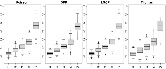
Figure 1: Boxplots of the difference in mean scores $\bar{s}_{j}-\bar{s}_{0}$ for $j=1,\ldots,5$ and the scoring function $S$ from Example 4. From left to right, $\Phi$ is a Poisson point process, a Gaussian determinantal point process, a log-Gaussian Cox process, and an inhomogeneous Thomas process. Means are based on $N=100$ realizations, boxplots on $M=500$ replicates.

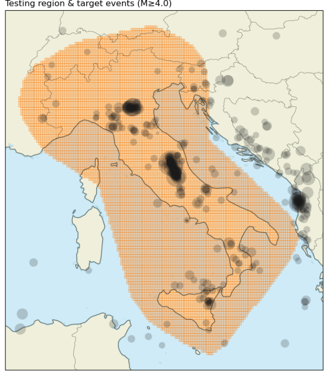
Figure 2: Testing region of the Italian CSEP experiment. Gray circles represent locations of M4+ earthquakes. Figure reproduced from Herrmann and Marzocchi, (2023).

5 Case study: Earthquake forecasting

In this case study we illustrate how consistent scoring functions can be used to compare earthquake forecasting models, and we shed new light on extant evaluation methods in seismology. All calculations are performed with R (R Core Team, , 2021).

5.1 Earthquake forecasting experiments

Over the past decades it has become consensus that earthquake forecasts ought to be probabilistic, i.e. instead of specifying whether or not an earthquake will occur, they provide a respective predictive distribution or aspects thereof (Jordan et al., , 2011). Satistical models to issue such forecasts are based on spatio-temporal point processes. They are usually specified via a conditional intensity (see (7)) that exhibits self-exciting behaviour, reflecting the conjecture that earthquakes trigger each other and cluster in space and time. An important example is the epidemic-type aftershock sequence (ETAS) model, see e.g. Kagan and Knopoff, (1987) and Ogata, (1988); Ogata (1998).

The Collaboratory for the Study of Earthquake Predictability (CSEP, see Introduction) evaluates earthquake forecasts prospectively in several regional testing centers with standardized testing routines. The prospective approach uses only forecasts submitted in real time before the respective outcomes are realized, which guarantees independence of the forecasts from actual observations. An important part of these routines is the earthquake likelihood model testing approach of Kagan and Jackson, (1995) and Schorlemmer et al., (2007), which we discuss in Section 5.3. Our case study relies on data from the operational earthquake forecasting system in Italy (OEF-Italy, Marzocchi et al., (2014)), which is based on the three independent short-term forecasting models that were tested prospectively in a CSEP testing center for the Italian testing region (Taroni et al., , 2018). See Figure 2 for an illustration.

The three independent models comprise LM (Lombardi and Marzocchi, , 2010) and FMC (Falcone et al., , 2010), which are ETAS-based models with distinct structure and calibration choices, and LG (Woessner et al., , 2010), which is based on the short-term earthquake probability (STEP) model of Gerstenberger et al., (2005) and composed of sub-models. We refer to the original references for more details about the individual models. OEF-Italy also includes an aggregated or ensemble forecast, namely, SMA, which predicts a weighted average of the above three models using the score model averaging (SMA) rule (Marzocchi et al., , 2012), with models being weighted inversely proportional to the log-likelihood of observed data. The SMA model is updated continuously based on new observations and was successfully applied to track the evolution of the recent earthquake sequence in central Italy in real time (Marzocchi et al., , 2017).

Our study considers earthquakes of magnitude greater or equal to four (M4+) between April 2005 and May 2020 (5520 days) that fall into the Italian CSEP testing region (Figure 2). The testing region is divided into 8993 grid cells. On each day, the four models produce forecasts for the expected number of M4+ earthquakes in the subsequent seven-day period for each grid cell. The forecasts are thus nonnegative values $x_{i,t}^{(j)}$ where $j$ denotes the model, $i$ the cell, and $t$ the day. They can then be compared to the observed number of events in each cell for that upcoming week. Since the forecasts concern seven-day periods, this number is only known seven days after a forecast was issued. For the same reason, the number of days available for evaluation reduces to 5514.

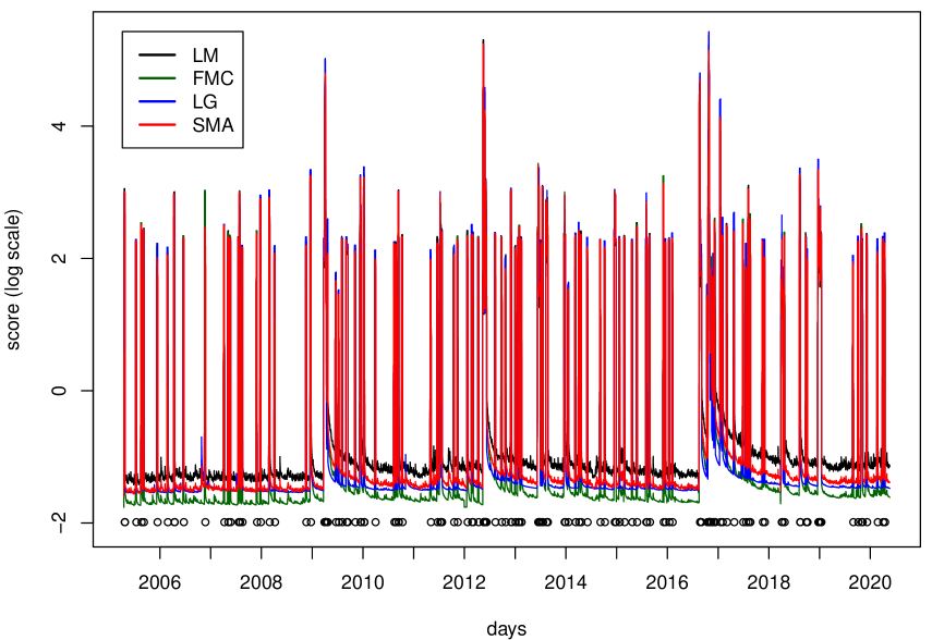
Figure 3: Daily scores $s_{j,t}$ from (10) based on $S_{\mathrm{pois}}$ for the four forecasting models from 2005 to 2020, logarithmic scale. The circles indicate the days of M4+ earthquakes and the tickmarks on the horizontal axis mark the first day of each year.

5.2 Model comparison and results

Since the models we consider produce mean forecasts, we have to employ (strictly) consistent scoring functions for the expectation functional for a sound comparison, see also Example 1. Such functions are of the Bregman form (2) and a natural choice is the quadratic score $S_{\mathrm{quad}}(x,y)=(x-y)^{2}$. However, the quadratic score focuses on no particular forecast cases in the sense of elementary scores (Ehm et al., , 2016). As an alternative that puts more emphasis on small forecast values and connects to the CSEP methods (see Section 5.3) we use the Poisson scoring function $S_{\mathrm{pois}}:(0,\infty)\times\mathbb{N}_{0}\to\mathbb{R}$ defined via

$$S_{\mathrm{pois}}(x,y)=-y\log(x)+x.$$ (9)

It is strictly consistent since it is a Bregman function corresponding to the strictly convex function $f(x)=x(\log(x)-1)$. Note that (9) can be interpreted as a discrete analogue to the Dawid-Sebastiani-score (Dawid and Sebastiani, , 1999), but with the normal distribution replaced by the Poisson distribution (Brehmer, , 2021). To obtain a daily score of the forecast models, the individual scores for the 8993 grid cells are summed up. The daily scores and the mean score of model $j$ are thus given by

$$s_{j,t}:=\sum_{i=1}^{8993}S\big{(}x_{i,t}^{(j)},\varphi_{t}(B_{i})\big{)}\qquad\text{ and }\qquad\bar{s}_{j}:=\frac{1}{5514}\sum_{t=1}^{5514}s_{j,t},$$ (10)

respectively, where $\varphi_{t}(B_{i})$ is the observed number of events in cell $B_{i}$ over the period from day $t$ to $t+6$. The mean score $\bar{s}_{j}$ estimates the expected score of model $j$ and is thus a measure of the relative forecast performance of this model. Figure 3 depicts the daily scores (10) based on $S_{\mathrm{pois}}$ for the four different models. It uses a logarithmic scale, because the values are much larger on days when events occur, in comparison to days without events. The FMC model consistently achieves the lowest scores on days without earthquakes, since it consistently forecasts the lowest number of events. However, overall the LM model shows the best performance in terms of mean scores over the whole testing period (10), as can be seen in Table 1. This conclusion applies under both the Poisson and the quadratic score.

Table 1: Summarized performance of the four models according to the mean score over the testing period $\bar{s}_{j}$ from (10). The scoring functions used for evaluation are the Poisson (“pois”) and the quadratic (“quad”) score. Lowest values in each column are in boldface.

Model	pois	quad
LM	2.68	0.8218
FMC	2.76	0.8269
LG	2.98	0.8275
SMA	2.70	0.8248

To understand why the overall scores indicate superior predictive ability of the LM model, we compute the mean score difference between model $j$ and model $j^{\prime}$ for each grid cell $i$ via

$$\Delta_{i}^{(j,j^{\prime})}:=\frac{1}{5514}\sum_{t=1}^{5514}\big{(}S_{\mathrm{pois}}(x_{i,t}^{(j)},\varphi_{t}(B_{i}))-S_{\mathrm{pois}}(x_{i,t}^{(j^{\prime})},\varphi_{t}(B_{i}))\big{)}.$$ (11)

The left part of Figure 4 plots $\Delta_{i}^{(1,2)}$, i.e. the mean score differences between the LM and the FMC model per grid cell. It illustrates that the lower mean score of the LM model stems from its good performance in central Italy in comparison to the FMC model. The right part illustrates aggregated performance, i.e. each pixel shows the performance when the forecasts and observed values within a square neighbourhood centred at this pixel are added up. In this case the neighbourhood has an edge length of 11 pixels. Again, better predictive ability of the LM model is most pronounced in central Italy and to a lesser extent in the north, i.e. in areas where earthquake sequences occurred during the study period. The opposite is true for marine regions around Sicily.

Figure 4: Mean score difference based on $S_{\mathrm{pois}}$ (11) between the LM and the FMC model, without (left) and with (right) aggregation. Negative values (blue) indicate that the LM model has superior forecast performance, and positive values (red) vice versa.

Often, lack of data complicates the forecasting of point processes as well as the proper testing of proposed forecasting models. This circumstance raises the question of how much data is needed to reach valid conclusions on superior predictive ability. As noted above, a commonly used tool is the Diebold–Mariano test (Diebold and Mariano, 1995), which is a one-sample $t$-test applied to the score differentials, with adaptations to time series settings. Standard power calculations for $t$-tests apply to independent samples, where rules of thumb for the calculation of a required sample size or a detectable difference are available (Lehr, , 1992; van Belle, , 2008). In time series settings, rules of this type also require adaptation, as exemplified in Section S4 of the Supplementary Material, which contains details on the analyses in this section.

5.3 A new perspective on earthquake likelihood model testing

An important element of the CSEP forecast experiments is a model evaluation approach introduced by Kagan and Jackson, (1995) and Schorlemmer et al., (2007), to which we refer as earthquake likelihood model testing (ELMT). Further conceptual and computational improvements are due to Zechar et al., 2010a , Rhoades et al., (2011), and Ogata et al., (2013).

Put simply, ELMT represents earthquakes by points in some region $\mathcal{X}\subset\mathbb{R}^{k}$, which is partitioned into grid cells $B_{1},\ldots,B_{N}$ for some $N\in\mathbb{N}$, see e.g. Figure 2. The data consist of values $x_{1},\ldots,x_{N}\in\mathbb{N}_{0}$ which count the earthquakes falling in each cell. A forecast or “model” is given by values $\lambda_{1},\ldots,\lambda_{N}\in(0,\infty)$ and its “log-likelihood” (Schorlemmer et al., , 2007) is defined as a sum of Poisson log-likelihoods, i.e. via

$$\ell(\lambda_{1},\ldots,\lambda_{N},x_{1},\ldots,x_{N})=\sum_{i=1}^{N}\left(x_{i}\log\lambda_{i}-\log(x_{i}!)-\lambda_{i}\right).$$ (12)

This terminology is motivated by the fact that, for a Poisson point process with intensity measure $\Lambda$ such that $\Lambda(B_{i})=\lambda_{i}$, for $i=1,\ldots,N$, (12) is the log-likelihood of the observation $x_{1},\ldots,x_{N}$. Based on (12), Schorlemmer et al., (2007) propose different tests. Here we only consider the test designed to compare forecasts.

The R-test, or ratio test, compares two forecasts $A$ and $B$ specified by their grid cell values $\lambda_{i}^{A}$ and $\lambda_{i}^{B}$ for $i=1,\ldots,N$, and aims to check whether model $A$ is at least as good as model $B$. The R-test considers the “log-likelihood ratio” based on (12), i.e.

$$R(A,B,x_{1},\ldots,x_{N})=\ell(\lambda_{1}^{A},\ldots,\lambda_{N}^{A},x_{1},\ldots,x_{N})-\ell(\lambda_{1}^{B},\ldots,\lambda_{N}^{B},x_{1},\ldots,x_{N}),$$ (13)

and then compares the realized value $z:=R(A,B,x_{1},\ldots,x_{N})$ to the distribution of the random variable $Z:=R(A,B,X_{1},\ldots,X_{N})$, where $X_{1},\ldots,X_{N}$ are independent Poisson random variables with parameters $\lambda_{i}^{A}$ for $i=1,\ldots,N$. If $z$ lies in the lower tail of the distribution of $Z$, then model $A$ is deemed worse than model $B$. As the distributional assumptions on $X_{1},\ldots,X_{N}$ demonstrate, there is an asymmetry inherent in the R-test: If model $A$ is tested against model $B$, then the $X_{i}$ are assumed to have parameters $\lambda_{i}^{A}$ and if $B$ is tested against $A$, then $\lambda_{i}^{B}$ are assumed for $X_{i}$. As noted by Rhoades et al., (2011) this implies that the R-test is not really a comparative test, but rather a goodness-of-fit test. This explains seemingly contradictory results observed in practice, where R-tests deem $A$ worse than $B$ and vice versa, see also Bray and Schoenberg, (2013) for a discussion. As a remedy, Rhoades et al., (2011) propose two modifications of the R-test, which do not rely on a Poisson assumption to determine the distribution of $Z$.

As pointed out by Harte, (2015), ELMT suffers from several drawbacks. First, relying on a partition leads to a loss of information, since the behaviour of models inside cells does not affect the evaluation. Moreover, assuming independence across cells as well as a Poisson distribution leads to a likelihood mis-specification under general point process models. This prohibits the testing of model characteristics other than cell expectations, since by reporting $(\lambda_{i})_{i=1,\ldots,N}$, every forecast is treated like a Poisson point process. However, as mentioned by Bray and Schoenberg, (2013), it is unclear how big the impact of the Poisson assumption is on the testing results.

Taking the perspective of consistent scoring functions, we can answer this question and clarify the role of the testing assumptions. To formalize ELMT in our setting, assume that the bounded domain $\mathcal{X}$ is partitioned into $k_{n}$ grid cells $\mathcal{T}_{n}=\{B_{1},\ldots,B_{k_{n}}\}$. Based on (12) and (13) we define the cell scoring function $S_{\mathrm{cell}}^{\mathcal{T}_{n}}:(0,\infty)^{k_{n}}\times\mathbb{M}_{0}\to\mathbb{R}$ via

$$S_{\mathrm{cell}}^{\mathcal{T}_{n}}(\lambda_{1},\ldots,\lambda_{k_{n}},\varphi)=\sum_{i=1}^{k_{n}}-\varphi(B_{i})\log(\lambda_{i})+\lambda_{i}$$ (14)

for each partition $\mathcal{T}_{n}$, $n\in\mathbb{N}$. If $k_{n}=N$ and $x_{i}=\varphi(B_{i})$ for $i=1,\ldots,N$, then (13) can be understood as the score difference between the forecasts $\lambda_{i}^{A}$ and $\lambda_{i}^{B}$ with respect to $S_{\mathrm{cell}}^{\mathcal{T}_{n}}$. Since it applies the scoring function (9) to each grid cell, $S_{\mathrm{cell}}^{\mathcal{T}_{n}}$ is strictly consistent for the collection of cell expectations $\mathbb{E}\Phi(B_{i})$, $B_{i}\in\mathcal{T}_{n}$, cf. Example 1. This shows that the Poisson log-likelihood in (13) can be used for a sound comparison of cell expectations, since the true expectations obtain the minimal expected score. We emphasize that this conclusion holds regardless of whether or not the data or the forecasts are based on Poisson point processes. Moreover, dependence among cells is irrelevant for this fact, since (strict) consistency concerns only expected scores. Hence, the validity of statistical methods which rely on the expected scores of (14) is not limited to Poisson models nor to Poisson point process data. In a nutshell, these methods assess forecast performance in terms of cell expectations only, since the scoring function (9) is strictly consistent for the expectation. For instance, the symmetric modifications of the R-test due to Rhoades et al., (2011) can be seen as Diebold–Mariano (DM) tests (Diebold and Mariano, 1995) based on $S_{\mathrm{cell}}^{\mathcal{T}_{n}}$. Hence, they test whether one model is better than its competitor in forecasting the mean number of earthquakes in the cells. Note that although such methods are valid for arbitrary point processes, considerable spatial or temporal dependencies will affect significance levels and deteriorate their ability to detect differences in forecast performance in finite samples.

It remains to discuss the role of the partitioning of $\mathcal{X}$ into grid cells. To understand its implications, note that just as the Poisson distribution leads to the scoring function (9) for the expectation, the Poisson point process can be used to obtain a scoring function for the intensity (Section 3.3). The reason is that every intensity report induces a Poisson point process with this intensity and these processes can then be compared via the logarithmic score (5), which attains the value (6) for Poisson densities. In the setting of Section 3.3, we can formalize as follows.

Proposition 3.

Let every element of $\mathcal{M}_{\rm f}$ admit a density $\lambda$ with respect to Lebesgue measure. Then the scoring function $S:\mathcal{M}_{\rm f}\times\mathbb{M}_{0}\to\mathbb{R}$ defined by

$$S(\Lambda,\{y_{1},\ldots,y_{n}\})=-\sum_{i=1}^{n}\log\lambda(y_{i})+\int_{\mathcal{X}}\lambda(y)\,\mathrm{d}y$$ (15)

for $n\in\mathbb{N}$, and $S(\Lambda,\emptyset)=\int_{\mathcal{X}}\lambda(y)\,\mathrm{d}y$, is a strictly consistent scoring function for the intensity.

Proof.

The scoring function (15) corresponds to $S$ from Proposition 2 when choosing the logarithmic score for $S^{\prime}$, the Bregman function (9) for $b$ and $c=1$. Since $S^{\prime}$ is strictly consistent and $b$ is strict, $S$ is strictly consistent for the intensity. ∎

The scoring function (15) can be interpreted as a point process analogon to the Dawid-Sebastiani-score (Dawid and Sebastiani, , 1999). While the Dawid-Sebastiani-score relies on the first and second moments of the predictive distribution, this scoring function depends on the intensity only.

The next result shows that the cell scoring function $S_{\mathrm{cell}}^{\mathcal{T}_{n}}$ serves as an approximation to the scoring function (15). Essentially, if a forecaster does not report an intensity $\lambda$, but only the integrals $\lambda_{i}^{(n)}$ of $\lambda$ over the collection of grid cells ${\mathcal{T}_{n}}$, then forecast comparison using the cell scoring function $S_{\mathrm{cell}}^{\mathcal{T}_{n}}$ is on par with a comparison based on the scoring function (15), provided the partition is sufficiently fine. The correction term in (16) does not affect the evaluation, as it is independent of the reported integrals. To make this precise, we follow Daley and Vere-Jones (2003) and call a sequence of partitions $(\mathcal{T}_{n})_{n\in\mathbb{N}}$ dissecting if it is nesting and asymptotically separates every pair of points.

Proposition 4.

Let $\lambda:\mathcal{X}\to(0,\infty)$ be an intensity and $(\mathcal{T}_{n})_{n\in\mathbb{N}}$ a dissecting system of measurable partitions of $\mathcal{X}$ which generates the Borel $\sigma$-algebra on $\mathcal{X}$. Let $P_{0}\in\mathcal{P}$ be the distribution of the unit rate Poisson point process on $\mathcal{X}$ and define partition integrals

$$\lambda_{i}^{(n)}=\int_{B_{i}^{(n)}}\lambda(y)\,\mathrm{d}y,$$

for all $i=1,\ldots,k_{n}$, $B_{i}^{(n)}\in\mathcal{T}_{n}$, and $n\in\mathbb{N}$. Then

$$S_{\mathrm{cell}}^{\mathcal{T}_{n}}\big{(}\lambda_{1}^{(n)},\ldots,\lambda_{k_{n}}^{(n)},\varphi\big{)}+\sum_{i=1}^{k_{n}}\mathbbm{1}(\varphi(B_{i}^{(n)})>0)\log(|B_{i}^{(n)}|)\longrightarrow S(\Lambda,\varphi),$$ (16)

for $P_{0}$-a.e. $\varphi\in\mathbb{M}_{0}$ as $n\to\infty$, where $S$ is the scoring function (15).

Proof.

Let $\varphi=\{y_{1},\ldots,y_{m}\}$ with $m\in\mathbb{N}_{0}$ be a point process realization. For a large $n\in\mathbb{N}$ every set $B_{i}^{(n)}$ contains at most one point of $\varphi$, and we let $i_{n}(j)$ denote the index of the set such that $y_{j}\in B_{i_{n}(j)}^{(n)}$ for $j=1,\ldots,m$. Then the left-hand side of (16) equals

$$\phantom{=}-\sum_{i=1}^{k_{n}}\left(\varphi(B_{i}^{(n)})\log\Big{(}\int_{B_{i}^{(n)}}\lambda(y)\,\mathrm{d}y\Big{)}-\mathbbm{1}(\varphi(B_{i}^{(n)})>0)\log(|B_{i}^{(n)}|)-\int_{B_{i}^{(n)}}\lambda(y)\,\mathrm{d}y\right)$$

$$=-\sum_{j=1}^{m}\log\left(|B_{i_{n}(j)}^{(n)}|^{-1}\int_{B_{i_{n}(j)}^{(n)}}\lambda(y)\,\mathrm{d}y\right)+\int_{\mathcal{X}}\lambda(y)\,\mathrm{d}y$$

$$\longrightarrow-\sum_{j=1}^{m}\log(\lambda(y_{j}))+\int_{\mathcal{X}}\lambda(y)\,\mathrm{d}y$$

for $n\to\infty$ and $P_{0}$-a.e. $\varphi\in\mathbb{M}_{0}$. The last line follows from an approximation result for the Radon-Nikodým derivative $\lambda$ (Daley and Vere-Jones, 2003, Lemma A1.6.III). ∎

Propositions 3 and 4 show that comparisons based on the Poisson log-likelihood (13) can be understood as approximations to a comparison of intensity forecasts with the scoring function (15). In particular, we can conclude that partitioning is not essential for model evaluation: A straightforward generalization of ELMT relies on models that produce intensities $\lambda:\mathcal{X}\to(0,\infty)$ on the testing region, which can then be compared via consistent scoring functions (Section 3.3), with (15) giving one possible choice. However, in some situations partitioning might be desirable, e.g. when no explicit expression for the intensity is available. This also applies to our case study, where only the expected numbers per grid cell were produced by the forecasting models. In light of Proposition 4, our evaluation is essentially a comparison of the point process intensities forecasted by the four competing models.

6 Discussion

Assessing forecast accuracy and comparing the performance of several competing forecasts is a non-trivial task that poses challenges across disciplines and sectors. In this paper we have demonstrated that consistent scoring functions allow for the comparative evaluation of point process forecasts. Our methods are complementary to the simulation-based approach of Heinrich-Mertsching et al. (2021), encompass existing techniques for model comparison, and yield a novel understanding of earthquake likelihood model testing. In particular, we have shown that the Poisson log-likelihood can be used for theoretically principled comparative forecast evaluation in terms of cell expectations. This is an important finding, as it supports current practice in comparisons between Poisson models, for which the interpretation in terms of log-likelihood is useful and welcome, and other types of models, which might generate cell expectations only. When one ignores the possibility of multiple events in a cell, the cell expectation equals the probability of an event, and we are in the setting studied by Serafini et al., (2022).

To conclude our study, we continue the discussion of methods for model comparison that are based on the log-likelihood, i.e. the model log-density evaluated at the observations, distinguish relative and absolute performance assessment, and hint at future work.

The entropy score considers the log-likelihood of probability forecasts induced by a point process model (Daley and Vere-Jones, , 2004; Harte and Vere-Jones, , 2005). It can be interpreted as an application of the logarithmic score to probabilistic predictions in terms of numbers of events. The expected value of the entropy score difference between a model of interest and a reference model yields the information gain. Daley and Vere-Jones, (2004) note that the information gain is an inherent characteristic of a point process model that quantifies predictability and relates closely to entropy. A detailed discussion of the relationships between proper scoring rules, entropy, and divergences is available in Section 2.2 of Gneiting and Raftery (2007).

Information criteria such as AIC or BIC assess the relative quality of competing models, and can be applied to point process models, provided that densities are available, see e.g. Chen et al., (2018). They connect naturally to consistent scoring functions through their goodness-of-fit component, which usually consists of a log-likelihood and thus finds the logarithmic score (3) for the model at hand. The penalty component, which depends on the number of fitted parameters, is a necessary correction when operating in-sample, i.e. relying on the same data as used for model fitting. In contrast, comparative forecast evaluation via scoring functions is tailored to out-of-sample settings, as in our case study.

In Bayesian settings, a standard approach to model comparison is the use of Bayes factors of a model vs. a competitor, as employed by Marzocchi et al., (2012) in earthquake likelihood model testing. Similar to information criteria, Bayes factors are closely connected to the logarithmic score (Gneiting and Raftery, 2007, Section 7).

A further likelihood-based method for point processes uses deviance residuals, as proposed by Clements et al., (2011). In general, point process residuals form an empirical process arising from fitting a conditional intensity to data (Schoenberg, , 2003; Baddeley et al., , 2005; Bray et al., , 2014). Residuals can be used to assess goodness-of-fit and especially indicate in which regions a model fits well or poorly. Clements et al., (2011) propose a graphic comparison of models for the conditional intensity by plotting the log-likelihood ratio across a partition of the spatial domain, which can be interpreted as visualizing local differences in the logarithmic score.

Consistent scoring functions, as well as the just discussed methods, compare competing models or forecasts. This contrasts with many existing point process model evaluation tools, which focus on absolute performance, e.g. based on calibration (Thorarinsdottir, , 2013) and goodness-of-fit. Although this is important in model building, a selection among the available competitors has to be done eventually, and measures of absolute performance are not designed, and hence tend to be poorly positioned, for this task. Moreover, as pointed out by Nolde and Ziegel (2017), focusing on absolute performance may lead to misguided incentives in designing candidate models.

Earthquake likelihood model testing, a central element of the CSEP forecasting experiments, is tacitly based on strictly consistent scoring functions for expectations. A principled use of these functions, as illustrated in our case study, provides valid comparisons of forecasted intensities. Importantly, common assumptions in the context of CSEP tests are not needed for such an evaluation: Neither the forecasting models, nor the data, need to follow any Poisson or independence assumption, and with suitably adapted models, partitioning the testing region can be avoided. As these conclusions apply to intensity forecasts, a natural next step is to employ consistent scoring functions to compare earthquake forecasts in terms of other statistical properties. In particular, dependence properties or full distributions are natural candidates for forecast evaluation in the CSEP framework (Schorlemmer et al., , 2018; Nandan et al., , 2019). The choice and implementation of consistent scoring functions in settings of this type pose challenges for future work.

Acknowledgements

Jonas Brehmer and Tilmann Gneiting are grateful for support by the Klaus Tschira Foundation. Jonas Brehmer gratefully acknowledges support by the German Research Foundation (DFG) through Research Training Group RTG 1953. Part of this research came to fruition during mutual visits of Kirstin Strokorb at the University of Mannheim and Jonas Brehmer and Martin Schlather at Cardiff University during a workshop funded by the London Mathematical Society. We thank our hosting institutions for their generous hospitality. The authors would also like to thank Claudio Heinrich-Mertsching, Christopher Dörr and Alexander Jordan for helpful discussions, and Kristof Kraus for code review. Likewise, we are grateful to the anonymous reviewers for their comments that helped improve the clarity of this paper.

Supplementary Material

The Supplementary Material contains additional technical details and further simulation experiments. R code for reproduction is publicly available (Brehmer, , 2023). Data are available from the authors upon request.

indtceContents

Supplement to:
Comparative evaluation of point process forecasts

S1 Discussion of point process scenarios

This section extends the discussion at the end of Section 2.

In the main manuscript we focus on the setting where a spatial point process $\Phi$ on some domain $\mathcal{X}\subset\mathbb{R}^{d}$ is observed at fixed points in time. For example, the case study (Section 5) considers daily observations of locations of earthquakes in Italy. However, forecasting for point processes appears in a variety of other situations, and the use of strictly consistent scoring functions adapts readily. To clarify this idea, we distinguish three different point process scenarios. Although motivated by commonly encountered applications, there might be settings where the distinction is artificial.

Scenario A (purely spatial) In this scenario, the process is defined on either a single spatial domain (Scenario A1), or several non-overlapping subdomains (Scenario A2). Examples include points fixated by observers of images (Barthelmé et al., 2013) and locations of trees in a forest (Stoyan and Penttinen, 2000). Stationarity is a common simplifying assumption in this context.

Scenario B (purely temporal) In this scenario, there is no spatial component and the process concerns points in time only. Examples are arrival times of e-mails (Fox et al., 2016) and times of infection with a disease (Schoenberg et al., 2019). In this special setting the directional character of time allows for a distinct interpretation and treatment.

Scenario C (spatio-temporal) In addition to the spatial component, processes in this scenario possess a temporal component, which could be discrete (Scenario C1) or continuous (Scenario C2). Examples include locations and times of crimes in a city (Mohler et al., 2011) and earthquakes observed over time in a specific region (Ogata, 1998; Zhuang et al., 2002). The main manuscript focuses on Scenario C1.

In order to compare forecasts in each of these scenarios, we can in principle proceed as in Sections 4 and 5: Choose a strictly consistent scoring function $S$ for a statistical property of point processes, e.g. the intensity, and find the mean score difference

$$\frac{1}{n}\sum_{i=1}^{n}\left(S(r_{i},\varphi_{i})-S(r_{i}^{*},\varphi_{i})\right)$$

for forecast reports $r_{i}$ and $r_{i}^{*}$ and associated observed point patterns $\varphi_{i}$, where the index $i=1,\ldots,n$ represents repeated observations. Then negative values support forecast $r$, while positive values support $r^{*}$. The mean score difference is an estimator of the expected score difference $\mathbb{E}\left(S(r,\Phi)-S(r^{*},\Phi)\right)$, and implementation details vary across scenarios, also impacting the assessment of the uncertainty inherent in the estimate, which is of particular importance when tests for superior predictive performance are sought. To illustrate the key ideas we distinguish whether the point process has a continuous or discrete time component.

Discrete time

Assume that the point process is sampled at fixed points in time, i.e. it can be modelled by a sequence $(\Phi_{t})_{t\in\mathbb{N}}$ adapted to a filtration $(\mathcal{H}_{t})_{t\in\mathbb{N}}$. This setting includes the special case of i.i.d. realizations and relates to Scenario C1 as well as variants of Scenario A with repeated observations. Given two forecast sequences $(R_{t})_{t\in\mathbb{N}}$ and $(R_{t}^{*})_{t\in\mathbb{N}}$ the score differences $(S(R_{t},\Phi_{t})-S(R_{t}^{*},\Phi_{t}))_{t\in\mathbb{N}}$ form a sequence of real-valued random variables, thus the common Diebold–Mariano (DM) tests (Diebold and Mariano, 1995) are directly applicable. We briefly discuss the more general forecast comparison framework of Nolde and Ziegel (2017) in our setting. Let $S$ be strictly consistent for a point process statistic $\Gamma:\mathcal{P}\to\mathsf{A}$ and assume that forecasts in terms of $\Gamma$ applied to the conditional distribution $\Phi_{t}\mid\mathcal{H}_{t-1}$ are given. These forecasts can be regarded as random sequences $R=(R_{t})_{t\in\mathbb{N}}$ and $R^{*}=(R_{t}^{*})_{t\in\mathbb{N}}$ such that $R_{t}$ and $R^{*}_{t}$ are $\mathcal{H}_{t-1}$-measurable. Their forecast performance can be compared via the mean score difference

$$\Delta_{n}(R,R^{*}):=\frac{1}{n}\sum_{t=1}^{n}S(R_{t},\Phi_{t})-\frac{1}{n}\sum_{t=1}^{n}S(R_{t}^{*},\Phi_{t})=\frac{1}{n}\sum_{t=1}^{n}\left(S(R_{t},\Phi_{t})-S(R_{t}^{*},\Phi_{t})\right),$$ (S1)

which is an estimator for the difference in expected scores. Based on the law of large numbers and the strict consistency of $S$, a positive value supports the hypothesis that $R^{*}$ is superior to $R$, while a negative value supports the opposite hypothesis. A further step is to test whether $\Delta_{n}(R,R^{*})$ is significantly different from zero. In the simple situation of an i.i.d. sequence $(\Phi_{t})_{t\in\mathbb{N}}$, the forecast sequences reduce to $r,r^{*}\in\mathsf{A}$, i.e. they are constant in time. We can then test for significant differences in expected scores based on the asymptotic normality of the well-known $t$-statistic $t_{n}:=\sqrt{n}\Delta_{n}(r,r^{*})/\sqrt{\hat{\sigma}_{n}^{2}}$, where $\hat{\sigma}_{n}^{2}$ estimates the variance of $S(r,\Phi)-S(r^{*},\Phi)$. For dependent time series $(\Phi_{t})_{t\in\mathbb{N}}$, $(R_{t})_{t\in\mathbb{N}}$, and $(R_{t}^{*})_{t\in\mathbb{N}}$ we refer to Nolde and Ziegel (2017), where tests for equal forecast performance rely on suitable asymptotic results developed in Giacomini and White (2006).

Continuous time

If we consider point processes in Scenario C2 or Scenario B, then temporal dependence between the points of $\Phi$ becomes an essential feature of the process and can also be object of the forecast. For instance, the statistic $\Gamma$ might consist of temporal features of the point process. Also, dependencies need to be accounted for in estimation and testing, as they affect asymptotic distributions. To illustrate this, assume for simplicity that $\Phi$ is a purely temporal process observed over a time period $[0,T]$ with $0<t_{1}<\cdots<t_{k}<T$ denoting the corresponding arrival times. Moreover, let $R_{i}$ and $R_{i}^{*}$ be reports issued at time $t_{i-1}$ based on the previous arrivals $t_{1},\ldots,t_{i-1}$. This yields a realized score difference

$$\Delta_{T}(R,R^{*}) =\sum_{i=1}^{n(T)}\left(S(R_{i},t_{i})-S(R_{i}^{*},t_{i})\right),$$ (S2)

where $n(T):=\Phi((0,T])$ is the random number of points in $[0,T]$. In contrast to (S1) we do not consider averages since $n(T)$ is a random variable depending on $\Phi$ and dividing by it will interfere with the consistency of $S$. The score difference $\Delta_{T}(R,R^{*})$ is a sum of a random number of random variables, usually called a random sum. This perspective connects the estimation of score differences to the theory of total claim amount in insurance, see e.g. Mikosch (2009) and Embrechts et al. (1997).

Asymptotic results for the score difference (S2) for $T\to\infty$ are desirable to assess how uncertainty affects forecast evaluation and transfer the DM test to the continuous time setting. One possible approach to this problem relies on limit theorems for randomly indexed processes due to Anscombe (1952), in particular random central limit theorems: If the number of points $n(T)$ satisfies a weak law of large numbers, then under Anscombe’s condition, we only need to ensure that the sequence $(S(R_{i},t_{i})-S(R_{i}^{*},t_{i}))_{i\in\mathbb{N}}$ satisfies a central limit theorem in order to obtain asymptotic normality for (S2). Such results are available for strong mixing (Lee, 1997), $\psi$-weakly dependent (Hwang and Shin, 2012), and $m$-dependent (Shang, 2012) sequences. Working these into tests for superior forecast performance for (spatio-)temporal point processes is an avenue for future work.

S2 Further scoring functions for point processes

The technical context of this section is the same as in Section 3.

S2.1 Simple examples

The subsequent examples are applications of the transformation principle (Proposition 1).

Example S1 (void probability).

For any fixed set $B\in\mathcal{B}(\mathcal{X})$ the functional $\Gamma$ defined via $\Gamma(P)=P(\{\varphi\mid\varphi\cap B=\emptyset\})$ is elicitable. This follows from Proposition 1 with $T(F)=\mathbb{E}_{F}Y$ and $g(\varphi)=\mathbbm{1}(\varphi(B)=0)$. Strictly consistent scoring functions for $\Gamma$ are of the Bregman form (2), see also Example 1.

Example S2 (point process integrals).

Fix measurable functions $f_{i}:\mathcal{X}\to\mathbb{R}$, $i=1,\ldots,m$ for $m\in\mathbb{N}$. Define $g:\mathbb{M}_{0}\to\mathbb{R}^{m}$ via

$$g(\varphi)=\left(\int_{\mathcal{X}}f_{1}\,\mathrm{d}\varphi,\ldots,\int_{\mathcal{X}}f_{m}\,\mathrm{d}\varphi\right)^{\top}=\left(\sum_{x_{i}\in\varphi}f_{1}(x_{i}),\ldots,\sum_{x_{i}\in\varphi}f_{m}(x_{i})\right)^{\top},$$

set $g(\mathcal{P}):=\{P\circ g^{-1}\mid P\in\mathcal{P}\}$ and let $T=\mathrm{id}_{g(\mathcal{P})}$. Then the finite-dimensional distribution functional $\Gamma_{f_{1},\ldots,f_{m}}(P)=T(P\circ g^{-1})$ is an elicitable property of the point process $\Phi$. Consistent scoring functions for $\Gamma$ are obtained by applying consistent scoring functions for distributions (Gneiting and Raftery, 2007) to the $m$-variate distribution $P\circ g^{-1}$, see also Heinrich-Mertsching et al. (2021).

S2.2 Distribution and density

This material extends Section 3.2.

General result for the full distribution

The law $P_{\Phi}$ of a finite point process on $\mathcal{X}$ can be equivalently represented by two sequences $(p_{k})_{k\in\mathbb{N}_{0}}$ and $(\Pi_{k})_{k\in\mathbb{N}}$. Each $p_{k}$ specifies the probability of finding $k$ points in a realization. The $\Pi_{k}$ are symmetric probability measures on $\mathcal{X}^{k}$ which describe the distribution of any ordering of points, given $k$ points are realized, see Daley and Vere-Jones (2003, Chapter 5.3) for details.

To state the next result, we introduce the notion of symmetric scoring functions, where $S:\mathsf{A}\times\mathbb{R}^{n}\to\mathbb{R}$ is called symmetric if $S(a,y_{1},\ldots,y_{n})=S(a,y_{\pi(1)},\ldots,y_{\pi(n)})$ for all $a\in\mathsf{A}$, $y\in\mathbb{R}^{n}$ and permutations $\pi$. Symmetry ensures that the scoring functions in the subsequent proposition are independent of the enumeration of the realization of $\Phi$.

Proposition S1.

Let $\mathcal{P}$ be a class of distributions of finite point processes, with $Q\in\mathcal{P}$ decomposed into $(\Pi_{k}^{Q})_{k\in\mathbb{N}}$ and $(p_{k}^{Q})_{k\in\mathbb{N}_{0}}$. Set $\mathcal{F}_{k}:=\{\Pi_{k}^{Q}\mid Q\in\mathcal{P}\}$ and let $S_{k}:\mathcal{F}_{k}\times\mathcal{X}^{k}\rightarrow\mathbb{R}$ be a symmetric consistent scoring function for $\mathrm{id}_{\mathcal{F}_{k}}$ for all $k\in\mathbb{N}$. Let $S_{0}$ be a consistent scoring function for distributions on $\mathbb{N}_{0}$. Then the function $S:\mathcal{P}\times\mathbb{M}_{0}\to\mathbb{R}$ defined via

$$S(((\Pi_{k}^{Q})_{k\in\mathbb{N}},(p_{k}^{Q})_{k\in\mathbb{N}_{0}}),\{y_{1},\ldots,y_{n}\})=S_{n}(\Pi_{n}^{Q},y_{1},\ldots,y_{n})+S_{0}((p_{k}^{Q})_{k\in\mathbb{N}_{0}},n)$$

for $n\in\mathbb{N}$ and $S(((\Pi_{k}^{Q})_{k\in\mathbb{N}},(p_{k}^{Q})_{k\in\mathbb{N}_{0}}),\emptyset):=S_{0}((p_{k}^{Q})_{k\in\mathbb{N}_{0}},0)$ is a consistent scoring function for the distribution of the point process $\Phi$. It is strictly consistent if $S_{0}$ and $(S_{k})_{k\in\mathbb{N}}$ are strictly consistent.

Proof.

The result follows by decomposing the expectation $\mathbb{E}_{P}S(Q,\Phi)$ into expectations on the sets $\{\Phi=n\}$ for $n\in\mathbb{N}$ and using the (strict) consistency of $S_{n}$ on each set. ∎

Hyvärinen score

Assume that a point process model admits explicit expressions for the Janossy densities $(j_{k})_{k\in\mathbb{N}_{0}}$ (see Section 3.2), however, only up to an unknown normalizing constant. In this situation, 0-homogeneous consistent scoring functions for densities can be of use, as they allow for the consistent evaluation of an unnormalized density. The most relevant example is the Hyvärinen score defined via

$$\mathrm{HyvS}(f,y):=\Delta\log f(y)+\frac{1}{2}\|\nabla\log f(y)\|^{2},$$

where $\nabla$ denotes the gradient, $\Delta$ is the Laplace operator, and $f$ is a twice differentiable density on $\mathbb{R}^{d}$. To ensure strict consistency on a class of probability densities $\mathcal{L}$ its members have to be positive almost everywhere and for all $f,g\in\mathcal{L}$ it must hold that $\nabla\log(f(y))g(y)\to 0$ as $\|y\|\to\infty$, see Hyvärinen (2005), Parry et al. (2012), and Ehm and Gneiting (2012) for details.

Similar to the logarithmic score, we can transfer the Hyvärinen score to the point process setting. To do this we assume that for all $Q\in\mathcal{P}$ and $k\in\mathbb{N}$, $j_{k}^{Q}$ is defined on $(\mathbb{R}^{d})^{k}$ and satisfies the aforementioned regularity conditions. Then the function $S:\mathcal{P}\times\mathbb{M}_{0}\to\mathbb{R}$ defined via

$$S((j_{k}^{Q})_{k\in\mathbb{N}_{0}},\{y_{1},\ldots,y_{n}\})=\mathrm{HyvS}(j_{n}^{Q},y_{1},\ldots,y_{n})$$ (S3)

for $n\in\mathbb{N}$ and $S((j_{k}^{Q})_{k\in\mathbb{N}_{0}},\emptyset):=0$ is a consistent scoring function for the distribution of the point process $\Phi$. Observe that we cannot achieve strict consistency for $S$, since the probability of $|\Phi|=n$ is proportional to $j_{n}$ and thus not accessible to the Hyvärinen score.

Example S3 (Gibbs point process).

Stemming from theoretical physics, Gibbs processes are a popular tool to model particle interactions. They are defined via their Janossy densities

$$j_{n}(y_{1},\ldots,y_{n})=C(\theta)\exp\left(-\theta U(y_{1},\ldots,y_{n})\right),$$

where $U$ represents point interactions, $\theta$ is a parameter often referred to as temperature, and $C$ is the partition function, which ensures that the collection $(j_{k})_{k\in\mathbb{N}_{0}}$ is properly normalized, see e.g. Daley and Vere-Jones (2003, Chapter 5.3) and Chiu et al. (2013, Chapter 5.5). It is in general difficult to find closed form expressions for $C$, or even to approximate it, hence the Hyvärinen score might seem attractive to evaluate models based on $(j_{k})_{k\in\mathbb{N}_{0}}$. Plugging $j_{n}$ into (S3) gives

$$S((j_{k})_{k\in\mathbb{N}_{0}},\{y_{1},\ldots,y_{n}\})=\theta\left(-\Delta U(y_{1},\ldots,y_{n})+\frac{\theta}{2}\|\nabla U(y_{1},\ldots,y_{n})\|^{2}\right)$$

for $n\in\mathbb{N}$, where the derivatives are computed with respect to the coordinates of the vector $(y_{1},\ldots,y_{n})\in(\mathbb{R}^{d})^{n}$. The simplest choice for interactions is to restrict $U$ to first- and second-order terms

$$U(y_{1},\ldots,y_{n}):=\sum_{i=1}^{n}l(y_{i})+\sum_{i,j=1}^{n}\psi\left(\|y_{i}-y_{j}\|^{2}\right)$$

for $l:\mathbb{R}^{d}\to\mathbb{R}$ and $\psi:[0,\infty)\to[0,\infty)$ with $\psi(0)=0$, see e.g. Daley and Vere-Jones (2003, Chapter 5.3). To apply the Hyvärinen score in this setting, $l$ and $\psi$ have to satisfy regularity conditions detailed above and in Hyvärinen (2005), and in particular admit second order derivatives almost everywhere. The soft-core models for $\psi$ introduced in Ogata and Tanemura (1984) satisfy this condition, while their hard-core model for $\psi$ is not even continuous. An additional technical issue is that Ogata and Tanemura (1984) consider point processes on a finite domain $\mathcal{X}$ and use a constant $l$. To make the Hyvärinen score applicable in this setting a possible solution is to approximate their models via twice differentiable densities on $(\mathbb{R}^{d})^{n}$.

S2.3 Moment measures

Moment measures can be interpreted as the point process analogue to the moments of a univariate random variable. Strictly consistent scoring functions for these measures can be constructed in the same way as for the intensity, see Proposition 3.4.

For $n\in\mathbb{N}$, let $\mathcal{M}_{\rm f}^{n}=\mathcal{M}_{\rm f}(\mathcal{X}^{n})$ be the set of finite Borel measures on $\mathcal{X}^{n}$. For positive measurable functions $f:\mathcal{X}^{n}\to(0,\infty)$ the $n$-th moment measure $\mu^{(n)}$ and the $n$-th factorial moment measure $\alpha^{(n)}$ are defined via the relations

$$\mathbb{E}\left(\underset{x_{1},\ldots,x_{n}\in\Phi}{\sum}f(x_{1},\ldots,x_{n})\right) =\int_{\mathcal{X}^{n}}f(x_{1},\ldots,x_{n})\,\mathrm{d}\mu^{(n)}(x_{1},\ldots,x_{n}),$$

and

$$\mathbb{E}\left(\underset{x_{1},\ldots,x_{n}\in\Phi}{\sum\nolimits^{\neq}}f(x_{1},\ldots,x_{n})\right) =\int_{\mathcal{X}^{n}}f(x_{1},\ldots,x_{n})\,\mathrm{d}\alpha^{(n)}(x_{1},\ldots,x_{n}),$$

respectively, see e.g. Chiu et al. (2013) and Daley and Vere-Jones (2003). Here $\Sigma^{\neq}$ denotes summation over all $n$-tuples that contain distinct points of $\Phi$. Using the notion of factorial product defined via

$$m^{[n]}:=\left\{\begin{array}[]{lr}m(m-1)(m-2)\cdots(m-n+1)&,\,m\geq n\\ 0&,\,m<n\end{array}\right.$$

for $m,n\in\mathbb{N}$ we obtain the concise representations $\mu^{(n)}(B^{n})=\mathbb{E}\Phi(B)^{n}$ and $\alpha^{(n)}(B^{n})=\mathbb{E}\Phi(B)^{[n]}$ for Borel sets $B\in\mathcal{B}(\mathcal{X})$, see e.g. Daley and Vere-Jones (2003, Chapter 5).

Proposition S2.

Set $\mathcal{F}^{n}:=\{P^{*}\mid P\in\mathcal{M}_{\rm f}^{n}\}$, let $S:\mathcal{F}^{n}\times\mathcal{X}^{n}\rightarrow\mathbb{R}$ be a consistent scoring function for $\mathrm{id}_{\mathcal{F}^{n}}$ and $b:[0,\infty)\times[0,\infty)\rightarrow\mathbb{R}$ a Bregman function.

1. The function $S_{1}:\mathcal{M}_{\rm f}^{n}\times\mathbb{M}_{0}\to\mathbb{R}$ defined via

   $$S_{1}(\mu,\{y_{1},\ldots,y_{m}\})=\underset{x_{1},\ldots,x_{n}\in\{y_{1},\ldots,y_{m}\}}{\sum}S(\mu^{*},x_{1},\ldots,x_{n})+c\hskip 0.7113ptb(\mu(\mathcal{X}^{n}),m^{n})$$

   for $m\in\mathbb{N}$, and $S_{1}(\mu,\emptyset)=c\hskip 0.7113ptb(\mu(\mathcal{X}^{n}),0)$ for $c>0$, is a consistent scoring function for the $n$-th moment measure.

2. The function $S_{2}:\mathcal{M}_{\rm f}^{n}\times\mathbb{M}_{0}\to\mathbb{R}$ defined via

   $$S_{2}(\alpha,\{y_{1},\ldots,y_{m}\})=\underset{x_{1},\ldots,x_{n}\in\{y_{1},\ldots,y_{m}\}}{\sum\nolimits^{\neq}}S(\alpha^{*},x_{1},\ldots,x_{n})+c\hskip 0.7113ptb(\alpha(\mathcal{X}^{n}),m^{[n]})$$

   for $m\geq n$ and $S_{2}(\alpha,\{y_{1},\ldots,y_{m}\})=c\hskip 0.7113ptb(\alpha(\mathcal{X}^{n}),0)$ for $m<n$ and with $c>0$ is a consistent scoring function for the $n$-th factorial moment measure.

Both $S_{1}$ and $S_{2}$ are strictly consistent if $S$ is strictly consistent and $b$ is strict.

In many cases of interest $\alpha^{(n)}$ is absolutely continuous with respect to Lebesgue measure on $\mathcal{X}^{n}$ and its density $\varrho^{(n)}$ is called product density, see e.g. Chiu et al. (2013). A (strictly) consistent scoring function for $\varrho^{(n)}$ can be obtained from Proposition S2 (ii) by choosing $S$ to be a (strictly) consistent scoring function for densities.

Example S4.

Let $n=2$ and for simplicity consider the product density $\varrho^{(2)}$ of a stationary and isotropic point process. In this situation, $\varrho^{(2)}$ depends on the point distances only, i.e. it can be represented via $\varrho^{(2)}(x_{1},x_{2})=\varrho^{(2)}_{0}(\|x_{1}-x_{2}\|)$ for some $\varrho^{(2)}_{0}:[0,\infty)\to[0,\infty)$. Analogous to Example 4, we can use the quadratic score for $b$ and the logarithmic score for $S$ in Proposition S2 (ii). This gives the strictly consistent scoring function

$$S(\varrho^{(2)},\{y_{1},\ldots,y_{m}\}) =-\underset{x_{1},x_{2}\in\{y_{1},\ldots,y_{m}\}}{\sum\nolimits^{\neq}}\log(\varrho^{(2)}_{0}(\|x_{1}-x_{2}\|))$$

$$\phantom{=}+m^{[2]}\log|\varrho^{(2)}|+c\,(|\varrho^{(2)}|-m^{[2]})^{2},$$

where $c>0$ is some scaling constant. Simulation experiments in Section S3.2 show how $S$ compares different product density forecasts.

S2.4 Summary statistics

Summary statistics of point processes are central tools to quantify point interactions such as clustering or inhibition. This subsection constructs strictly consistent scoring functions for the frequently used $K$-function. Throughout we assume that $\Phi$ is a stationary point process on $\mathbb{R}^{d}$, i.e. any translation of the process by $x\in\mathbb{R}^{d}$, which we denote via $\Phi_{x}$, has the same distribution as $\Phi$. This implies that the intensity measure of $\Phi$ is a multiple of Lebesgue measure and can be represented via some $\lambda>0$, see e.g. Chiu et al. (2013, Chapter 4.1).

A common way to describe a stationary point process is to consider its properties in the neighbourhood of $x\in\mathbb{R}^{d}$, given that $x$ is a point in $\Phi$. Due to stationarity, the location of $x$ is irrelevant and thus it is usually referred to as the “typical point” of $\Phi$. The technical tool to describe the behaviour around this point is the Palm distribution of $\Phi$, denoted via $\mathbb{P}_{0}$ for probabilities and $\mathbb{E}_{0}$ for expectations. It satisfies the defining identity

$$\lambda\,|W|\,\mathbb{E}_{0}f(\Phi)=\mathbb{E}\left(\sum_{x\in\Phi\cap W}f(\Phi_{-x})\right)$$

for all measurable functions $f:\mathbb{M}_{0}\to\mathbb{R}$ such that the expectations are finite, and it is independent of the observation window $W\in\mathcal{B}(\mathbb{R}^{d})$ (Illian et al., 2008, Chapter 4). When we need to highlight the distribution of the point process, we write $\mathbb{E}_{P,0}$ for the Palm expectation given $\Phi$ has distribution $P\in\mathcal{P}$.

Denote the $d$-dimensional ball of radius $r>0$ around zero via $B_{r}=B(0,r)$. The K-function of $\Phi$ is defined via

$$K:(0,\infty)\to[0,\infty),\quad r\mapsto\frac{\mathbb{E}_{0}\Phi\left(B_{r}\backslash\{0\}\right)}{\lambda},$$

and it quantifies the mean number of points in a ball around the “typical point” of $\Phi$, see e.g. Chiu et al. (2013) and Illian et al. (2008) for details. Deriving strictly consistent scoring functions for the K-function appears challenging since it combines the Palm distribution and the intensity. However, in many situations both of these quantities are of interest. We thus derive a result which defines scoring functions for joint reports of the $K$-function and the intensity. Our point process property of interest is thus $\Gamma(P):=(\lambda_{P},K_{P})$, where the subscript denotes the dependence of the quantities on the distribution $P\in\mathcal{P}$ of the process $\Phi$. Since observation windows are always finite, we fix some $r^{*}>0$ and let $K_{P}$ be the restriction of the $K$-function to the interval $(0,r^{*})$.

To derive consistent scoring functions let us fix some $r\in(0,r^{*})$ and assume for now that $\lambda_{P}$ is known and that instead of data we directly observe the Palm distribution of $\Phi$. In this simplified situation, $K_{P}(r)$ is just an expectation with respect to $\mathbb{P}_{0}$, hence “consistent scoring functions” for it are of the Bregman form

$$S(x,\varphi)=-f(\lambda_{P}x)-f^{\prime}(\lambda_{P}x)\big{(}\varphi(B_{r}\backslash\{0\})-\lambda_{P}x\big{)},$$ (S4)

for a convex function $f:(0,\infty)\to\mathbb{R}$, see Theorem 1 and Example 1. This is because $\mathbb{E}_{P,0}b(x,\Phi)\geq\mathbb{E}_{P,0}b(K_{P}(r),\Phi)$ holds for all $x\geq 0$ and $P\in\mathcal{P}$. To arrive at a strictly consistent scoring function for the functional $\Gamma$ three steps remain: Firstly, we have to include a consistent scoring function for the first component of $\Gamma$, i.e. the intensity. Moreover, we need to integrate (S4) with respect to $r$ in order to evaluate the $K$-function on the entire interval $(0,r^{*})$. Finally, we have to account for the fact that we can not observe $\mathbb{P}_{0}$, but only points of $\Phi$ on some closed and bounded observation window $W\subset\mathbb{R}^{d}$. Hence, we need to compute the expected score $\mathbb{E}_{0}S(x,\Phi)$ via an expectation of $\Phi$ on $W$. Such problems lead to edge corrections, i.e. additional terms to account for the fact that (unobserved) points outside of $W$ affect the estimation near the boundary of $W$, see e.g. Chiu et al. (2013, Chapter 4.7) for details. Since (S4) is linear in $\varphi$, edge corrections for the expected score are equivalent to edge corrections for the expectation $\mathbb{E}_{0}\Phi(B_{r}\backslash\{0\})$, which are well-known in the context of $K$-function estimation. Before we formalize these three steps in a proposition, we state a result needed for the proof, see Gneiting (2011, Theorem 4).

Lemma S1 (revelation principle).

Let $\mathsf{A},\mathsf{A}^{\prime}$ be some sets and $g:\mathsf{A}\rightarrow\mathsf{A}^{\prime}$ a bijection with inverse $g^{-1}$. Let $T:\mathcal{F}\rightarrow\mathsf{A}$ and $T_{g}:\mathcal{F}\rightarrow\mathsf{A}^{\prime}$ defined via $T_{g}(F):=g(T(F))$ be functionals. Then $T$ is elicitable if and only if $T_{g}$ is elicitable. A function $S:\mathsf{A}\times\mathsf{O}\rightarrow\mathbb{R}$ is a (strictly) consistent scoring function for $T$ if and only if $S_{g}:\mathsf{A}^{\prime}\times\mathsf{O}\rightarrow\mathbb{R}$, $(x,y)\mapsto S_{g}(x,y):=S(g^{-1}(x),y)$ is a (strictly) consistent scoring function for $T_{g}$.

Proposition S3.

Let $b_{1},b_{2}:[0,\infty)\times[0,\infty)\rightarrow\mathbb{R}$ be Bregman functions and $w:(0,\infty)\to[0,\infty)$ a weight function. Define $\mathcal{C}:=\{K_{P}\mid P\in\mathcal{P}\}$, a set of possible $K$-functions, and let $\kappa$ satisfy $\mathbb{E}_{P}\kappa(B_{r},\Phi\cap W)=\lambda_{P}\mathbb{E}_{P,0}\Phi(B_{r}\backslash\{0\})$ for all $P\in\mathcal{P}$ and $r\in(0,r^{*})$. Then the function $S:((0,\infty)\times\mathcal{C})\times\mathbb{M}_{0}\to\mathbb{R}$ defined via

$$S((\lambda,K),\varphi)=b_{1}(\lambda,\varphi(W)|W|^{-1})+\int_{0}^{r^{*}}b_{2}(\lambda^{2}K(r),\kappa(B_{r},\varphi))w(r)\,\mathrm{d}r$$

is consistent for the point process property $\Gamma(P):=(\lambda_{P},K_{P})$, where the second component is restricted to $(0,r^{*})$. It is strictly consistent if $b_{1}$ and $b_{2}$ are strict and $w$ is strictly positive.

Proof.

Using Theorem 1, the Fubini-Tonelli theorem, and

$$\mathbb{E}_{P}\kappa(B_{r},\Phi)=\lambda_{P}\mathbb{E}_{P,0}\Phi(B_{r}\backslash\{0\})=\lambda_{P}^{2}K_{P}(r)$$

for $r\in(0,r^{*})$, standard arguments show that the scoring function

$$S^{\prime}((\lambda,h),\varphi):=b_{1}(\lambda,\varphi(W)|W|^{-1})+\int_{0}^{r^{*}}b_{2}(h(r),\kappa(B_{r},\varphi))w(r)\,\mathrm{d}r,$$

where $h:(0,\infty)\to(0,\infty)$ is an increasing function, is consistent for the property $\Gamma^{\prime}(P):=(\lambda_{P},\lambda_{P}^{2}K_{P}(r))$. An application of the revelation principle (Lemma S1) gives (strict) consistency for $\Gamma$. ∎

Similar to Proposition 2, this result blends two scoring components, namely the expected number of points and their distances. Hence, choosing suitable Bregman functions $b_{1}$ and $b_{2}$ in applications, again leads to issues of balancing the magnitudes of different scoring components. A similarly intricate question is the choice of $\kappa$. Relevant choices result from the construction of estimators for the $K$-function, which are often based on dividing $\kappa$ by an estimator for $\lambda^{2}$. A common choice is

$$\kappa_{\mathrm{st}}(B_{r},\varphi):=\underset{x_{1},x_{2}\in\varphi\cap W}{\sum\nolimits^{\neq}}\frac{\mathbbm{1}_{B_{r}}(x_{2}-x_{1})}{|W_{x_{1}}\cap W_{x_{2}}|},$$

where $W_{z}:=\{x+z\mid x\in W\}$ is the shifted observation window and $r$ is such that $|W\cap W_{z}|$ is positive for all $z\in B_{r}$, see e.g. Illian et al. (2008, Chapter 4.3) and Chiu et al. (2013, Chapter 4.7). An alternative arises via minus-sampling, i.e. by reducing the observation window $W$ in order to reduce edge effects. This yields

$$\kappa_{\mathrm{minus}}(B_{r},\varphi):=\frac{1}{|W|}\underset{x_{1},x_{2}\in\varphi\cap W,\,x_{2}\in W\ominus r}{\sum\nolimits^{\neq}}\mathbbm{1}_{B_{r}}(x_{2}-x_{1}),$$

where $W\ominus r:=\{x\mid B(x,r)\subset W\}$ is the reduced observation window and $r<\operatorname{diam}(W)/2$. For other choices of $\kappa$, most notably for isotropic point processes, see Chiu et al. (2013, Chapter 4.7).

Practitioners usually rely on the $L$-function, a modification of the $K$-function, which is defined via $L(r)=\sqrt[d]{K(r)/\beta_{d}}$ for $r\geq 0$, where $\beta_{d}:=|B_{1}|$. It satisfies $L(r)=r$ for the Poisson point process, and thus normalizes the $K$-function such that it is independent of the dimension $d$ for a Poisson point process (Chiu et al., 2013). A (strictly) consistent scoring function for the $L$-function follows immediately from Proposition S3 and another application of the revelation principle. The explicit formula follows by replacing the first component of $b_{2}$ by $\lambda^{2}L(r)^{d}\beta_{d}$ in Proposition S3. The idea underlying the construction of scoring functions for the $K$- and $L$-function presented here can be transferred to other summary statistics for stationary point processes.

S3 Extended simulation study

S3.1 Intensity

This subsection extends Section 4. We give more details on the used point processes and provide a closer analysis of the simulation experiments in the main paper. We then perform additional simulations with a different scoring function and study the approximation derived in Proposition 4.

All experiments rely on the six intensities defined in Section 4, see Figure S5 for an illustration. We consider two strictly consistent scoring functions for the intensity. The first choice is used in Section 4 and given by

$$S_{1}(\Lambda,\{y_{1},\ldots,y_{n}\})=-\sum_{i=1}^{n}\log(\lambda(y_{i}))+n\log|\Lambda|+c\,(|\Lambda|-n)^{2},$$ (S5)

see also Example 3.5. Our second choice is

$$S_{2}(\Lambda,\{y_{1},\ldots,y_{n}\})=-\sum_{i=1}^{n}\log\lambda(y_{i})+\int_{\mathcal{X}}\lambda(y)\,\mathrm{d}y,$$ (S6)

which is defined in Proposition 5.1 and appears as the limit scoring function in earthquake likelihood model testing, see Section 5.3. The scaling factor $c>0$ in (S5) is set to $c=1/10$. We draw $N=100$ i.i.d. samples and repeat $M=500$ times.

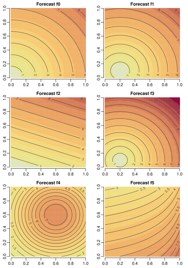
Figure S5: Heat maps of the intensity forecasts $f_{0},\ldots,f_{5}$, see Section 4.

Details on the point process models

We consider four different data-generating processes for $\Phi$ on $[0,1]^{2}$, all of which have (approximate) intensity $f_{0}(x,y)=6\sqrt{x^{2}+y^{2}}$. The models are specified as follows:

1. An inhomogeneous Poisson point process with intensity $f_{0}$.

2. A thinned Gaussian determinantal point process (DPP), see e.g. Hough et al. (2006) and Lavancier et al. (2015). In general, a DPP is a locally finite point process with product densities (see Section S2.3) given by

   $$\varrho^{(n)}(x_{1},\ldots,x_{n})=\det\left(C(x_{i},x_{j})\right)_{i,j=1,\ldots,n}$$

   for $n\in\mathbb{N}$, where $C:\mathbb{R}^{d}\times\mathbb{R}^{d}\to\mathbb{R}$ is a covariance. As a result, the DPP’s intensity function is $x\mapsto C(x,x)$ and it is stationary and isotropic whenever its covariance is. We choose $C(x_{1},x_{2})=C_{0}(\|x_{1}-x_{2}\|)$, where $C_{0}:[0,\infty)\to\mathbb{R}$ is the Gaussian covariance function

   $$C_{0}(r)=\sigma^{2}\exp\left\{-\left(\frac{r}{s}\right)^{2}\right\},$$ (S7)

   with variance $\sigma^{2}=\max_{x,y\in[0,1]}f_{0}(x,y)$ and scale $s=6/100$. We then apply independent thinning to the homogeneous Gaussian DPP in order to obtain the final point process with intensity function $f_{0}$.

3. An inhomogeneous log-Gaussian Cox process (LGCP), see e.g. Illian et al. (2008, Chapter 6). A LGCP is a Poisson point process conditional on a random intensity function arising from a log-Gaussian random field. If $\mu:\mathbb{R}^{d}\to\mathbb{R}$ is the mean and $C:\mathbb{R}^{d}\times\mathbb{R}^{d}\to\mathbb{R}$ is the covariance of the random field, then the LGCP has intensity function

   $$x\mapsto\exp\left(\mu(x)+\frac{1}{2}C(x,x)\right).$$

   We choose $C(x_{1},x_{2})=C_{0}(\|x_{1}-x_{2}\|)$, where $C_{0}:[0,\infty)\to\mathbb{R}$ is the exponential covariance function

   $$C_{0}(r)=\sigma^{2}\exp\left(-\frac{r}{s}\right),$$ (S8)

   with variance $\sigma^{2}=1/4$ and scale $s=1/5$. The mean is set to $\mu(x)=\log(f_{0}(x))-1/8$ such that the intensity equals $f_{0}$.

4. An inhomogeneous Thomas cluster process, see e.g. Illian et al. (2008, Chapter 6). This is a cluster process which arises from an inhomogeneous Poisson point process as parent and a random number of cluster points which are drawn from a normal distribution centred at its parent point. As intensity of the parent process we choose $2f_{0}/3$ and the number of points per cluster follows a Poisson distribution with parameter $3/2$. The location of each cluster point is determined by a normal distribution which is centred at the parent point and where the components are uncorrelated and have standard deviation $0.05$. As a result of the clustering, the intensity of the Thomas process is only approximately equal to $f_{0}$.

Table S1: Fraction of replicates where the “row forecast” was preferred over the “column forecast” by a standard DM test with level $\alpha=0.05$ based on the scoring function $S_{1}$ (S5) and $M=500$ replicates

Poisson $f_{0}$ $f_{1}$ $f_{2}$ $f_{3}$ $f_{4}$ $f_{5}$ $f_{0}$ 0.45 0.81 0.96 0.99 1.00 $f_{1}$ 0.00 0.40 0.88 0.82 0.99 $f_{2}$ 0.00 0.00 0.28 0.69 0.98 $f_{3}$ 0.00 0.00 0.01 0.24 0.91 $f_{4}$ 0.00 0.00 0.00 0.01 0.97 $f_{5}$ 0.00 0.00 0.00 0.00 0.00

DPP $f_{0}$ $f_{1}$ $f_{2}$ $f_{3}$ $f_{4}$ $f_{5}$ $f_{0}$ 0.52 0.83 0.97 0.99 1.00 $f_{1}$ 0.00 0.39 0.91 0.80 1.00 $f_{2}$ 0.00 0.00 0.27 0.67 0.97 $f_{3}$ 0.00 0.00 0.01 0.22 0.93 $f_{4}$ 0.00 0.00 0.00 0.01 0.98 $f_{5}$ 0.00 0.00 0.00 0.00 0.00

LGCP $f_{0}$ $f_{1}$ $f_{2}$ $f_{3}$ $f_{4}$ $f_{5}$ $f_{0}$ 0.48 0.80 0.93 0.99 1.00 $f_{1}$ 0.00 0.39 0.85 0.81 1.00 $f_{2}$ 0.00 0.00 0.27 0.66 0.97 $f_{3}$ 0.00 0.00 0.01 0.19 0.92 $f_{4}$ 0.00 0.00 0.00 0.01 0.97 $f_{5}$ 0.00 0.00 0.00 0.00 0.00

Thomas $f_{0}$ $f_{1}$ $f_{2}$ $f_{3}$ $f_{4}$ $f_{5}$ $f_{0}$ 0.24 0.52 0.76 0.89 1.00 $f_{1}$ 0.00 0.26 0.60 0.56 0.91 $f_{2}$ 0.00 0.00 0.18 0.44 0.81 $f_{3}$ 0.00 0.00 0.01 0.14 0.68 $f_{4}$ 0.00 0.00 0.00 0.01 0.78 $f_{5}$ 0.00 0.00 0.00 0.00 0.00

Further details for the experiments of Section 4

Section 4 presents four simulation experiments based on the scoring function $S_{1}$. Table S1 shows the results of DM tests (see Diebold and Mariano (1995) and Section S1) for these experiments. For each of the $M=500$ realizations we test whether forecast $f_{i}$ (row) achieves the same expected score as forecast $f_{j}$ (column). The rejection frequencies in favour of $f_{0}$ against $f_{j}$, $j=1,\ldots,5$ (first row of each table) are generally in line with the mean score differences in Figure 1. Moreover, the results of the DM tests are similar for all four simulation experiments. In the third and fourth experiment (lower part of Table S1) the frequencies of rejection in favour of the optimal forecast $f_{0}$ (first row of each table) decrease slightly for the LGCP and substantially for the Thomas process. An intuitive reason for this is that clustering, which is a feature of both processes, complicates the distinction between different intensity forecasts.

Experiments with a different scoring function

We now investigate how the forecast comparison changes when using the scoring function $S_{2}$ instead of the scoring function $S_{1}$ from Section 4. Boxplots of mean score differences are given in Figure S6 and they are generally similar to the ones presented in Figure 1.

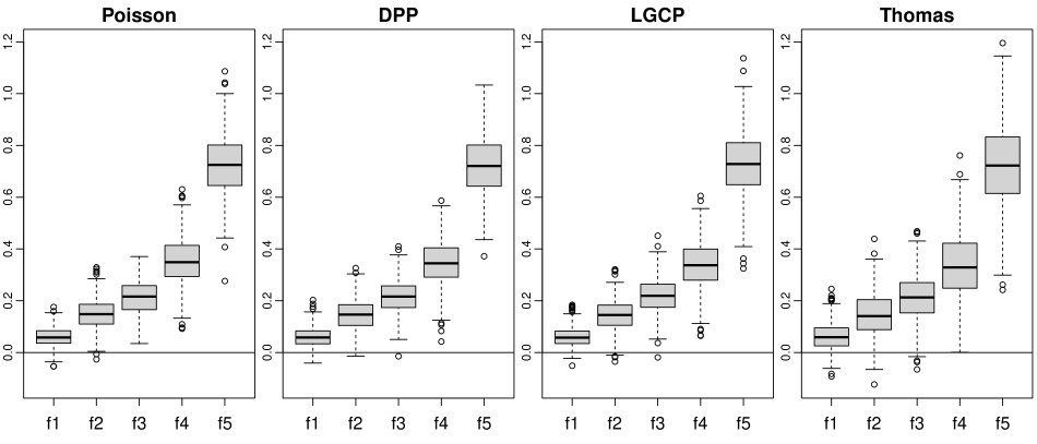
Figure S6: Boxplot of difference in mean scores $\bar{s}_{j}-\bar{s}_{0}$ for $j=1,\ldots,5$ and scoring function $S_{2}$ (S6). From left to right, $\Phi$ is a Poisson point process, a Gaussian determinantal point process, a log-Gaussian Cox process, or an inhomogeneous Thomas process. Means are based on $N=100$ realizations, boxplots on $M=500$ replicates.

The same conclusion holds for the results of DM tests given in Table S2 resemble those in Table S1. This suggests that in our experiments the choice of $c=1/10$ for $S_{1}$ leads to a similar balance of shape and total mass of the intensity as with $S_{2}$. However, in other forecast settings, or with a different choice of $c$, the two scoring functions may lead to differing conclusions. As in the previous experiments, the clustering of the LGCP and the Thomas process leads to less conclusive decisions between the forecasts. In contrast, the inhibition of the Gaussian DPP seems to facilitate the comparison between the forecasts.

A further sequence of experiments considers the speed of convergence in Proposition 4, i.e. how well score differences based on $S_{\mathrm{cell}}^{\mathcal{T}_{n}}$, as defined in (14), approximate score differences based on $S_{2}$ (S6). We select a family of partitions $(\mathcal{T}_{n})_{n\in\mathbb{N}}$ of $[0,1]^{2}$ which arises from dyadic partitions of both axes. Specifically, each grid cell $B_{ij}^{(n)}\in\mathcal{T}_{n}$ is given by $[(i-1)/2^{n},i/2^{n}]\times[(j-1)/2^{n},j/2^{n}]$ for $i,j\in\{1,\ldots,2^{n}\}$. The number of cells is thus $k_{n}=2^{2n}$ and we choose $n\in\{1,\ldots,6\}$ for the simulations. As forecasts we rely on the intensity functions $f_{0},\ldots,f_{5}$ introduced in Section 4 which we transform into grid-based reports $f_{l,ij}^{(n)}$ by integrating $f_{l}$ over the grid cell $B_{ij}^{(n)}$. These reports are then compared to the number of points per cells via $S_{\mathrm{cell}}^{\mathcal{T}_{n}}$. We study the convergence of the rejection probabilities of DM tests based on $S_{\mathrm{cell}}^{\mathcal{T}_{n}}$ for $N=100$ i.i.d. samples of $\Phi$ and increasing $n$. The corresponding fractions converge to the values in Table S2, as illustrated in Figure S7 for the comparisons of $f_{0}$ to $f_{1},\ldots,f_{5}$. These simulations suggest that for forecasts which are far from the underlying truth $n=2$, i.e. 16 grid cells, is already enough to obtain DM results based on $S_{\mathrm{cell}}^{\mathcal{T}_{n}}$ which are in good agreement with the results based on $S_{2}$ (Table S2). For intensity functions closer to the truth, such as $f_{1}$, $n=3$, i.e. 64 grid cells, seems necessary to obtain a good approximation.

Table S2: Fraction of replicates where the “row forecast” was preferred over the “column forecast” by a standard DM test with level $\alpha=0.05$ based on the scoring function $S_{2}$ (S6) and $M=500$ replicates

Poisson

	$f_{0}$	$f_{1}$	$f_{2}$	$f_{3}$	$f_{4}$	$f_{5}$
$f_{0}$		0.46	0.84	0.95	0.99	1.00
$f_{1}$	0.00		0.48	0.87	0.84	1.00
$f_{2}$	0.00	0.00		0.24	0.70	0.98
$f_{3}$	0.00	0.00	0.01		0.29	0.94
$f_{4}$	0.00	0.00	0.00	0.00		0.96
$f_{5}$	0.00	0.00	0.00	0.00	0.00

DPP $f_{0}$ $f_{1}$ $f_{2}$ $f_{3}$ $f_{4}$ $f_{5}$ $f_{0}$ 0.47 0.84 0.96 0.99 1.00 $f_{1}$ 0.00 0.43 0.93 0.86 1.00 $f_{2}$ 0.00 0.00 0.22 0.69 0.98 $f_{3}$ 0.00 0.00 0.01 0.28 0.93 $f_{4}$ 0.00 0.00 0.00 0.01 0.97 $f_{5}$ 0.00 0.00 0.00 0.00 0.00

LGCP $f_{0}$ $f_{1}$ $f_{2}$ $f_{3}$ $f_{4}$ $f_{5}$ $f_{0}$ 0.44 0.79 0.93 0.98 1.00 $f_{1}$ 0.00 0.39 0.84 0.83 0.99 $f_{2}$ 0.00 0.00 0.27 0.68 0.96 $f_{3}$ 0.00 0.00 0.00 0.23 0.92 $f_{4}$ 0.00 0.00 0.00 0.01 0.97 $f_{5}$ 0.00 0.00 0.00 0.00 0.00

Thomas $f_{0}$ $f_{1}$ $f_{2}$ $f_{3}$ $f_{4}$ $f_{5}$ $f_{0}$ 0.24 0.53 0.73 0.86 0.99 $f_{1}$ 0.00 0.26 0.58 0.53 0.92 $f_{2}$ 0.00 0.01 0.16 0.42 0.80 $f_{3}$ 0.00 0.00 0.01 0.15 0.69 $f_{4}$ 0.00 0.00 0.00 0.01 0.79 $f_{5}$ 0.00 0.00 0.00 0.00 0.00

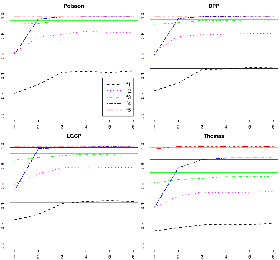
Figure S7: Fraction of replicates where $f_{0}$ was preferred over $f_{1},\ldots,f_{5}$ by a standard DM test with level $\alpha=0.05$ based on the scoring function $S_{\mathrm{cell}}^{\mathcal{T}_{n}}$, with $n$ varying along the horizontal axis, sample size $N=100$, and $M=500$ replicates. The solid lines represent the fractions resulting from the use of $S_{2}$ (see (S6)), as given in Table S2. The legend in the upper left plot applies to all other plots, too.

S3.2 Product density

This subsection presents simulation experiments for the product density (Section S2.3). We simulate stationary and isotropic point processes with three different second order structures corresponding to inhibition, clustering, and no interaction. We draw $N=30$ i.i.d. samples $\varphi_{i}$ from $\Phi$ and compare the mean scores for different forecasts, in the same way as in Section 4. The scoring function $S$ is defined in Example S4 and the scaling factor $c=10^{-5}$ is chosen such that the log and squared terms are of the same order of magnitude. We repeat the simulations $M=500$ times to assess the variation in mean scores.

Details on the point process models

We simulate three different stationary and isotropic data-generating processes $\Phi$ on the window $[0,1]^{2}$ with intensity $\lambda=25$. The models are specified as follows:

1. A LGCP which is determined by a stationary and isotropic Gaussian process with mean $\mu\in\mathbb{R}$ and covariance function $C_{0}$, see e.g. Illian et al. (2008). Its second order product density $\varrho^{(2)}:\mathbb{R}^{d}\times\mathbb{R}^{d}\to\mathbb{R}$ is given by $\varrho^{(2)}(x_{1},x_{2})=\varrho^{(2)}_{0}(\|x_{1}-x_{2}\|)$, where

   $$\varrho^{(2)}_{0}(r)=\exp\left(2\mu+C_{0}(0)+C_{0}(r)\right).$$

   We choose $C_{0}$ as the Gaussian covariance function (S7) with variance $\sigma^{2}=\log 2$ and scale $s=5/100$ and set $\mu=\log(\lambda)-\sigma^{2}/2$.

2. A homogeneous Poisson point process.

3. A DPP defined via the Gaussian covariance function (S7), see e.g. Hough et al. (2006) and Lavancier et al. (2015). Its second order product density is given by $\varrho^{(2)}(x_{1},x_{2})=\varrho^{(2)}_{0}(\|x_{1}-x_{2}\|)$, where

   $$\varrho^{(2)}_{0}(r)=C_{0}(0)^{2}-C_{0}(r)^{2},$$

   and $C_{0}$ is the Gaussian covariance (S7) with variance $\sigma^{2}=\lambda^{2}$ and scale $s=0.06$.

Forecast comparison

The three simulation experiments compare five different product density forecasts, which are based on stationary and isotropic point processes, see Example S4. Hence, the forecasts take the form $\varrho^{(2)}(x_{1},x_{2})=\varrho^{(2)}_{0}(\|x_{1}-x_{2}\|)$, with the function $\varrho^{(2)}_{0}$ given by

$$f_{1}(r) =\exp\left[2\mu+\sigma^{2}\left\{1+\exp(-400r^{2})\right\}\right]$$

$$f_{2}(r) =\exp\left[2\mu+\sigma^{2}\left\{1+\exp(-20r)\right\}\right]$$

$$f_{3}(r) =\lambda^{2}$$

$$f_{4}(r) =\lambda^{2}\left\{1-\exp(-2r/s)\right\}$$

$$f_{5}(r) =\lambda^{2}\left\{1-\exp(-2(r/s)^{2})\right\},$$

where $\mu=\log(\lambda)-\sigma^{2}/2$, $\sigma^{2}=\log(2)$, $s=0.06$, and $\lambda=25$. See Figure S8 for a graphical comparison of the different functions. The forecasts $f_{1}$ and $f_{2}$ represent clustering, since they arise as product densities of LGCPs with Gaussian or exponential covariance function (see (S7) and (S8)). The constant function $f_{3}$ corresponds to a homogeneous Poisson process. The forecasts $f_{4}$ and $f_{5}$ arise as product densities of DPPs with Gaussian or exponential covariance function and thus represent inhibition. Our parameter choices ensure that the point process models corresponding to $f_{1},\ldots,f_{5}$ all have intensity equal to $\lambda$, so forecast misspecifications only occur in the product density.

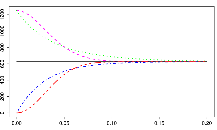
Figure S8: Plot of the five different choices for $\varrho^{(2)}_{0}:[0,\infty)\to[0,\infty)$ on which the product density forecasts in Section S3.2 are based. The first two ($f_{1}$ and $f_{2}$) represent clustering, the last two ($f_{4}$ and $f_{5}$) inhibition. The constant $f_{3}$ implies no interaction.

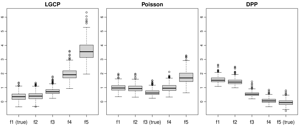
Figure S9: Boxplots of mean scores $\bar{s}_{j}$ for different product density forecasts, where $\Phi$ is a log-Gaussian Cox process (left), a homogeneous Poisson process (centre), or a Gaussian determinantal point process (right). Means are based on $N=30$ realizations, boxplots on $M=500$ replicates.

In the first experiment the true $\Phi$ is a LGCP with a Gaussian covariance function such that its product density corresponds to $f_{1}$. In the second experiment $\Phi$ is a homogeneous Poisson process with intensity $\lambda$, such that $f_{3}$ becomes the optimal forecast in this situation. Lastly, we let $\Phi$ be a DPP with Gaussian covariance function and parameters such that $f_{5}$ is optimal. We thus perform one experiment for each of the three phenomena clustering, no interaction, and inhibition.

The simulated mean scores are displayed in Figure S9 for all three experiments. The optimal forecast consistently achieves the lowest mean score. In the case of clustering (left subfigure) the LGCP related forecasts $f_{1}$ and $f_{2}$ perform roughly similar, while the misspecified no interaction and inhibition forecasts $f_{3}$, $f_{4}$ and $f_{5}$ lead to considerably higher mean scores. A similar, but mirrored behaviour is apparent in the inhibition experiment (right subfigure): The forecast $f_{4}$, which gets the nature of point interactions right, attains low mean scores, even though it is not optimal. The mean scores of the Poisson forecast $f_{3}$ are always in between the “extremes”. The DM test probabilities of the three experiments are given in Table S3 and support these observations. Additionally, the DM results illustrate that the clustering forecasts $f_{1}$ and $f_{2}$ are preferred more often over the inhibition forecast $f_{5}$ in the case of Poisson data (centre table).

Table S3: Fraction of times the “row forecast” was preferred over the “column forecast” by a standard DM test with level $\alpha=0.05$ in the product density experiments (Section S3.2), based on $M=500$ repetitions

LGCP

	$f_{1}$	$f_{2}$	$f_{3}$	$f_{4}$	$f_{5}$
$f_{1}$		0.18	0.63	0.99	1.00
$f_{2}$	0.00		0.57	0.99	1.00
$f_{3}$	0.00	0.00		1.00	1.00
$f_{4}$	0.00	0.00	0.00		1.00
$f_{5}$	0.00	0.00	0.00	0.00

DPP

	$f_{1}$	$f_{2}$	$f_{3}$	$f_{4}$	$f_{5}$
$f_{1}$		0.00	0.00	0.00	0.00
$f_{2}$	0.90		0.00	0.00	0.00
$f_{3}$	1.00	1.00		0.00	0.00
$f_{4}$	1.00	1.00	1.00		0.00
$f_{5}$	1.00	1.00	0.96	0.57

Poisson
$f_{1}$ $f_{2}$ $f_{3}$ $f_{4}$ $f_{5}$ $f_{1}$ 0.01 0.00 0.04 0.43 $f_{2}$ 0.17 0.00 0.06 0.50 $f_{3}$ 0.77 0.68 0.64 0.96 $f_{4}$ 0.07 0.05 0.00 1.00 $f_{5}$ 0.00 0.00 0.00 0.00

S4 Additional details for the case study

This material extends Section 5.2. Figure S10 reproduces Figure 3 but with the quadratic score $S_{\mathrm{quad}}$ rather than the Poisson score $S_{\mathrm{pois}}$. In contrast to Figure 3 we see that there are periods without events where the LG model rather than the FMC model attains the lowest scores.

Figures S12 and S12 use the same methods as in Figure 4 to compare the LM model to the LG and the SMA model. The regions of superior or inferior forecast performance of the LM model remain generally the same across the three comparisons. The right plots of these figures compare the forecasts after spatial aggregation, for which we give details now.

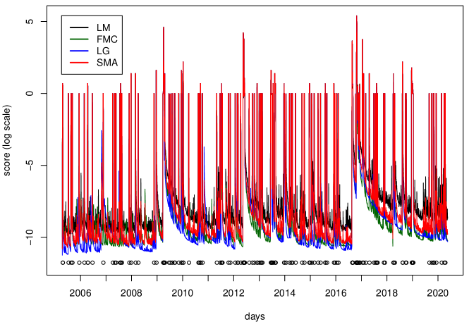
Figure S10: Daily scores $s_{j,t}$ from (10) based on $S_{\mathrm{quad}}$ for the four forecasting models from 2005 to 2020, logarithmic scale. The circles indicate the days of M4+ earthquakes and the tickmarks on the horizontal axis mark the first day of each year.

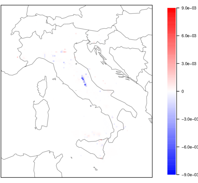
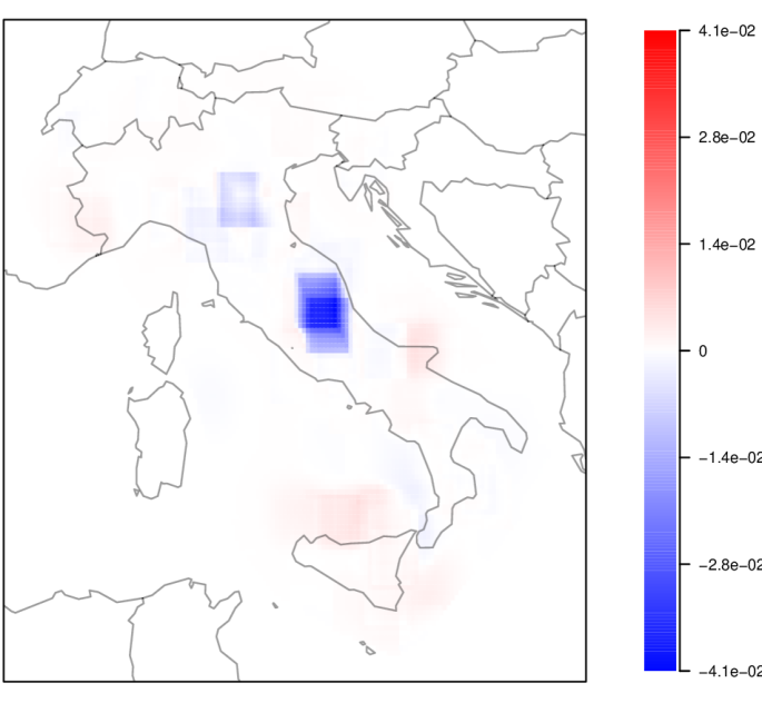
Figure S11: Mean score difference based on $S_{\mathrm{pois}}$ (11) between the LM and the LG model, without (left) and with (right) aggregation. Negative values (blue) indicate that the LM model has superior forecast performance, and positive values (red) vice versa.

Figure S12: Mean score difference based on $S_{\mathrm{pois}}$ (11) between the LM and the SMA model, without (left) and with (right) aggregation. Negative values (blue) indicate that the LM model has superior forecast performance, and positive values (red) vice versa.

S4.1 Spatial aggregation

We follow the notation of Section 5.2, except that we introduce a coordinate notation for the testing region (Figure 2). For each grid cell $B_{i}$ we now write $B_{k,l}$ where $k$ is the horizontal and $l$ the vertical coordinate. A cell with a higher value of $k$ is further east and a cell with a higher value of $l$ is further north. Similarly, let $x_{k,l,t}^{(j)}$ be the forecast of model $j$ corresponding to cell $B_{k,l}$ on day $t$. For combinations of $k$ and $l$ that fall outside the testing region we use the convention $x_{k,l,t}^{(j)}=0$ and $B_{k,l}=\emptyset$.

Let $\delta\in\mathbb{N}_{0}$ be a given level of aggregation. We define the locally aggregated forecast and the locally aggregated grid cell at coordinate $(k,l)$ and aggregation level $\delta$ via

$$\bar{x}_{k,l,t}^{(j)}:=\sum_{\mu=-\delta}^{\delta}\sum_{\nu=-\delta}^{\delta}x_{k+\mu,l+\nu,t}^{(j)}\qquad\text{ and }\qquad\bar{B}_{k,l}:=\bigcup_{\mu=-\delta}^{\delta}\bigcup_{\nu=-\delta}^{\delta}B_{k+\mu,l+\nu}$$

respectively. In the interior of the testing region, this is an aggregation of the forecasts over a square neighbourhood with edge length $2\delta+1$ centred at $(k,l)$. At the boundary of the testing region the aggregation neighbourhoods will be smaller, however, as there are almost no events in this area, this does not affect the plots. Due to the linearity of expectations, the values $\bar{x}_{k,l,t}^{(j)}$ are again valid mean forecasts that can be compared via consistent scoring functions, e.g. the Poisson score (9). The right plots of Figures 4, S12, and S12 show this comparison via the mean score difference of the locally aggregated forecasts

$$\bar{\Delta}_{k,l}^{(j,j^{\prime})}:=\frac{1}{5514}\sum_{t=1}^{5514}\big{(}S_{\mathrm{pois}}(\bar{x}_{k,l,t}^{(j)},\varphi_{t}(\bar{B}_{k,l}))-S_{\mathrm{pois}}(\bar{x}_{k,l,t}^{(j^{\prime})},\varphi_{t}(\bar{B}_{k,l}))\big{)},$$

where $\delta=5$. For $\delta=0$ there is no aggregation, so $\bar{\Delta}_{k,l}^{(j,j^{\prime})}$ simplifies to $\Delta_{i}^{(j,j^{\prime})}$, the (non-aggregated) mean score difference (11). For $\delta$ large enough there is essentially only one big grid cell and one forecasted number remaining. The corresponding plot would show only one colour, indicating the forecast performance of the models with respect to the total number of events in the testing region.

S4.2 Sample size considerations

Point process forecasting is often challenged by a lack of data, and particularly a lack of data to properly test newly proposed prediction models. In this light, a critical question is how much data is required to reach valid conclusions on superior predictive ability. As discussed, a commonly used tool is the Diebold–Mariano (DM) test, which is a one-sample $t$-test applied to the score differentials, with adaptations to time series settings. Standard power calculations for $t$-tests apply to independent samples, and a well known, crude rule of thumb (Lehr, , 1992; van Belle, , 2008) states that for a one-sample, two-tailed $t$-test with level 0.05, a sample size $n=8s^{2}/d^{2}$ yields an approximate power of 0.80, where $s^{2}$ is the variance of the score differentials, and $d$ is the difference to be detected. Phrased differently, if the variance $s^{2}$ and the sample size $n$ are given, a difference $d_{n}=(8s^{2}/n)^{1/2}$ is detectable, subject to the above specifications of the size and the power of the $t$-test.

In Tables S4 and S5 we return to Table 1 in the main paper, where we compare the predictive performance of the LM, FMC, LG, and SMA models, respectively. We show the mean score differential and its variance, and find the detectable difference $d_{5514}$ at the given sample size of $n=5514$ daily forecasts of earthquake activity over the subsequent seven-day period, for the Poisson score and the quadratic score, respectively. Figures S13 and S14 show the sample autocorrelation function for the score differentials. Not surprisingly, there is considerable dependency at lags up to about seven to nine days ahead, due to the overlap in the seven-day outlook, though autocorrelations are small to negligible at higher lags. As standard power calculations assume independent samples, a more appropriate quantification of a detectable difference is based on a sample size of $[5514/7]=787$. A further alternative is to use an estimate of the effective sample size (Thiébaux and Zwiers, 1984), which reduces the regular sample size according to the autocorrelation of the series, in line with the handling of dependencies in DM tests.

Interestingly, under both the Poisson and the quadratic score, and for each of the six binary model comparisons, the actual mean score differential $m$ tends to be nested in between the (overly) optimistic estimate $d_{5514}$ and the (arguably) realistic estimate $d_{787}$ for a detectable difference, which indicates that the comparative evaluation might reasonably be considered to be based on sufficient data. Evidently, this current analysis is crude and preliminary, using default specifications from the biostatistical literature for size and power, and we encourage follow-up studies.

Table S4: Mean $m$ and variance $s^{2}$ of the score differential, and detectable difference $d_{n}$ for sample size $n=787$ and $n=5514$ according to the rule of thumb by Lehr, (1992), under the Poisson score and for the models from Table 1 in the main paper.

Poisson score	LG$-$LM	LG$-$SMA	LG$-$FMC	FMC$-$LM	FMC$-$SMA	SMA$-$LM
Mean $m$	0.307	0.285	0.221	0.086	0.064	0.022
Variance $s^{2}$	11.936	6.438	4.885	2.542	0.695	0.983
$d_{5514}$	0.132	0.097	0.084	0.061	0.032	0.038
$d_{787}$	0.348	0.256	0.223	0.161	0.084	0.100

Table S5: Same as Table S4, but under the quadratic score. All entries are to be divided by a factor of 100.

Quadratic score	LG$-$LM	FMC$-$LM	SMA$-$LM	LG$-$SMA	FMC$-$SMA	LG$-$FMC
Mean $m$	0.563	0.505	0.293	0.270	0.211	0.058
Variance $s^{2}$	1.690	1.303	0.605	0.295	0.159	0.152
$d_{5514}$	0.495	0.435	0.296	0.207	0.152	0.149
$d_{787}$	1.311	1.151	0.784	0.548	0.402	0.393

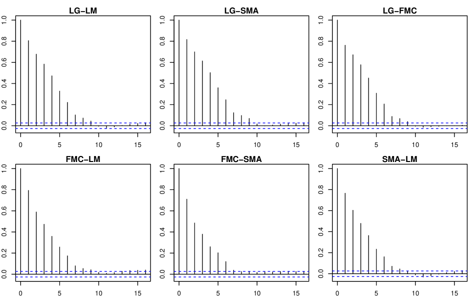
Figure S13: Sample autocorrelation function of the Poisson score differentials for the forecasts from Table 1 in the main paper, with lag in days

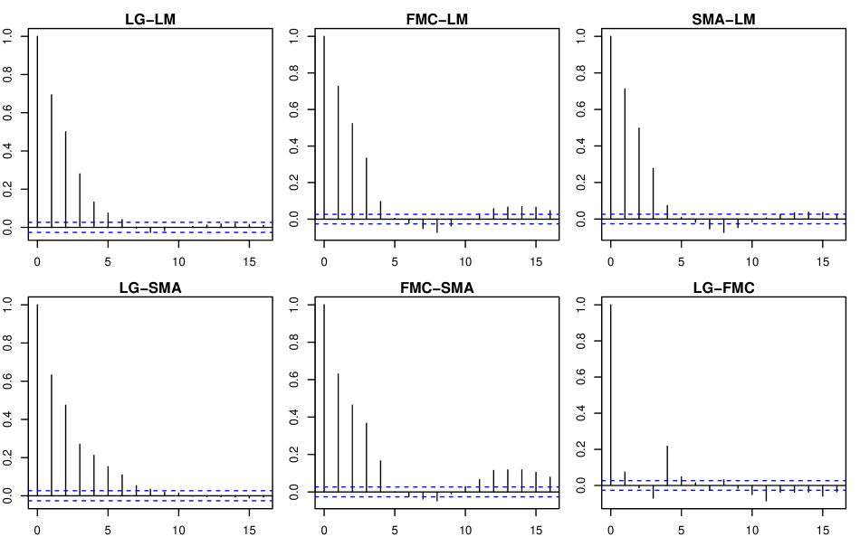
Figure S14: Same as Figure S13, but under the quadratic score

References

- Baddeley and Turner, (2005) Baddeley, A., Turner, R. (2005). spatstat: An R package for analyzing spatial point patterns. Journal of Statistical Software, 12, 1–42.
- Baddeley et al., (2005) Baddeley, A., Turner, R., Møller, J., Hazelton, M. (2005). Residual analysis for spatial point processes. Journal of the Royal Statistical Society Series B: Statistical Methodology, 67, 617–666.
- Baddeley et al., (2015) Baddeley, A., Rubak, E., Turner, R. (2015). Spatial Point Patterns: Methodology and Applications with R. Chapman and Hall/CRC Press, London.
- Bray and Schoenberg, (2013) Bray, A., Schoenberg, F. P. (2013). Assessment of point process models for earthquake forecasting. Statistical Science, 28, 510–520.
- Bray et al., (2014) Bray, A., Wong, K., Barr, C. D., Schoenberg, F. P. (2014). Voronoi residual analysis of spatial point process models with applications to California earthquake forecasts. Annals of Applied Statistics, 8, 2247–2267.
- Brehmer, (2021) Brehmer, J. R. (2021). A construction principle for proper scoring rules. Proceedings of the American Mathematical Society Series B, 8, 297–301.
- Brehmer, (2023) Brehmer, J. R. (2023). Reproduction material for “Comparative evaluation of point process forecasts”. Available at https://github.com/jbrehmer42/pp_evaluation.
- Chen et al., (2018) Chen, J., Hawkes, A. G., Scalas, E., Trinh, M. (2018). Performance of information criteria for selection of Hawkes process models of financial data. Quantitative Finance, 18, 225–235.
- Chiu et al., (2013) Chiu, S. N., Stoyan, D., Kendall, W. S., Mecke, J. (2013). Stochastic Geometry and Its Applications. John Wiley & Sons, Ltd., Chichester, third edition.
- Clements et al., (2011) Clements, R. A., Schoenberg, F. P., Schorlemmer, D. (2011). Residual analysis methods for space-time point processes with applications to earthquake forecast models in California. Annals of Applied Statistics, 5, 2549–2571.
- Daley and Vere-Jones, (2003) Daley, D. J., Vere-Jones, D. (2003). An Introduction to the Theory of Point Processes. Vol. I. Springer-Verlag, New York, second edition.
- Daley and Vere-Jones, (2004) Daley, D. J., Vere-Jones, D. (2004). Scoring probability forecasts for point processes: The entropy score and information gain. Journal of Applied Probability, 41A, 297–312.
- Dawid and Musio, (2014) Dawid, A. P., Musio, M. (2014). Theory and applications of proper scoring rules. Metron, 72, 169–183.
- Dawid and Sebastiani, (1999) Dawid, A. P., Sebastiani, P. (1999). Coherent dispersion criteria for optimal experimental design. Annals of Statistics, 27, 65–81.
- Diebold and Mariano, (1995) Diebold, F. X., Mariano, R. S. (1995). Comparing predictive accuracy. Journal of Business & Economic Statistics, 13, 253–263.
- Ehm et al., (2016) Ehm, W., Gneiting, T., Jordan, A., Krüger, F. (2016). Of quantiles and expectiles: consistent scoring functions, Choquet representations and forecast rankings. Journal of the Royal Statistical Society Series B: Statistical Methodology, 78, 505–562.
- Falcone et al., (2010) Falcone, G., Console, R., Murru, M. (2010). Short-term and long-term earthquake occurrence models for Italy: ETES, ERS and LTST. Annals of Geophysics, 53, 41–50.
- Field, (2007) Field, E. H. (2007). Overview of the working group for the development of regional earthquake likelihood models (RELM). Seismological Research Letters, 78, 7–16.
- Flaxman et al., (2019) Flaxman, S., Chirico, M., Pereira, P., Loeffler, C. (2019). Scalable high-resolution forecasting of sparse spatiotemporal events with kernel methods: A winning solution to the NIJ “Real-Time Crime Forecasting Challenge”. Annals of Applied Statistics, 13, 2564–2585.
- Frongillo and Kash, (2015) Frongillo, R., Kash, I. A. (2015). Vector-valued property elicitation. Journal of Machine Learning Research: Workshop and Conference Proceedings, 40, 1–18.
- Frongillo and Kash, (2021) Frongillo, R., Kash, I. A. (2021). Elicitation complexity of statistical properties. Biometrika, 108, 857–879.
- Gerstenberger et al., (2005) Gerstenberger, M. C., Wiemer, S., Jones, L. M., Reasenberg, P. A. (2005). Real-time forecasts of tomorrow’s earthquakes in California. Nature, 435, 328–331.
- Gneiting, (2011) Gneiting, T. (2011). Making and evaluating point forecasts. Journal of the American Statistical Association, 106, 746–762.