Systematic KMTNet Planetary Anomaly Search, Paper I: OGLE-2019-BLG-1053Lb, A Buried Terrestrial Planet

Abstract

In order to exhume the buried signatures of “missing planetary caustics” in the KMTNet data, we conducted a systematic anomaly search to the residuals from point-source point-lens fits, based on a modified version of the KMTNet EventFinder algorithm. This search reveals the lowest mass-ratio planetary caustic to date in the microlensing event OGLE-2019-BLG-1053, for which the planetary signal had not been noticed before. The planetary system has a planet-host mass ratio of $q=(1.25\pm 0.13)\times 10^{-5}$. A Bayesian analysis yields estimates of the mass of the host star, $M_{\rm host}=0.61_{-0.24}^{+0.29}~{}M_{\odot}$, the mass of its planet, $M_{\rm planet}=2.48_{-0.98}^{+1.19}~{}M_{\earth}$, the projected planet-host separation, $a_{\perp}=3.4_{-0.5}^{+0.5}$ au, and the lens distance of $D_{\rm L}=6.8_{-0.9}^{+0.6}$ kpc. The discovery of this very low mass-ratio planet illustrates the utility of our method and opens a new window for a large and homogeneous sample to study the microlensing planet-host mass-ratio function down to $q\sim 10^{-5}$.

1 Introduction

The structure of the caustics plays a central role in the phenomenology of planetary microlensing light curves and thus the detectability of microlensing planets. A source must transit or come close to a caustic to create a detectable signal (Mao & Paczynski, 1991; Gould & Loeb, 1992; Gaudi, 2012). Planetary companions to microlensing hosts induce three classes of caustic structures: central, planetary and resonant caustics. For $s>s_{w}$ or $s<s_{c}$, where $s$ is the planet-host separation in units of the Einstein radius $\theta_{\rm E}$, $s_{w}\simeq 1+3q^{1/3}/2$, $s_{c}\simeq 1-3q^{1/3}/4$ and $q$ is the planet-host mass ratio (Dominik, 1999), the caustic structure consists of a small quadrilateral caustic near the host (central caustic) and one quadrilateral (for $s>s_{w}$) or two triangular (for $s<s_{c}$) caustics separated from the host position by $|s-s^{-1}|\theta_{\rm E}$ (planetary caustics). For $s_{c}<s<s_{w}$, the central and planetary caustics merge together and form a 6-sided “resonant” caustic near the host. Yee et al. (2021) showed that “near-resonant” caustics, which have boundaries ($-3\log s_{c},1.8\log s_{w}$), are as sensitive as resonant caustics due to their long magnification ridges (or troughs) extending from the central caustic and the planetary caustics. For a clear definition, we refer to caustics out of the near-resonant range as “pure-planetary” caustics.

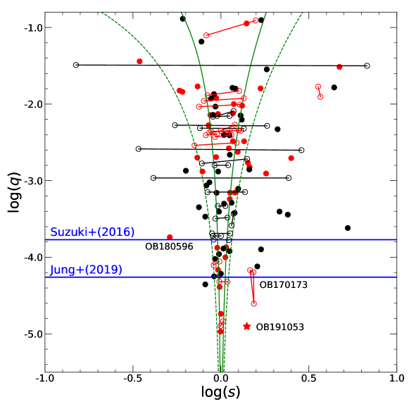
Figure 1: Microlensing parameters $(\log s,\log q)$ for planetary events, adapted from Figure 11 of Yee et al. (2021). The black and red points represent planets detected with and without KMTNet data, respectively. The red asterisk is the planet OGLE-2019-BLG-1053Lb found by the systematic search presented in this paper. Solutions are considered to be “unique” (filled points) if there are no competing solutions within $\Delta\chi^{2}<10$. Otherwise, they are shown by pairs of open circles linked by a line segment. There are eight such pairs for which $q$ differs by more than a factor of two. Seven of these are excluded on the grounds that $q$ is not accurately measured, but OGLE-2017-BLG-0173 (Hwang et al., 2018) is preserved because it was detected by a channel of pure-planetary caustic and all of its degenerate solutions have $\log q<-4$. The three $\log q<-3$ planets detected with KMTNet data are marked with text. The power-law “breaks” proposed by Suzuki et al. (2016) and Jung et al. (2019b) are indicated with the blue lines. The two green solid lines represent the boundaries between resonant and non-resonant caustics using the Equation (59) of Dominik (1999), and the two green dashed lines show the boundaries for “near-resonant” caustics proposed by Yee et al. (2021).

Although resonant and near-resonant caustics occupy a relatively narrow range of $s$, more than 80 of microlensing planets were detected via these two classes of caustics, while only 25 microlensing planets were discovered by “pure-planetary” caustics. See the $\log q$ vs. $\log s$ plot for the 114 published microlensing planets in Figure 1. Besides the high intrinsic sensitivity of resonant and near-resonant caustics, detection bias plays an important role. For many years (beginning with the second microlens planet, OGLE-2005-BLG-071Lb, Udalski et al. 2005), $\gtrsim 2/3$ of microlensing planets (see Figure 10 of Mróz et al. 2017a) were discovered based on the two-step approach advocated by Gould & Loeb (1992). In the first step, because the typical Einstein timescale $t_{\rm E}$ for microlensing events is about $20$ days (Mróz et al., 2017b), a wide-area survey with a cadence of $\Gamma\sim 1~{}{\rm day}^{-1}$ is sufficient to find microlensing events. In the second step, individual events found in the first step would be monitored by high-cadence follow-up observations from a broadly distributed network, in order to characterize the planetary signal (Albrow et al., 1998; Gould et al., 2010; Tsapras et al., 2009; Dominik et al., 2010). Due to the scarcity of telescope resources and the fact that the peak of an event can usually be predicted in advance, follow-up observations were most successful when they focused on the peak of high-magnification events, for which the source trajectory goes close to the host. Because of the large caustic size and the long magnification ridges near the host, sources of high-magnification events frequently intersect resonant and near-resonant caustics, and this explains the high frequency of microlensing planets detected through this channel. In the non-resonant case, in which the central and planetary caustics are well detached, the size of the central caustic scales as $\propto s^{2}$ for $s<1$ and $\propto s^{-2}$ for $s>1$ (Chung et al., 2005), which requires dense coverage over the peak of very-high-magnification (and therefore rare) events to capture the planetary signal, and thus only six such planets have been detected via this channel.

For the broad range of pure-planetary caustics, random source trajectories intersect the planetary caustic(s) much more often than the central caustic. For $s>1$, the ratio between the size of planetary/central caustics is $\sim q^{-1/2}$ (Han, 2006), and hence the planetary caustic is about 100 times larger than the central caustic for the common $q\sim 10^{-4}$ planets (e.g., Beaulieu et al., 2006). For $s<1$, the ratio is $\sim 0.3q^{-1/2}s$ (Han, 2006), and hence the two planetary caustics are an order of 10 times larger than the central caustic for $q\sim 10^{-4}$. Thus, the planetary caustic can play an important role in microlensing planet detections, especially for low mass-ratio planets, provided that high-cadence observations for the whole light curves can be conducted. The Microlensing Observations in Astrophysics (MOA, one 1.8 m telescope equipped with a 2.4 ${\rm deg}^{2}$ camera at New Zealand, Sumi et al. 2016) and the Optical Gravitational Lensing Experiment (OGLE, one 1.3 m telescope equipped with a 1.4 ${\rm deg}^{2}$ camera at Chile, Udalski et al. 2015) were the first to cover wide areas with high cadences of $\Gamma=1-4~{}{\rm hr}^{-1}$, which enables the detection of both microlensing events and microlensing planets without the need for follow-up observations for many events. The detection rate of pure-planetary caustics rapidly increased with the upgrades of the OGLE and MOA experiments, including the lowest mass-ratio planet prior to 2018, OGLE-2013-BLG-0341Lb with $q=(4.43\pm 0.029)\times 10^{-5}$ (Gould et al., 2014).

The new-generation microlensing survey, the Korea Microlensing Telescope Network (KMTNet, Kim et al. 2016), consists of three 1.6 m telescopes equipped with $4~{}{\rm deg}^{2}$ cameras at the Cerro Tololo Inter-American Observatory (CTIO) in Chile (KMTC), the South African Astronomical Observatory (SAAO) in South Africa (KMTS), and the Siding Spring Observatory (SSO) in Australia (KMTA). Beginning in 2016, KMTNet conducted near-continuous observations for a total area of about $100~{}{\rm deg}^{2}$ toward the Galactic bulge, with about $12~{}{\rm deg}^{2}$ at a high cadence of $\Gamma\sim 4~{}{\rm hr}^{-1}$, and about $28~{}{\rm deg}^{2}$ at a high cadence of $\Gamma\sim 1~{}{\rm hr}^{-1}$. The enhanced observational cadence of the KMTNet survey resulted in the great increase of the planet detection rate, and the microlensing planets detected with the KMTNet data comprise about half of all published planets despite of its short period of operation (see the red points in Figure 1).

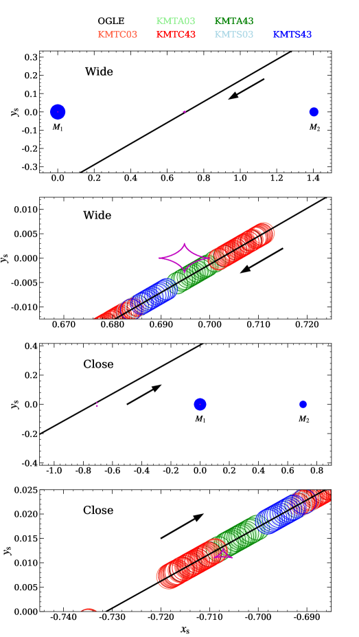
Figure 4: Geometries of the 2L1S Wide and Close models. In each panel, the magenta lines represent the caustic structure, the black solid line is the trajectory of the source, and the arrow indicates the direction of the source motion. The open circles with different colors represent the source location at the times of observation from different telescopes. The radii of the circles represent the best-fit source radius $\rho$. The blue dots, marked by $M_{1}$ (host) and $M_{2}$ (planet) are the positions of the two components of the lens.

Zhu et al. (2014) simulated a KMTNet-like survey and found that more than half of KMT $q<10^{-4}$ planets should be detected via the channel of pure-planetary caustics (see their Figure 4). In contrast to this prediction, the KMT planets detected through the channel of pure-planetary caustics comprise a minor fraction of all planet sample. Here we define this discrepancy as “missing planetary caustics” problem. Among the 14 KMT $q<10^{-3}$ planets, only two were detected by pure-planetary caustics, OGLE-2018-BLG-0596Lb (Jung et al., 2019a) with $q\sim 2\times 10^{-4}$ and OGLE-2017-BLG-0173Lb with $q\sim(2~{}{\rm or}~{}6)\times 10^{-5}$ (Hwang et al., 2018). Among the 29 $q<10^{-3}$ planets without KMT data, eight have pure-planetary caustics, while follow-up observations on high-magnification events played an important role in the detections of resonant and near-resonant caustics (e.g., Gould et al., 2006)

The “missing planetary caustics” in the KMT $q<10^{-3}$ planet sample could be due to the way that we search for planetary signals. Although KMTNet + OGLE + MOA conduct high-cadence observations over the whole microlensing season, the systematic search for planetary signals has not been extended to the light curves of whole events. For most events, modelers only search for anomalies by a visual inspection of the light curve, with their main attention devoted to the peak. For high-magnification events which are intrinsically more sensitive to planets, modelers may carefully check the observed data of the peak and the residuals from a point-source point-lens (PSPL, Paczyński 1986) fit (e.g., Jung et al., 2020; Han et al., 2021), and even trigger tender-loving care (TLC) re-reductions (e.g., Han et al., 2020a). However, the signals of $q<10^{-3}$ planetary caustics generally occur on the wings of light curves, with low amplitudes and large photometric uncertainties, and thus could have been missed due to human bias (i.e., focus on the near-peak region).

In order to find the “missing planetary caustics”, we conducted a systematic anomaly search to the whole annual light curve. We applied a modified version of the KMT EventFinder algorithm (Kim et al., 2018a) to the residuals from PSPL fits and found the lowest mass-ratio planetary caustic to date in the event OGLE-2019-BLG-1053, with $q=(1.25\pm 0.13)\times 10^{-5}$.

The paper is structured as follows. In Section 2, we describe the basic algorithm and procedures for the anomaly search. We then introduce the observations, the light-curve analysis and the physical parameters of OGLE-2019-BLG-1053 in Sections 3, 4 and 5, respectively. Finally, we discuss the implications of our work in Section 6.

2 Anomaly Search

2.1 Basic Algorithm

Normally, an anomaly in a microlensing curve refers to a deviation from a PSPL model, which could be of astrophysical origin such as an additional lens (2L1S, Mao & Paczynski 1991), an additional source (1L2S, Griest & Hu 1992) or finite-source effects (Gould, 1994; Witt & Mao, 1994; Nemiroff & Wickramasinghe, 1994), or caused by artifacts. For most microlensing planetary events, the planet-mass companion only induces several-hour to several-day deviations to a PSPL model, and the residuals from a PSPL model fit a zero-flux flat curve with short-lived deviations in some places. Thus, our basic idea is to search for such short deviations from the residuals to a PSPL model.

Shvartzvald et al. (2016) first applied an anomaly search algorithm to real complete light curves (OGLE + MOA + Wise). They calculated local $\chi^{2}$ for every 40 points and select an anomaly if a local $\chi^{2}$ exceeds a threshold. However, this algorithm does not consider the correlations in the residuals induced by by real anomalies, and it results in many false positives due to the systematics of KMT end-of-year-pipeline light curves. Thus, we apply the KMT EventFinder algorithm (Kim et al., 2018a) for the anomaly search. The KMT EventFinder adopts a Gould (1996) 2-dimensional (2D) grid of $(t_{0},t_{\rm eff})$ to search for microlensing events in the KMT end-of-year-pipeline light curves, where $t_{\rm eff}=u_{0}t_{\rm E}$ is the effective timescale, $t_{0}$ is the time of the maximum magnification, $u_{0}$ is the impact parameter in units of the angular Einstein radius $\theta_{\rm E}$, and $t_{\rm E}$ is the Einstein radius crossing time (Paczyński, 1986). It uses two approaches to fit the observed flux, $F(t)$,

$$F(t)=f_{1}A_{j}[Q(t;t_{0},t_{\rm eff})]+f_{0};\qquad Q(t;t_{0},t_{\rm eff})\equiv 1+\biggl{(}\frac{t-t_{0}}{t_{\rm eff}}\biggl{)}^{2};\qquad(j=0,1)$$ (1)

where

$$A_{j=0}(Q)=Q^{-1/2};\qquad A_{j=1}(Q)=\frac{Q+2}{\sqrt{Q(Q+4)}}=[1-(Q/2+1)^{-2}]^{-1/2},$$ (2)

and ($f_{1},f_{0}$) are two flux parameters, which are evaluated by a linear fit.

In reality, the planetary deviations are not simply symmetric single “bumps” except for events that consist of two isolated PSPL curves that are respectively caused by the host and a wide-orbit planet (e.g., Han et al., 2017), so our search model cannot fit the deviations perfectly. However, the main purpose of the 2D grid search is to locate the signal and roughly estimate its significance. For a signal that passes the EventFinder threshold, the KMT EventFinder pipeline further fits it with a PSPL model and evaluates it with a second threshold (Kim et al., 2021a). Given an acceptable level of effort to carry out a manual review with low-threshold candidates (see Section 2.5 and 6.2), it is unnecessary to design models that perfectly fit the light curve, which would actually be very difficult due to the diversity of deviations. In addition, the deviations contain not only “bumps”, which are the targets of the EventFinder, but also “dips” (e.g., Gould et al., 2014) and “U shapes”, which are caused by caustic crossings (e.g., Bond et al., 2004). Nevertheless, “dips” can be regarded as the inverse of “bumps” and be fitted by a negative $f_{1}$, while each peak of “U shapes” or even the whole “U shapes” can be regarded as a bump, as shown in Figure 11 of Kim et al. (2018a).

2.2 Data Handling

KMTNet made end-of-year-pipeline light curves public for the 2015–2019 seasons. We adopt the events from the 2019 season, because its light-curve files contain seeing and sky background information. This auxiliary information provides a systematic way to exclude most of the bad points which frequently generate fake signals. Based on an investigation of bad points, we exclude data points that have a sky background brighter than $5000$ ADU/pixel or a seeing FWHM larger than 7 pixels ($0.4^{\prime\prime}$ per pixel) for the KMTA and KMTS data and 6.5 pixels for the KMTC data. We also exclude KMTS data between ${\rm HJD}^{\prime}$ = 8640 – 8670 (${\rm HJD}^{\prime}={\rm HJD}-2450000$) on CCD N chip, which have anomalous fluxes due to a failing electrical connection in that chip.

In general, the errors from photometric measurements for each data set $i$ were renormalized using the formula $\sigma_{i}^{\prime}=k_{i}\sqrt{\sigma_{i}^{2}+e^{2}_{i,{\rm min}}}$, where $\sigma_{i}$ and $\sigma_{i}^{\prime}$ are the original error bars from the photometry pipelines and the renormalized error bars in magnitudes, and $k_{i}$ and $e_{i,{\rm min}}$ are rescaling factors. The rescaling factors are often determined using the method of Yee et al. (2012), which enables $\chi^{2}/{\rm dof}$ for each data set to become unity. However, this procedure is not feasible for our search. For the PSPL fits, the error bars were overestimated, because some outliers have not been excluded by the seeing and sky background thresholds, and the data cannot fit a PSPL model if an event includes an anomaly. For the anomaly search to the residuals, because our search model cannot fit the deviations perfectly, it is unreasonable to require $\chi^{2}/{\rm dof}=1$. Thus, we simply adopt $k=1.5$ and $e_{\rm min}=0$ for each data set, after an investigation of the rescaling factors of error bars for a subset of PSPL events.

Finally, the pipeline data, which are in the magnitude units, are converted to the flux unit using the same $(I=28)$ zero point that was used by the KMT end-of-year pipeline.

2.3 Event Selection

We adopt the $I_{\rm cat}<19.0$ events as our first sample (1216 in total), where $I_{\rm cat}$ is the star-catalog magnitude entry in the KMT database. For regions covered by the OGLE-III catalog (Szymański et al., 2011), we adopt the $I_{\rm cat}$ value from the OGLE-III catalog. For most regions that are not covered by OGLE-III, $I_{\rm cat}$ is taken as the $i^{\prime}$ magnitude from the catalog of Schlafly et al. (2018) derived from DECam data. For the small regions not covered by either catalog, $I_{\rm cat}$ is derived from DoPHOT (Schechter et al., 1993) reductions of the KMT templates. For each event, the KMT end-of-year-pipeline adopts $I_{\rm cat}$ as the baseline magnitude of light curves, which includes both the source flux and the blended light. There are two reasons for this brightness threshold. First, the main purpose of the current search is to develop and test the method and programming, which requires repeated computation and manual review. To ease the burden, it is necessary to select a small but sensitive sample. Second, because the signals of planetary caustics often occur on the wings of the light curves and the $I\geq 19.0$ data have large photometric uncertainties, it is difficult (but not impossible, e.g., Zhang et al. 2020) to find planetary signals from the $I\geq 19.0$ data. A more comprehensive approach may be to adopt all of the $I<19.0$ data, rather than selecting only $I_{\rm cat}<19.0$ events, but the current sample is sufficient for the main purpose of our search. We will discuss further improvements to our search in Section 6.2.

We fit the 1216 $I_{\rm cat}<19.0$ events with the PSPL model by a downhill approach using ($t_{0},u_{0},t_{\rm E}$) from the KMT website as the initial parameters. We then manually review the PSPL model plots and find that 219 events have either an obvious variable source, too low signal-to-noise ratios of the microlensing effects, very noisy photometry for all of the data sets, or are of non-microlensing origins (e.g., cataclysmic variables). We remove these events. For the remaining 997 events, we photometrically align the PSPL residuals of each data set to the KMTC or KMTS residuals using the two flux parameters, ($f_{1},f_{0}$), from the PSPL fits.

2.4 Detailed Search

The set of $t_{{\rm eff},k}$ are a geometric series,

$$t_{{\rm eff},k+1}=(4/3)t_{{\rm eff},k},$$ (3)

with the shortest effective timescale $t_{{\rm eff},1}=0.30$ days and the longest effective timescale $t_{{\rm eff},13}=0.30\times(4/3)^{12}=9.47$ days. Here $t_{{\rm eff},1}=0.30$ is adopted from the current lower limit of $t_{\rm eff}$ of the KMT EventFinder pipeline (Kim et al., 2021a). While $t_{\rm eff}\gtrsim 5$ days is definitely too long for planetary signals, we consider that some short-timescale events could be caused by a wide-orbit planet (e.g., Han et al., 2020b), so the series of long $t_{\rm eff}$ are designed for the weak signals of a possible host star. The step size of $t_{0}$ is $\delta_{t_{0}}=(1/6)t_{\rm eff}$, and the grids begin at $\delta_{t_{0}}$ before the first epoch of the 2019 season and end at $\delta_{t_{0}}$ after the last epoch. We restrict the search at each grid point ($t_{0},t_{\rm eff}$) to data within $t_{0}\pm 3~{}t_{\rm eff}$ and require that this interval contains at least five data points and at least three successive points $\geq 2\sigma$ away from the zero-residual curve.

Finally, each grid point is evaluated by two parameters, $\Delta\chi^{2}_{\rm zero}$ and $\Delta\chi^{2}_{\rm flat}$,

$$\Delta\chi^{2}_{\rm zero}=\chi^{2}_{\rm zero}-\chi^{2}_{\rm signal};\qquad\Delta\chi^{2}_{\rm flat}=\chi^{2}_{\rm flat}-\chi^{2}_{\rm signal},$$ (4)

where $\chi^{2}_{\rm zero}$, $\chi^{2}_{\rm flat}$ and $\chi^{2}_{\rm signal}$ are the $\chi^{2}$ to the zero-flux curve, the mean-flux curve, and the search model, respectively, $\Delta\chi^{2}_{\rm zero}$ determines the significance of the signal, and $\Delta\chi^{2}_{\rm flat}$ characterizes the steepness of the residual flux. For most signals, such as clear “bumps” or “dips”, both $\Delta\chi^{2}_{\rm zero}$ and $\Delta\chi^{2}_{\rm flat}$ are significant. However, for some long-$t_{\rm eff}$ signals that are caused by long-term variability or systematics, $\Delta\chi^{2}_{\rm flat}\sim 0$. After reviewing some recognized signals with different $\Delta\chi^{2}_{\rm zero}$ and $\Delta\chi^{2}_{\rm flat}$, we decide to select if (1) $\Delta\chi^{2}_{\rm zero}>120$; or (2) $\Delta\chi^{2}_{\rm zero}>75$ and $\Delta\chi^{2}_{\rm flat}>35$. After reviewing some recognized signals, we find that in average $\chi^{2}_{\rm 1L1S}-\chi^{2}_{\rm 2L1S}\sim 1.6$ $\Delta\chi^{2}_{\rm zero}$. Taking into account that it could require $\chi^{2}_{\rm 1L1S}-\chi^{2}_{\rm 2L1S}\sim 120$ to ensure a real detection and the efforts required for manual review, we decide to select if (1) $\Delta\chi^{2}_{\rm zero}>120$; or (2) $\Delta\chi^{2}_{\rm zero}>75$ and $\Delta\chi^{2}_{\rm flat}>35$. Two signals (A, B) from the same event are judged to be the same signal provided that $|t_{0,{\rm A}}-t_{0,{\rm B}}|<t_{\rm eff,A}+t_{\rm eff,B}$. As a result, the anomaly search yielded 6320 candidate signals from 422 events.

2.5 Manual Review and Results

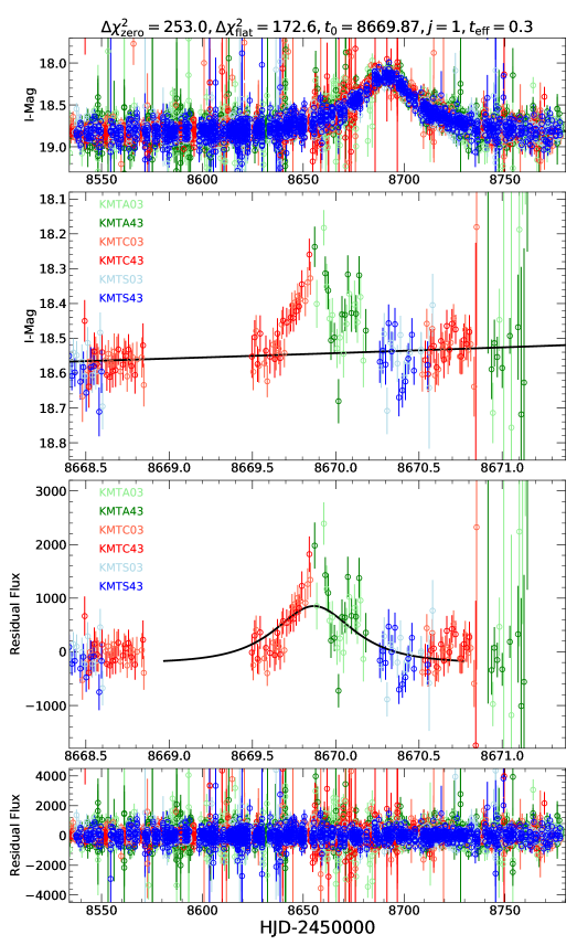
Figure 2: Example of the candidate signal of OGLE-2019-BLG-1053 (ultimately judged to be real) as shown to the operator. The first and fourth panels show the whole season of data and their residuals to the PSPL model, respectively. The second and third panels show a zoom ($t_{0}\pm 5~{}t_{\rm eff}$) of the candidate signal. The circles with different colors are observed data points for different data sets. The black line in the second panel represents the best-fit PSPL model, and the black line in the third panel represents the best-fit grid-search model for $t_{0}\pm 3~{}t_{\rm eff}$. Five parameters are shown above the first panel: $\Delta\chi^{2}_{\rm zero}$, $\Delta\chi^{2}_{\rm flat}$, $t_{0}$, $j$ and $t_{\rm eff}$.

Each candidate is shown to the operator in a four-panel display together with some auxiliary information. The display shows the light curves and residuals for the signal and for the data of the whole season. See Figure 2 for an example. For candidates that are assessed as plausibly real (i.e., not an artifact), the operator first checks whether the event was independently found by OGLE and/or MOA, and if so whether their on-line light curves have data points during the anomaly. If they do, and if these data points are inconsistent with the KMT-based anomaly, the candidate is rejected. For example, for KMT-2019-BLG-0607/OGLE-2019-BLG-0667, the KMTC data shows a $\sim 0.3$-day bump on the peak, but the OGLE data do not show this bump. If no such external check is possible, then the anomaly is investigated by a variety of techniques at the image level before proceeding to the next step. For example, for KMT-2019-BLG-2418, a long, low-amplitude bump was found about 120 days before the $t_{\rm E}\sim 4$-day short event that had previously been selected as a microlensing event. The bump appeared in all three KMT data sets, and so could have represented a “host” to the short-event “planet”. Neither OGLE nor MOA had found a counterpart to this event. However, investigation of the images showed that the bump was due to flux from a nearby variable, so the candidate was rejected.

As a result, the operator (W. Zang) identified 24 candidates that could be planetary events and 59 candidates that should be other types of anomaly (e.g., binary-star events). Among the 24 candidate planets, four are known planets (e.g., Yee et al., 2021) and four are finite-source point-lens events (Kim et al., 2021a). For the remaining 16 candidates, preliminary 2L1S fits suggested that OGLE-2019-BLG-1053 has a pure-planetary caustic induced by a very low mass-ratio planet. This triggered TLC re-reductions for the KMT data, which combined with the OGLE data on the anomaly, revealed a clear planetary signal.

3 Observations of OGLE-2019-BLG-1053

On 5 July 2019, OGLE-2019-BLG-1053 was announced as a microlensing candidate event by the OGLE Early Warning System (Udalski et al., 1994; Udalski, 2003) at equatorial coordinates $(\alpha,\delta)_{\rm J2000}$ = (18:00:39.93, $-27$:20:29.7), corresponding to Galactic coordinates $(\ell,b)=(3.06,-2.05)$. It was then independently discovered by the KMT alert-finder system (Kim et al., 2018b) at the position of an $I=18.84$ catalog star and announced as a clear microlensing candidate KMT-2019-BLG-1504 on 7 July 2019.

The OGLE observations were carried out using the 1.3 m Warsaw Telescope equipped with a 1.4 ${\rm deg}^{2}$ FOV mosaic CCD camera at the Las Campanas Observatory in Chile (Udalski et al., 2015). The event lies in the OGLE BLG511 field, with a cadence of $\Gamma=1~{}{\rm hr}^{-1}$. The event lies in two slightly offset KMT fields, BLG03 and BLG43, with a combined cadence of $\Gamma\sim 4~{}{\rm hr}^{-1}$.

For both surveys, most images were taken in the $I$ band, and a fraction of images were taken in the $V$ band for the source color measurements. In addition, This event was also observed by the Spitzer space telescope. We discuss those observations in Appendix § A.

The ground-based data used in the light curve analysis were reduced using custom implementations of the difference image analysis technique (Tomaney & Crotts, 1996; Alard & Lupton, 1998): Wozniak (2000) for the OGLE data and pySIS (Albrow et al., 2009) for the KMT data. For the KMTC03 data, we conduct pyDIA photometry to measure the source color. The $I$-band magnitude of the data has been calibrated to the standard $I$-band magnitude using the OGLE-III star catalog (Szymański et al., 2011). The errors from photometric measurements for each data set were readjusted following the routine of Yee et al. (2012). The data used in the analysis, together with the corresponding data reduction method and the rescaling factors are summarized in Table 1.

4 Light-curve Analysis

4.1 Heuristic Analysis

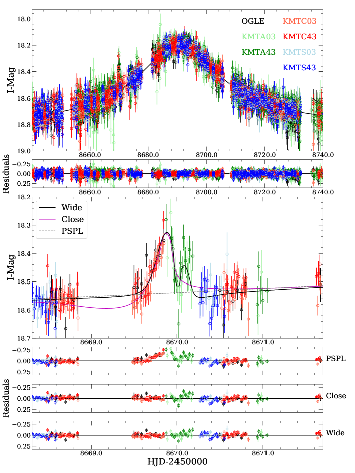
Figure 3: The observed data with the best-fit models. The open circles with different colors are observed ground-based data points for different data sets. The bottom four panels show a close-up of the planetary signal and the residuals to different models. The black and magenta solid lines represent the best-fit 2L1S Wide and Close models, respectively, and the black dashed line represents the best-fit PSPL model.

Figure 3 shows the OGLE-2019-BLG-1053 data together with the best-fit models. The light curve shows two consecutive small bumps ($t_{0,{\rm anom}}\sim 8670$) 20.5 days before the peak of an otherwise normal PSPL light curve. Such a bump is a typical signature of a planet produced by the source approach or crossing over the planetary caustic (Gould & Loeb, 1992). The 2L1S model requires three additional parameters $(s,q,\alpha)$, where $\alpha$ is the angle of the source trajectory relative to the binary axis. We also consider finite-source effects and include the source radius normalized by the Einstein radius, $\rho=\theta_{*}/\theta_{\rm E}$.

We first fit the PSPL model excluding the data points around the anomaly and obtain

$$(t_{0},u_{0},t_{\rm E})=(8690.5,0.35,34~{}{\rm days}),$$ (5)

which leads to

$$\tau_{\rm anom}=\frac{t_{\rm anom}-t_{0}}{t_{\rm E}}=-0.60;\qquad u_{\rm anom}=\sqrt{u_{0}^{2}+\tau_{\rm anom}^{2}}=0.695;\qquad|\alpha|=|\tan^{-1}\frac{u_{0}}{\tau_{\rm anom}}|=0.53~{}(30.3^{\circ}).$$ (6)

Because the planetary caustic is located at the position of $|s-s^{-1}|\sim u_{\rm anom}$, we obtain

$$s\sim\frac{\sqrt{u_{\rm anom}^{2}+4}+u_{\rm anom}}{2}=1.41~{}{\rm or}~{}s\sim\frac{\sqrt{u_{\rm anom}^{2}+4}-u_{\rm anom}}{2}=0.71.$$ (7)

For the remaining two 2L1S parameters, $q$ and $\rho$, a systematic search is required.

4.2 Numerical Analysis

We use the advanced contour integration code (Bozza, 2010; Bozza et al., 2018) VBBinaryLensing to calculate the magnification of the 2L1S model. We locate the $\chi^{2}$ minima by conducting a grid search over the parameter plane ($\log s,\log q,\alpha$). The grid consists of 21 values equally spaced between $-0.2\leq\log s\leq 0.2$, 10 values equally spaced between $0^{\circ}\leq\alpha<360^{\circ}$, and 61 values equally spaced between $-6\leq\log q\leq 0$. For each set of ($\log s,\log q,\alpha$), we fix $\log q$, $\log s$ and let the other parameters ($t_{0},u_{0},t_{\rm E},\rho,\alpha$) vary. We find a lensing solution using the Markov chain Monte Carlo (MCMC) $\chi^{2}$ minimization applying the emcee ensemble sampler (Foreman-Mackey et al., 2013). From this, we find two distinct minima with ($\log s,\log q)\sim$ ($-0.15,-4.5$) and ($0.15,-4.9$) and label them by “Close” ($s<1$) and “Wide” ($s>1$) in the following analysis. We then investigate the best-fit models with all free parameters. The best-fit parameters with their $68\%$ uncertainty range from the MCMC are shown in Table 2, and the caustics and source trajectories are shown in Figure 4. We note that the heuristic estimates for $(s,\alpha)$ are in good agreement with the values in Table 2.

We found that the Wide model provides the best fit to the observed data, and the $\chi^{2}$ improvement to the best-fit PSPL model is 453.6. The two consecutive small bumps are produced by the source crossing the two spikes of the quadrilateral caustic. The Close model is disfavored by $\Delta\chi^{2}=41.6$, and all of the $\chi^{2}$ difference come from the anomalous region. We also check whether the $\Delta\chi^{2}$ can be decreased by considering the microlens ground-based parallax effect (Gould, 1992, 2000, 2004), which is caused by the orbital acceleration of Earth, and the lens orbital motion effect (Batista et al., 2011; Skowron et al., 2011), but all the Close solutions have $\Delta\chi^{2}>40$ compared to the Wide solutions and cannot reproduce the double-bump feature. Thus, we exclude the Close model and only investigate the Wide model in the following analysis. In addition, we check the 1L2S model and find that it is disfavored by $\Delta\chi^{2}>400$. Thus, we exclude the 1L2S model, too.

We check whether the fit to the wide model further improves by including the microlens ground-based parallax effect,

$$\bm{\pi}_{\rm E}=\frac{\pi_{\rm rel}}{\theta_{\rm E}}\frac{\bm{\mu}_{\rm rel}}{\mu_{\rm rel}}~{},$$ (8)

where $(\pi_{\rm rel},\bm{\mu}_{\rm rel})$ are the lens-source relative (parallax, proper motion). We parameterize the microlens parallax by $\pi_{\rm E,N}$ and $\pi_{\rm E,E}$, which are the North and East components of the microlens parallax vector. We also fit the $u_{0}>0$ and $u_{0}<0$ solutions to consider the “ecliptic degeneracy” (Jiang et al., 2004; Poindexter et al., 2005). The addition of parallax to the model only improves $\Delta\chi^{2}\leq 1.2$ (see Table 2), but it provides “1-D parallax” constraint with $\sigma(\pi_{\rm E,\parallel})\sim 0.05$, where $\pi_{\rm E,\parallel}$ is the component of $\bm{\pi}_{\rm E}$ that in the direction of the projected position of the Sun at $t_{0}$. We also consider the lens orbital motion effect and find that it is not detectable ($\Delta\chi^{2}<0.3$) and not correlated with $\bm{\pi}_{\rm E}$, so we eliminate the lens orbital motion from the fit.

5 Lens Properties

5.1 Color Magnitude Diagram

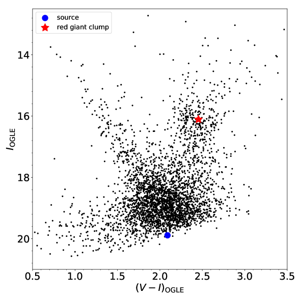
Figure 5: Color-magnitude diagram (CMD) for field stars within $80^{\prime\prime}$ centered on OGLE-2019-BLG-1053 using the OGLE-III star catalog (Szymański et al., 2011). The red asterisk and blue dot represent the positions of the centroid of the red giant clump and the microlensing source star, respectively.

We estimate the intrinsic brightness and color of the source by locating the source on a color magnitude diagram (CMD) (Yoo et al., 2004). We construct a $V-I$ versus $I$ CMD using the OGLE-III catalog stars (Szymański et al., 2011) within $80^{\prime\prime}$ centered on the event (see Figure 5). We measure the centroid of the red giant clump as $(V-I,I)_{\rm cl}=(2.45\pm 0.01,16.11\pm 0.02)$ and adopt the intrinsic color and de-reddened magnitude of the red giant clump $(V-I,I)_{\rm cl,0}=(1.06,14.35)$ from Bensby et al. (2013) and Nataf et al. (2013). For the source color, we obtain $(V-I)_{\rm S}=2.09\pm 0.03$ by regression of the KMTC03 $V$ versus $I$ flux with the change of the lensing magnification and a calibration to the OGLE-III magnitudes. Using the color/surface-brightness relation for dwarfs and subgiants of Adams et al. (2018), we obtain

$$\theta_{*}= 0.762\pm 0.053~{}\mu{\rm as}~{}{\rm for~{}the}~{}u_{0}>0~{}{\rm solution},$$ (9)

$$\theta_{*}= 0.759\pm 0.053~{}\mu{\rm as}~{}{\rm for~{}the}~{}u_{0}<0~{}{\rm solution}.$$ (10)

5.2 Bayesian Analysis

For a lensing object, the total mass $M_{\rm L}$ and the lens distance $D_{\rm L}$ are related to the angular Einstein radius $\theta_{\rm E}$ and the microlens parallax $\pi_{\rm E}$ by (Gould, 1992, 2000)

$$M_{\rm L}=\frac{\theta_{\rm E}}{{\kappa}\pi_{\rm E}};\qquad D_{\rm L}=\frac{\mathrm{au}}{\pi_{\rm E}\theta_{\rm E}+\pi_{\rm S}},$$ (11)

where $\kappa\equiv 4G/(c^{2}\mathrm{au})=8.144$ mas$/M_{\odot}$, $\pi_{\rm S}=\mathrm{au}/D_{\rm S}$ is the source parallax, and $D_{\rm S}$ is the source distance. Using the measurements of $\rho$ from the light-curve analysis and $\theta_{*}$ from the CMD analysis, we obtain the angular Einstein radius

(13)

Combined with the measurement $t_{\rm E}\sim 34$ days, these values imply a lens-source relative proper motion $\mu_{\rm rel}\sim 4~{}{\rm mas\,yr^{-1}}$. However, the observed data only give a weak constraint on the microlens parallax. We therefore conduct a Bayesian analysis based on a Galactic model to estimate the physical parameters of the planetary system.

The Galactic model mainly consists of three aspects: the mass function of the lens, the stellar number density profile and the source and lens velocity distributions. For the lens mass function, we begin with the initial mass function (IMF) of Kroupa (2001) for both the disk and the bulge. To approximate the impact of the age and vertical dispersion as a function of age of the disk population, we impose a cut off of $1.3~{}M_{\odot}$ (Zhu et al., 2017). Taking account of the age distribution of microlensed dwarfs and subgiants of Figure 13 of Bensby et al. (2017), we impose a cut off of $1.1~{}M_{\odot}$ for the bulge. For the bulge and disk stellar number density, we choose the models used by Zhu et al. (2017) and Bennett et al. (2014), respectively. For the disk velocity distribution, we assume the disk lenses follow a rotation of $240~{}{\rm km~{}s}^{-1}$ (Reid et al., 2014) with the velocity dispersion of Han et al. (2020c). For the bulge dynamical distributions, we adopt the Gaia proper motion of red giant stars within $5^{\prime}$ (Gaia Collaboration et al., 2016, 2018) and obtain

$$\langle\bm{\mu}_{\rm bulge}(\ell,b)\rangle=(-5.65,-0.09)\pm(0.15,0.11)~{}\text{masyr}^{-1},$$ (14)

$$\sigma(\bm{\mu}_{\rm bulge})=(3.15,2.54)\pm(0.17,0.13)~{}\text{masyr}^{-1}.$$ (15)

We create a sample of $10^{8}$ simulated events from the Galactic model. For each simulated event $i$ of solution $k$, we weight it by

$$\omega_{{\rm Gal},i,k}=\Gamma_{i,k}\mathcal{L}_{i,k}(t_{\rm E})\mathcal{L}_{i,k}(\theta_{\rm E})\mathcal{L}_{i,k}(\bm{\pi}_{\rm E}),$$ (16)

where $\Gamma_{i,k}\varpropto\theta_{{\rm E},i,k}\times\mu_{{\rm rel},i,k}$ is the microlensing event rate, $\mathcal{L}_{i,k}(t_{\rm E})$, $\mathcal{L}_{i,k}(\theta_{\rm E})$ and $\mathcal{L}_{i,k}(\bm{\pi}_{\rm E})$ are the likelihood of its inferred parameters $(t_{\rm E},\theta_{\rm E},\bm{\pi}_{\rm E})_{i,k}$ given the error distributions of these quantities derived from the MCMC for that solution

$$\mathcal{L}_{i,k}(t_{\rm E})=\frac{{\rm exp}[-(t_{{\rm E},i,k}-t_{{\rm E},k})^{2}/2\sigma^{2}_{t_{{\rm E},k}}]}{\sqrt{2\pi}\sigma_{t_{{\rm E},k}}},$$ (17)

$$\mathcal{L}_{i,k}(\theta_{\rm E})=\frac{{\rm exp}[-(\theta_{{\rm E},i,k}-\theta_{{\rm E},k})^{2}/2\sigma^{2}_{\theta_{{\rm E},k}}]}{\sqrt{2\pi}\sigma_{\theta_{{\rm E},k}}},$$ (18)

$$\mathcal{L}_{i,k}(\bm{\pi}_{\rm E})=\frac{{\rm exp}[-\sum_{m,n=1}^{2}b_{m,n}^{k}(\pi_{{\rm E},m,i}-\pi_{{\rm E},m,k})(\pi_{{\rm E},n,i}-\pi_{{\rm E},n,k})/2]}{2\pi/\sqrt{{\rm det}~{}b^{k}}},$$ (19)

$b_{m,n}^{k}$ is the inverse covariance matrix of $\bm{\pi}_{{\rm E},k}$, and $(m,n)$ are dummy variables ranging over ($N,E$). Finally, we combine the Bayesian result of the $u_{0}>0$ and $u_{0}<0$ solutions by their Galactic-model likelihood and ${\rm exp}(-\Delta\chi^{2}_{k}/2)$, where $\Delta\chi^{2}_{k}$ is the $\chi^{2}$ difference between the $k$th solution and the best-fit solution.

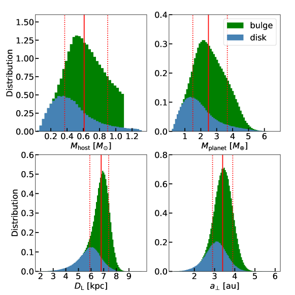
Figure 6: Bayesian posterior distributions of the lens mass $M_{\rm L}$, the planet mass $M_{\rm planet}$, the lens distance $D_{\rm L}$ and the projected planet-host separation $a_{\perp}$. The distributions are the combined results of the $u_{0}>0$ and $u_{0}<0$ solutions by their Galactic-model likelihood and ${\rm exp}(-\Delta\chi^{2}/2)$, where $\Delta\chi^{2}$ is the $\chi^{2}$ difference between the two solutions. In each panel, the red solid vertical line and the two red dashed lines represent the median value and the 15.9% and 84.1% percentages of the distribution. The total distribution is divided into bulge (green) and disk (blue) lenses. The upper limits of the host mass is $1.1~{}M_{\odot}$ for bulge lenses and $1.3~{}M_{\odot}$ for disk lenses. See Section 5.2.

The resulting posterior distributions of the host mass $M_{\rm host}$, the planet mass $M_{\rm planet}$, the lens distance $D_{\rm L}$ and the projected planet-host separation $a_{\perp}$ are listed in Table 3 and shown in Figure 6. The presented parameters are the median values of the Bayesian distributions, and the upper and lower limits correspond to the $15.9\%$ and $84.1\%$ percentages of their distributions, respectively. The Bayesian analysis yields a host mass of $M_{\rm host}=0.61_{-0.24}^{+0.29}~{}M_{\odot}$, a planet mass of $M_{\rm planet}=2.48_{-0.98}^{+1.19}~{}M_{\earth}$, a host-planet projected separation $a_{\perp}=3.4_{-0.5}^{+0.5}$ au and a lens distance of $D_{\rm L}=6.8_{-0.9}^{+0.6}$ kpc. The estimated physical parameters indicate that lens companion is a terrestrial planet located well beyond the snow line of the host star (assuming a snow line radius $a_{\rm SL}=2.7(M/M_{\odot})$ au, Kennedy & Kenyon 2008). In addition, for an $M\sim 0.6~{}M_{\odot}$ star at a distance of $\sim 6.8$ kpc, it should be behind most of the dust extinction and its apparent magnitude should be $I_{\rm L}\sim 23$. Hence, it is estimated that the lens flux only contributes a very small fraction of the $I_{\rm B}\sim 19.4$ blended light.

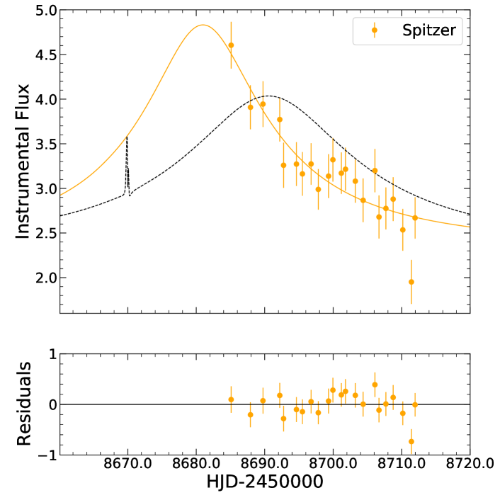
Figure 7: The observed Spitzer data (orange points) in instrumental-flux units and the best-fit Spitzer-“ONLY” model (the orange solid curve). The black dotted line represents the Spitzer flux predicted by the best-fit 2L1S model derived from the ground-based analysis for $\bm{\pi}_{\rm E}=(0,0)$ evaluated at the central value of the $VLI$ color-color constraint. The total flux change of the Spitzer light curve is $\sim 2.0$ instrumental flux unit, which is only a few times the level of systematics seen in other Spitzer events with observations in the baseline (Gould et al., 2020; Hirao et al., 2020; Zang et al., 2020).

We note that although the introduction of $\bm{\pi}_{\rm E}$ does not significantly improve the fit, it does constrain the amplitude of $\bm{\pi}_{\rm E,E}$ to be small, and thereby influences the mass estimate via Equation (11). In particular, if we remove the $\bm{\pi}_{\rm E}$ term from Equation (16), then the Bayesian host mass estimate is shifted lower to $M_{\rm host}=0.52_{-0.30}^{+0.32}~{}M_{\odot}$. We also note that this is in good agreement with the general prediction of Kim et al. (2021b), for the case of $\theta_{\rm E}=0.37$ mas and $\mu_{\rm rel}<10~{}{\rm mas\,yr^{-1}}$ (and no other information), i.e., $M_{\rm host}=0.45_{-0.23}^{+0.30}~{}M_{\odot}$. See their Figures 6 and 7.

6 Discussion

6.1 A New Path for the Mass-ratio Function

For most microlensing planetary events, light-curve analyses do not provide the masses of the host and the planet, but the planet-host mass ratio, $q$, is well determined. There have been three studies about the microlensing planet-host mass-ratio function from homogeneous samples. Gould et al. (2010) adopted the 13 high-magnification events intensively observed by the Microlensing Follow Up Network ($\mu$FUN), which included six planets. Shvartzvald et al. (2016) used the 224 events observed by OGLE + MOA + Wise Observatory, including seven $q<0.01$ planets. It confirmed the result of Sumi et al. (2010) that the planet occurrence rate increases while q decreases for $-4.5<\log q<-2.0$. Suzuki et al. (2016) built a substantially larger sample that consisted of 1474 events discovered by the MOA-II microlensing survey alert system, the Gould et al. (2010) sample and 196 events from the PLANET follow-up network (Cassan et al., 2012), with 30 planets in total. This larger sample revealed a break in the mass-ratio function at about $q_{\rm break}=17\times 10^{-5}$, below which the planet occurrence rate decreases as $q$ decreases.

KMT opens a window for the mass-ratio function down to $q\sim 10^{-5}$ and thus can test the break reported by Suzuki et al. (2016). Including OGLE-2019-BLG-1053Lb, KMT has detected five very low mass-ratio planets whose mass ratios lie below the lowest mass ratio, $q=(4.43\pm 0.029)\times 10^{-5}$ (Gould et al., 2014), in the three samples mentioned above. The four other planets are KMT-2018-BLG-0029Lb with $q\sim 1.8\times 10^{-5}$ (Gould et al., 2020), KMT-2019-BLG-0842Lb with $q\sim 4.1\times 10^{-5}$ (Jung et al., 2020), OGLE-2019-BLG-0960Lb with $q\sim 1.4\times 10^{-5}$ (Yee et al., 2021) and KMT-2020-BLG-0414Lb with $q\sim 1.1\times 10^{-5}$ (Zang et al., 2021). KMT data played a major or decisive role in all the five discoveries. However, it is challenging to build a homogeneous KMT sample, considering that there are $\sim 3000$ KMT events per year and the imperfect end-of-year-pipeline light curves. Yee et al. (2021) proposed to construct a KMT high-magnification sample by placing a magnification threshold (e.g., $A_{\rm max}>20$), but this approach would require intensive efforts on KMT TLC re-reductions. A second approach, proposed by Zang et al. (2021), is to systematically follow up high-magnification events in the KMT low-cadence ($\Gamma\lesssim 1~{}{\rm hr}^{-1}$) fields using Las Cumbres Observatory (LCO) global network and $\mu$FUN. Because the follow-up data would play a major role in the detections of planetary signals, this approach would require many fewer KMT TLC re-reductions (and so, much less effort) than the Yee et al. (2021) approach, but it would require intensive effort to carry out the real-time monitoring and obtain follow-up observations.

The anomaly search to the KMT end-of-year-pipeline light curves provides a new path for the mass-ratio function with a large and homogeneous sample. This approach would only require KMT TLC re-reductions on candidate planetary events, and most of the KMT events can be included in the sample except a small fraction of events, e.g., events with a variable source. We applied the anomaly search to the known 2019 KMT planets, and all of them were identified as a candidate signal with the current search thresholds, including the two very low mass-ratio planets, KMT-2019-BLG-0842Lb with $\Delta\chi^{2}_{\rm zero}=519$ and OGLE-2019-BLG-0960Lb with $\Delta\chi^{2}_{\rm zero}=2623$. This should hold for almost all the 2016–2019 KMT planets, and the final planet sample from the 2016–2019 data should be at least two times larger than the Suzuki et al. (2016) sample.

6.2 Future Improvements of Anomaly Search

The main purpose of the current search is to develop and test the method and programming. The detection of the lowest mass-ratio planetary caustic to date illustrates the utility of this search. The ultimate goal of our search is to form a large and homogeneous sample to study the microlensing planet-host mass-ratio function down to $q\sim 10^{-5}$. To achieve it, the current search can be improved in several respects.

First, the search could be extended to all of the 2016–2019 events without the current catalog-star brightness limit $I_{\rm cat}<19$. At present, only the 2019 data can be used, because the 2016–2018 data lack seeing and background information and the 2016–2017 end-of-year-pipeline light curves are not of sufficiently high quality.

Second, the search could adopt shorter $t_{\rm eff}$ and lower $\chi^{2}_{\rm zero}$ thresholds. The lower limit of $t_{\rm eff}$ should be reduced to $\sim 0.05$ days, in order to find the shortest signals, at least in the $\Gamma\geq 4~{}{\rm hr}^{-1}$ fields, which cover $\sim 12~{}{\rm deg}^{2}$. Estimating that 10 points are required to characterize a short anomaly, the detection threshold for these high cadence fields is $t_{\rm eff,limit}\sim(10/\Gamma)/2=0.05$ days. For the planetary signal of OGLE-2019-BLG-1053, its best-fit has $t_{\rm eff}\sim 0.1$ days, with $\Delta\chi^{2}=49$ better than the model with $t_{\rm eff}=0.3$ days. The disadvantage is that decreasing the lower limit of $t_{\rm eff}$ leads to many more anomaly candidate signals that must be reviewed by the operator. Using $t_{{\rm eff},1}=0.05$ days, and $\Delta\chi^{2}_{\rm zero}=50$ and $\Delta\chi^{2}_{\rm flat}=20$ as the thresholds, the anomaly search to the current 997-event sample yields 15486 candidate signals from 511 events. Thus, it should have about 40000 signals for one season of events and take the operator about 50 hours to review them, which is acceptable.

Third, it is important to form a review and modeling group. The group would significantly reduce the bias of one operator and avoid missing signals. In addition, there would be about 200 anomalous events per year. Although most of these events are not planetary events, considerable modeling would be required to identify all of the planets.

Appendix A Analysis Including Spitzer Data

Simultaneously observing the same microlensing event from Earth and one well-separated satellite (Refsdal, 1966) can yield the measurements of satellite microlens parallax (see Figure 1 of Gould 1994),

$$\vec{\pi}_{\rm E}=\frac{\rm au}{D_{\perp}}\left(\Delta\tau,\Delta\beta\right),$$ (A1)

with, e.g.,

$$\Delta\tau\equiv\frac{t_{0,Spitzer}-t_{0,\rm\oplus}}{t_{\rm E}};\qquad\Delta\beta\equiv\pm u_{0,Spitzer}-\pm u_{0,\oplus},$$ (A2)

where $D_{\perp}$ is the projected separation between the Spitzer satellite and Earth at the time of the event.

OGLE-2019-BLG-1053 was selected as a “secret” target for Spitzer observations on 14 July 2019 and was formally announced as a “Subjective, immediate” (SI) Spitzer target on 18 July 2019. The goal of the Spitzer microlensing program is to create an unbiased sample of microlensing events with well-measured parallax for measuring the Galactic distribution of planets in different stellar environments (Calchi Novati et al., 2015b; Zhu et al., 2017). See Yee et al. (2015) for the detailed protocols for the selection and observational cadence of Spitzer targets. The Spitzer observations began on 20 July 2019 (${\rm HJD}^{\prime}=8685.1$) and ended on 16 August 2019 (${\rm HJD}^{\prime}=8712.0$), with 22 data points in total. Each Spitzer observation was composed of six dithered 30s exposures using the 3.6 $\mu$m channel ($L-$band) of the IRAC camera. The Spitzer data were reduced by the method presented by Calchi Novati et al. (2015a).

The Spitzer light curve shown in Figure 7 exhibits a steady decline during the Spitzer observing window. The first Spitzer observation is at 8685.1, whereas the peak of the light curve as seen from the ground is at 8690.6. This implies $\pi_{\rm E,E}\gtrsim 0$. In addition, we include a $VIL$ color-color constraint on the Spitzer source flux by matching the OGLE-III and Spitzer photometry for red-giant stars within $1^{\prime}$ and find

$$(I_{\rm OGLE}-L_{Spitzer})=1.675\pm 0.042.$$ (A3)

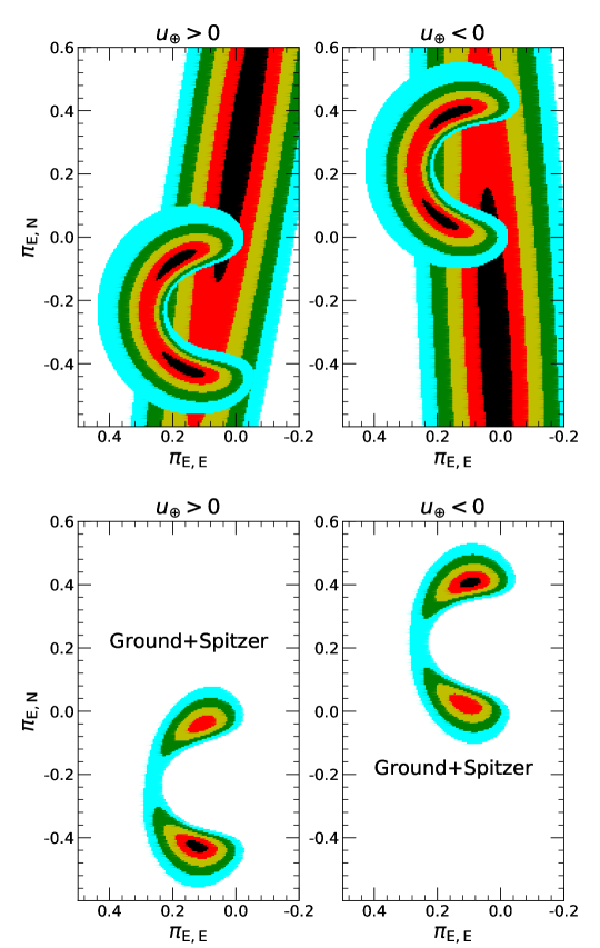
Figure 8: Parallax contours for Ground-ONLY (the elliptical contours in the top panels), Spitzer-“ONLY” (the arc-like contours in the top panels) and Ground + Spitzer (lower panels) parallax analysis. Colors (black, red, yellow, green, cyan) indicate number of $\sigma$ from the minimum (1, 2, 3, 4, 5). For both $u_{0}>0$ and $u_{0}<0$, the arc-like Spitzer-“ONLY” parallax is broken into two discrete minima due to the “1-D” constraint of ground-based parallax. The lensing parameters of the four minima are presented in Table 4.

To compare the satellite microlens parallax with the ground-based parallax, we first fit for the Spitzer-“ONLY” parallax (Jung et al., 2019a) using the method of Gould et al. (2020). We fix ($t_{0},u_{0},t_{\rm E},s,q,\alpha,\rho$) along with the $I$-band source flux as the best-fit parameters for the 2L1S ground-based parallax models and then derive a grid of ($\pi_{\rm E,N},\pi_{\rm E,E}$) with a spacing of 0.005. We repeat the analysis for both the $u_{0}>0$ and $u_{0}<0$ solutions. The resulting parallax contours are shown in the upper panels of Figure 8. The form of the Spitzer-“ONLY” contours is intermediate between the four-fold degeneracy predicted by Refsdal (1966) (and illustrated in Figure 1 of Gould 1994) and the arc-like contours analyzed by Gould (2019) for the case of late-time, monotonically declining, observations. That is, for each case ($u_{0,\oplus}>0$ and $u_{0,\oplus}<0$), there are two distinct solutions at the $1\sigma$ level, but these are connected by arcs at the $2\sigma$ level. See Gould (2019) for a discussion of these transition-contour morphologies. Figure 8 shows that the $2\sigma$ contours of the Spitzer-“ONLY” parallax overlap the $1\sigma$ contour of the ground-based parallax (and vice versa), so there is no tension between the two parallax constraints. We then fit the full-parallax models by combining the ground-based and Spitzer data. The resulting parallax contours are shown in the lower panels of Figure 8. For both $u_{0}>0$ and $u_{0}<0$, the arc-like Spitzer-“ONLY” parallax is broken into two discrete minima due to the “1-D” constraint of ground-based parallax. We label the four discrete minima in total by (“$u_{0}>0$ & small $\pi_{\rm E}$”, “$u_{0}>0$ & large $\pi_{\rm E}$”, “$u_{0}<0$ & small $\pi_{\rm E}$”, “$u_{0}<0$ & large $\pi_{\rm E}$”) and present their lensing parameters in Table 4. We find that the non-parallax parameters of the full-parallax models are consistent with the parameters of the static model at $1\sigma$.

Before making a detailed Bayesian analysis, we can roughly estimate the physical parameters and compare to the Bayesian results from the ground-based data. First, using the results of Gould (2020), we can see that the smaller-parallax local minima are strongly favored. His Equation (15) states that the relative probability of two isolated minima with equal $\chi^{2}$ from the light curve is given by

$$P\propto\rho(D_{\rm L})D_{\rm L}^{4}\pi_{\rm E}^{-1}\Phi(M)f(\bm{\mu}),$$ (A4)

where $\rho(D_{L})$ is the local density, $\Phi(M)$ is the mass function and $f(\bm{\mu})$ is the 2-D relative proper-motion distribution at $D_{\rm L}$. For the two solutions in each of the two panels of Figure 8, the parallaxes are $\pi_{\rm E}\sim 0.1$ and 0.4, the distances are $D_{\rm L}\sim 6.5$ and 4.0 kpc, and the densities are in a ratio of about 10 : 1. Hence, the combined ratios of the first three terms of Equation (A4) are $10\times(6.5/4)^{4}\times 4\sim 260$. This factor overwhelms the $\chi^{2}\sim 2$ advantage of the large-parallax solution as well as the slight differences in the last two factors. Second, combining $\pi_{\rm E}\sim 0.1$ and $\theta_{\rm E}\sim 0.37$, the lens system should have $M_{\rm L}\sim 0.45$ and $D_{\rm L}\sim 6.5$ kpc.

Finally, we repeat the Bayesian analysis for the full-parallax models and show the resulting physical parameters in Table 5. The results are quite consistent with the estimates above. In addition, Zhu et al. (2017) proposed that events should have

$$\sigma(D_{8.3})<1.4~{}{\rm kpc};\qquad D_{8.3}\equiv\frac{\rm kpc}{1/8.3+\pi_{\rm rel}/{\rm mas}}$$ (A5)

to be included in the Spitzer statistical sample. We follow the methods of Ryu et al. (2018) to fit with a PSPL model using the analogous data and conduct a Bayesian analysis without the $\theta_{\rm E}$ weight. We find $\sigma(D_{8.3})=0.7$ kpc, and thus OGLE-2019-BLG-1053Lb can be included in the statistical sample of Spitzer events if the systematics of Spitzer data does not affect the parallax measurements. However, the total flux change of the Spitzer light curve is $\sim 2.0$ instrumental flux unit, which is only a few times the level of systematics seen in other Spitzer events with observations in the baseline (Gould et al., 2020; Hirao et al., 2020; Zang et al., 2020). We therefore leave the question of whether OGLE-2019-BLG-1053Lb can be included in the final Spitzer statistical sample to a future comprehensive analysis of Spitzer planets. Here we simply note that, because the “SI” observing decision was made a week before the planetary anomaly, it was not influenced in any way by the presence of a planet, thereby satisfying a key criterion of Yee et al. (2015). Indeed, OGLE-2019-BLG-1053 is the second example (after KMT-2018-BLG-0029, Gould et al. 2020) of a very low-$q$ planetary event observed by Spitzer for which the planet remained unnoticed until well after the end of the season. This fact makes clear the need for an intensive review of all Spitzer events.

Table 1: Data used in the analysis with corresponding data reduction method and rescaling factors

Collaboration	Site	Filter	Coverage (${\rm HJD}^{\prime}$)	$N_{\rm data}$	Reduction Method	$k$	$e_{\rm min}$
OGLE		$I$	8521.9 – 8787.5	811	Wozniak (2000)	1.400	0.011
KMTNet	SSO (03)	$I$	8534.3 – 8777.9	1635	pySIS1	1.506	0.000
KMTNet	SSO (43)	$I$	8534.3 – 8777.9	1627	pySIS	1.375	0.000
KMTNet	CTIO (03)	$I$	8533.8 – 8777.5	2050	pySIS	1.207	0.000
KMTNet	CTIO (43)	$I$	8533.9 – 8775.5	2011	pySIS	1.136	0.000
KMTNet	SAAO (03)	$I$	8536.6 – 8777.3	1783	pySIS	1.335	0.000
KMTNet	SAAO (43)	$I$	8537.6 – 8777.3	1782	pySIS	1.499	0.000
Spitzer		$L$	8685.1 – 8712.0	22	Calchi Novati et al. (2015a)	2.64	0.000
KMTNet	CTIO (03)	$I$	8533.8 – 8777.5	2050	pyDIA2
KMTNet	CTIO (03)	$V$	8533.9 – 8768.5	200	pyDIA

Table 2: Parameters for PSPL and 2L1S models using Ground-based data

Parameter	PSPL	2L1S Static		2L1S Parallax
		Close	Wide	Wide $u_{0}>0$	Wide $u_{0}<0$
$\chi^{2}/dof$	12130.6/11682	11718.6/11678	11677.0/11678	11676.1/11676	11675.8/11676
$t_{0}$ (${\rm HJD}^{\prime}$)	$8690.462\pm 0.040$	$8690.538\pm 0.042$	$8690.555\pm 0.044$	$8690.572\pm 0.049$	$8690.566\pm 0.055$
$u_{0}$	$0.373\pm 0.016$	$0.355\pm 0.011$	$0.350\pm 0.010$	$0.352\pm 0.013$	$-0.350\pm 0.011$
$t_{\rm E}$	$32.8\pm 1.0$	$33.7\pm 0.7$	$34.1\pm 0.7$	$34.3\pm 1.0$	$34.4\pm 1.0$
$s$	…	$0.707\pm 0.006$	$1.406\pm 0.011$	$1.407\pm 0.013$	$1.406\pm 0.011$
$q(10^{-5})$	…	$3.14\pm 0.30$	$1.29\pm 0.10$	$1.25\pm 0.12$	$1.24\pm 0.13$
$\alpha$ (rad)	…	$0.507\pm 0.005$	$3.664\pm 0.004$	$3.683\pm 0.026$	$-3.681\pm 0.026$
$\rho(10^{-3})$	…	$2.54\pm 0.58$	$2.19\pm 0.16$	$2.08\pm 0.18$	$2.07\pm 0.22$
$\pi_{\rm E,N}$	…	…	…	$0.338\pm 0.475$	$-0.327\pm 0.515$
$\pi_{\rm E,E}$	…	…	…	$-0.012\pm 0.089$	$0.027\pm 0.053$
$I_{\rm S}$	$19.797\pm 0.064$	$19.865\pm 0.045$	$19.886\pm 0.043$	$19.877\pm 0.051$	$19.888\pm 0.044$
$I_{\rm B}$	$19.429\pm 0.044$	$19.383\pm 0.028$	$19.370\pm 0.026$	$19.377\pm 0.029$	$19.368\pm 0.026$

Table 3: Physical parameters for OGLE-2019-BLG-1053 using Ground-based data

Solutions	Physical Properties					Relative Weights
	$M_{\rm host}[M_{\odot}]$	$M_{\rm planet}[M_{\oplus}]$	$D_{\rm L}$[kpc]	$a_{\perp}$[au]	$P_{\rm bulge}$	Gal.Mod.	$\chi^{2}$
$u_{0}>0$	$0.60_{-0.24}^{+0.29}$	$2.46_{-1.00}^{+1.21}$	$6.7_{-1.0}^{+0.6}$	$3.4_{-0.5}^{+0.5}$	0.672	1.000	0.861
$u_{0}<0$	$0.62_{-0.23}^{+0.28}$	$2.50_{-0.96}^{+1.18}$	$6.8_{-0.8}^{+0.6}$	$3.4_{-0.5}^{+0.4}$	0.718	0.894	1.000
Total	$0.61_{-0.24}^{+0.29}$	$2.48_{-0.98}^{+1.19}$	$6.8_{-0.9}^{+0.6}$	$3.4_{-0.5}^{+0.5}$	0.695

Table 4: Parameters for 2L1S models using Ground-based + Spitzer data

Parameter	$u_{0}>0$ & small $\pi_{\rm E}$	$u_{0}>0$ & large $\pi_{\rm E}$	$u_{0}<0$ & small $\pi_{\rm E}$	$u_{0}<0$ & large $\pi_{\rm E}$
$\chi^{2}/dof$	11698.5/11696	11696.3/11696	11700.0/11696	11698.3/11696
$t_{0}$ (${\rm HJD}^{\prime}$)	$8690.615\pm 0.044$	$8690.586\pm 0.044$	$8690.610\pm 0.045$	$8690.603\pm 0.045$
$u_{0}$	$0.351\pm 0.009$	$0.351\pm 0.008$	$-0.350\pm 0.006$	$-0.346\pm 0.007$
$t_{\rm E}$	$34.0\pm 0.6$	$33.5\pm 0.5$	$34.1\pm 0.4$	$33.9\pm 0.5$
$s$	$1.406\pm 0.009$	$1.407\pm 0.008$	$1.404\pm 0.006$	$1.401\pm 0.007$
$q(10^{-5})$	$1.26\pm 0.09$	$1.36\pm 0.09$	$1.26\pm 0.09$	$1.31\pm 0.19$
$\alpha$ (rad)	$3.664\pm 0.004$	$3.643\pm 0.003$	$-3.664\pm 0.003$	$-3.642\pm 0.004$
$\rho(10^{-3})$	$2.11\pm 0.14$	$2.24\pm 0.16$	$2.11\pm 0.13$	$2.18\pm 0.14$
$\pi_{\rm E,N}$	$-0.027\pm 0.010$	$-0.419\pm 0.014$	$0.027\pm 0.010$	$0.416\pm 0.011$
$\pi_{\rm E,E}$	$0.114\pm 0.031$	$0.124\pm 0.031$	$0.110\pm 0.029$	$0.096\pm 0.032$
$I_{\rm S}$	$19.882\pm 0.036$	$19.881\pm 0.032$	$19.889\pm 0.023$	$19.904\pm 0.028$
$I_{\rm B}$	$19.372\pm 0.023$	$19.373\pm 0.020$	$19.368\pm 0.014$	$19.359\pm 0.017$

Table 5: Physical parameters for OGLE-2019-BLG-1053 using Ground-based + Spitzer data

Solutions	Physical Properties					Relative Weights
	$M_{\rm host}[M_{\odot}]$	$M_{\rm planet}[M_{\oplus}]$	$D_{\rm L}$[kpc]	$a_{\perp}$[au]	$P_{\rm bulge}$	Gal.Mod.	$\chi^{2}$
$u_{0}>0$	$0.49_{-0.13}^{+0.18}$	$1.99_{-0.54}^{+0.79}$	$6.6_{-0.7}^{+0.6}$	$3.3_{-0.4}^{+0.4}$	0.700	0.780	1.000
$u_{0}<0$	$0.45_{-0.13}^{+0.18}$	$1.83_{-0.56}^{+0.78}$	$6.4_{-0.8}^{+0.7}$	$3.2_{-0.5}^{+0.4}$	0.543	1.000	0.369
Total	$0.48_{-0.13}^{+0.18}$	$1.93_{-0.56}^{+0.79}$	$6.5_{-0.8}^{+0.6}$	$3.3_{-0.4}^{+0.4}$	0.650

References

- Adams et al. (2018) Adams, A. D., Boyajian, T. S., & von Braun, K. 2018, MNRAS, 473, 3608, doi: 10.1093/mnras/stx2367
- Alard & Lupton (1998) Alard, C., & Lupton, R. H. 1998, ApJ, 503, 325, doi: 10.1086/305984
- Albrow et al. (1998) Albrow, M., Beaulieu, J. P., Birch, P., et al. 1998, ApJ, 509, 687, doi: 10.1086/306513
- Albrow et al. (2009) Albrow, M. D., Horne, K., Bramich, D. M., et al. 2009, MNRAS, 397, 2099, doi: 10.1111/j.1365-2966.2009.15098.x
- Batista et al. (2011) Batista, V., Gould, A., Dieters, S., et al. 2011, A&A, 529, A102, doi: 10.1051/0004-6361/201016111
- Beaulieu et al. (2006) Beaulieu, J.-P., Bennett, D. P., Fouqué, P., et al. 2006, Nature, 439, 437, doi: 10.1038/nature04441
- Bennett et al. (2010) Bennett, D. P., Rhie, S. H., Nikolaev, S., et al. 2010, ApJ, 713, 837, doi: 10.1088/0004-637X/713/2/837
- Bennett et al. (2014) Bennett, D. P., Batista, V., Bond, I. A., et al. 2014, ApJ, 785, 155, doi: 10.1088/0004-637X/785/2/155
- Bennett et al. (2016) Bennett, D. P., Rhie, S. H., Udalski, A., et al. 2016, AJ, 152, 125, doi: 10.3847/0004-6256/152/5/125
- Bensby et al. (2013) Bensby, T., Yee, J. C., Feltzing, S., et al. 2013, A&A, 549, A147, doi: 10.1051/0004-6361/201220678
- Bensby et al. (2017) Bensby, T., Feltzing, S., Gould, A., et al. 2017, A&A, 605, A89, doi: 10.1051/0004-6361/201730560
- Bhattacharya et al. (2020) Bhattacharya, A., Bennett, D. P., Beaulieu, J. P., et al. 2020, arXiv e-prints, arXiv:2009.02329. https://arxiv.org/abs/2009.02329
- Bond et al. (2004) Bond, I. A., Udalski, A., Jaroszyński, M., et al. 2004, ApJ, 606, L155, doi: 10.1086/420928
- Bozza (2010) Bozza, V. 2010, MNRAS, 408, 2188, doi: 10.1111/j.1365-2966.2010.17265.x
- Bozza et al. (2018) Bozza, V., Bachelet, E., Bartolić, F., et al. 2018, MNRAS, 479, 5157, doi: 10.1093/mnras/sty1791
- Calchi Novati et al. (2015a) Calchi Novati, S., Gould, A., Yee, J. C., et al. 2015a, ApJ, 814, 92, doi: 10.1088/0004-637X/814/2/92
- Calchi Novati et al. (2015b) Calchi Novati, S., Gould, A., Udalski, A., et al. 2015b, ApJ, 804, 20, doi: 10.1088/0004-637X/804/1/20
- Cassan et al. (2012) Cassan, A., Kubas, D., Beaulieu, J. P., et al. 2012, Nature, 481, 167, doi: 10.1038/nature10684
- Chung et al. (2005) Chung, S.-J., Han, C., Park, B.-G., et al. 2005, ApJ, 630, 535, doi: 10.1086/432048
- Dominik (1999) Dominik, M. 1999, A&A, 349, 108
- Dominik et al. (2010) Dominik, M., Jørgensen, U. G., Rattenbury, N. J., et al. 2010, Astronomische Nachrichten, 331, 671, doi: 10.1002/asna.201011400
- Dong et al. (2009) Dong, S., Bond, I. A., Gould, A., et al. 2009, ApJ, 698, 1826, doi: 10.1088/0004-637X/698/2/1826
- Foreman-Mackey et al. (2013) Foreman-Mackey, D., Hogg, D. W., Lang, D., & Goodman, J. 2013, PASP, 125, 306, doi: 10.1086/670067
- Fukui et al. (2015) Fukui, A., Gould, A., Sumi, T., et al. 2015, ApJ, 809, 74, doi: 10.1088/0004-637X/809/1/74
- Gaia Collaboration et al. (2016) Gaia Collaboration, Prusti, T., de Bruijne, J. H. J., et al. 2016, A&A, 595, A1, doi: 10.1051/0004-6361/201629272
- Gaia Collaboration et al. (2018) Gaia Collaboration, Brown, A. G. A., Vallenari, A., et al. 2018, A&A, 616, A1, doi: 10.1051/0004-6361/201833051
- Gaudi (2012) Gaudi, B. S. 2012, ARA&A, 50, 411, doi: 10.1146/annurev-astro-081811-125518
- Gaudi et al. (2008) Gaudi, B. S., Bennett, D. P., Udalski, A., et al. 2008, Science, 319, 927, doi: 10.1126/science.1151947
- Gould (1992) Gould, A. 1992, ApJ, 392, 442, doi: 10.1086/171443
- Gould (1994) —. 1994, ApJ, 421, L75, doi: 10.1086/187191
- Gould (1996) —. 1996, ApJ, 470, 201, doi: 10.1086/177861
- Gould (2000) —. 2000, ApJ, 542, 785, doi: 10.1086/317037
- Gould (2004) —. 2004, ApJ, 606, 319, doi: 10.1086/382782
- Gould (2019) —. 2019, JKAS, 52, 121, doi: 10.5303/JKAS.2019.52.4.121
- Gould (2020) —. 2020, Journal of Korean Astronomical Society, 53, 99, doi: 10.5303/JKAS.2020.53.5.99
- Gould & Loeb (1992) Gould, A., & Loeb, A. 1992, ApJ, 396, 104, doi: 10.1086/171700
- Gould et al. (2006) Gould, A., Udalski, A., An, D., et al. 2006, ApJ, 644, L37, doi: 10.1086/505421
- Gould et al. (2010) Gould, A., Dong, S., Gaudi, B. S., et al. 2010, ApJ, 720, 1073, doi: 10.1088/0004-637X/720/2/1073
- Gould et al. (2014) Gould, A., Udalski, A., Shin, I. G., et al. 2014, Science, 345, 46, doi: 10.1126/science.1251527
- Gould et al. (2020) Gould, A., Ryu, Y.-H., Calchi Novati, S., et al. 2020, Journal of Korean Astronomical Society, 53, 9. https://arxiv.org/abs/1906.11183
- Griest & Hu (1992) Griest, K., & Hu, W. 1992, ApJ, 397, 362, doi: 10.1086/171793
- Han (2006) Han, C. 2006, ApJ, 638, 1080, doi: 10.1086/498937
- Han et al. (2017) Han, C., Udalski, A., Gould, A., et al. 2017, AJ, 154, 133, doi: 10.3847/1538-3881/aa859a
- Han et al. (2020a) Han, C., Kim, D., Jung, Y. K., et al. 2020a, AJ, 160, 17, doi: 10.3847/1538-3881/ab91ac
- Han et al. (2020b) Han, C., Udalsk, A., Gould, A., et al. 2020b, AJ, 159, 91, doi: 10.3847/1538-3881/ab6a9f
- Han et al. (2020c) Han, C., Shin, I.-G., Jung, Y. K., et al. 2020c, A&A, 641, A105, doi: 10.1051/0004-6361/202038173
- Han et al. (2021) Han, C., Udalski, A., Lee, C.-U., et al. 2021, A&A, 649, A90, doi: 10.1051/0004-6361/202039817
- Hirao et al. (2020) Hirao, Y., Bennett, D. P., Ryu, Y.-H., et al. 2020, AJ, 160, 74, doi: 10.3847/1538-3881/ab9ac3
- Hwang et al. (2018) Hwang, K.-H., Udalski, A., Shvartzvald, Y., et al. 2018, AJ, 155, 20, doi: 10.3847/1538-3881/aa992f
- Jiang et al. (2004) Jiang, G., DePoy, D. L., Gal-Yam, A., et al. 2004, ApJ, 617, 1307, doi: 10.1086/425678
- Jung et al. (2019a) Jung, Y. K., Gould, A., Udalski, A., et al. 2019a, AJ, 158, 28, doi: 10.3847/1538-3881/ab237f
- Jung et al. (2019b) Jung, Y. K., Gould, A., Zang, W., et al. 2019b, AJ, 157, 72, doi: 10.3847/1538-3881/aaf87f
- Jung et al. (2020) Jung, Y. K., Udalski, A., Zang, W., et al. 2020, AJ, 160, 255, doi: 10.3847/1538-3881/abbe93
- Kennedy & Kenyon (2008) Kennedy, G. M., & Kenyon, S. J. 2008, ApJ, 673, 502, doi: 10.1086/524130
- Kim et al. (2018a) Kim, D.-J., Kim, H.-W., Hwang, K.-H., et al. 2018a, AJ, 155, 76, doi: 10.3847/1538-3881/aaa47b
- Kim et al. (2018b) Kim, H.-W., Hwang, K.-H., Shvartzvald, Y., et al. 2018b, arXiv e-prints, arXiv:1806.07545. https://arxiv.org/abs/1806.07545
- Kim et al. (2021a) Kim, H.-W., Hwang, K.-H., Gould, A., et al. 2021a, AJ, 162, 15, doi: 10.3847/1538-3881/abfc4a
- Kim et al. (2016) Kim, S.-L., Lee, C.-U., Park, B.-G., et al. 2016, Journal of Korean Astronomical Society, 49, 37, doi: 10.5303/JKAS.2016.49.1.037
- Kim et al. (2021b) Kim, Y. H., Chung, S.-J., Yee, J. C., et al. 2021b, AJ, 162, 17, doi: 10.3847/1538-3881/abf930
- Kroupa (2001) Kroupa, P. 2001, MNRAS, 322, 231, doi: 10.1046/j.1365-8711.2001.04022.x
- Mao & Paczynski (1991) Mao, S., & Paczynski, B. 1991, ApJ, 374, L37, doi: 10.1086/186066
- Miyazaki et al. (2020) Miyazaki, S., Sumi, T., Bennett, D. P., et al. 2020, AJ, 159, 76, doi: 10.3847/1538-3881/ab64de
- Mróz et al. (2017a) Mróz, P., Han, C., Udalski, A., et al. 2017a, AJ, 153, 143, doi: 10.3847/1538-3881/aa5da2
- Mróz et al. (2017b) Mróz, P., , A., Skowron, J., et al. 2017b, Nature, 548, 183, doi: 10.1038/nature23276
- Nataf et al. (2013) Nataf, D. M., Gould, A., Fouqué, P., et al. 2013, ApJ, 769, 88, doi: 10.1088/0004-637X/769/2/88
- Nemiroff & Wickramasinghe (1994) Nemiroff, R. J., & Wickramasinghe, W. A. D. T. 1994, ApJ, 424, L21, doi: 10.1086/187265
- Paczyński (1986) Paczyński, B. 1986, ApJ, 304, 1, doi: 10.1086/164140
- Poindexter et al. (2005) Poindexter, S., Afonso, C., Bennett, D. P., et al. 2005, ApJ, 633, 914, doi: 10.1086/468182
- Refsdal (1966) Refsdal, S. 1966, MNRAS, 134, 315, doi: 10.1093/mnras/134.3.315
- Reid et al. (2014) Reid, M. J., Menten, K. M., Brunthaler, A., et al. 2014, ApJ, 783, 130, doi: 10.1088/0004-637X/783/2/130
- Ryu et al. (2018) Ryu, Y.-H., Yee, J. C., Udalski, A., et al. 2018, AJ, 155, 40, doi: 10.3847/1538-3881/aa9be4
- Schechter et al. (1993) Schechter, P. L., Mateo, M., & Saha, A. 1993, PASP, 105, 1342, doi: 10.1086/133316
- Schlafly et al. (2018) Schlafly, E. F., Green, G. M., Lang, D., et al. 2018, ApJS, 234, 39, doi: 10.3847/1538-4365/aaa3e2
- Shvartzvald et al. (2016) Shvartzvald, Y., Maoz, D., Udalski, A., et al. 2016, MNRAS, 457, 4089, doi: 10.1093/mnras/stw191
- Skowron et al. (2011) Skowron, J., Udalski, A., Gould, A., et al. 2011, ApJ, 738, 87, doi: 10.1088/0004-637X/738/1/87
- Sumi et al. (2010) Sumi, T., Bennett, D. P., Bond, I. A., et al. 2010, ApJ, 710, 1641, doi: 10.1088/0004-637X/710/2/1641
- Sumi et al. (2016) Sumi, T., Udalski, A., Bennett, D. P., et al. 2016, ApJ, 825, 112, doi: 10.3847/0004-637X/825/2/112
- Suzuki et al. (2016) Suzuki, D., Bennett, D. P., Sumi, T., et al. 2016, ApJ, 833, 145, doi: 10.3847/1538-4357/833/2/145
- Szymański et al. (2011) Szymański, M. K., Udalski, A., Soszyński, I., et al. 2011, Acta Astron., 61, 83. https://arxiv.org/abs/1107.4008
- Tomaney & Crotts (1996) Tomaney, A. B., & Crotts, A. P. S. 1996, AJ, 112, 2872, doi: 10.1086/118228
- Tsapras et al. (2009) Tsapras, Y., Street, R., Horne, K., et al. 2009, Astronomische Nachrichten, 330, 4, doi: 10.1002/asna.200811130
- Udalski (2003) Udalski, A. 2003, Acta Astron., 53, 291
- Udalski et al. (1994) Udalski, A., Szymanski, M., Kaluzny, J., et al. 1994, Acta Astron., 44, 227
- Udalski et al. (2015) Udalski, A., Szymański, M. K., & Szymański, G. 2015, Acta Astron., 65, 1. https://arxiv.org/abs/1504.05966
- Udalski et al. (2005) Udalski, A., Jaroszyński, M., Paczyński, B., et al. 2005, ApJ, 628, L109, doi: 10.1086/432795
- Witt & Mao (1994) Witt, H. J., & Mao, S. 1994, ApJ, 430, 505, doi: 10.1086/174426
- Wozniak (2000) Wozniak, P. R. 2000, Acta Astron., 50, 421
- Yee et al. (2012) Yee, J. C., Shvartzvald, Y., Gal-Yam, A., et al. 2012, ApJ, 755, 102, doi: 10.1088/0004-637X/755/2/102
- Yee et al. (2015) Yee, J. C., Gould, A., Beichman, C., et al. 2015, ApJ, 810, 155, doi: 10.1088/0004-637X/810/2/155
- Yee et al. (2021) Yee, J. C., Zang, W., Udalski, A., et al. 2021, arXiv e-prints, arXiv:2101.04696. https://arxiv.org/abs/2101.04696
- Yoo et al. (2004) Yoo, J., DePoy, D. L., Gal-Yam, A., et al. 2004, ApJ, 603, 139, doi: 10.1086/381241
- Zang et al. (2020) Zang, W., Shvartzvald, Y., Udalski, A., et al. 2020, arXiv e-prints, arXiv:2010.08732. https://arxiv.org/abs/2010.08732
- Zang et al. (2021) Zang, W., Han, C., Kondo, I., et al. 2021, arXiv e-prints, arXiv:2103.01896. https://arxiv.org/abs/2103.01896
- Zhang et al. (2020) Zhang, X., Zang, W., Udalski, A., et al. 2020, AJ, 159, 116, doi: 10.3847/1538-3881/ab6f6d
- Zhu et al. (2014) Zhu, W., Penny, M., Mao, S., Gould, A., & Gendron, R. 2014, ApJ, 788, 73, doi: 10.1088/0004-637X/788/1/73
- Zhu et al. (2017) Zhu, W., Udalski, A., Calchi Novati, S., et al. 2017, AJ, 154, 210, doi: 10.3847/1538-3881/aa8ef1