Quantum Zeno Effect in Heisenberg Picture and Critical Measurement Time

Abstract

Quantum Zeno effect is conventionally interpreted by the assumption of the wave-packet collapse, in which does not involve the duration of measurement. However, we predict duration $\tau_{m}$ of each measurement will appear in quantum Zeno effect by a dynamical approach. Moreover, there exists a model-free critical measurement time, which quantum Zeno effect does not occur when $\tau_{m}$ takes some special values. In order to give these predictions, we first present a description of quantum Zeno effect in the Heisenberg picture, which is based on the expectation value of an observable and its fluctuation. Then we present a general proof for quantum Zeno effect in the Heisenberg picture, which is independent of the concrete systems. Finally, we calculate the average population and relative fluctuation after $N$ successive measurements in XX model, which agrees with our prediction about the critical measurement time.

I Introduction

Any unstable state of a quantum system will jump to other states with the time evolution, but this transition can be inhibited by performing frequent measurements. Known as the quantum Zeno effect (QZE) Misra_1977_JMP , this phenomenon has been demonstrated to support the von Neumann’s postulate—wave-packet collapse (WPC) von_mathqm . However, many authors pointed out that the WPC is not the unique way to explain the QZE. For example, Peres suggested that a modified Hamiltonian slows down the decay of an unstable state in a two-level system Peres_1980 . It is noted that the argument for this resolution was carried out in the Schrödinger picture without using the WPC. When the QZE in atomic transition was reported by Itano et al. Itano_1990_PRA and interpreted as a witness of the WPC, Petrosky et al. understood the QZE as a dynamical process without appealing to the WPC. Their proposals could also recover Itano et al.’s experiment Petrosky_1990_PLA ; Petrosky_1991_PA . Later on, Sun et al. suggested a general dynamical approach to the QZE Sun_1995_QZE_FDP . Ai et al. studied the QZE phenomenon via the dynamical method based on "quasi-measurement"—which is substantially pre-measurement and leads to a entanglement between system and apparatus. Ai_2013 . Harrington et al. subsequently realized quasi-measurement in a superconducting qubit experiment and observed the suppression of the qubit decay Harrington_PRL_2017 .

In 2008, Bernu et al. observed suppression of photon number in a cavity quantum electrodynamics (CQED) experiment and interpreted it with the WPC Bernu_PRL_2008 . Xu et al., however, demonstrated their results could be also interpreted via the unitary evolution of a dynamical model Xu_PRA_2011 . Later, Raimond et al. also interpreted the CQED experiment by dynamical method, and further proposed to realize QZE-like phenomenon—quantum Zeno dynamics via a CQED experiment Raimond_PRL_2010 . It is found by ref.Xu_PRA_2011 that when quantum measurement process is interpreted in dynamical unitray evolution, the interaction time or measurement time $\tau_{m}$ will appear in the result, which never appears in the interpretation of the WPC. Besides, they find that there exists a critical measurement time $\tau_{m}$, where the QZE will not occur. Later, Zheng et al.’s experiment verified the critical measurement time in nuclear magnetic resonance systems Zheng_PRA_2013_QZE .

Now, whether the critical measurement time universally exists in the practical QZE still remains to be proved. This paper is ready to answer this question. To this end, we first investigate how to describe QZE only through the measurement results. From the perspective of physical observation, what we can measure is only the expectation value and fluctuation correlation of dynamical variables, which can be calculated conveniently in the Heisenberg picture. Therefore, we generally present the universal description of QZE in the Heisenberg picture. What we would like to show is that frequent measurements turn the expectation value of an observable into a constant and its fluctuation to zero. With this observation, we obtain a universal proof for QZE in the Heisenberg picture, especially a model-free critical measurement time. Without loss of generality, measurement is dynamically described by the nondemolition interaction between the system and the apparatus.

This article is organized as follows: In Sec. II, we first recall QZE phenomenon in Schrödinger picture, then reformulate it via the expectation value of an observable and its fluctuation. In Sec. III, we describe the dynamical process of QZE in the Heisenberg picture with respect to dynamical variables. In Sec. IV, we explore that under what conditions the QZE phenomenon occurs, and under these conditions, we introduce the concept of universal critical measurement time. In Sec. V, we calculate the average population and relative fluctuation after $N$ successive measurements in XX model, and discuss the numerical results. Finally, a conclusion is given in Sec. VI.

For convenience, we set $\hbar=1$ in the following discussion.

II Revisiting QZE via measurement of expectation value

Let us first recall the dynamical description of the QZE in the Schrödinger picture Xu_PRA_2011 . Suppose we have a system $S$ and an apparatus $E$, the free evolution of the system can be described by a unitary evolution operator $U(t)=\mathrm{exp}({-iHt})$, where $H=H_{0}+V$ is the Hamiltonian of $S$. $H_{0}$ and $V$ are the free Hamiltonian and the interaction that causes transitions of system states, respectively. A measurement can be given by another unitary evolution operator $M(t)=\mathrm{exp}(-iH_{\mathrm{M}}t)$, where $H_{\mathrm{M}}$ is the couplings of system $S$ to the apparatus $E$. Here, we consider the interaction Hamiltonian $H_{M}$ dominates the Hamiltonian of the total system $S$ plus $E$. Usually, we choose $[H_{0},H_{M}]=0$ which makes $M(t)$ to satisfy a quantum nondemolition (QND) measurement Braginsky_1996_RMP . Thus, by assuming $\ket{s_{i}}$ is an eigenstate of the free Hamiltonian $H_{0}$ and $\ket{e}$ is initial state of apparatus $E$, a measurement is described by a mapping

$$M(t):~{}\ket{s_{i}}\otimes\ket{e}\rightarrow\ket{s_{i}}\otimes\ket{e_{i}}~{},$$ (1)

where $\ket{e_{i}}$ is a state of $E$ corresponds to the state $\ket{s_{i}}$ of $S$. For an ideal measurement, $\ket{e_{i}}$ is orthonormal with each other, i.e., $\langle e_{i}|e_{j}\rangle=\delta_{ij}$, which leads to the measurement results could be well distinguished. Now, the QZE phenomenon with $N$ frequent measurements (see Fig.1) is described via a unitary evolution operator

$$U(\tau,\tau_{m})=\big{[}M(\tau_{m})U(\tau)\bm{]}^{N}~{},$$ (2)

where $\tau$ is a small duration of each free evolution, and $\tau_{m}$ a fixed time interval of each measurement. The relationship between $\tau$ and $N$ is $t=N\tau$, which means the total duration of the free evolution is fixed as $t$. In the large-$N$ limit, $N\rightarrow\infty$, we claim that if $U(\tau,\tau_{m})$ becomes diagonal with respect to basis $\ket{s_{i}}$, then the QZE phenomenon occurs. $U(\tau,\tau_{m})$ becomes diagonal means if the initial state of $S$ is $\ket{s_{i}}$, the final state will remain $\ket{s_{i}}$, thus this is in agreement with conventional description of the QZE with an interpretation in terms of the WPC. In the large-$N$ limit, this phenomenon will happen indeed Xu_PRA_2011 .

Figure 1: Dynamical evolution process with $N$ successive measurements. Each measurement (blue block) is followed by a free evolution (red block). Time interval of each measurement is $\tau_{m}$, and duration of each free evolution $\tau$.

However, what we can actually directly observe from the experiment is the expectation value of a system’s operator ${A}$ rather than the state of the system. Thus we need to revisit the QZE phenomenon from a perspective with respect to the expectation value. Therefore, let us firstly see a simple proposition about the expectation value: the fluctuation of an operator ${A}$ of a system is zero, if and only if the state of the system is the eigenstate of ${A}$ with egienvalue $\bar{A}$. Here, $\bar{A}$ is the expectation value of ${A}$. This is known from the identity

$$\Delta^{2}A=\langle({A}-\bar{A})\psi|({A}-\bar{A})\psi\rangle~{},$$ (3)

where $\ket{\psi}$ is the state of system. Supposing the initial states of system $S$ and apparatus $E$ are $\rho_{S}(0)$ and $\rho_{E}(0)$, respectively, we write the expectation value of ${A}$ at time $t_{N}=(\tau+\tau_{m})N$ as

$$\bar{A}(t_{N})=\mathrm{Tr}\big{(}{A}U(\tau,\tau_{m})\rho_{S}(0)\otimes\rho_{E}(0)U(\tau,\tau_{m})^{\dagger}\big{)}~{}.$$ (4)

Thus, by this proposition we claim that if

$$\bar{A}(t_{N})\rightarrow\bar{A}(0),~{}~{}~{}\Delta^{2}A(t_{N})\rightarrow 0$$ (5)

in the large-$N$ limit, then the state of the system will be $\rho_{S}(0)$. Here, $\bar{A}(0)$ is the initial expectation value of ${A}$ given by $\mathrm{Tr}\big{(}{A}\rho_{S}(0)\otimes\rho_{E}(0)\big{)}$, and we assume $H_{M}$ is not degenerate. With this observation, we use Eq.(5) instead of disappearance of $U(\tau,\tau_{m})$’s off-diagonal parts in the large-$N$ limit to describe the QZE phenomenon.

III QZE in the Heisenberg picture

We have reformulated QZE phenomenon via the expectation value: The expectation value of an observable and its fluctuation turn into a constant and zero respectively, due to frequent measurements. It is convenient to calculate the expectation value of an observable in the Heisenberg picture. Thus we now choose the Heisenberg picture to investigate QZE phenomenon.

Suppose the initial Hamiltonian of the system $S$ and the initial interaction Hamiltonian between $S$ and apparatus $E$ are $H=H_{0}+V$ and $H_{M}$ respectively. Here, $V$ causes transitions among the states of the system $S$, which satisfies $[H_{0},V]\neq 0$. We choose $[H_{0},{H_{M}}]=0$ to satisfy the QND measurement condition Braginsky_1996_RMP . If we wish to measure a dynamical variable ${A}$, $A$ should satisfy conditions $[H_{0},A]=0$ and $[{H_{M}},A]=0$. Then, we describe the dynamical process of $N$ successive measurements (see Fig.1) for variable $A$ in the Heisenberg picture as

$$i{\dot{A}}(t)=[{A}(t),V(t)]$$ (6)

when $t_{k}\leq t<t_{k}+\tau$, and

$$i{\dot{A}}(t)=0$$ (7)

when $t_{k}+\tau\leq t<t_{k+1}$. Eq.(7) means $A$ does not evolute with $H_{M}$ when measurements are carried out. We have denoted $t_{k}$ by $(\tau+\tau_{m})k$, and $k$ is an integer that satisfies $0<k\leq N$. The total duration of free evolution is still fixed as $t=N\tau$. In order to form closed equations, we write down the Heisenberg equations of motion about other variables as follows:

$$\left\{\begin{split}i{\dot{V}}(t)&=[{V}(t),H(t)]=[{V}(t),H_{0}(t)]~{},\\ i{\dot{H}_{0}}(t)&=[{H_{0}}(t),H(t)]=[H_{0}(t),{V}(t)]~{},\\ i{\dot{H}_{M}}(t)&=[{H_{M}}(t),H(t)]=[{H_{M}}(t),V(t)]~{},\end{split}\right.$$ (8)

when $t_{k}\leq t<t_{k}+\tau$, and

$$\left\{\begin{split}i{\dot{V}}(t)&=[V(t),H_{M}(t)]~{},\\ i\dot{H}_{0}(t)&=0~{},\\ i{\dot{H}_{M}}(t)&=0~{},\end{split}\right.$$ (9)

when $t_{k}+\tau\leq t<t_{k+1}$. In the above arguments, there is an implied assumption that the interaction Hamiltonian dominates the total Hamiltonian when measurements are carried out.

Next, we can claim that if the initial state of the system is an eigenstate of $H_{0}$, and the solution $A(t_{N})$ corresponding to Eq.(6) and Eq.(7) satisfies

$$A(t_{N})\rightarrow A(t_{0})$$ (10)

in the large-$N$ limit, then the QZE phenomenon occurs. This is obvious if one notes that observable $A^{2}(t_{N})$ will also tend to $A^{2}(t_{0})$. Thus, the expectation value and fluctuation will turn into a constant and zero, respectively. In the next section, we will show that Eq.(10) indeed is satisfied due to frequent measurement. From Eq.(10), we see that $[V,{H_{M}}]\neq 0$ must be satisfied, otherwise, the frequent measurements can not affect the evolution of operator $A$ and no QZE phenomenon can occur. Thus, we assume $[V,{H_{M}}]\neq 0$ in the following discussion.

IV Universal critical measurement time

We next answer the question what can make the Eq.(10) satisfy. The recursion relation of $A(t_{k})$ reads as

$$A(t_{k})=-i\int_{t_{k-1}}^{t_{k-1}+\tau}[A(s),V(s)]\mathrm{d}s+A(t_{k-1})$$ (11)

in accordance with the Eq.(6) and Eq.(7). It follows from the recursion relation that

$$A(t_{N})=-i\sum_{k=1}^{N}\int_{t_{k-1}}^{t_{k-1}+\tau}[A(s),V(s)]\mathrm{d}s+A(t_{0})~{}.$$ (12)

Thus, for a short $\tau$ or a large $N$ with fixed $t$, $A(t_{N})$ is approximated as

$$A(t_{N})\simeq-i\tau\sum_{k=1}^{N}[A,V](t_{k-1})+A(t_{0})~{}.$$ (13)

For convenience, we denote $[A,V](t)$ by $X(t)$, and its Heisenberg equations of motion is described from Eqs.(8) and Eqs.(9) as

$$\left\{\begin{split}i\dot{X}(t)&=[X(t),H(t)]~{},~{}~{}t_{k}\leq t<t_{k}+\tau~{},\\ i\dot{X}(t)&=[X(t),H_{M}(t)]~{},~{}~{}t_{k}+\tau\leq t<t_{k+1}~{}.\end{split}\right.$$ (14)

Similarly, the recursion relation of $X(t_{k})$ via Eq.(14) gives

$$\begin{split}X(t_{k})&=-i\sum_{l=0}^{k-1}\int_{t_{l}+\tau}^{t_{l+1}}[X(s),H_{M}(s)]\mathrm{d}s-\\ &~{}~{}~{}~{}i\sum_{l=0}^{k-1}\int_{t_{l}}^{t_{l}+\tau}[X(s),H(s)]\mathrm{d}s+X(t_{0})~{}.\end{split}$$ (15)

Denoting $X(t_{k})$ to the zero-order with respect to $\tau$ by $X(k\tau_{m})$, we obtain

$$X(k\tau_{m})=-i\int_{0}^{k\tau_{m}}[X(s),{H_{M}(s)]}\mathrm{d}s+X(t_{0})~{}.$$ (16)

On the base vectors of $H_{0}$, ${H_{M}}$ and $X$ are expressed as

$$\left\{\begin{split}{H_{M}}(t_{0})&=\sum_{n}{H(n)}|s_{n}\rangle\langle s_{n}|~{},\\ X(t_{0})&=\sum_{mn}x_{nm}|s_{n}\rangle\langle s_{m}|~{},\end{split}\right.$$ (17)

where $\ket{s_{n}}$ is a common eigenstate of $A$, $H_{0}$ and $H_{M}$. $H(n)$ is a Hermitian operator on the Hilbert space $\mathcal{H}_{E}$ of apparatus $E$. The spectral decomposition of $H(n)$ is given by

$$H(n)=\sum_{\alpha}h_{\alpha}(n)|\sigma_{\alpha}(n)\rangle\langle\sigma_{\alpha}(n)|~{},$$ (18)

where $|\sigma_{\alpha}(n)\rangle$ is eigenstate of $H(n)$ with eigenvalue $h_{\alpha}(n)$.

Because of $X=[A,V]$, one can find $x_{nn}=0$. Thus, solving the integral equation(16) with the initial condition(17), we obtain

$$X(k\tau_{m})=\sum_{n\neq l}x_{nl}e^{iH(n)k\tau_{m}}e^{-iH(l)k\tau_{m}}|s_{n}\rangle\langle s_{l}|~{}.$$ (19)

Finally, substituting Eq.(19) into Eq.(13), we obtain $A(t_{N})$ as (for more details see Appendix A)

$$\begin{split}A(t_{N})&=-i\tau\sum_{n\neq l,\alpha,\beta}\frac{\sin[(h_{\alpha}(l)-h_{\beta}(n))N\tau_{m}/2]}{\sin[(h_{\alpha}(l)-h_{\beta}(n))\tau_{m}/2]}\times\\ &~{}~{}~{}~{}x_{nl}y_{\beta\alpha}(nl){e^{-i(h_{\alpha}(l)-h_{\beta}(n))(N-1)\tau_{m}/2}\times}\\ &~{}~{}~{}~{}|s_{n},\sigma_{\beta}(n)\rangle\langle s_{l},\sigma_{\alpha}(l)|+A(t_{0})+o(\tau)~{},\end{split}$$ (20)

where $y_{\beta\alpha}(nl)=\langle\sigma_{\beta}(n)|\sigma_{\alpha}(l)\rangle$.

From the above expression of $A(t_{N})$, one can see that when

$${\sin[\big{(}h_{\alpha}(l)-h_{\beta}(n)\big{)}\frac{\tau_{m}}{2}\bigg{]}\neq 0~{},}$$ (21)

$A(t_{N})$ will tend to $A(t_{0})$ as $N$ tends to infinity. In order to satisfy this condition, we additionally require: i) $H_{M}$ is not degenerate, namely, $h_{\alpha}(l)\neq h_{\beta}(n)$ and ii)

$$\tau_{m}\neq\frac{2k\pi}{h_{\alpha}(l)-h_{\beta}(n)}~{},$$ (22)

where $k$ is an integer and $n\neq l$. Thus, when these two requirements are both satisfied, the QZE phenomenon will occur according to the arguments in the last section. Set

$$\tau_{m}^{*}=\frac{2k\pi}{h_{\alpha}(l)-h_{\beta}(n)}~{}.$$ (23)

Hence, when $\tau_{m}=\tau_{m}^{*}$ but $\Lambda_{S}$ is not degenerate, $A(t_{N})$ can not still tend to $A(t_{0})$ as $\tau$ tends to zero. Thus, $\tau_{m}^{*}$ is a critical measurement time, which QZE phenomenon can not occur when the value of $\tau_{m}$ equals $\tau_{m}^{*}$. Since our approach does not depend on a concrete physical model, it is concluded that the critical measurement time $\tau_{m}^{*}$ quite universally exists in the QZE phenomenon. One can note that the magnitude of $\tau_{m}^{*}$ only depends on the energy spectral structure of the couplings of the system $S$ to the apparatus $E$, due to the assumption of QND measurement.

The effect of critical measurement time was firstly demonstrated by Xu et al., where they calculated the average photon number after $N$ successive measurements for a cavity-QED model and found the photon number could not be suppressed when $\tau_{m}$ took some special values Xu_PRA_2011 . Later, the critical measurement time of a spin model was calculated by Zheng et al., and they verified it via a nuclear magnetic resonance experiment Zheng_PRA_2013_QZE . Thus, the critical measurement time was calculated model by model previously. Now, we obtain a model-free expression of the critical measurement time, and prove it can universally exist in the practical QZE. Moreover, since the WPC does not involve the duration $\tau_{m}$ of measurement, the effect of critical measurement time can not be explained in terms of the WPC. Thus, the effect of critical measurement time is a significant prediction of the dynamical approach, which largely differs from the prediction of the WPC.

It is pointed out that the expression of critical measurement time $\tau_{m}^{*}$ must be also obtained in the Schrödinger picture, due to the equivalence of the two pictures. Thus, we give a complete derivation for $\tau_{m}^{*}$ in the Schrödinger picture in Appendix B.

V XX model

Consider a chain of $L$ two-level systems with the Hamiltonian

$$H=\sum_{n=0}^{L-1}\frac{1}{2}\omega\sigma_{n}^{z}+g(\sigma_{n}^{+}\sigma_{n+1}^{-}+\sigma_{n}^{-}\sigma_{n+1}^{+})~{}.$$ (24)

Here, $\sigma_{n}^{+}=(\sigma_{n}^{-})^{\dagger}=|e\rangle_{n}\langle\mathrm{g}|$, $\sigma_{n}^{z}=|e\rangle_{n}\langle e|-|\mathrm{g}\rangle_{n}\langle\mathrm{g}|$; $|e\rangle_{n}$ and $|\mathrm{g}\rangle_{n}$ are excited and ground states respectively in the $n$-th site of this chain. This is the XX model Sachdev_QPT_2011 , and could be exactly solvable.

We wish to measure the excited population of site-0. Then the Hamiltonian for measurement reads as

$$H_{M}=\sigma_{0}^{+}\sigma_{0}^{-}\otimes\Sigma_{E}~{},$$ (25)

where $\Sigma_{E}$ is an operator on the Hilbert space of apparatus $E$.

To consider time evolution of the chain, we use the Jordan-Wigner transform,

$$\sigma_{n}^{z}=2c_{n}^{\dagger}c_{n}-1~{},~{}~{}~{}\sigma_{n}^{+}=c_{n}^{\dagger}\prod_{i=0}^{n-1}(-\sigma_{i}^{z})~{},$$ (26)

to get a free spinless fermion Hamiltonian,

$$H=\sum_{n=0}^{L-1}\omega c^{\dagger}_{n}c_{n}+g(c_{n}^{\dagger}c_{n+1}+c_{n+1}^{\dagger}c_{n})~{}.$$ (27)

Meanwhile, the initial Hamiltonian for measurement is transformed into

$$H_{M}=c_{0}^{\dagger}c_{0}\otimes\Sigma_{E}~{}.$$ (28)

Applying the Fourier transform $c_{n}=\frac{1}{\sqrt{L}}\sum_{k=0}^{L-1}$$e^{i\frac{2\pi}{L}nk}b_{k}$, we write down the simple diagonal form from Eq.(27)

$$H=\sum_{k=0}^{L-1}\varepsilon_{k}b^{\dagger}_{k}b_{k}~{},$$ (29)

where $\varepsilon_{k}=\omega+2g\cos(2\pi k/L)$. Thus, we obtain the time evolution of the element of single particle reduced density matrix

$$\begin{split}\langle c^{\dagger}_{n}c_{m}\rangle(t)&=\sum_{k,q=0}^{L-1}\frac{1}{L}e^{i\frac{2\pi}{L}mq-i\frac{2\pi}{L}nk}e^{i(\varepsilon_{k}-\varepsilon_{q})t}\langle b_{k}^{\dagger}b_{q}\rangle(0)\\ &=\sum_{x,y=0}^{L-1}f(n,m,x,y,t)\langle c^{\dagger}_{x}c_{y}\rangle(0)~{},\end{split}$$ (30)

which is also the lattice correlation function. Here,

$$\begin{split}f(n,m,x,y,t)&=\sum_{k,q=0}^{L-1}\frac{1}{L^{2}}e^{i\frac{2\pi}{L}(m-y)q-i\frac{2\pi}{L}(n-x)k}\times\\ &~{}~{}~{}~{}e^{i(\varepsilon_{k}-\varepsilon_{q})t}~{}.\end{split}$$ (31)

Similarly, the dynamics of measurement evolution is also written as

$$\langle c_{n}^{\dagger}c_{m}\rangle(t)=\langle c_{n}^{\dagger}c_{m}\rangle(0)g(n,m,t)~{},$$ (32)

where

$$g(n,m,t)=\left\{\begin{split}&e^{i\Sigma_{E}t},~{}~{}~{}n=0,m\neq 0\\ &e^{-i\Sigma_{E}t},~{}~{}~{}m=0,n\neq 0\\ &1,~{}~{}~{}\mathrm{others}\end{split}\right.~{}.$$ (33)

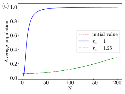
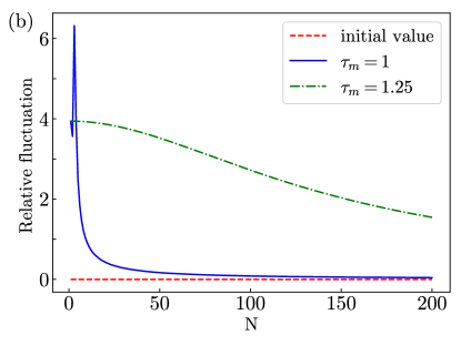
Figure 2: Average population (a) and its relative fluctuation (b) as a function of measurement number $N$. We fix $t=N\tau=1$, and choose $r_{E}=g=5$, $L=30$. The average population and relative fluctuation rapidly tend to a constant and zero (red dashed line), respectively, when $\tau_{m}=1$ (blue solid line). But, this doesn’t occur when $\tau_{m}$ is chosen specifically at $1.25$ (green dash-dotted line), which is close to a critical measurement time.

According to Eq.(30) and Eq.(32), the recursion relation of $\langle c_{n}^{\dagger}c_{m}\rangle(t_{k})$ and $\langle c_{n}^{\dagger}c_{m}\rangle(t_{k-1})$ is expressed as

$$\begin{split}\langle{c}_{n}^{\dagger}{c}_{m}\rangle(t_{k})&=\langle{c}_{n}^{\dagger}{c}_{m}\rangle(t_{k-1}+\tau)g(n,m,\tau_{m})\\ &=\sum_{x,y=0}^{L-1}F(n,m,x,y,\tau,\tau_{m})\langle{c}_{x}^{\dagger}{c}_{y}\rangle(t_{k-1})~{},\end{split}$$ (34)

where $F(n,m,x,y,\tau,\tau_{m})=f(n,m,x,y,\tau)g(n,m,\tau_{m})$. We arrange $\langle{c}_{n}^{\dagger}{c}_{m}\rangle(t_{k})$ into a column vector in order of $00,01,\cdots,0L-1,10,\cdots,L-1L-1$, and denote this vector by $C(t_{k})$. Similarly, we arrange $F(n,m,x,y,\tau,\tau_{m})$ into a matrix in the same order, and denote it by $F(\tau,\tau_{m})$. Thus, we rewrite Eq.(34) as

$$C(t_{k})=F(\tau,\tau_{m})C(t_{k-1})~{}.$$ (35)

According to Eq.(35), we obtain the relation between $C(t_{N})$ and $C(t_{0})$,

$$C(t_{N})=F(\tau,\tau_{m})^{N}C(t_{0})~{}.$$ (36)

Assuming that the initial condition of the chain is $\langle{c}_{0}^{\dagger}{c}_{0}\rangle(t_{0})=1$, and $\langle{c}_{m}^{\dagger}{c}_{n}\rangle(t_{0})=0$ for other $m,n$, which means that the initial state of site-0 is in excited state, and remaining sites are in ground state. The initial state of apparatus part is the eigenstate of $\Sigma_{E}$ with eigenvalue $r_{E}$. Under this initial condition, we write

$$\langle{c}_{0}^{\dagger}{c}_{0}\rangle(t_{N})=F(\tau,\tau_{m})^{N}(00,00)~{},$$ (37)

where $F(\tau,\tau_{m})^{N}(00,00)$ is denoted by the first row and the first column element of matrix $F(\tau,\tau_{m})^{N}$. Because of $(c_{0}^{\dagger}c_{0})^{2}=c_{0}^{\dagger}c_{0}$, the relative fluctuation is expressed as

$$\frac{\Delta\langle{c}_{0}^{\dagger}{c}_{0}\rangle(t_{N})}{\langle{c}_{0}^{\dagger}{c}_{0}\rangle(t_{N})}=\sqrt{\frac{1}{\langle{c}_{0}^{\dagger}{c}_{0}\rangle(t_{N})}-1}~{}.$$ (38)

In this case, it is difficulty to give a specific analytic expression of $F(\tau,\tau_{m})^{N}(00,00)$, so the critical measurement time can not be directly obtained from $F(\tau,\tau_{m})^{N}(00,00)$. However, according to the expression of critical measurement time, we directly write

$$\tau_{m}^{*}=\frac{2k\pi}{r_{E}}~{},$$ (39)

where $k$ is an integer. Thus, when $\tau_{m}\neq 2k\pi/r_{E}$ and $\tau$ tends to zero, $\langle{c}_{0}^{\dagger}{c}_{0}\rangle(t_{N})$ will tend to $\langle{c}_{0}^{\dagger}{c}_{0}\rangle(t_{0})$, and $\Delta\langle{c}_{0}^{\dagger}{c}_{0}\rangle(t_{N})/\langle{c}_{0}^{\dagger}{c}_{0}\rangle(t_{N})$ will tend to zero.

The numerical results of average population and its relative fluctuation on site-0 are shown in Fig.2 and Fig.2. In our calculation, $t=N\tau=1$, $r_{E}=g=5$, $L=30$ are used. For measurement time $\tau_{m}$, we choose two values $1$ (blue line) and $1.25$ (green line), which the later is close to the critical time $2\pi/r_{E}$. When $\tau_{m}=1$, average population and relative fluctuation rapidly tend one and zero, respectively. Thus, we know QZE phenomenon occurs. However, when $\tau_{m}$ is chosen at $1.25$, average population does not rapidly tend to one, so does not relative fluctuation. These numerical results are in agreement with our prediction about the universal effect of critical measurement time.

VI Conclusion

In conclusion, the QZE phenomenon has been revisited in Heisenberg picture. Here, when the expectation value of an observable and its fluctuation turn into a constant and zero respectively in the large-$N$ limit, we judge that the QZE phenomenon happens. With this observation, we present a universal proof for QZE in Heisenberg picture. Moreover, by studying the QZE in Heisenberg picture, we predict that it is universal that there exists critical measurement time $\tau_{m}^{*}$ and give a general expression for it. The expression of $\tau_{m}^{*}$ does not depend on a concrete physical model, but the magnitude of $\tau_{m}^{*}$ depends on the energy spectral structure of the couplings of the system $S$ to the apparatus $E$, due to the assumption of QND measurement. This is a generalization of previous results, since the critical measurement time is only discussed in some concrete examples before. We also derive the expression of $\tau_{m}^{*}$ in Schrödinger picture, due to the equivalence of the two pictures. It is pointed out that the prediction about critical measurement time can not be explained by the WPC, due to the disappearance of the interaction duration $\tau_{m}$ in the WPC. Thus, the existence of critical measurement time is the key criterion to distinguish experimentally which is correct between the WPC and the dynamic method. Our numerical results in XX model are in agreement with the prediction about the universal critical measurement time.

Appendix A The expression of $A(t_{N})$

Because of Eq.(13) and the discussion in the Sec. IV, $A(t_{N})$ is given by

$$A(t_{N})=-i\tau\sum_{k=0}^{N-1}X(k\tau_{m})+A(t_{0})+o(\tau)~{}.$$ (40)

According to Eq.(18) and Eq.(19), $X(k\tau_{m})$ is rewritten by

$$\begin{split}X(k\tau_{m})&=\sum_{n\neq l,\alpha,\beta}x_{nl}y_{\beta\alpha}(nl)e^{-i(h_{\alpha}(l)-h_{\beta}(n))k\tau_{m}}\times\\ &~{}~{}~{}~{}|s_{n},\sigma_{\beta}(n)\rangle\langle s_{l},\sigma_{\alpha}(l)|~{},\end{split}$$ (41)

where $y_{\beta\alpha}(nl)=\langle\sigma_{\beta}(n)|\sigma_{\alpha}(l)\rangle$.

Substituting Eq.(41) into Eq.(40), we obtain

$$\begin{split}A(t_{N})&=-i\tau\sum_{k=0}^{N-1}\sum_{n\neq l,\alpha,\beta}x_{nl}y_{\beta\alpha}(nl)e^{-i(h_{\alpha}(l)-h_{\beta}(n))k\tau_{m}}\times\\ &~{}~{}~{}~{}|s_{n},\sigma_{\beta}(n)\rangle\langle s_{l},\sigma_{\alpha}(l)|+A(t_{0})+o(\tau)\\ &=-i\tau\sum_{n\neq l,\alpha,\beta}\frac{\sin[(h_{\alpha}(l)-h_{\beta}(n))N\tau_{m}/2]}{\sin[(h_{\alpha}(l)-h_{\beta}(n))\tau_{m}/2]}\times\\ &~{}~{}~{}~{}x_{nl}y_{\beta\alpha}(nl){e^{-i(h_{\alpha}(l)-h_{\beta}(n))(N-1)\tau_{m}/2}\times}\\ &~{}~{}~{}~{}|s_{n},\sigma_{\beta}(n)\rangle\langle s_{l},\sigma_{\alpha}(l)|+A(t_{0})+o(\tau)~{}.\end{split}$$ (42)

Therefore, we obtain the expression of $A(t_{N})$.

Appendix B Critical measurement time in Schrödinger picture

We can also derive critical measurement time in the Schrödinger picture. $U(\tau)$ is defined as the unitary evolution operator of system $S$ with the "measurement" turned off, and $M(\tau_{m})$ is the unitary measurement operator, we have

$$U(\tau)=\mathrm{e}^{-\mathrm{i}\tau H},\quad M(\tau_{m})=\mathrm{e}^{-\mathrm{i}\tau_{m}H_{M}}$$ (43)

and $U(\tau,\tau_{m})$ is evolution operator of the whole process with $N$ frequent repeated measurements

$$U(\tau,\tau_{m})=\quantity[M(\tau_{m})U(\tau)]^{N}~{}.$$ (44)

We rewrite $U(\tau,\tau_{m})$ by $U_{k}(\tau)\equiv M(\tau_{m})^{k}U(\tau)M(\tau_{m})^{-k}$ as an multiproduct

$$U(\tau,\tau_{m})=\quantity[\prod_{k=1}^{N}U_{k}(\tau)]M(\tau_{m})^{N}~{}.$$ (45)

For short $\tau$ or large $N$, we expand $U_{k}(\tau)$ to the first order of $\tau$

$$\begin{split}U_{k}(\tau)&\approx 1-\mathrm{i}\tau M(\tau_{m})^{k}HM(\tau_{m})^{-k}\equiv 1-\mathrm{i}\tau H_{k}~{},\end{split}$$ (46)

where $H_{k}=M(\tau_{m})^{k}HM(\tau_{m})^{-k}$. The explicit form of $H_{k}$’s matrix elements is given as

$$H_{k}=H_{d}+\sum_{m\neq n}H_{mn}\mathrm{e}^{-\mathrm{i}k\tau_{m}H(m)}\mathrm{e}^{\mathrm{i}k\tau_{m}H(n)}\outerproduct{s_{m}}{s_{n}}~{},$$ (47)

where $H_{d}$ is the diagonal term of $H$. Substituting Eq.(46), Eq.(47) and Eq.(17) into Eq.(45), we obtain

$$U(\tau,\tau_{m})\approx\quantity(1-\mathrm{i}tH_{d}-\mathrm{i}\frac{t}{N}\Gamma)M(\tau_{m})^{N}~{},$$ (48)

where

$$\begin{split}\Gamma&=\sum_{k}\sum_{m\neq n}H_{mn}\mathrm{e}^{-\mathrm{i}k\tau_{m}H(m)}\mathrm{e}^{\mathrm{i}k\tau_{m}H(n)}\outerproduct{s_{m}}{s_{n}}\\ &=\sum_{m\neq n}\Lambda_{mn}H_{mn}\outerproduct{s_{m}}{s_{n}}~{},\\ \Lambda_{mn}&=\sum_{k=1}^{N}\mathrm{e}^{-\mathrm{i}k\tau_{m}H(m)}\mathrm{e}^{\mathrm{i}k\tau_{m}H(n)}~{}.\end{split}$$ (49)

Taking Eq.(18) into account, we obtain

$$\mathrm{e}^{-\mathrm{i}k\tau_{m}H(m)}=\sum_{\alpha}\mathrm{e}^{-\mathrm{i}k\tau_{m}h_{\alpha}(m)}\outerproduct{\sigma_{\alpha}(m)}{\sigma_{\alpha}(m)}~{}.$$ (50)

Thus

$$\begin{split}\Lambda_{mn}&=\sum_{k=1}^{N}\sum_{\alpha\beta}y_{\alpha\beta}(mn)\mathrm{e}^{-\mathrm{i}k\tau_{m}h_{\alpha}(m)}\mathrm{e}^{\mathrm{i}k\tau_{m}h_{\beta}(n)}\times\\ &~{}~{}~{}~{}\outerproduct{\sigma_{\alpha}(m)}{\sigma_{\beta}(n)}\\ &=\sum_{\alpha\beta}y_{\alpha\beta}(mn)\quantity[\sum_{k=1}^{N}\mathrm{e}^{-\mathrm{i}k\tau_{m}(h_{\alpha}(m)-h_{\beta}(n))}]\times\\ &~{}~{}~{}~{}\outerproduct{\sigma_{\alpha}(m)}{\sigma_{\beta}(n)}~{},\end{split}$$ (51)

where $y_{\alpha\beta}=\innerproduct{\sigma_{\alpha}(m)}{\sigma_{\beta}(n)}$. If $\mathrm{e}^{-\mathrm{i}\tau_{m}(h_{\alpha}(m)-h_{\beta}(n))}\neq 1$ the summation over $k$ is

$$\begin{split}\sum_{k=1}^{N}\mathrm{e}^{-\mathrm{i}k\tau_{m}(h_{\alpha}(m)-h_{\beta}(n))}&=\frac{\sin[\frac{1}{2}\tau_{m}N(h_{\alpha}(m)-h_{\beta}(n))]}{\sin[\frac{1}{2}\tau_{m}(h_{\alpha}(m)-h_{\beta}(n))]}\times\\ &~{}~{}~{}~{}\mathrm{e}^{-\mathrm{i}\tau_{m}(N+1)(h_{\alpha}(m)-h_{\beta}(n))/2}~{}.\end{split}$$ (52)

The above equation tells us that $\Lambda_{mn}$ is finite when $\mathrm{e}^{-\mathrm{i}\tau_{m}(h_{\alpha}(m)-h_{\beta}(n))}\neq 1$ . Thus, we have

$$\lim_{N\rightarrow\infty}\frac{\Gamma}{N}=0~{}.$$ (53)

This means the vanishing of off-diagonal terms of unitary evolution operator due to the frequent measurement, or there is QZE in other words. However, when

$$\tau_{m}=\frac{2l\pi}{h_{\alpha}(m)-h_{\beta}(n)}\equiv\tau_{m}^{*}$$ (54)

which means $\mathrm{e}^{-\mathrm{i}\tau_{m}(h_{\alpha}(m)-h_{\beta}(n))}=1$, Eq.(53) not hold anymore, the off-diagonal terms of evolution operator remains when $N\rightarrow\infty$, the QZE can not occur, making $\tau_{m}^{*}$ the critical measurement time.

References

- [1] B. Misra and E. C. G. Sudarshan. The zeno’s paradox in quantum theory. Journal of Mathematical Physics, 18(4):756–763, 1977.
- [2] John Von Neumann. Mathematical Foundations of Quantum Mechanics. Princeton University Press, Princeton, 1955.
- [3] Asher Peres. Zeno paradox in quantum theory. American Journal of Physics, 48(11):931–932, 1980.
- [4] Wayne M. Itano, D. J. Heinzen, J. J. Bollinger, and D. J. Wineland. Quantum zeno effect. Phys. Rev. A, 41:2295–2300, Mar 1990.
- [5] T. Petrosky, S. Tasaki, and I. Prigogine. Quantum zeno effect. Physics Letters A, 151(3):109 – 113, 1990.
- [6] T. Petrosky, S. Tasaki, and I. Prigogine. Quantum zeno effect. Physica A: Statistical Mechanics and its Applications, 170(2):306 – 325, 1991.
- [7] C. P. Sun, Xue-Xi Yi, and Xia-Ji Liu. Quantum dynamical approach of wavefunction collapse in measurement process and its application to quantum zeno effect. Fortschritte der Physik/Progress of Physics, 43(7):585–612, 1995.
- [8] Qing Ai, Dazhi Xu, Su Yi, A. G. Kofman, C. P. Sun, and Franco Nori. Quantum anti-zeno effect without wave function reduction. Scientific Reports, 3(1):1752, May 2013.
- [9] P. M. Harrington, J. T. Monroe, and K. W. Murch. Quantum zeno effects from measurement controlled qubit-bath interactions. Phys. Rev. Lett., 118:240401, Jun 2017.
- [10] J. Bernu, S. Deléglise, C. Sayrin, S. Kuhr, I. Dotsenko, M. Brune, J. M. Raimond, and S. Haroche. Freezing coherent field growth in a cavity by the quantum zeno effect. Phys. Rev. Lett., 101:180402, Oct 2008.
- [11] D. Z. Xu, Qing Ai, and C. P. Sun. Dispersive-coupling-based quantum zeno effect in a cavity-qed system. Phys. Rev. A, 83:022107, Feb 2011. arXiv:1007.4634.
- [12] J. M. Raimond, C. Sayrin, S. Gleyzes, I. Dotsenko, M. Brune, S. Haroche, P. Facchi, and S. Pascazio. Phase space tweezers for tailoring cavity fields by quantum zeno dynamics. Phys. Rev. Lett., 105:213601, Nov 2010. arXiv:1007.4942.
- [13] Wenqiang Zheng, D. Z. Xu, Xinhua Peng, Xianyi Zhou, Jiangfeng Du, and C. P. Sun. Experimental demonstration of the quantum zeno effect in nmr with entanglement-based measurements. Phys. Rev. A, 87:032112, Mar 2013.
- [14] V. B. Braginsky and F. Ya. Khalili. Quantum nondemolition measurements: the route from toys to tools. Rev. Mod. Phys., 68:1–11, Jan 1996.
- [15] S. Sachdev. Quantum phase transitions, . Cambridge University Press, Cambridge ; New York, 2011.