Källén–Lehmann Spectral Representation of the Scalar SU(2) Glueball

Abstract

The estimation of the Källén-Lehmann spectral density from gauge invariant lattice QCD two point correlation functions is proposed, and explored via an appropriate inversion method. As proof of concept the SU(2) glueball spectrum for the quantum numbers $J^{PC}=0^{++}$ is investigated for various values of the lattice spacing. The spectral density and the glueball spectrum are estimated using the published data of [1]. Our estimates for the ground state mass are in good agreement with the traditional approach published therein, which is based on the large time exponential behaviour of the correlation functions. Furthermore, the spectral density also contains hints of excites states in the spectrum.

1 Introduction

A major effort to understand the dynamics of strong interactions is the computation of the hadronic spectra. In QCD, hadrons, namely mesons and baryons, are seen as bound states of quarks and gluons. Besides the conventional hadronic states, multiple-quark and pure glue bound states are also predicted by theory. Of these exotic states, so far only multi-quark states have been identified experimentally [2]. For glueballs there are a number of candidate states [3, 4, 5], but no established observation. Glueballs continue to attract a great deal of theoretical [6, 7, 8, 9, 10, 11, 12] and experimental attention, with an ongoing effort to identify these pure glue states unambiguously [13, 14, 15, 16]. Additionally, glueball states have also been discussed as possible candidates for dark matter [1, 17].

A first principles approach to access the hadron spectra, which has been advancing since the beginning of the eighties from last century [18], is lattice QCD. In a typical lattice QCD computation of the bound state mass, an appropriate two point correlation function is evaluated and, from its large time decay behaviour and the associated slope, the ground state mass is estimated [19]. In the discrete setting, it is in general tricky to access a priori continuum quantities from finite volume data, [20], although ways to extract more than naively expected from finite volume input have been devised [21]. It is common practise in the computation of bound masses to rely on techniques that improve the signal to noise ratio of the Monte Carlo simulation. These techniques allow access not only to the ground state mass with the chosen quantum numbers, but, sometimes, also allow the first excited state to be extracted. In practice however, the computation of the excited states masses has proven to be a difficult task, usually based on a generalized eigenvalue problem, as in [4, 5].

Herein, we aim to discuss an alternative way of accessing the particle masses: via the computation of the Källén-Lehmann spectral representation associated with the momentum space particle propagator [22]. A possible advantage of using spectral representations compared to a conventional lattice calculation is that it does not necessarily require the use of smearing, or other techniques, to improve the Monte Carlo signal to noise ratio, see e.g. [23, 24] and references therein. As seen below, the computation of the spectral function allows simultaneous extraction of the ground state and, to some extent, also of the 1st excited state, at least for good enough data.

The interest in the Källén-Lehmann spectral representation goes beyond the determination of particle spectra. Besides accessing the spectra at zero and finite temperature, the spectral representation is linked with the analytical structure of the associated propagator [25], and it allows the computation of thermodynamical and transport properties [26]. Furthermore, in QCD, or any other confining theory, it can help to understand the confinement mechanism [27, 28, 29, 30, 31, 32, 33]. In particular for the glueball sector, future work should focus on the thermal widening of the spectral peaks, indicative of a melting pattern of the glueball modes across (or at least near to) the deconfinement transition. Such information cannot be directly traced from the aforementioned large time slope and requires a more in depth study of the spectral functions themselves [8]. A first step set in this paper is developing an efficient inversion scheme at zero temperature that can be quite easily generalized to finite temperature afterwards.

In the current work we focus on the SU(2) glueball states with quantum numbers $J^{PC}=0^{++}$, i.e. the scalar glueball. However, in principle, the procedure can be extended to other quantum numbers and other gauge groups. As discussed below, the masses of the glueball $0^{++}$ obtained from the spectral function are in good agreement with the estimates of a more conventional mass calculation.

Let us describe our procedure to access the Källén-Lehmann spectral representation $\rho(\omega)$ from a two point correlation function $G(p^{2})$. The relation between these two functions reads

$$G(p^{2})=\int_{0}^{\infty}\frac{2\omega\rho(\omega)\differential{\omega}}{\omega^{2}+p^{2}}=\int_{-\infty}^{\infty}\frac{\rho(\omega)\differential{\omega}}{\omega-ip}\ .$$

This definition assumes that the integrations are well defined [34] and, therefore, $\rho(\omega)$ approaches zero sufficiently fast as $|\omega|\rightarrow\infty$. Certain correlators contain polynomial terms that diverge for large $p$ as happens e.g. for the glueball operator, something which follows immediately from power counting and a dimensional analysis. However in these cases it is still possible to write down a sensible Källén–Lehmann spectral representation, if one first subtracts the polynomial part [34]. This corresponds to adding appropriate contact counterterms. So, if $G(p^{2})$ has a polynomial part, the propagator can be written as

$$G(p^{2}) =\sum_{k=0}^{n-1}a_{k}(p^{2}-\bar{p}^{2})^{k}+(-p^{2}+\bar{p}^{2})^{n}\int_{0}^{\infty}\frac{2\omega\tilde{\rho}(\omega)\differential{\omega}}{\omega^{2}+p^{2}}$$ (1)

$$=\sum_{k=0}^{n-1}a_{k}(p^{2}-\bar{p}^{2})^{k}+(-p^{2}+\bar{p}^{2})^{n}\int_{-\infty}^{\infty}\frac{\tilde{\rho}(\omega)\differential{\omega}}{\omega-ip}$$

with

$$a_{k} =\frac{1}{k!}\partialderivative[k]{G(p^{2})}{(p^{2})}\Bigg{|}_{p^{2}=\bar{p}^{2}},$$ (2)

$$\tilde{\rho}(\omega) =\frac{\rho(\omega)}{(\omega^{2}+\bar{p}^{2})^{n}},$$ (3)

and $\bar{p}^{2}$ is a reference momentum scale at which the subtraction is done. A derivation of the above relations can be found in appendix A. For the scalar glueball a dimensional analysis [10] shows that $n=3$. The spectral function $\rho(\omega)$ can thus be obtained, if the subtraction of the polynomial part can be performed. However, performing subtractions on numerical data is extremely sensitive to the choice of $\bar{p}$ and results in relative rapid variation of $\{a_{k}\}$ with the subtraction point [35].

An elegant way to perform the subtractions, without actually having to do these, is by considering the Fourier transform of $G(p^{2})$ and look at the Schwinger function defined as

$$C(\tau)=\mathcal{F}\left\{G(p^{2})\right\}(\tau)=\int_{-\infty}^{\infty}G(p^{2})\bigg{|}_{\vec{p}=0,p_{4}\neq 0}~{}e^{-ip_{4}\tau}\differential{p_{4}}.$$ (4)

Setting the subtraction reference momentum $\bar{p}=0$, yields

$$C(\tau) =\mathcal{F}\left\{G(p^{2})\right\}(\tau)$$ (5)

$$=\mathcal{L}\left\{\rho(\omega)\right\}(|\tau|)+2\pi\sum_{k=0}^{n-1}a_{k}(-1)^{k}\delta^{(2k)}(\tau)$$ (6)

$$\quad+4\pi(-1)^{n+1}\sum_{k=2}^{n}\delta^{(2(n-k)+2)}(\tau)\int_{0}^{\infty}\differential{\omega}\omega^{2k-3}\tilde{\rho}(\omega)\,,$$

see appendix A for more details. The important observation however, is that $C(\tau)=\mathcal{L}\left\{\rho(\omega)\right\}(|\tau|)$ when $\tau~{}\neq~{}0$, and equal to a sum of (derivatives of) Dirac delta functions when $\tau=0$. Therefore, $\rho(\omega)$ can be recovered by taking $C(\tau)$ for $\tau>0$, and inverting the Laplace transformation.

Because the inverse Laplace transform is an ill-defined numerical problem, regularization is necessary in order to perform the inversion. We shall use Tikhonov regularization, similar to our previously published method [28, 36]. However, because glueballs are observable particles, their spectral density $\rho(\omega)$ is non-negative. Therefore we shall implement Tikhonov regularization using Non-Negative Least Squares (NNLS) [37], to ensure a positive spectral function $\rho(\omega)\geq 0$. Tikhonov regularization is not the only possible way to regularize the inversion, and a number of different regularization strategies have been explored in literature to access the spectral function for particle correlators by various authors [38, 39, 40, 41, 42, 43, 33, 31, 44, 45]. An advantage of the Tikhonov regularization being that it keeps the optimization function a quadratic function, which translates into solving a modified linear system of equations. Using a NNLS solver allows solving this system of linear equations while simultaneously enforcing positivity; a feature not shared by other strategies to enforce positivity such as the ansatz $\rho(\omega)=\exp\pqty{\sigma(\omega)}$. The most widely used approach is based on the maximum entropy method (MEM) [38]. We will therefore use the same litmus test as in [38] to benchmark our approach, before turning to the actual glueball case.

2 The Numerical Method

In a lattice simulation the propagator $G(p_{n})$ is computed on a finite set of evenly spaced momenta $p_{n}$. Given a data set $\{G(p_{n})\}:=\{G(p_{0}),\ldots,G(p_{N-1})\}$, the Schwinger function is computed using DFFT, resulting in a data set $\{C(\tau_{k})\}$, where

$$C(\tau_{k})=\sum_{n=0}^{N-1}G(p_{n})e^{-i2\pi kn/N}.$$

The Laplace transformation to access the spectral function is given by

$$C(\tau_{k})=\mathcal{L}\left\{\rho(\omega)\right\}(\tau_{k})=\int_{0}^{\infty}e^{-\omega\tau_{k}}\rho(\omega)\differential{\omega}.$$ (7)

Because $\rho(\omega)\geq 0$ for observable particles, $\partialderivative*{C}{\tau}\leq 0$. Equation 7 can be approximated using the matrix equation

$$\boldsymbol{C}=\boldsymbol{K}\boldsymbol{\rho},$$

with the elements of $\boldsymbol{K}$ defined as

$$\boldsymbol{K}_{k\ell}:=e^{-\omega_{\ell}\tau_{k}}\Delta\omega.$$

Since $\boldsymbol{\rho}$ needs to be obtained, and a direct solution is impossible due to the near zero singular values of $\mathbf{K}$, the original problem is replaced by the minimisation of the Tikhonov regularizing functional

$$J_{\alpha}=\norm{\boldsymbol{K}\boldsymbol{\rho}-\boldsymbol{C}}_{2}^{2}+\alpha^{2}\norm{\boldsymbol{\rho}-\boldsymbol{\rho}^{*}}_{2}^{2},$$ (8)

where $\alpha^{2}>0$ is the Tikhonov parameter and $\boldsymbol{\rho}^{*}$ is a prior estimate for $\boldsymbol{\rho}$. In order to impose the constraint $\boldsymbol{\rho}\geq 0$ using a NNLS solver, we define

$$\boldsymbol{A}=\matrixquantity(\boldsymbol{K}\\ \alpha\mathbb{1}),\quad\boldsymbol{b}=\matrixquantity(\boldsymbol{C}\\ \alpha\boldsymbol{\rho}^{*}),$$ (9)

and rewrite $J_{\alpha}$ as

$$J_{\alpha}=\norm{\boldsymbol{A}\boldsymbol{\rho}-\boldsymbol{b}}_{2}^{2}.$$ (10)

It is straightforward to show that (8) and (10) are equivalent. However, the formulation of the problem using Eq. (10) can be solved with a non-negative least squares (NNLS) solver such that $\boldsymbol{\rho}\geq 0$ is guaranteed [37]. In this work we used the implementation of NNLS [37] as provided by SciPy [46].

We should note that although we work with lattice QCD data, we nevertheless keep using the “continuum version” of the spectral relation, as also done in e.g. [38, 43, 31]. The standard MEM paper [38, Appendix], compared the usage of an (artificial) lattice kernel against the continuum kernel, and did not find any noticeable difference. This provides justification for this assumption.

Determination of $\alpha$

The regularization parameter $\alpha$, in essence, provides a soft threshold to the singular values of $\boldsymbol{K}$, such that the smallest singular values no longer cause numerical issues. Choosing $\alpha$ is a delicate affair, since setting it too small means the problem remains ill-defined, whereas setting it too large destroys a lot of the information contained in the data.

Our preferred criterion for $\alpha^{2}$ relies on the Morozov discrepancy principle [36], which states that $\alpha^{2}$ should be chosen such that

$$\norm{\boldsymbol{K}\boldsymbol{\rho}-\boldsymbol{C}}_{2}^{2}=\sum_{i}\sigma_{i}^{2},$$ (11)

where $\sum_{i}\sigma_{i}^{2}$ is the total variance in the data. Intuitively, this criterion implies that the quality of the reconstruction is identical to the quality of the data. The $\alpha^{2}$ obeying eq. 11 is guaranteed to be unique [47], and because the value of $\boldsymbol{\rho}$ for a given data set $\boldsymbol{C}$ depends only on $\alpha^{2}$, any minimization algorithm yields the same solution for $\boldsymbol{\rho}$. We found fast convergence with Nelder-Mead, as implemented in symfit [48], but we checked that different solvers indeed give numerically the same solution.

Construction of $\boldsymbol{K}$

The matrix $\boldsymbol{K}$ should perform the Laplace transform as truthfully as possible, and therefore $\omega$ should range from $[0,\omega_{\text{max}})$, where $\omega_{\text{max}}$ is sufficiently large compared to any features that might appear in $\rho(\omega)$. In order to ensure this we choose to sample $\omega$ evenly in logarithmic space from $[10^{-5},10^{5}]$ $\text{\,}\mathrm{GeV}$ in $N_{\omega}$ steps. However, the peak positions are very consistent, in both linear and logarithmic space, provided $\omega_{\text{max}}$ and $N_{\omega}$ are large enough. Nonetheless, sampling $\omega$ evenly in logarithmic space is preferred, as convergence of the peak positions is reached for much smaller values of $N_{\omega}$. A numerical comparison is provided in appendix B.

3 Results and Discussion

In this section we detail the results of applying the method of section 2 to various mock and real data. In section 3.1 the method is applied to a toy model based on a vector-meson spectral density to establish its reliability. Then, in section 3.2 the method is applied to recent lattice SU(2) propagator data for the $0^{++}$ glueball [1].

3.1 Meson toy-model

Figure 1: Reconstruction the toy-model spectral density function for various noise levels $d$ as defined in eq. 14 and number of data points $N$. The dashed black line is the original spectral function, while the blue solid curve is the reconstructed spectral function as given by the Tikhonov regularized NNLS method.

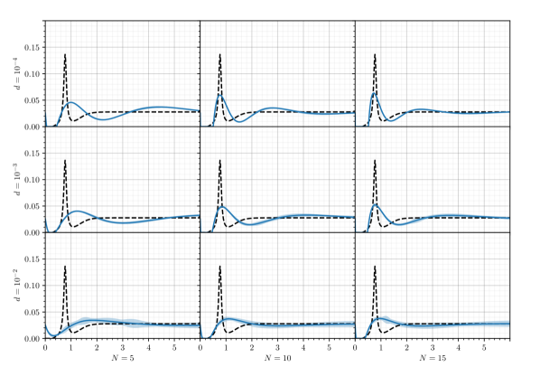
In order to investigate the reliability of the method we consider a realistic toy-model, based on a vector-meson model decay into hadrons, as used before in [38]. This particular model needs a single subtraction ($n=1$), and therefore provides an excellent test of the method. To allow comparison of our results to those of [38], the same process was used to generate the mock data. The meson spectral density function is given by

$$\rho(\omega)=\frac{2}{\pi}\bqty{F^{2}_{\rho}\frac{\Gamma_{\rho}m_{\rho}}{(\omega^{2}-m_{\rho}^{2})^{2}+\Gamma_{\rho}^{2}m_{\rho}^{2}}+\frac{1}{8\pi}\pqty{1+\frac{\alpha_{s}}{\pi}}\frac{1}{1+e^{(\omega_{0}-\omega)/\delta}}},$$ (12)

with an energy-dependent width

$$\Gamma_{\rho}(\omega)=\frac{g_{\rho\pi\pi}^{2}}{48\pi}m_{\rho}\pqty{1-\frac{4m_{\pi}^{2}}{\omega^{2}}}^{3/2}\theta\pqty{\omega-2m_{\pi}}.$$ (13)

The empirical values of the parameters are

$$m_{\rho} =0.77\text{ GeV},\quad m_{\pi}=0.14\text{ GeV},$$

$$g_{\rho\pi\pi} =5.45, F_{\rho}=\frac{m_{\rho}}{g_{\rho\pi\pi}},$$

$$\omega_{0} =1.3\text{ GeV}, \delta=0.2\text{ GeV}.$$

As $\omega\to\infty$, this model behaves like $\rho(\omega\to\infty)=(1/4\pi^{2})(1+\alpha_{s}/\pi)$. Therefore the integral section 1 does not converge, and a single subtraction has to be performed; that means $n=1$ in the notation used in eq. 2.

Assuming $\alpha_{s}=0.3$, the value $(1/4\pi^{2})(1+\alpha_{s}/\pi)=0.0277$ can be used as the prior, but identical to [38] we shall use the slightly smaller value $\rho_{\text{prior}}~{}=~{}0.0257$. In order to generate mock data, we compute $C_{\text{orig}}(\tau_{k})$ as the Laplace transform of $\rho(\omega)$, on $N$ points $\tau_{k}$ spaced by $\Delta\tau=0.085\text{ fm}=0.43078\text{ GeV}^{-1}$. The standard deviation of the noise is chosen as

$$\sigma(\tau_{k})=d\,C_{\text{orig}}(\tau_{k})\frac{\tau_{k}}{\Delta\tau},$$ (14)

where $d$ is a parameter which controls the noise level, identical to that of [38]. The mock data set is then generated as

$$C(\tau_{k})=\mathcal{N}(\mu=C_{\text{orig}}(\tau_{k}),\sigma^{2}=\sigma\pqty{\tau_{k}}^{2}).$$

These mock data sets were then inverted, ignoring $C(\tau_{0})$, for various values of $N$ and $d$, using the method of section 2, to test the robustness of the method. No inversions without positivity constraints were performed, as significant positivity violations were observed in initial trials. Here we used $N_{\omega}=1000$ in the construction of $\boldsymbol{K}$. The results are shown in fig. 1. Both more data-points, or less noise, are found to improve the quality of the reconstruction. A direct comparison with [38, Figure 4] is complicated by the absence of uncertainties on that figure, but the performance of the methods seems comparable to the naked eye.

3.2 SU(2) Glueball data

Yamanaka et al. [1], see also [49], have provided us with the Schwinger functions for the SU(2) pure Yang-Mills glueballs, using lattice simulations for $\beta=$ 2.1, 2.2, 2.3, 2.4, 2.5. The Schwinger functions were computed using the raw data, that is, without any smearing applied. The lattice volumes, the number of configurations, the number of Schwinger function time slices $N$, and the uncertainties in each data set, are shown in table 1. There was no access possible to the configuration per configuration data, implying we have to ignore any possible correlations between the different times. Said otherwise, we work with a diagonal correlation matrix.

The simulations of Yamanaka et al. rely on large ensembles of configurations, resulting in data sets with very low statistical uncertainties. This makes the results of the Tikhonov regularized inversion highly reproducible, as seen in the toy model study of section 3.1. For further details about the data sets, we refer the reader to [1].

$\beta$	Volume	Volume ($\text{\,}\mathrm{f}\mathrm{m}^{4}$)	Configurations	$N$	$\max(C(\tau))/\expectationvalue{\sigma_{C}(\tau)}$	$a\sqrt{\sigma}$
$2.1$	$10^{3}\times 12$	$(2.73)^{3}\times 3.27=66.30$	1,000,000	7	$3.28\times 10^{-4}$	$0.608(16)$
$2.2$	$12^{4}$	$(2.51)^{3}\times 2.51=39.87$	9,999,990	7	$1.04\times 10^{-4}$	$0.467(10)$
$2.3$	$14^{3}\times 16$	$(2.31)^{3}\times 2.65=32.80$	4,100,000	9	$1.38\times 10^{-4}$	$0.3687(22)$
$2.4$	$16^{3}\times 24$	$(1.91)^{3}\times 2.86=19.90$	2,030,000	13	$1.55\times 10^{-4}$	$0.2660(21)$
$2.5$	$20^{3}\times 24$	$(1.69)^{3}\times 2.02=\,\;9.72$	520,000	13	$3.04\times 10^{-4}$	$0.1881(28)$

Table 1: The glueball data sets of [1]. Selection of information taken from [1, Table I, Table II]. The physical volume in units of $\text{\,}\mathrm{f}\mathrm{m}^{4}$ was calculated assuming $\sqrt{\sigma}=0.44$ $\text{\,}\mathrm{GeV}$.

figure[.45][][b] figure[.45][][b]

Figure 2: $C(\tau)$ for all data sets. In order to display negative values while keeping log-scale where possible, the range $[-10^{-7},10^{-7}]$ is linear. Only the data points connected by a dotted line were included in the inversion.

Figure 3: $\rho(\omega)$ for all data sets, using the $ip$-method. The $\rho(\omega)$ have been normalized to give the last peak an intensity of 1. The colored bands indicate the masses as found by [1] (see also table 2). The oscillations indicate overfitting and clearly positivity constraints should be imposed.

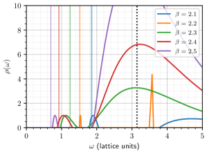
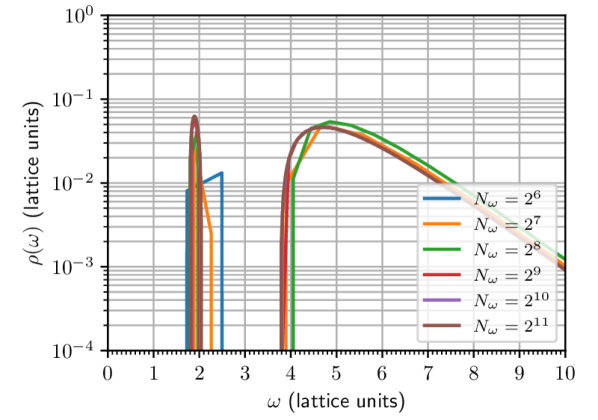
The Schwinger functions for the various simulations can be seen in fig. 3. The values of $C(\tau)$ for $\tau>10$ behave unexpectedly, since $\rho(\omega)\geq 0$ implies $\partialderivative*{C}{\tau}~{}\leq~{}0$. Therefore these data points were excluded from the inversion, as this behavior is likely the result of lattice artifacts. On the basis of this argument perhaps even more data points could be excluded, but we found that this does not significantly impact the result, and given the small number of data points available and in the interest of transparency, we have opted to include as many data points as possible in the inversion. Figure 3 shows the spectral density functions as obtained without any constraints on $\rho(\omega)$, using the $ip$-method published in [36]. As fig. 3 illustrates, there are significant positivity violations and rapid oscillations in the infrared when positivity is not enforced, especially for small $\omega$, a tell-tale sign of overfitting. On the other hand, when positivity is imposed, the resulting spectral functions in fig. 5 all display a clear mass gap that corresponds to a ground state mass in the range of $1.4\text{\,}\mathrm{GeV}$ to $1.9\text{\,}\mathrm{GeV}$. Moreover, the infrared oscillations are gone, and we can actually forget about the deep IR that is anyhow inaccessible to the lattice simulation. To produce fig. 5, we set $N_{\omega}=2000$ in the construction of $\boldsymbol{K}$. This is unnecessarily large for reliable extraction of the ground state mass, as convergence is already reached for $N_{\omega}\geq 1000$ as is shown in appendix B, and was done merely to improve the aesthetics of fig. 5. Figure 5 lists the $\omega$ values of all the local maxima in fig. 5, and the left and right Half Width at Half Maximum (HWHM) values of each local maximum.

In order to compare the ground state masses as extracted via the spectral method with the results calculated by Yamanaka et al. [1], table 2 lists the two results side by side.

figure[][][c] table[][][c] $\beta$ $\omega\pm\text{HWHM}$ (lattice units) 2.1 $1.895+0.112-0.085$ $4.708+1.499-0.747$ 2.2 $1.540+0.018-0.035$ $3.571+0.041-0.041$ 2.3 $1.116+0.195-0.110$ $3.110+1.653-0.909$ 2.4 $1.053+0.170-0.136$ $3.219+1.654-0.914$ 2.5 $0.808+0.068-0.054$ $3.039+1.615-0.838$

Figure 4: $\rho(\omega)$ for all data sets, subject to $\rho(\omega)~{}\geq~{}0$, normalized such that the ground state has an intensity of $1$. The colored bands indicate the masses as found by [1] (see also table 2). The dotted line at $\omega=\pi$ (lattice units) indicates the largest momentum at which the results can be trusted.

Figure 5: Maxima of fig. 5 in order of increasing $\omega$, with corresponding left and right Half Width at Half Maximum (HWHM).

	Traditional [1]		Spectral representation
$\beta$	$am_{\phi}$	$m_{\phi}$ /GeV	$am_{\phi}$	$m_{\phi}$ /GeV
2.1	1.853(13)	1.341(37)	1.895(99)	1.371(80)
2.2	1.517(10)	1.429(32)	1.540(26)	1.451(40)
2.3	1.241(6)	1.481(11)	1.116(153)	1.331(182)
2.4	0.924(8)	1.528(18)	1.053(153)	1.742(254)
2.5	0.696(6)	1.628(28)	0.808(61)	1.890(145)

Table 2: The $0^{++}$ glueball ground state masses as presented in Table 3 of [1] compared with the spectral representation method. The uncertainty in the ground state mass values was calculated by fitting a Gaussian distribution to the entire ground state peak. The physical units were calculated assuming $\sqrt{\sigma}=0.44$ $\text{\,}\mathrm{GeV}$.

The uncertainties in the ground state masses as listed in table 2 were calculated by fitting a Gaussian distribution to the ground state peak, and a string tension of $\sqrt{\sigma}=$0.44\text{\,}\mathrm{GeV}$$ was assumed to convert to physical units. The required values of $a\sqrt{\sigma}$ are given in table 1, and their uncertainties were compounded with the uncertainties in the ground state mass to calculate the uncertainties in the physical mass $m_{\phi}$.

For all but $\beta=2.5$, the scalar glueball masses as obtained by [1], and those extracted using the spectral density method, agree within one standard deviation. This is noteworthy, since we based ourselves on unsmeared data, whilst the mass estimates from [1] were obtained after smearing, which usually improves the ground state signal. For $\beta=2.5$ the disagreement is about $\sim 1.8$ standard deviations, which might be explained by the fact that this is also the data set generated from the smallest number of configurations. In addition to the ground states, the spectra presented in fig. 5 also hint at first excited states. However, the position of these excited states are close to or beyond $\pi/a$, the largest momentum accessible on the lattice, and thus their estimation has to be treated with care.

Figure 6 displays the extracted mass estimates as a function of $a^{2}$, from which an estimate for the continuum values of the masses can be obtained after performing a weighted linear regression to the function $m_{\phi}(a^{2})=sa^{2}+m_{\phi}(0)$. This model is motivated by the fact that the lattice action and operators have corrections of $\order{a^{2}}$. The continuum estimates for the ground and excited state masses were found to be $m_{\phi}(0)=1.68\pm 0.09$ $\text{\,}\mathrm{GeV}$ and $m_{\phi}(0)=4.07\pm 1.01$ $\text{\,}\mathrm{GeV}$ respectively (where again we assumed $\sqrt{\sigma}=0.44$ $\text{\,}\mathrm{GeV}$).

Figure 6: Mass estimates of the ground and excites states, see fig. 5, vs $a^{2}$ in $\text{\,}\mathrm{f}\mathrm{m}^{2}$. A weighted linear regression to the data points was performed to estimate the continuum values for the ground and excited state masses.

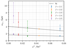
The relatively wide peaks for the excited states indicate that we might need a better signal, as there are in principle no decay channels open for these 1st excited states in pure gluodynamics, not even to the $0^{++}$ ground state. However, these values are near to or beyond $\omega=\pi/a$, i.e. the resolution of the lattice experiments, and hence are to be taken with a grain of salt. Only the $\beta=2.2$ data set displays relatively sharp ground and excited state peaks; we dare to speculate that this is because of the much larger configuration number for $\beta=2.2$ (table 1). Future research should reveal whether larger configuration numbers and/or smearing techniques result in sharper peaks. It is nonetheless reassuring that this crude estimate for the continuum 1st excited state mass comes pretty close to the state of the art prediction of [50, Table 23], based on independent SU(2) data.

We should also keep in mind that we are aiming at reliable continuum estimates, which implies $\beta$ and the lattice volume should be sufficiently large, so probably values of $\beta\geq 2.4$ are suboptimal from this viewpoint. The size of the (inverse) lattice spacing also determines the maximally accessible momentum scale, forcing our spectral function estimates to vanish in the UV, in contradistinction with the continuum tail going as $\omega^{4}$, as follows from power counting or explicit computation [51].

4 Summary and Conclusion

In this work we discuss the computation of the Källén-Lehmann spectral density function $\rho$ from two point correlation functions $G(p^{2})$ that can have a (divergent) polynomial part. The extraction of the finite part of $G(p^{2})$ that is associated with $\rho$ requires the subtraction of that polynomial part. To avoid doing the subtraction directly on the numerical data, an operation that can be cumbersome and a source of large uncertainties, we consider the Schwinger function $C(\tau)$ instead of $G(p^{2})$. Once the Schwinger function has been calculated from $G(p^{2})$, subtractions are performed simply by removing the data point $C(0)$. The spectral density is then obtained by taking the inverse Laplace transform of $C(\tau)$ for $\tau>0$. For this inverse Laplace transform, the inversion method as described in [36], that does not constrain $\rho$, was compared with a reformulation of the method that relies on a non-negative least square solver to impose a positive $\rho$.

The numerical method was first tested on mock data from a given spectral density. The test followed the same rules as used in the original maximum entropy method inversion paper [38], with similar results.

The inversion method was then applied to extract the Källén-Lehmann spectral density function from the lattice SU(2) glueball propagator data with quantum numbers $J^{PC}=0^{++}$, based on the unsmeared data of [1]. We found that the inversion method is robust and allows estimation of the ground state and provides hints of excited state masses. The comparison of the mass estimates between a conventional lattice approach [1] and the method described herein shows that the latter achieves comparable results for the ground state, despite the lack of smearing.

The new spectral method is sufficiently general to be applied to any spectroscopic calculation. In future research, we will scrutinize the usage of smeared data to boost the contribution of the lowest lying states, which should allow access to at least the 1st excited state with higher accuracy. Afterwards, the analysis performed in the current manuscript might also be extended to the analysis of the spectra of other glueball states with different quantum numbers.

5 Acknowledgements

The authors are indebted to N. Yamanaka, H. Iida, A. Nakamura and M. Wakayama for sharing the Schwinger function estimates based on their data of [1]. We also thank A. Athenodorou and M. Teper for useful communication.

O.O. was partly supported by the FCT – Fundação para a Ciência e a Tecnologia, I.P., under project numbers UIDB/04564/2020 and UIDP/04564/2020, while the work of D.D. and M.R. was supported by KU Leuven IF project C14/16/067.

Appendix A Subtracted correlator

A correlator $G(p^{2})$ can be expressed in terms of a Källén–Lehmann spectral representation as

$$G(p^{2})=\int_{0}^{\infty}\frac{2\omega\rho(\omega)\differential{\omega}}{\omega^{2}+p^{2}},$$ (15)

if this integral converges. However, if the correlator contains divergences polynomial in $p^{2}$, it is still possible to find a Källén–Lehmann spectral representation, if one first subtracts the polynomial part. In order to do this, consider the Taylor expansion of $G(p^{2})$ around $\bar{p}$:

$$G(p^{2})=\sum_{k=0}^{n-1}(p^{2}-\bar{p}^{2})^{k}\partialderivative[k]{G(p^{2})}{(p^{2})}\Bigg{|}_{p^{2}=\bar{p}^{2}}+\tilde{G}_{n}(p^{2}).$$ (16)

where $\tilde{G}_{n}(p^{2})$ is the remainder after the first $n$ terms have been isolated. At zeroth order, we find

$$\tilde{G}_{1}(p^{2}) =G(p^{2})-G(\bar{p}^{2})$$

$$=(-p^{2}+\bar{p}^{2})\int_{0}^{\infty}\frac{2\omega\rho(\omega)\differential{\omega}}{(\omega^{2}+\bar{p}^{2})(\omega^{2}+p^{2})}$$ (17)

Through induction, we obtain

$$\tilde{G}_{n}(p^{2})=(-p^{2}+\bar{p}^{2})^{n}\int_{0}^{\infty}\frac{2\omega\rho(\omega)\differential{\omega}}{(\omega^{2}+\bar{p}^{2})^{n}(\omega^{2}+p^{2})}$$ (18)

This allows us to state that

$$G(p^{2}) =\sum_{k=0}^{n-1}a_{k}(p^{2}-\bar{p}^{2})^{k}+(-p^{2}+\bar{p}^{2})^{n}\int_{0}^{\infty}\frac{2\omega\tilde{\rho}(\omega)\differential{\omega}}{\omega^{2}+p^{2}}$$

$$=\sum_{k=0}^{n-1}a_{k}(p^{2}-\bar{p}^{2})^{k}+(-p^{2}+\bar{p}^{2})^{n}\int_{-\infty}^{\infty}\frac{\tilde{\rho}(\omega)\differential{\omega}}{\omega-ip}$$ (19)

with

$$a_{n} =\frac{1}{n!}\partialderivative[n]{G(p^{2})}{(p^{2})}\Bigg{|}_{p^{2}=\bar{p}^{2}},$$ (20)

$$\tilde{\rho}(\omega) =\frac{\rho(\omega)}{(\omega^{2}+\bar{p}^{2})^{n}}.$$ (21)

Because $\rho$ is an odd (real) function for bosonic degrees of freedom [38], so is $\tilde{\rho}$. We will now calculate the Fourier transform of the subtracted correlator, in order to obtain $C(\tau)$.

$$\mathcal{F}\left\{G(p^{2})\right\} =\underbrace{\sum_{k=0}^{n-1}a_{k}\mathcal{F}\left\{(p^{2})^{k}\right\}}_{A}+\underbrace{\mathcal{F}\left\{(-p^{2})^{n}\int_{-\infty}^{\infty}\frac{\tilde{\rho}(\omega)\differential{\omega}}{\omega-ip}\right\}}_{B}$$ (22)

where we have set $\bar{p}=0$. For the first term $A$ we obtain

$$A=\sum_{k=0}^{n-1}a_{k}\mathcal{F}\left\{(p^{2})^{k}\right\} =2\pi\sum_{k=0}^{n-1}a_{k}(-1)^{k}\delta^{(2k)}(\tau)$$ (23)

and for the second

$$B =\mathcal{F}\left\{(-p^{2})^{n}\int_{-\infty}^{\infty}\frac{\tilde{\rho}(\omega)\differential{\omega}}{\omega-ip}\right\}$$ (24)

$$=\int_{0}^{\infty}\differential{\omega}\tilde{\rho}(\omega)\mathcal{F}\left\{\frac{2\omega(-p^{2})^{n}}{\omega^{2}+p^{2}}\right\}$$ (25)

$$=2\pi(-1)^{n}\int_{0}^{\infty}\differential{\omega}\tilde{\rho}(\omega)\left[-2\sum_{k=2}^{n}\omega^{2k-3}\delta^{(2(n-k)+2)}(\tau)+\omega^{2n}e^{-|\tau|\omega}\right]$$

$$=4\pi(-1)^{n+1}\sum_{k=2}^{n}\delta^{(2(n-k)+2)}(\tau)\int_{0}^{\infty}\differential{\omega}\omega^{2k-3}\tilde{\rho}(\omega)+\mathcal{L}\left\{\tilde{\rho}(\omega)\omega^{2n}\right\}(|\tau|)$$

As a result the total transform is given by

$$\mathcal{F}\left\{G(p^{2})\right\} =2\pi\sum_{k=0}^{n-1}a_{k}(-1)^{k}\delta^{(2k)}(\tau)+\mathcal{L}\left\{\rho(\omega)\right\}(|\tau|)$$ (26)

$$\quad+4\pi(-1)^{n+1}\sum_{k=2}^{n}\delta^{(2(n-k)+2)}(\tau)\int_{0}^{\infty}\differential{\omega}\omega^{2k-3}\tilde{\rho}(\omega)$$

An important consequence of this is that all the subtractions are turned into (derivatives of) delta functions, which end up at $\tau=0$. Therefore, taking only $\tau>0$, we can say that

$$C(\tau)=\mathcal{L}\left\{\rho(\omega)\right\}(\tau).$$

Appendix B Numerical dependence on $N_{\omega}$

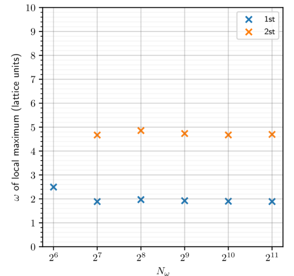
To produce the glueball spectra given in section 3.2, $\omega$ was sampled evenly in logarithmic space between $[10^{-5},10^{5}]$ $\text{\,}\mathrm{GeV}$, in $N_{\omega}=2000$ steps, when constructing the Laplace kernel $\boldsymbol{K}$. However, this number of steps $N_{\omega}$ is unnecessarily large, and was chosen merely to generate aesthetically pleasing graphs.

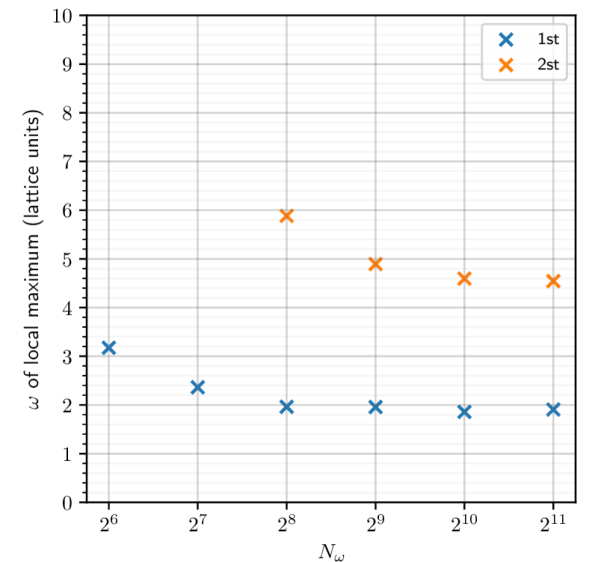
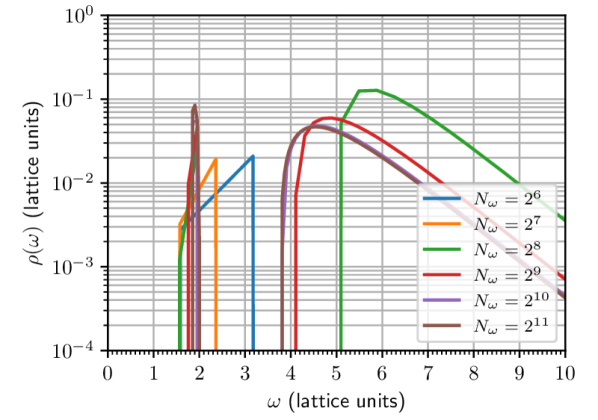
To demonstrate the convergence of the maxima of the spectral functions, fig. 7 shows the $\omega$ coordinate of the first and second maximum in the $\beta=2.1$ data set for increasing $N_{\omega}$. In both the linearly spaced and logarithmically evenly spaced scenarios, the ground state converges rapidly, and the second maximum soon follows suit. In addition, fig. 8 shows the full spectrum in both scenarios. There is excellent agreement between the two methods for the determination of the ground state mass, but the overall convergence is better when using logarithmically evenly spaced samples.

(a) Results for logarithmic sample of $\omega$ in $[10^{-5},10^{5}]$ $\text{\,}\mathrm{GeV}$.

(b) Results for linear sample of $\omega$ in $[0,100]$ $\text{\,}\mathrm{GeV}$.

Figure 7: The position of the first and second maxima for the $\beta=2.1$ data set, as a function of the number of samples $N_{\omega}$ in the Laplace kernel $\boldsymbol{K}$.

(a) $\omega$ sampled uniformly in logarithmic space between $[10^{-5},10^{5}]$ $\text{\,}\mathrm{GeV}$.

(b) $\omega$ sampled uniformly in linear space between $[0,100]$ $\text{\,}\mathrm{GeV}$.

Figure 8: $\rho(\omega)$ for the $\beta=2.1$ data set, as a function of the number of samples $N_{\omega}$ in the Laplace kernel $\boldsymbol{K}$.

References

- [1] N. Yamanaka, H. Iida, A. Nakamura and M. Wakayama “Glueball scattering cross section in lattice SU(2) Yang-Mills theory” In Phys. Rev. D 102.5, 2020, pp. 054507 DOI: 10.1103/PhysRevD.102.054507
- [2] P.. Zyla “Review of Particle Physics” In PTEP 2020.8, 2020, pp. 083C01 DOI: 10.1093/ptep/ptaa104
- [3] M. Teper “Glueball masses and other physical properties of SU(N) gauge theories in D = (3+1): A Review of lattice results for theorists”, 1998 arXiv:hep-th/9812187
- [4] C.. Morningstar and M.. Peardon “The Glueball spectrum from an anisotropic lattice study” In Phys. Rev. D 60, 1999, pp. 034509 DOI: 10.1103/PhysRevD.60.034509
- [5] Y. Chen “Glueball spectrum and matrix elements on anisotropic lattices” In Phys. Rev. D 73, 2006, pp. 014516 DOI: 10.1103/PhysRevD.73.014516
- [6] S. Narison “Masses, decays and mixings of gluonia in QCD” In Nucl. Phys. B 509, 1998, pp. 312–356 DOI: 10.1016/S0550-3213(97)00562-2
- [7] R.. Brower, S.. Mathur and C.-I. Tan “Glueball spectrum for QCD from AdS supergravity duality” In Nucl. Phys. B 587, 2000, pp. 249–276 DOI: 10.1016/S0550-3213(00)00435-1
- [8] N. Ishii, H. Suganuma and H. Matsufuru “Glueball properties at finite temperature in SU(3) anisotropic lattice QCD” In Phys. Rev. D 66, 2002, pp. 094506 DOI: 10.1103/PhysRevD.66.094506
- [9] A.. Szczepaniak and E.. Swanson “The Low lying glueball spectrum” In Phys. Lett. B 577, 2003, pp. 61–66 DOI: 10.1016/j.physletb.2003.10.008
- [10] D. Dudal, M.. Guimaraes and S.. Sorella “Glueball masses from an infrared moment problem and nonperturbative Landau gauge” In Phys. Rev. Lett. 106, 2011, pp. 062003 DOI: 10.1103/PhysRevLett.106.062003
- [11] H. Sanchis-Alepuz, C.. Fischer, C. Kellermann and L. Smekal “Glueballs from the Bethe-Salpeter equation” In Phys. Rev. D 92, 2015, pp. 034001 DOI: 10.1103/PhysRevD.92.034001
- [12] M.. Huber, C.. Fischer and H. Sanchis-Alepuz “Spectrum of scalar and pseudoscalar glueballs from functional methods” In Eur. Phys. J. C 80.11, 2020, pp. 1077 DOI: 10.1140/epjc/s10052-020-08649-6
- [13] V. Mathieu, N. Kochelev and V. Vento “The Physics of Glueballs” In Int. J. Mod. Phys. E 18, 2009, pp. 1–49 DOI: 10.1142/S0218301309012124
- [14] V. Crede and C.. Meyer “The Experimental Status of Glueballs” In Prog. Part. Nucl. Phys. 63, 2009, pp. 74–116 DOI: 10.1016/j.ppnp.2009.03.001
- [15] W. Ochs “The Status of Glueballs” In J. Phys. G 40, 2013, pp. 043001 DOI: 10.1088/0954-3899/40/4/043001
- [16] A.. Sarantsev, I. Denisenko, U. Thoma and E. Klempt “Scalar isoscalar mesons and the scalar glueball from radiative decays” In Phys. Lett. B 816, 2021, pp. 136227 DOI: 10.1016/j.physletb.2021.136227
- [17] M.. Hertzberg, F. Rompineve and J. Yang “Decay of Boson Stars with Application to Glueballs and Other Real Scalars” In Phys. Rev. D 103.2, 2021, pp. 023536 DOI: 10.1103/PhysRevD.103.023536
- [18] K. Ishikawa, M. Teper and G. Schierholz “The Glueball Mass Spectrum in QCD: First Results of a Lattice Monte Carlo Calculation” In Phys. Lett. B 110, 1982, pp. 399–405 DOI: 10.1016/0370-2693(82)91281-3
- [19] I. Montvay and G. Munster “Quantum fields on a lattice”, Cambridge Monographs on Mathematical Physics Cambridge University Press, 1997 DOI: 10.1017/CBO9780511470783
- [20] L. Maiani and M. Testa “Final state interactions from Euclidean correlation functions” In Phys. Lett. B 245, 1990, pp. 585–590 DOI: 10.1016/0370-2693(90)90695-3
- [21] L. Lellouch and M. Luscher “Weak transition matrix elements from finite volume correlation functions” In Commun. Math. Phys. 219, 2001, pp. 31–44 DOI: 10.1007/s002200100410
- [22] M.. Peskin and D.. Schroeder “An Introduction to quantum field theory” Reading, USA: Addison-Wesley, 1995 URL: http://www.slac.stanford.edu/~mpeskin/QFT.html
- [23] B. Blossier, M. Della Morte, G. Hippel, T. Mendes and R. Sommer “On the generalized eigenvalue method for energies and matrix elements in lattice field theory” In JHEP 04, 2009, pp. 094 DOI: 10.1088/1126-6708/2009/04/094
- [24] A. Athenodorou and M. Teper “The glueball spectrum of SU(3) gauge theory in 3 + 1 dimensions” In JHEP 11, 2020, pp. 172 DOI: 10.1007/JHEP11(2020)172
- [25] J.. Negele and H. Orland “Quantum Many Particle Systems” Redwood City, USA: Addison-Wesley. (Frontiers in Physics, 68), 1988
- [26] H.. Meyer “Transport Properties of the Quark-Gluon Plasma: A Lattice QCD Perspective” In Eur. Phys. J. A47, 2011, pp. 86 DOI: 10.1140/epja/i2011-11086-3
- [27] D. Dudal and M.. Guimaraes “On the computation of the spectral density of two-point functions: complex masses, cut rules and beyond” In Phys. Rev. D 83, 2011, pp. 045013 DOI: 10.1103/PhysRevD.83.045013
- [28] D. Dudal, O. Oliveira and P.. Silva “Källén-Lehmann spectroscopy for (un)physical degrees of freedom” In Phys. Rev. D 89.1, 2014, pp. 014010 DOI: 10.1103/PhysRevD.89.014010
- [29] E.. Solis, C… Costa, V.. Luiz and G. Krein “Quark propagator in Minkowski space” In Few Body Syst. 60.3, 2019, pp. 49 DOI: 10.1007/s00601-019-1517-9
- [30] D. Dudal et al. “Some remarks on the spectral functions of the Abelian Higgs Model” In Phys. Rev. D 100.6, 2019, pp. 065009 DOI: 10.1103/PhysRevD.100.065009
- [31] D. Binosi and R.-A. Tripolt “Spectral functions of confined particles” In Phys. Lett. B 801, 2020, pp. 135171 DOI: 10.1016/j.physletb.2019.135171
- [32] F. Siringo “Analytic structure of QCD propagators in Minkowski space” In Phys. Rev. D 94.11, 2016, pp. 114036 DOI: 10.1103/PhysRevD.94.114036
- [33] A.. Cyrol, J.. Pawlowski, A. Rothkopf and N. Wink “Reconstructing the gluon” In SciPost Phys. 5, 2018, pp. 065 DOI: 10.21468/SciPostPhys.5.6.065
- [34] S. Weinberg “The Quantum Theory of Fields” Cambridge University Press, 1995 DOI: 10.1017/CBO9781139644167
- [35] O. Oliveira, D. Dudal and P.. Silva “Glueball spectral densities from the lattice” In PoS LATTICE2012, 2012, pp. 214 DOI: 10.22323/1.164.0214
- [36] D. Dudal, O. Oliveira, M. Roelfs and P. Silva “Spectral representation of lattice gluon and ghost propagators at zero temperature” In Nucl. Phys. B 952, 2020, pp. 114912 DOI: 10.1016/j.nuclphysb.2019.114912
- [37] C.. Lawson, Society for Industrial Hanson and Applied Mathematics “Solving least squares problems” Philadelphia : SIAM, 1995 URL: http://www.loc.gov/catdir/enhancements/fy0617/95035178-t.html
- [38] M. Asakawa, T. Hatsuda and Y. Nakahara “Maximum entropy analysis of the spectral functions in lattice QCD” In Prog. Part. Nucl. Phys. 46, 2001, pp. 459–508 DOI: 10.1016/S0146-6410(01)00150-8
- [39] G. Aarts, C. Allton, M.. Oktay, M. Peardon and J.-I. Skullerud “Charmonium at high temperature in two-flavor QCD” In Phys. Rev. D 76, 2007, pp. 094513 DOI: 10.1103/PhysRevD.76.094513
- [40] A. Jakovac, P. Petreczky, K. Petrov and A. Velytsky “Quarkonium correlators and spectral functions at zero and finite temperature” In Phys. Rev. D 75, 2007, pp. 014506 DOI: 10.1103/PhysRevD.75.014506
- [41] A. Rothkopf “Bayesian inference of nonpositive spectral functions in quantum field theory” In Phys. Rev. D 95.5, 2017, pp. 056016 DOI: 10.1103/PhysRevD.95.056016
- [42] H.-T. Ding, O. Kaczmarek, S. Mukherjee, H. Ohno and H. Shu “Stochastic reconstructions of spectral functions: Application to lattice QCD” In Phys. Rev. D 97.9, 2018, pp. 094503 DOI: 10.1103/PhysRevD.97.094503
- [43] R.-A. Tripolt, P. Gubler, M. Ulybyshev and L. Von Smekal “Numerical analytic continuation of Euclidean data” In Comput. Phys. Commun. 237, 2019, pp. 129–142 DOI: 10.1016/j.cpc.2018.11.012
- [44] S. Schlichting, D. Smith and L. Smekal “Spectral functions and critical dynamics of the model from classical-statistical lattice simulations” In Nucl. Phys. B 950, 2020, pp. 114868 DOI: 10.1016/j.nuclphysb.2019.114868
- [45] R. Fournier, L. Wang, O.. Yazyev and Q. Wu “Artificial Neural Network Approach to the Analytic Continuation Problem” In Phys. Rev. Lett. 124 American Physical Society, 2020, pp. 056401 DOI: 10.1103/PhysRevLett.124.056401
- [46] Pauli Virtanen et al. “SciPy 1.0: Fundamental Algorithms for Scientific Computing in Python” In Nature Methods 17, 2020, pp. 261–272 DOI: 10.1038/s41592-019-0686-2
- [47] A. Kirsch “An Introduction to the Mathematical Theory of Inverse Problems” Berlin, Heidelberg: Springer-Verlag, 1996
- [48] Martin Roelfs and Peter C Kroon “tBuLi/symfit: symfit 0.5.4” Zenodo, 2021 DOI: 10.5281/zenodo.5519611
- [49] N. Yamanaka, H. Iida, A. Nakamura and M. Wakayama “Dark matter scattering cross section and dynamics in dark Yang-Mills theory” In Phys. Lett. B 813, 2021, pp. 136056 DOI: 10.1016/j.physletb.2020.136056
- [50] Andreas Athenodorou and Michael Teper “SU(N) gauge theories in 3+1 dimensions: glueball spectrum, string tensions and topology” In JHEP 12, 2021, pp. 082 DOI: 10.1007/JHEP12(2021)082
- [51] A.. Kataev, N.. Krasnikov and A.. Pivovarov “Two Loop Calculations for the Propagators of Gluonic Currents” [Erratum: Nucl.Phys.B 490, 505–507 (1997)] In Nucl. Phys. B 198, 1982, pp. 508–518 DOI: 10.1016/0550-3213(82)90338-8