Large Motion Video Super-Resolution with Dual Subnet and Multi-Stage Communicated Upsampling

Abstract

Video super-resolution (VSR) aims at restoring a video in low-resolution (LR) and improving it to higher-resolution (HR). Due to the characteristics of video tasks, it is very important that motion information among frames should be well concerned, summarized and utilized for guidance in a VSR algorithm. Especially, when a video contains large motion, conventional methods easily bring incoherent results or artifacts. In this paper, we propose a novel deep neural network with Dual Subnet and Multi-stage Communicated Upsampling (DSMC) for super-resolution of videos with large motion. We design a new module named U-shaped residual dense network with 3D convolution (U3D-RDN) for fine implicit motion estimation and motion compensation (MEMC) as well as coarse spatial feature extraction. And we present a new Multi-Stage Communicated Upsampling (MSCU) module to make full use of the intermediate results of upsampling for guiding the VSR. Moreover, a novel dual subnet is devised to aid the training of our DSMC, whose dual loss helps to reduce the solution space as well as enhance the generalization ability. Our experimental results confirm that our method achieves superior performance on videos with large motion compared to state-of-the-art methods.

Introduction

Video super-resolution (VSR) aims at recovering the corresponding high-resolution (HR) counterpart from a given low-resolution (LR) video (Liu et al. 2020b). As an important computer vision task, it is a classic ill-posed problem. In recent years, due to the emergence of 5G technology and the popularity of high-definition (HD) and ultra high-definition (UHD) devices (Liu et al. 2020a), the VSR technology has attracted more attention from researchers and has become one of the research spotlights. Traditional super-resolution (SR) methods mainly include interpolation, statistical methods and sparse representation methods.

In recent years, with the rapid development of deep neural networks, deep-learning-based VSR has attracted more attention among researchers. Due to the powerful data fitting and feature extraction ability, such algorithms are generally superior to traditional super-resolution techniques. The first deep-learning-based single image super-resolution (SISR) algorithm is SRCNN (Dong et al. 2015), while the first deep-learning-based VSR algorithm is Deep-DE (Liao et al. 2015). Since then, many deep-learning-based VSR algorithms have been proposed, such as VSRnet (Kappeler et al. 2016), 3DSRNet (Kim et al. 2018), RBPN (Haris, Shakhnarovich, and Ukita 2019) and TDAN (Tian et al. 2020). It may be considered that VSR can be achieved by using SISR algorithms frame by frame. However, SISR algorithms ignore temporal consistency between frames and easily brings artifact and jam, leading to worse visual experience. In contrast, VSR methods are usually able to process such consecutive frames and generate HR video with more natural details and less artifact.

There are many VSR methods based on motion estimation and motion compensation (MEMC). They rely heavily on optical flow estimation for consecutive frames, and thus execute compensation to import temporal information to the center frame. For example, SOF-VSR (Wang et al. 2018a) proposed a coarse-to-fine CNN to gradually estimate HR optical flow in three stages. And RBPN (Haris, Shakhnarovich, and Ukita 2019) presented a back projection module which is composed of a sequence of consecutive alternate encoders and decoders after implicit alignment. They work well for videos consisting of scenes with small motion in a short time, as the optical flow estimation is accurate under such ideal scenes. However, in actual multimedia scenes, the motion are always diverse in different amplitudes. Especially when real-time shooting scenes like extreme sports have been popular, wearable shooting equipments can be widely used and often bring about video jitter. The jitter can easily bring about large motions. In visual tasks, large motion is always based on the consistency assumption of optical flow calculation (Gibson 1957). If the target motion changes too fast relative to the frame rate, this motion can be called large motion in videos.

Moreover, some VSR methods do not perform explicit MEMC. They directly input multiple frames for spatio-temporal feature extraction, fusion and super-resolution, thus achieve implicit MEMC. For example, 3DSRNet (Kim et al. 2018) and FSTRN (Li et al. 2019) utilize 3D convolution (C3D) (Ji et al. 2012) to extract spatio-temporal correlation on the spatio-temporal domain. However, high computational complexity of C3D limits them to develop deeper structures. This probably results in their limited modeling and generalization ability, and the difficulty to adapt to videos with large motion.

To address the above challenges, we propose a novel video super-resolution network with Dual Subnet and Multi-stage Communicated Upsampling (DSMC) to maximize the communication of various decisive information for videos with large motion. DSMC receives a center LR frame and its neighboring frames for each SR. After coarse-to-fine spatial feature extraction on the input frames, a U-shaped residual dense network with 3D convolution (U3D-RDN) is designed for DSMC. It can encode the input features and achieve both fine implicit MEMC and coarse spatial feature extraction on the encoding space as well as reducing the computational complexity. Then U3D-RDN decodes the features by a sub-pixel convolution upsampling layer. After another fine spatial feature extraction, a Multi-Stage Communicated Upsampling (MSCU) module is proposed to decompose an upsampling into multiple sub-tasks. It conducts feature correction with the help of the VSR result from each sub task, and thus makes full use of the intermediate results of upsampling for VSR guidance. Finally, a dual subnet is presented and used to simulate degradation of natural image, and the dual loss between the degraded VSR result and the original LR frame is computed to aid the training of DSMC.

The main contributions of this paper are as follows:

• We propose a DSMC network for super-resolution of videos with large motion, which is designed to maximize the communication of various decisive information in VSR process and implicitly capture the motion information. Our DSMC can guide the upsampling process with more sufficient prior knowledge than other state-of-the-art ones by the proposed MSCU model. Meanwhile, the proposed U3D-RDN module can learn coarse-to-fine spatio-temporal features from the input video frames, and therefore effectively guide VSR process for large motion.

• We propose a dual subnet for our DSMC, which can simulate natural image degradation to reduce the solution space, enhance the generalization ability and help DSMC for better training.

• Extensive experiments have been carried out to evaluate the proposed DSMC. We compare it with several state-of-the-art methods including optical-flow-based and C3D-based ones. Experimental results confirm that DSMC is effective for videos with large motion as well as for generic videos without large motion.

• Ablation study for each individual design has been conducted to investigate the effectiveness of our DSMC. We can find that MSCU has the greatest influence on the performance as it can recover more details through multi-stage communication. U3D-RDN is also effective for extracting motion information. The ablation study also indicates that the loss functions in dual subnet influence the training of DSMC when the original loss function is under different combinations of Cb and perceptual losses.

Related Work

SISR Methods Based on Deep Learning

Recently, with the development of deep learning, super-resolution algorithms based on deep learning usually perform much better than traditional methods in terms of various evaluation indicators, such as PSNR and SSIM. The first deep-learning-based SISR algorithm (called SRCNN) was proposed by Dong et al. (2015). It consists of three convolutional layers and learns a non-linear mapping from LR images to HR images by an end-to-end manner. Since then, many deep learning methods have been transferred to SISR, which help subsequent methods obtain greater performance.

Inspired by VGG (Simonyan and Zisserman 2014), some methods generally adopt deeper network architecture, such as VDSR (Kim, Kwon Lee, and Mu Lee 2016), EDSR (Lim et al. 2017) and RCAN (Zhang et al. 2018a). However, these methods may suffer from gradient vanishment problem. Therefore, many algorithms such as RDN (Zhang et al. 2018b) introduce the skip connection between different layers inspired by the residual network (ResNet) (He et al. 2016b). In addition, the input size of SRCNN is the same as ground truth, which can lead to a high computational complexity. Therefore, most subsequent algorithms adopt a single LR image as input and execute upsampling on it at the end of the network, such as ESPCN (Shi et al. 2016) and DRN (Guo et al. 2020). Besides, other strategies such as attention mechanism (Mnih et al. 2014), non-local (Wang et al. 2018b) and dense connection (Huang et al. 2017) are also introduced to enhance the performance of SISR methods.

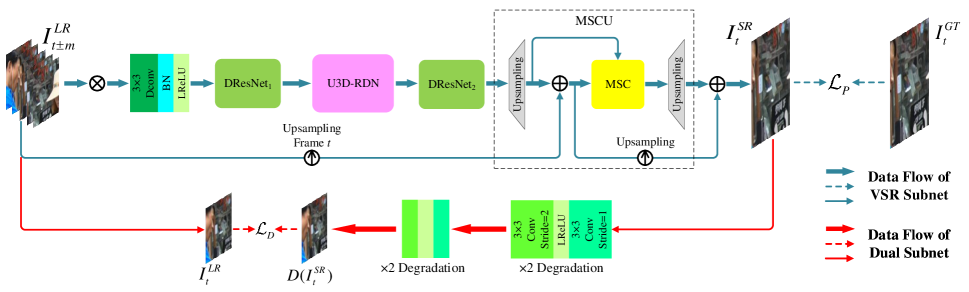
Figure 1: The architecture of the proposed DSMC method. $I_{t\pm m}^{LR}$ denotes the input frames, ’$\otimes$’ denotes channel-wise concatenation, ’$\oplus$’ denotes element-wise addition, D($\cdot$) is the dual subnet, and MSC is short for Multi-Stage Communication.

VSR Methods Based on Deep Learning

The earliest application of deep learning to VSR can be traced back to Deep-DE proposed by Liao et al. (2015). Since then, more advanced VSR methods have been proposed, such as VSRnet (Kappeler et al. 2016), VESPCN (Caballero et al. 2017), SOF-VSR (Wang et al. 2018a), RBPN (Haris, Shakhnarovich, and Ukita 2019), and 3DSRNet (Kim et al. 2018).

For the VSR methods using 2D convolution, explicit MEMC is widely used and studied. VSRnet used the Druleas algorithm (Drulea and Nedevschi 2011) to calculate optical flows. In addition, the authors also proposed a filter symmetry mechanism and adaptive motion compensation to accelerate training and reduce the impact of unreliable motion compensated frames. However, the architecture of VSRnet is still relatively simple. Therefore, most recently proposed VSR methods tend to use more complicated explicit MEMC architectures for capturing motion information. Caballero et al. (2017) proposed space converter based on CNN for explicit MEMC. Xue et al. (2019) utilized SpyNet (Ranjan and Black 2017) to estimate optical flows, which were transformed to neighboring frames by a space transformation network (Jaderberg et al. 2015). Kalarot and Porikli (2019) aligned frames through FlowNet 2.0 (Ilg et al. 2017). Wang et al. (2018a) proposed a coarse-to-fine CNN to gradually estimate HR optical flow in three stages. Sajjadi, Vemulapalli, and Brown (2018) tried to warp the VSR results rather than LR inputs. Haris, Shakhnarovich, and Ukita (2019) presented a back projection module, which is composed of a sequence of alternate encoders and decoders after implicit alignment. And Xin et al. (2020) proposed a motion-adaptive feedback cell, which can throw away the redundant information to help useful motion compensation. These methods have achieved better perceptual quality than traditional methods (e.g. bicubic interpolation) and SISR methods with less computational complexity. However, they only work well for videos consisting of scenes with small motion in a short time and less lighting variation. If LR videos are with large motion or significant lighting changes, the performance of explicit MEMC-based methods always degrades greatly.

3D convolution (C3D) can free VSR from explicit MEMC by adding an extra dimensionality. Therefore, C3D-based VSR methods can process videos with various lighting and motion, which enhances their practicability. Existing studies of C3D in VSR are relatively few. Kim et al. (2018) use extrapolation operation, which can be understood as the padding operation in temporal domain. Li et al. (2019) decomposed the general C3D kernels to lower dimensions to reduce computational complexity. Jo et al. (2018) proposed a dynamic upsampling filter structure inspired by dynamic filter networks (Jia et al. 2016), which can combine the spatio-temporal information learned by C3D to generate corresponding filters for specific inputs. In order to enhance high-frequency details, an additional network is used to estimate the residual maps. Ying et al. (2020) proposed a deformable variant of C3D. However, the balance of performance and high computational complexity is still an unsolved challenge which restrains wider application of C3D-based VSR methods.

Proposed Method

Network Architecture

In this subsection, we give a brief description to the proposed DSMC. It is designed to maximize the communication of various decisive information, so as to maintain excellent robustness in large motion. DSMC includes a VSR subnet (feature extraction and Multi-Stage Communiated Upsampling (MSCU)) and a dual subnet. It uses a center LR frame and $2m$ neighboring frames $I_{t\pm m}^{LR}$ as inputs, and outputs a super-resolved HR frame $I_{t}^{SR}$. The overall objective function can be formulated as follows:

$$I_{t}^{SR}=H_{DSMC}(I)$$ (1)

where $H_{DSMC}(\cdot)$ is our DSMC, and $I$ is a LR frame window defined as

$$I=[I_{t-m}^{LR},I_{t-m+1}^{LR},\dots,I_{t}^{LR},\dots,I_{t+m-1}^{LR},I_{t+m}^{LR}]$$ (2)

where $t$ is the position of the center frame and $m$ is the relative offset of neighboring frames.

The architecture of the proposed DSMC is shown in Figure 1. In details, taking a $\times 4$ VSR task as an example, our model firstly performs deformable convolution on the input consecutive frames for coarse feature extraction. The output feature maps are then processed by a deformable residual network (DResNet) (Lei and Todorovic 2018) to extract fine spatial information before considering temporal features. Next, the feature maps are input to the U-shaped residual dense network with 3D convolution (U3D-RDN) for dimension reduction and correlation analyzation of spatio-temporal feature. Followed by another DResNet module, the feature maps are sent to a Multi-Stage Communicated Upsampling (MSCU) module. Finally, with the aid of a dual subnet for training, DSMC yields the super-resolved HR frames. It is noted that only the output of the dual subnet, $D(I^{SR}_{t})$, and the VSR result, $I^{SR}_{t}$, are used for the loss computation of DSMC.

In the following subsections, we will give detailed analysis on the motivation and rationality of each module in the proposed DSMC.

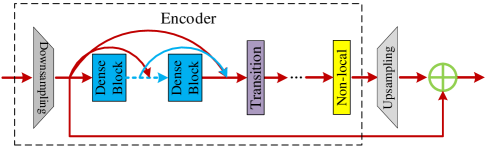
Figure 2: The U3D-RDN module for our DSMC.

U3D-RDN

We firstly propose a new U-shaped residual dense network with 3D convolution (U3D-RDN) for our DSMC to achieve both fine implicit MEMC and coarse spatial feature extraction as well as reducing computational complexity, as shown in Figure 2. As it is known, DenseNet (Huang et al. 2017) has achieved sound performance in many deep learning applications. Then Zhang et al. (2018b) proposed a design of residual dense network (ResDenseNet) making full use of the hierarchical features of the LR input in SISR. Unlike the previous work, U3D-RDN is able to execute implicit MEMC without a high computational complexity. It encodes the input features by $\times 2$ downsampling with a $3\times 3$ 2D convolution, and then decodes the residual maps by a sub-pixel convolution upsampling layer after residual learning on the encoding space.

The proposed module is explained in details below. It consists of $m$ groups of dense blocks with 3D convolution (3D DenseBlock), as shown in Figure 3 (a), transition layers in Figure 3 (b) among the groups, and a 3D non-local (Wang et al. 2018b) layer. Our 3D DenseBlock uses 3D convolution (C3D) to avoid the shortage of optical-flow-based methods on videos with large motion, which operates in both spatial and temporal domains of the input features. In a 3D DenseBlock, the $1\times 1\times 1$ C3D is responsible for feature decomposition of the input, while the $3\times 3\times 3$ C3D is for the spatio-temporal feature extraction in the high-dimensional space. These groups of blocks can together establish long-distance dependence and avoid the gradient vanishing problem. The output of the $i$-th group of 3D DenseBlock is expressed as

$$\mathcal{D}_{i}(I)=d_{i}^{L}([d_{i}^{0}(I),d_{i}^{1}(I),\dots,d_{i}^{L-1}(I)])$$ (3)

where $d_{i}^{l}(\cdot),l\in(1,\dots,L)$ is the $l$-th 3D DenseBlock in the $i$-th group, and $L$ is the number of the block in each group.

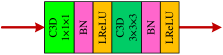
(a) A 3D DenseBlock

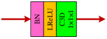
(b) A transition layer

Figure 3: Details of the proposed U3D-RDN module.

In our U3D-RDN, a transition layer is deployed after each 3D DenseBlock except for the last one. It can halve the temporal dimension of the previous group of cascaded outputs to enhance the learning ability of the module and help realize a deeper network. As it is known, when the number of 3D DenseBlock increases, the dimensions entered by adjacent blocks grow too. Then the learning ability of U3D-RDN can also be enhanced as the network goes deeper. However, the rise of depth also induces a burden on hardware costs. Transition layers can sustain the increase of network depth and relieve the burden of computational costs.

Moreover, the C3D may highlight the shortage of long-distance dependence in CNN due to its synchronous spatio-temporal process. Therefore, before upsampling the output of 3D DenseBlock, a non-local module is adopted to process the feature maps. This non-local module can establish a more relevant dependence on global information.

In summary, the process of U3D-RDN module is given by

$$\mathcal{R}(I)=\mathcal{N}(\mathcal{D}_{m}(I)){\uparrow_{s}}+\mathcal{H}(I)$$ (4)

where $\mathcal{R}(\cdot)$ is the output, $\mathcal{N}(\cdot)$ is the non-local module, ’$\uparrow_{s}$’ is sub-pixel convolution, and $\mathcal{H}$ is the inputs of U3D-RDN.

Multi-Stage Communicated Upsampling

We also propose a novel Multi-Stage Communicated Upsampling (MSCU) module to make full use of the prior knowledge in upsampling stages for restoring HR frames. The architecture of MSCU is shown in Figure 4. The curse of dimensionality is considered to be the main factor restricting super-resolution. If the mapping from LR to HR space is directly established, a poor super-resolution algorithm will lack sufficient prior information with the increase of scale factor, causing the distortion of results. In general, there are many sources of prior information. For example, in residual learning, the residual information of the upsampled image after interpolation is used for learning. As shown in (He et al. 2016b), residual learning usually achieves superior performance. Thus the interpolated image can be a type of prior knowledge, which is not available in a super-resolution network that directly learns HR results.

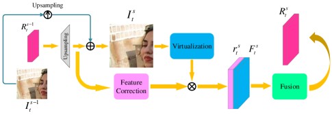
Figure 4: One stage of the proposed MSCU module.

In our MSCU, in order to take full advantage of prior information, we decompose the upsampling process of VSR to smaller ones. We suggest that each sub scale factor should be in prime to maximize the communication ability of the structure. For example, a $\times 4$ upsampling task can be decomposed into two consecutive $\times 2$ upsampling tasks. Through the sub-outputs, the network will be able to capture the corresponding uncertainties in each stage and try fixing them. The residual maps after upsampling proceed to two branches. One is the feature correction by a ResNet to generate $r_{t}^{s}$, while the other is the channel reduction by a $1\times 1$ convolution and the element-wise addition with the bicubic-upsampled center frame to generate the fixed frame $I_{t}^{s}$. Then $I_{t}^{s}$ will be virtualized by another $1\times 1$ convolution. The virtual results $F_{t}^{s}$ are next channel-wise concatenated to $r_{t}^{s}$. The concatenated feature maps are finally fused by a $1\times 1$ convolution to generate residual maps $R_{t}^{s}$ for the next stage. The above process can be summarized as follows:

$$R_{t}^{s}=\mathcal{G}([r_{t}^{s},F_{t}^{s}])$$ (5)

where

$$r_{t}^{s}=\mathcal{H}_{0}((R_{t}^{s-1})_{\uparrow})$$ (6)

$$F_{t}^{s}=\mathcal{V}(I_{t}^{s})$$ (7)

$$I_{t}^{s}=(I_{t}^{s-1})_{\uparrow}+(R_{t}^{s-1})_{\uparrow s}$$ (8)

Besides, $s\in\{1,2,\dots,S-1\}$, $S$ is the number of stages, $\mathcal{G}(\cdot)$ is channel fusion, $\mathcal{H}_{0}(\cdot)$ is the feature correction network, $\mathcal{V}(\cdot)$ is visulization, and ’$\uparrow$’ is bicubic upsampling.

Therefore, the equation (1) is equivalent to

$$I_{t}^{SR}=(I_{t}^{S-1})_{\uparrow}+(R_{t}^{S-1})_{\uparrow s}$$ (9)

Dual Subnet

We design a novel dual subnet for our DSMC to constrain the solution space. To the best of our knowledge, it is the first design of dual learning in VSR. The architecture of our DSMC with the subnet is shown in Figure 1. The reason that the dual learning mechanism (He et al. 2016a) works is the multi-task connectivity of collaborative operations. It can extend the training constraints to both the outputs and the inputs, which helps to further reduce the solution space and thus makes the network easier to converge.

The purpose of VSR is to map LR frames to their corresponding HR space. Therefore, the dual problem is to restore the degradation results of the VSR outputs as close as possible to the LR target frame. In our proposed dual subnet, we simulate the real image degradation process, which consists of blur, downsampling and noise addition. Mathematically, the SR image $I^{SR}$ and LR image $I^{LR}$ are related by the following degradation model (Gu et al. 2019):

$$I^{LR}=({I^{SR}}\otimes k)_{\downarrow s}+n$$ (10)

where $k$ denotes the blur kernel, ${\downarrow s}$ is downsampling process, and $n$ is the added noise. Specifically, the blur and downsampling processes are separately completed by two $3\times 3$ 2D convolutions (C2Ds), while the noise is added to the degraded frame by the bias of the downsampling C2D.

Note that the dual subnet is proposed for helping DSMC converge to a better solution. In our dual learning, the dual loss $\mathcal{L}_{D}$ is computed between the input frame $I_{t}^{LR}$ and the output of the dual subnet. Then the total training loss $\mathcal{L}$ of DSMC is composed of two parts: the original loss $\mathcal{L}_{P}$ from the VSR subnet and $\mathcal{L}_{D}$, given as follows:

$$\mathcal{L}=\sum_{t=1}^{N}[{\lambda}_{1}\mathcal{L}_{P}(I_{t}^{SR},I_{t}^{GT})+{\lambda}_{2}\mathcal{L}_{D}(D(I_{t}^{SR}),I_{t}^{LR})]$$ (11)

where $I_{t}^{GT}$ is the ground truth, $D$ is the dual subnet with $I_{t}^{SR}$ as input, ${\lambda}_{i},i\in\{1,2\}$ are constants which represent the weight of the two losses, and $N$ is the number of frames.

In fact, we can adopt widely-used Mean Square Error (MSE), Charbonnier (Cb), or perceptual loss for calculating $\mathcal{L}_{P}$ and $\mathcal{L}_{D}$. Nevertheless, studies indicate that more strict dual mechanism can better recover the reverse process of the original task. Therefore, we suggest that $\mathcal{L}_{P}$ and $\mathcal{L}_{D}$ should use the same loss function to restrain both $I^{LR}$ and $I^{SR}$ to the same distribution. For instance, if $\mathcal{L}_{P}$ consists of multiple types of losses (e.g. Cb and perceptual loss) with different effects, then $\mathcal{L}_{D}$ should also include these losses.

Experiments

Datasets and Metrics

In our experiments, we use REDS (Nah et al. 2019) in RGB channels as the training dataset. It contains 240 videos (100 frames for each) for training and 30 videos (100 frames for each) for validation, which are all recorded by GoPro camera in a variety of scenes. As many videos contain large motion, they are challenging for frame alignment. Then we evaluate the performance of our DSMC for VSR tasks on the REDS4 and Vid4 datasets. REDS4 consists of 4 typical videos selected from the REDS validation set, while Vid4 is a benchmark dataset widely used in VSR. All the above datasets are for the $\times 4$ VSR task. To obtain LR videos from the Vid4 benchmark dataset, we downsample HR videos with the scaling factor $\times 4$ by bicubic interpolation. For each dataset except Vid4, we randomly crop frame patches with the LR size of $64\times 64$ as inputs and ground truths (GTs). The mini-batch size during training is set to 8. For data augmentation, we perform randomly horizontal flip and 90 degree rotation. And we evaluate the performance on RGB channels by two most common metrics: peak signal-to-noise ratio (PSNR) and structure similarity index (SSIM).

Table 1: PSNR/SSIM results of different methods on the REDS4 dataset for scale factor $\times 4$. $Params.$ is short for the number of parameters ($\times 10^{6}$). All the metrics are compared on RGB channels. Note that the the best results are in red boldface and the second best results are in blue boldface.

Clip Name	Bicubic	SRCNN	DBPN	VESPCN	SOF-VSR	3DSRnet	RBPN	DRVSR	FRVSR	DSMC (ours)
Clip_000	24.83/0.8076	25.88/0.8443	27.24/0.8831	26.57/0.8649	26.82/0.8722	25.30/0.8230	27.10/0.8785	26.53/0.8640	26.98/0.8776	27.56/0.8934
Clip_011	21.60/0.7061	22.61/0.7628	23.12/0.7859	22.89/0.7753	22.97/0.7785	22.16/0.7399	23.04/0.7812	22.84/0.7722	23.23/0.7901	23.57/0.8070
Clip_015	21.12/0.6687	21.88/0.7236	22.46/0.7543	22.08/0.7378	22.22/0.7445	21.66/0.7116	22.28/0.7479	22.10/0.7379	22.63/0.7676	23.11/0.7897
Clip_020	27.33/0.8412	27.91/0.8584	28.29/0.8673	28.18/0.8648	28.21/0.8668	27.88/0.8554	28.25/0.8671	28.15/0.8643	28.25/0.8671	28.68/0.8810
Average	23.72/0.7559	24.57/0.7973	25.28/0.8227	24.93/0.8107	25.05/0.8155	24.25/0.7825	25.17/0.8187	24.90/0.8096	25.27/0.8256	25.73/0.8428
Params.	-	0.07M	10.42M	0.88M	1.71M	0.11M	14.51M	2.17M	2.81M	11.58M

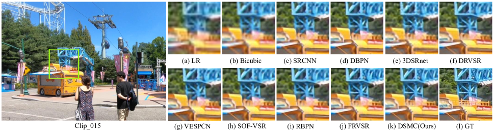
Figure 5: Qualitative results by different methods on the REDS4 dataset.

Implementation Details

Our DSMC uses 5 consecutive frames as the inputs. For the beginning and the end frames that do not have enough frames in the window, we pad with different Gaussian-blured center frames with $radius=0.1d$ ($d$ is the distance from center to the padding) to simulate the focusing and defocusing of camera. $\alpha$ is set to 0.1 in the LReLUs of the whole network. In U3D-RDN, the number of the groups of 3D DenseBlocks $m$ is set to 4, and the sizes which represent the number of 3D DenseBlocks in each group are set to (2, 6, 6, 3), respectively. Our model is trained by the Adam optimizer with the momentum parameter $\beta_{1}=0.9$. The loss function is defined in Equation (11), where ${\lambda}_{1}=1$ and ${\lambda}_{2}=0.1$, $\mathcal{L}_{P}$ and $\mathcal{L}_{D}$ are of the Cb loss (Cui et al. 2019) and perceptual loss (Johnson, Alahi, and Li 2016), where the weight of perceptual loss $\lambda_{p}$ is set to 0.1. The initial learning rate is set to $2e^{-4}$. We apply the PyTorch framework to implement the proposed network and train it on a desktop computer with 2.40GHz Intel Xeon CPU E5-2640 v4, 64GB RAM, and a NVIDIA GTX 1080Ti GPU.

Model Analysis

Comparison with state-of-the-art methods

We implement 8 state-of-the-art algorithms for comparison including SRCNN (Dong et al. 2015), DBPN (Haris, Shakhnarovich, and Ukita 2018), DRVSR (Tao et al. 2017), VESPCN (Caballero et al. 2017), SOF-VSR (Wang et al. 2018a), RBPN (Haris, Shakhnarovich, and Ukita 2019), FRVSR (Sajjadi, Vemulapalli, and Brown 2018) and 3DSRnet (Kim et al. 2018). The first 2 methods are SISR, while others are VSR methods. For fair comparison, for each algorithm, we control number of iterations to around 30,000 during the training process. Then we choose 4 representative videos (400 frames in total) from the validation set of REDS for validation, which is together named REDS4. We crop the original REDS4 to $32\times 32$ frame patches without augmentation to create 4 smaller consecutive video patches.

Table 1 shows quantitive comparisons for $\times 4$ VSR on REDS4. Obviously, our DSMC gains an average PSNR/SSIM of 25.73/0.8428 and outperforms other methods in all the settings. It is clear that the PSNR and SSIM of optical-flow-based methods (e.g. VESPCN and RBPN) are relatively low, which verifies that they are subject to large motion in videos and produce inferior performance. Qualitative comparisons are shown in Figure 5. It can be seen that the outputs of DSMC show fewer artifacts and better perceptual quality, which confirms the effectiveness of our DSMC.

Moreover, we also test our model on the Vid4 benchmark dataset. The quantitive results are listed in Table 2. Our DSMC still yields the highest PSNR and SSIM, while 3DSRnet yields the second highest. Besides, we find that performance of 3DSRnet has reduced when the dataset changes from Vid4 to REDS4. We argue that this is likely due to the relatively simple structure, which reduces its ability of modeling and handling with videos with large motion. On the other hand, the generalization ability of our DSMC is verified. Qualitative comparisons are shown in Figure 6.

Table 2: PSNR/SSIM results of different methods on the Vid4 dataset for scale factor $\times 4$. All the metrics are compared on RGB channels. Note that the best results are in red boldface and the second best results are in blue boldface.

Clip Name	Bicubic	SRCNN	DBPN	VESPCN	SOF-VSR	3DSRnet	RBPN	DRVSR	FRVSR	DSMC (ours)
Calendar	18.98/0.6629	19.64/0.7184	20.23/0.7470	20.05/0.7401	20.06/0.7456	20.76/0.7818	20.09/0.7468	20.21/0.7526	20.18/0.7507	21.10/0.7981
City	23.76/0.7275	24.17/0.7616	24.54/0.7843	24.48/0.7796	24.45/0.7795	25.32/0.8264	24.49/0.7808	24.60/0.7882	24.74/0.7970	25.54/0.8413
Foliage	22.20/0.6920	22.88/0.7409	23.20/0.7580	23.13/0.7526	23.18/0.7553	23.96/0.7924	23.12/0.7510	23.23/0.7582	23.42/0.7684	23.94/0.7954
Walk	24.94/0.8650	26.34/0.8982	27.09/0.9135	26.88/0.9079	26.90/0.9092	27.45/0.9042	26.88/0.9095	26.89/0.9085	27.04/0.9111	27.92/0.9263
Average	22.47/0.7369	23.26/0.7798	23.77/0.8007	23.63/0.7951	23.65/0.7974	24.37/0.8262	23.65/0.7970	23.73/0.8019	23.85/0.8068	24.63/0.8403
Params.	-	0.07M	10.42M	0.88M	1.71M	0.11M	14.51M	2.17M	2.81M	11.58M

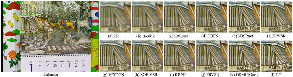
Figure 6: Qualitative results by different methods on the Vid4 dataset.

Table 3: Ablation studies on our DSMC. $Comm.$ is short for communication, and $MSCU_{(\cdot)}$ denotes the submodule of MSCU. The most effective module and the second one are in red boldface and blue boldface, respectively.

Ablation	PSNR/SSIM	$\Delta$
Bicubic	23.72/0.7559	-2.01/-0.0869
w/o MSCU	20.48/0.6264	-5.25/-0.2164
w/o MSCUResNet	24.81/0.8210	-0.92/-0.0218
w/o MSCUComm.	22.30/0.6853	-3.43/-0.1575
w/o MSCUResNet+Comm.	21.77/0.6711	-3.96/-0.1717
w/o U3D-RDN	22.64/0.7093	-3.09/-0.1335
w/o U3D-RDNNon_local	25.59/0.8378	-0.14/-0.0050
DSMC (Baseline)	25.73/0.8428	0.00/0.0000

Table 4: FLOPs and parameter numbers of traditional 3D-RDN (without U-shaped structure) and the proposed U3D-RDN. Note that the mini-batch size of the test data is 1.

Module	FLOPs	Params.
3D-RDN	509.17G	2.48M
U3D-RDN	129.18G	2.52M

Table 5: Ablation studies on the dual loss. $Perc.$ is short for perceptual loss. Noted that the best results are in red boldface and the second best results are in blue boldface.

Cb	Perc.	Dual Cb	Dual Perc.	PSNR/SSIM
$\checkmark$				25.70/0.8408
$\checkmark$		$\checkmark$		25.71/0.8420
$\checkmark$	$\checkmark$			25.67/0.8413
$\checkmark$	$\checkmark$	$\checkmark$	$\checkmark$	25.73/0.8428

Ablation studies

In order to verify the effectiveness of each module, we do several ablation studies on important modules of DSMC. We use video clips in the validation set of REDS for test. The experimental results are shown in Table 3. In details, we ablate the MSCU module by replacing it with a $\times 4$ upsampling layer, and the communication mechanism by simply executing two $\times 2$ upsampling.

It is seen that MSCU poses the most significant influence on the performance of DSMC, while the join of feature correction network (ResNet) and communication mechanism is the key factor that determines the ability of MSCU. Particularly, U3D-RDN also plays an important role, which indicates that it has strong ability for modeling large motion in videos. Furthermore, we do an extra study to demonstrate the effectiveness of U3D-RDN on reducing computational complexity, as shown in Table 4. Obviously, the proposed U3D-RDN has reduced 74.6% of the computational cost with only 0.04M additional parameters.

In addition, we also analyze the effectiveness of the dual subnet in Table 5. We train 4 models of DSMC with different loss functions. Among them, the Cb and perceptual loss functions are used for the VSR subnet, and the dual Cb and dual perceptual losses are for the dual subnet. The results show that when both the VSR subnet and the dual subnet use Cb and perceptual losses, the values of PSNR and SSIM are the best. It confirms the strict dual learning mechanism. Moreover, the second best performance is obtained when both the VSR and the dual subnet employ only Cb loss. Additionally, when there is no dual subnet (e.g. only Cb loss exists), the performance of DSMC degrades, which indicates the role of dual subnet. It is noted that the contribution brought by the dual subnet is less obvious than the proposed VSR subnet according to Tables 3 and 5, which demonstrate that a reasonable design of a VSR network is of more vital importance than an ingenious training strategy.

Conclusion

In this paper, we proposed a novel Video Super-Resolution Network with Dual Subnet and Multi-Stage Communicated Upsampling (DSMC). We designed a new U-shaped residual dense network with 3D convolution (U3D-RDN) for our DSMC, which can achieve both fine implicit motion estimation and motion compensation (MEMC) and coarse spatial feature extraction as well as reducing the computational complexity. Moreover, we proposed a Multi-Stage Communicated Upsampling (MSCU) module for helping utilize intermediate information during upsampling, and a dual subnet which can enhance the generalization ability. Extensive experimental results confirmed the effectiveness of our method in processing videos with large motion for $\times 4$ VSR tasks. Additionally, we did ablation studies on important modules of our DSMC. They indicated that U3D-RDN and MSCU are the key modules that affect the performance of DSMC. Meanwhile, the proposed dual loss can help DSMC converge to a better solution. We believe that our work can provide a better viewing experience for extreme sports fans and outdoor photographers. In the future, we will improve our design for large-scale video super-resolution.

References

- Caballero et al. (2017) Caballero, J.; Ledig, C.; Aitken, A.; Acosta, A.; Totz, J.; Wang, Z.; and Shi, W. 2017. Real-time video super-resolution with spatio-temporal networks and motion compensation. In Proceedings of the IEEE Conference on Computer Vision and Pattern Recognition, 4778–4787.
- Cui et al. (2019) Cui, Y.; Jia, M.; Lin, T.-Y.; Song, Y.; and Belongie, S. 2019. Class-balanced loss based on effective number of samples. In Proceedings of the IEEE Conference on Computer Vision and Pattern Recognition, 9268–9277.
- Dong et al. (2015) Dong, C.; Loy, C. C.; He, K.; and Tang, X. 2015. Image super-resolution using deep convolutional networks. IEEE Transactions on Pattern Analysis and Machine Intelligence 38(2): 295–307.
- Drulea and Nedevschi (2011) Drulea, M.; and Nedevschi, S. 2011. Total variation regularization of local-global optical flow. In 2011 14th International IEEE Conference on Intelligent Transportation Systems (ITSC), 318–323. IEEE.
- Gibson (1957) Gibson, J. J. 1957. Optical motions and transformations as stimuli for visual perception. Psychological Review 64(5): 288.
- Gu et al. (2019) Gu, J.; Lu, H.; Zuo, W.; and Dong, C. 2019. Blind super-resolution with iterative kernel correction. In Proceedings of the IEEE Conference on Computer Vision and Pattern Recognition, 1604–1613.
- Guo et al. (2020) Guo, Y.; Chen, J.; Wang, J.; Chen, Q.; Cao, J.; Deng, Z.; Xu, Y.; and Tan, M. 2020. Closed-loop Matters: Dual Regression Networks for Single Image Super-Resolution. arXiv Preprint arXiv:2003.07018 .
- Haris, Shakhnarovich, and Ukita (2018) Haris, M.; Shakhnarovich, G.; and Ukita, N. 2018. Deep back-projection networks for super-resolution. In Proceedings of the IEEE Conference on Computer Vision and Pattern Recognition, 1664–1673.
- Haris, Shakhnarovich, and Ukita (2019) Haris, M.; Shakhnarovich, G.; and Ukita, N. 2019. Recurrent back-projection network for video super-resolution. In Proceedings of the IEEE Conference on Computer Vision and Pattern Recognition, 3897–3906.
- He et al. (2016a) He, D.; Xia, Y.; Qin, T.; Wang, L.; Yu, N.; Liu, T.-Y.; and Ma, W.-Y. 2016a. Dual learning for machine translation. In Advances in Neural Information Processing Systems, 820–828.
- He et al. (2016b) He, K.; Zhang, X.; Ren, S.; and Sun, J. 2016b. Deep residual learning for image recognition. In Proceedings of the IEEE Conference on Computer Vision and Pattern Recognition, 770–778.
- Huang et al. (2017) Huang, G.; Liu, Z.; Van Der Maaten, L.; and Weinberger, K. Q. 2017. Densely connected convolutional networks. In Proceedings of the IEEE Conference on Computer Vision and Pattern Recognition, 4700–4708.
- Ilg et al. (2017) Ilg, E.; Mayer, N.; Saikia, T.; Keuper, M.; Dosovitskiy, A.; and Brox, T. 2017. Flownet 2.0: Evolution of optical flow estimation with deep networks. In Proceedings of the IEEE Conference on Computer Vision and Pattern Recognition, 2462–2470.
- Jaderberg et al. (2015) Jaderberg, M.; Simonyan, K.; Zisserman, A.; et al. 2015. Spatial transformer networks. In Advances in Neural Information Processing Systems, 2017–2025.
- Ji et al. (2012) Ji, S.; Xu, W.; Yang, M.; and Yu, K. 2012. 3D convolutional neural networks for human action recognition. IEEE Transactions on Pattern Analysis and Machine Intelligence 35(1): 221–231.
- Jia et al. (2016) Jia, X.; De Brabandere, B.; Tuytelaars, T.; and Gool, L. V. 2016. Dynamic filter networks. In Advances in Neural Information Processing Systems, 667–675.
- Jo et al. (2018) Jo, Y.; Wug Oh, S.; Kang, J.; and Joo Kim, S. 2018. Deep video super-resolution network using dynamic upsampling filters without explicit motion compensation. In Proceedings of the IEEE Conference on Computer Vision and Pattern Recognition, 3224–3232.
- Johnson, Alahi, and Li (2016) Johnson, J.; Alahi, A.; and Li, F.-F. 2016. Perceptual losses for real-time style transfer and super-resolution. In European Conference on Computer Vision, 694–711. Springer.
- Kalarot and Porikli (2019) Kalarot, R.; and Porikli, F. 2019. MultiBoot VSR: Multi-Stage Multi-Reference Bootstrapping for Video Super-Resolution. In Proceedings of the IEEE Conference on Computer Vision and Pattern Recognition Workshops, 0–0.
- Kappeler et al. (2016) Kappeler, A.; Yoo, S.; Dai, Q.; and Katsaggelos, A. K. 2016. Video super-resolution with convolutional neural networks. IEEE Transactions on Computational Imaging 2(2): 109–122.
- Kim, Kwon Lee, and Mu Lee (2016) Kim, J.; Kwon Lee, J.; and Mu Lee, K. 2016. Accurate image super-resolution using very deep convolutional networks. In Proceedings of the IEEE Conference on Computer Vision and Pattern Recognition, 1646–1654.
- Kim et al. (2018) Kim, S. Y.; Lim, J.; Na, T.; and Kim, M. 2018. 3DSRnet: Video Super-resolution using 3D Convolutional Neural Networks. arXiv Preprint arXiv:1812.09079 .
- Lei and Todorovic (2018) Lei, P.; and Todorovic, S. 2018. Temporal deformable residual networks for action segmentation in videos. In Proceedings of the IEEE Conference on Computer Vision and Pattern Recognition, 6742–6751.
- Li et al. (2019) Li, S.; He, F.; Du, B.; Zhang, L.; Xu, Y.; and Tao, D. 2019. Fast spatio-temporal residual network for video super-resolution. In Proceedings of the IEEE Conference on Computer Vision and Pattern Recognition, 10522–10531.
- Liao et al. (2015) Liao, R.; Tao, X.; Li, R.; Ma, Z.; and Jia, J. 2015. Video super-resolution via deep draft-ensemble learning. In Proceedings of the IEEE International Conference on Computer Vision, 531–539.
- Lim et al. (2017) Lim, B.; Son, S.; Kim, H.; Nah, S.; and Mu Lee, K. 2017. Enhanced deep residual networks for single image super-resolution. In Proceedings of the IEEE Conference on Computer Vision and Pattern Recognition Workshops, 136–144.
- Liu et al. (2020a) Liu, H.; Ruan, Z.; Fang, C.; Zhao, P.; Shang, F.; Liu, Y.; and Wang, L. 2020a. A Single Frame and Multi-Frame Joint Network for 360-degree Panorama Video Super-Resolution. arXiv Preprint arXiv:2008.10320 .
- Liu et al. (2020b) Liu, H.; Ruan, Z.; Zhao, P.; Shang, F.; Yang, L.; and Liu, Y. 2020b. Video Super Resolution Based on Deep Learning: A comprehensive survey. arXiv Preprint arXiv:2007.12928 .
- Mnih et al. (2014) Mnih, V.; Heess, N.; Graves, A.; et al. 2014. Recurrent models of visual attention. In Advances in Neural Information Processing Systems, 2204–2212.
- Nah et al. (2019) Nah, S.; Baik, S.; Hong, S.; Moon, G.; Son, S.; Timofte, R.; and Lee, K. M. 2019. NTIRE 2019 Challenge on Video Deblurring and Super-Resolution: Dataset and Study. In The IEEE Conference on Computer Vision and Pattern Recognition (CVPR) Workshops.
- Ranjan and Black (2017) Ranjan, A.; and Black, M. J. 2017. Optical flow estimation using a spatial pyramid network. In Proceedings of the IEEE Conference on Computer Vision and Pattern Recognition, 4161–4170.
- Sajjadi, Vemulapalli, and Brown (2018) Sajjadi, M. S.; Vemulapalli, R.; and Brown, M. 2018. Frame-recurrent video super-resolution. In Proceedings of the IEEE Conference on Computer Vision and Pattern Recognition, 6626–6634.
- Shi et al. (2016) Shi, W.; Caballero, J.; Huszár, F.; Totz, J.; Aitken, A. P.; Bishop, R.; Rueckert, D.; and Wang, Z. 2016. Real-time single image and video super-resolution using an efficient sub-pixel convolutional neural network. In Proceedings of the IEEE Conference on Computer Vision and Pattern Recognition, 1874–1883.
- Simonyan and Zisserman (2014) Simonyan, K.; and Zisserman, A. 2014. Very deep convolutional networks for large-scale image recognition. arXiv Preprint arXiv:1409.1556 .
- Tao et al. (2017) Tao, X.; Gao, H.; Liao, R.; Wang, J.; and Jia, J. 2017. Detail-revealing deep video super-resolution. In Proceedings of the IEEE International Conference on Computer Vision, 4472–4480.
- Tian et al. (2020) Tian, Y.; Zhang, Y.; Fu, Y.; and Xu, C. 2020. TDAN: Temporally-Deformable Alignment Network for Video Super-Resolution. In Proceedings of the IEEE Conference on Computer Vision and Pattern Recognition, 3360–3369.
- Wang et al. (2018a) Wang, L.; Guo, Y.; Lin, Z.; Deng, X.; and An, W. 2018a. Learning for video super-resolution through HR optical flow estimation. In Asian Conference on Computer Vision, 514–529. Springer.
- Wang et al. (2018b) Wang, X.; Girshick, R.; Gupta, A.; and He, K. 2018b. Non-local neural networks. In Proceedings of the IEEE Conference on Computer Vision and Pattern Recognition, 7794–7803.
- Xin et al. (2020) Xin, J.; Wang, N.; Li, J.; Gao, X.; and Li, Z. 2020. Video Face Super-Resolution with Motion-Adaptive Feedback Cell. In AAAI, 12468–12475.
- Xue et al. (2019) Xue, T.; Chen, B.; Wu, J.; Wei, D.; and Freeman, W. T. 2019. Video enhancement with task-oriented flow. International Journal of Computer Vision 127(8): 1106–1125.
- Ying et al. (2020) Ying, X.; Wang, L.; Wang, Y.; Sheng, W.; An, W.; and Guo, Y. 2020. Deformable 3D Convolution for Video Super-Resolution. arXiv Preprint arXiv:2004.02803 .
- Zhang et al. (2018a) Zhang, Y.; Li, K.; Li, K.; Wang, L.; Zhong, B.; and Fu, Y. 2018a. Image super-resolution using very deep residual channel attention networks. In Proceedings of the European Conference on Computer Vision (ECCV), 286–301.
- Zhang et al. (2018b) Zhang, Y.; Tian, Y.; Kong, Y.; Zhong, B.; and Fu, Y. 2018b. Residual dense network for image super-resolution. In Proceedings of the IEEE Conference on Computer Vision and Pattern Recognition, 2472–2481.