Abstract
We derive a simple and precise approximation to probability density functions in sampling distributions based on the Fourier cosine series.
After clarifying the required conditions, we illustrate the approximation on two examples: the distribution of the sum of uniformly distributed random variables, and
the distribution of sample skewness drawn from a normal population.
The probability density function of the first example can be explicitly expressed, but that of the second example has no explicit expression.
1 Introduction
Fourier series and their transforms are widely applied in statistics because they are mathematically tractable. For instance, they are uniformly convergent within a closed interval and can be integrated
term by term (Whittaker [10 ] ).
Substantial applications are
the generalized representations (or estimations) of statistical curves such as
probability density functions (pdfs) and their associated cumulative distribution functions (cdfs).
(see, for example, Kronmal and Tarter [5 ] ).
Many approximations to pdfs or cdfs have been developed in sampling distribution theory.
The Edgeworth series of the pdf of a statistic, a well-known series that
refines the central limit theorem, is composed of Hermite polynomials as orthogonal polynomials.
Meanwhile, the Fourier series are composed of orthogonal trigonometric functions and their approximation target slightly differs from that of the Edgeworth series.
Whereas the Edgeworth series handles cases with bounded of unbounded pdf support,
the Fourier series requires a bounded support and a periodic pdf.
It appears that the Fourier coefficients must be obtained under severe constraints.
In this paper, we approximate the pdf or cdf using cosine Fourier series, and
provide three conditions that must be satisfied.
First, the pdf requires a bounded support.
Second, the function must be piecewise smooth and even.
Finally, the pdf must have moments up to the required order.
We remark that the first and second conditions are technical only, but the third is crucial.
We also remark that sampling distributions are evaluated by numerous statistics, for example,
sample skewness, sample kurtosis, the Shapiro–Wilk test statistic, and sample correlation coefficient.
The remainder of this paper is organized as follows.
Section 2 3 4 3 4 b 1 absent subscript 𝑏 1 \sqrt{\vrule width=0.0pt,height=5.16663pt}{b_{1}} n = 3 𝑛 3 n=3 4 4 4 [3 ] and McKay [6 ] , respectively; for other sample sizes, they are unknown.
Here, we mention the sample of size n 𝑛 n n 𝑛 n b 1 absent subscript 𝑏 1 \sqrt{\vrule width=0.0pt,height=5.16663pt}{b_{1}} n / 6 𝑛 6 n/6 [9 ] ).
When n 𝑛 n [1 ] transformation works well.
When n 𝑛 n [7 ] approximations are valid,
but the mathematical expressions of the pdfs are very complicated.
Based on the Fourier cosine series,
we provide concrete approximations of the sampling distribution, which are particularly effective when n 𝑛 n b 1 absent subscript 𝑏 1 \sqrt{\vrule width=0.0pt,height=5.16663pt}{b_{1}}
2 Fourier series of probability density functions
Let T n = T n ( X 1 , X 2 , … , X n ) subscript 𝑇 𝑛 subscript 𝑇 𝑛 subscript 𝑋 1 subscript 𝑋 2 … subscript 𝑋 𝑛 \displaystyle T_{n}=T_{n}\left(X_{1},X_{2},\ldots,X_{n}\right) f n ( x ) subscript 𝑓 𝑛 𝑥 f_{n}(x) ( X 1 , X 2 , … , X n ) subscript 𝑋 1 subscript 𝑋 2 … subscript 𝑋 𝑛 \left(\displaystyle X_{1},X_{2},\ldots,X_{n}\right) n 𝑛 n
1.
f n ( x ) subscript 𝑓 𝑛 𝑥 f_{n}(x) [ − A n , A n ] subscript 𝐴 𝑛 subscript 𝐴 𝑛 [-A_{n},A_{n}] A n > 0 subscript 𝐴 𝑛 0 A_{n}>0
2.
f n ( x ) subscript 𝑓 𝑛 𝑥 f_{n}(x)
From Condition 1 and 2,
f n ( x ) subscript 𝑓 𝑛 𝑥 f_{n}(x) [ − A n , A n ] subscript 𝐴 𝑛 subscript 𝐴 𝑛 [-A_{n},A_{n}]
f n ( x ) = a n , 0 2 + ∑ k = 1 ∞ a n , k cos k π A n x , subscript 𝑓 𝑛 𝑥 subscript 𝑎 𝑛 0
2 superscript subscript 𝑘 1 subscript 𝑎 𝑛 𝑘
𝑘 𝜋 subscript 𝐴 𝑛 𝑥 f_{n}(x)=\frac{a_{n,0}}{2}+\sum_{k=1}^{\infty}a_{n,k}\cos\frac{k\pi}{A_{n}}x, (1)
where
the Fourier cosine coefficients a n , k subscript 𝑎 𝑛 𝑘
a_{n,k}
a n , 0 subscript 𝑎 𝑛 0
\displaystyle a_{n,0} = 1 A n ∫ − A n A n f n ( x ) 𝑑 x = 1 A n , absent 1 subscript 𝐴 𝑛 superscript subscript subscript 𝐴 𝑛 subscript 𝐴 𝑛 subscript 𝑓 𝑛 𝑥 differential-d 𝑥 1 subscript 𝐴 𝑛 \displaystyle=\frac{1}{A_{n}}\int_{-A_{n}}^{A_{n}}f_{n}(x)\,dx=\frac{1}{A_{n}},
a n , k subscript 𝑎 𝑛 𝑘
\displaystyle a_{n,k} = 1 A n ∫ − A n A n f n ( x ) cos k π A n x d x . absent 1 subscript 𝐴 𝑛 superscript subscript subscript 𝐴 𝑛 subscript 𝐴 𝑛 subscript 𝑓 𝑛 𝑥 𝑘 𝜋 subscript 𝐴 𝑛 𝑥 𝑑 𝑥 \displaystyle=\frac{1}{A_{n}}\int_{-A_{n}}^{A_{n}}f_{n}(x)\cos\frac{k\pi}{A_{n}}x\,dx. (2)
We also assume that the moments of T n subscript 𝑇 𝑛 T_{n}
3.
For any j 𝑗 j μ n , j ′ = ∫ − ∞ ∞ x j f n ( x ) 𝑑 x < ∞ superscript subscript 𝜇 𝑛 𝑗
′ superscript subscript superscript 𝑥 𝑗 subscript 𝑓 𝑛 𝑥 differential-d 𝑥 \mu_{n,j}^{\prime}=\displaystyle\int_{-\infty}^{\infty}x^{j}f_{n}(x)\,dx<\infty
From Condition 3 and
cos x = ∑ j = 0 ∞ ( − 1 ) j ( 2 j ) ! x 2 j 𝑥 superscript subscript 𝑗 0 superscript 1 𝑗 2 𝑗 superscript 𝑥 2 𝑗 \displaystyle\cos x=\sum_{j=0}^{\infty}\frac{(-1)^{j}}{(2j)!}x^{2j} a n , k subscript 𝑎 𝑛 𝑘
a_{n,k}
a n , k subscript 𝑎 𝑛 𝑘
\displaystyle a_{n,k} = 1 A n ∫ − A n A n f n ( x ) ∑ j = 0 ∞ ( − 1 ) j ( 2 j ) ! ( k π A n ) 2 j x 2 j d x absent 1 subscript 𝐴 𝑛 superscript subscript subscript 𝐴 𝑛 subscript 𝐴 𝑛 subscript 𝑓 𝑛 𝑥 superscript subscript 𝑗 0 superscript 1 𝑗 2 𝑗 superscript 𝑘 𝜋 subscript 𝐴 𝑛 2 𝑗 superscript 𝑥 2 𝑗 𝑑 𝑥 \displaystyle=\frac{1}{A_{n}}\int_{-A_{n}}^{A_{n}}f_{n}(x)\sum_{j=0}^{\infty}\frac{(-1)^{j}}{(2j)!}\left(\frac{k\pi}{A_{n}}\right)^{2j}x^{2j}\,dx
= 1 A n ∑ j = 0 ∞ ( − 1 ) j ( 2 j ) ! ( k π A n ) 2 j μ n , 2 j ′ , absent 1 subscript 𝐴 𝑛 superscript subscript 𝑗 0 superscript 1 𝑗 2 𝑗 superscript 𝑘 𝜋 subscript 𝐴 𝑛 2 𝑗 superscript subscript 𝜇 𝑛 2 𝑗
′ \displaystyle=\frac{1}{A_{n}}\sum_{j=0}^{\infty}\frac{(-1)^{j}}{(2j)!}\left(\frac{k\pi}{A_{n}}\right)^{2j}\mu_{n,2j}^{\prime}, (3)
where we have performed termwise integration.
The cumulative distribution function F n ( x ) = Pr { T n < x } subscript 𝐹 𝑛 𝑥 Pr subscript 𝑇 𝑛 𝑥 F_{n}(x)=\Pr\left\{T_{n}<x\right\}
F n ( x ) = 1 2 ( x A n + 1 ) + ∑ k = 1 ∞ a n , k A n k π sin k π A n x . subscript 𝐹 𝑛 𝑥 1 2 𝑥 subscript 𝐴 𝑛 1 superscript subscript 𝑘 1 subscript 𝑎 𝑛 𝑘
subscript 𝐴 𝑛 𝑘 𝜋 𝑘 𝜋 subscript 𝐴 𝑛 𝑥 F_{n}(x)=\frac{1}{2}\left(\frac{x}{A_{n}}+1\right)+\sum_{k=1}^{\infty}\frac{a_{n,k}A_{n}}{k\pi}\sin\frac{k\pi}{A_{n}}x.
From the Fourier cosine series (1 f n ( x ) subscript 𝑓 𝑛 𝑥 f_{n}(x)
f n ~ ( K ) ( x ) = a n , 0 2 + ∑ k = 1 K a n , k cos k π A n x superscript ~ subscript 𝑓 𝑛 𝐾 𝑥 subscript 𝑎 𝑛 0
2 superscript subscript 𝑘 1 𝐾 subscript 𝑎 𝑛 𝑘
𝑘 𝜋 subscript 𝐴 𝑛 𝑥 \widetilde{f_{n}}^{(K)}(x)=\frac{a_{n,0}}{2}+\sum_{k=1}^{K}a_{n,k}\cos\frac{k\pi}{A_{n}}x (4)
and
F n ~ ( K ) ( x ) = 1 2 ( x A n + 1 ) + ∑ k = 1 K a n , k A n k π sin k π A n x superscript ~ subscript 𝐹 𝑛 𝐾 𝑥 1 2 𝑥 subscript 𝐴 𝑛 1 superscript subscript 𝑘 1 𝐾 subscript 𝑎 𝑛 𝑘
subscript 𝐴 𝑛 𝑘 𝜋 𝑘 𝜋 subscript 𝐴 𝑛 𝑥 \widetilde{F_{n}}^{(K)}(x)=\frac{1}{2}\left(\frac{x}{A_{n}}+1\right)+\sum_{k=1}^{K}\frac{a_{n,k}A_{n}}{k\pi}\sin\frac{k\pi}{A_{n}}x (5)
are the best approximations because they minimize
∫ − A n A n ( f n ~ ( K ) ( x ) − f n ( x ) ) 2 𝑑 x and ∫ − A n A n ( F n ~ ( K ) ( x ) − F n ( x ) ) 2 𝑑 x , superscript subscript subscript 𝐴 𝑛 subscript 𝐴 𝑛 superscript superscript ~ subscript 𝑓 𝑛 𝐾 𝑥 subscript 𝑓 𝑛 𝑥 2 differential-d 𝑥 and superscript subscript subscript 𝐴 𝑛 subscript 𝐴 𝑛 superscript superscript ~ subscript 𝐹 𝑛 𝐾 𝑥 subscript 𝐹 𝑛 𝑥 2 differential-d 𝑥
\displaystyle\int_{-A_{n}}^{A_{n}}\left(\widetilde{f_{n}}^{(K)}(x)-f_{n}(x)\right)^{2}\,dx\qquad\mbox{and}\qquad\displaystyle\int_{-A_{n}}^{A_{n}}\left(\widetilde{F_{n}}^{(K)}(x)-F_{n}(x)\right)^{2}\,dx,
respectively (Whittaker [10 ] ).
•
Solving the nonlinear equation F n ~ ( K ) ( x ) = α superscript ~ subscript 𝐹 𝑛 𝐾 𝑥 𝛼 \widetilde{F_{n}}^{(K)}(x)=\alpha x 0.5 = 0 subscript 𝑥 0.5 0 x_{0.5}=0 x α ( 0 < α < 1 ) subscript 𝑥 𝛼 0 𝛼 1 x_{\alpha}\,(0<\alpha<1)
•
If f n ( x ) subscript 𝑓 𝑛 𝑥 f_{n}(x) a n , k subscript 𝑎 𝑛 𝑘
a_{n,k} 2 f n ( x ) subscript 𝑓 𝑛 𝑥 f_{n}(x) μ n , j ′ superscript subscript 𝜇 𝑛 𝑗
′ \mu_{n,j}^{\prime} 4 3
We approximate the Fourier cosine coefficients (2
a n , k ^ ( J ) = 1 A n ∑ j = 0 J ( − 1 ) j ( 2 j ) ! ( k π A n ) 2 j μ n , 2 j ′ superscript ^ subscript 𝑎 𝑛 𝑘
𝐽 1 subscript 𝐴 𝑛 superscript subscript 𝑗 0 𝐽 superscript 1 𝑗 2 𝑗 superscript 𝑘 𝜋 subscript 𝐴 𝑛 2 𝑗 superscript subscript 𝜇 𝑛 2 𝑗
′ \widehat{a_{n,k}}^{(J)}=\frac{1}{A_{n}}\sum_{j=0}^{J}\frac{(-1)^{j}}{(2j)!}\left(\frac{k\pi}{A_{n}}\right)^{2j}\mu_{n,2j}^{\prime}
and Eqs. (4 5
f n ^ ( K , J ) ( x ) superscript ^ subscript 𝑓 𝑛 𝐾 𝐽 𝑥 \displaystyle\widehat{f_{n}}^{(K,J)}(x) = a n , 0 2 + ∑ k = 1 K a n , k ^ ( J ) cos k π A n x , absent subscript 𝑎 𝑛 0
2 superscript subscript 𝑘 1 𝐾 superscript ^ subscript 𝑎 𝑛 𝑘
𝐽 𝑘 𝜋 subscript 𝐴 𝑛 𝑥 \displaystyle=\frac{a_{n,0}}{2}+\sum_{k=1}^{K}\widehat{a_{n,k}}^{(J)}\cos\frac{k\pi}{A_{n}}x,
F n ^ ( K , J ) ( x ) superscript ^ subscript 𝐹 𝑛 𝐾 𝐽 𝑥 \displaystyle\widehat{F_{n}}^{(K,J)}(x) = 1 2 ( x A n + 1 ) + ∑ k = 1 K a n , k ^ ( J ) A n k π sin k π A n x , absent 1 2 𝑥 subscript 𝐴 𝑛 1 superscript subscript 𝑘 1 𝐾 superscript ^ subscript 𝑎 𝑛 𝑘
𝐽 subscript 𝐴 𝑛 𝑘 𝜋 𝑘 𝜋 subscript 𝐴 𝑛 𝑥 \displaystyle=\frac{1}{2}\left(\frac{x}{A_{n}}+1\right)+\sum_{k=1}^{K}\frac{\widehat{a_{n,k}}^{(J)}A_{n}}{k\pi}\sin\frac{k\pi}{A_{n}}x,
respectively.
Note that the choices of K 𝐾 K J 𝐽 J n 𝑛 n
3 Distribution of a sum of random variabels uniformly distributed
Random variables X 1 , X 2 , … , X n subscript 𝑋 1 subscript 𝑋 2 … subscript 𝑋 𝑛
X_{1},X_{2},\ldots,X_{n} [ − 1 2 , 1 2 ] 1 2 1 2 \displaystyle\left[-\frac{1}{2},\,\frac{1}{2}\right] f n ( x ) subscript 𝑓 𝑛 𝑥 f_{n}(x) T n = X 1 + X 2 + ⋯ + X n subscript 𝑇 𝑛 subscript 𝑋 1 subscript 𝑋 2 ⋯ subscript 𝑋 𝑛 T_{n}=X_{1}+X_{2}+\cdots+X_{n}
f n ( x ) = ∫ − ∞ ∞ f n − 1 ( x − t ) f 1 ( t ) 𝑑 t = ∫ x − 1 / 2 x + 1 / 2 f n − 1 ( t ) 𝑑 t ( n ≥ 2 ) , formulae-sequence subscript 𝑓 𝑛 𝑥 superscript subscript subscript 𝑓 𝑛 1 𝑥 𝑡 subscript 𝑓 1 𝑡 differential-d 𝑡 superscript subscript 𝑥 1 2 𝑥 1 2 subscript 𝑓 𝑛 1 𝑡 differential-d 𝑡 𝑛 2 f_{n}(x)=\int_{-\infty}^{\infty}f_{n-1}(x-t)f_{1}(t)\,dt=\int_{x-1/2}^{x+1/2}f_{n-1}(t)\,dt\qquad(n\geq 2),
f 1 ( x ) = { 1 ( − 1 2 ≤ x ≤ 1 2 ) 0 ( otherwise ) , subscript 𝑓 1 𝑥 cases 1 1 2 𝑥 1 2 0 otherwise f_{1}(x)=\begin{cases}1&\left(-\frac{1}{2}\leq x\leq\frac{1}{2}\right)\\
0&(\rm{otherwise}),\end{cases}
for any
− n 2 + i ≤ x ≤ − n 2 + i + 1 ( i = 0 , 1 , … , n − 1 ) 𝑛 2 𝑖 𝑥 𝑛 2 𝑖 1 𝑖 0 1 … 𝑛 1
\displaystyle-\frac{n}{2}+i\leq x\leq-\frac{n}{2}+i+1\,(i=0,1,\ldots,n-1)
f n ( x ) = 1 ( n − 1 ) ! ∑ j = 0 i ( − 1 ) j ( n j ) ( x + n 2 − j ) n − 1 , subscript 𝑓 𝑛 𝑥 1 𝑛 1 superscript subscript 𝑗 0 𝑖 superscript 1 𝑗 binomial 𝑛 𝑗 superscript 𝑥 𝑛 2 𝑗 𝑛 1 f_{n}(x)=\frac{1}{(n-1)!}\sum_{j=0}^{i}(-1)^{j}{n\choose j}\left(x+\frac{n}{2}-j\right)^{n-1},
f n ( x ) = 0 ( otherwise ) subscript 𝑓 𝑛 𝑥 0 otherwise f_{n}(x)=0\,(\mbox{otherwise}) f n ( x ) subscript 𝑓 𝑛 𝑥 f_{n}(x) [ − n 2 , n 2 ] 𝑛 2 𝑛 2 \displaystyle\left[-\frac{n}{2},\frac{n}{2}\right] μ n , j ′ superscript subscript 𝜇 𝑛 𝑗
′ \mu_{n,j}^{\prime}
μ n , 2 j ′ = ∑ k = 0 j ( 2 j 2 k ) 1 ( 2 k + 1 ) 4 k μ n − 1 , 2 j − 2 k ′ . superscript subscript 𝜇 𝑛 2 𝑗
′ superscript subscript 𝑘 0 𝑗 binomial 2 𝑗 2 𝑘 1 2 𝑘 1 superscript 4 𝑘 superscript subscript 𝜇 𝑛 1 2 𝑗 2 𝑘
′ \mu_{n,2j}^{\prime}=\sum_{k=0}^{j}{2j\choose 2k}\frac{1}{(2k+1)4^{k}}\mu_{n-1,2j-2k}^{\prime}.
Example
When n = 4 𝑛 4 n=4
f 4 ( x ) = { 1 6 ( x + 2 ) 3 ( − 2 ≤ x ≤ − 1 ) 1 6 { ( x + 2 ) 3 − 4 ( x + 1 ) 3 } ( − 1 ≤ x ≤ 0 ) 1 6 { ( x + 2 ) 3 − 4 ( x + 1 ) 3 + 6 x 3 } ( 0 ≤ x ≤ 1 ) 1 6 { ( x + 2 ) 3 − 4 ( x + 1 ) 3 + 6 x 3 − 4 ( x − 1 ) 3 } ( 1 ≤ x ≤ 2 ) 0 ( otherwise ) . subscript 𝑓 4 𝑥 cases 1 6 superscript 𝑥 2 3 2 𝑥 1 1 6 superscript 𝑥 2 3 4 superscript 𝑥 1 3 1 𝑥 0 1 6 superscript 𝑥 2 3 4 superscript 𝑥 1 3 6 superscript 𝑥 3 0 𝑥 1 1 6 superscript 𝑥 2 3 4 superscript 𝑥 1 3 6 superscript 𝑥 3 4 superscript 𝑥 1 3 1 𝑥 2 0 otherwise f_{4}(x)=\begin{cases}\frac{1}{6}\left(x+2\right)^{3}&\left(-2\leq x\leq-1\right)\\
\frac{1}{6}\left\{\left(x+2\right)^{3}-4\left(x+1\right)^{3}\right\}&\left(-1\leq x\leq 0\right)\\
\frac{1}{6}\left\{\left(x+2\right)^{3}-4\left(x+1\right)^{3}+6x^{3}\right\}&\left(0\leq x\leq 1\right)\\
\frac{1}{6}\left\{\left(x+2\right)^{3}-4\left(x+1\right)^{3}+6x^{3}-4\left(x-1\right)^{3}\right\}&\left(1\leq x\leq 2\right)\\
0&(\mbox{otherwise}).\end{cases}
The even moments are given by
μ 4 , 2 j ′ = 8 ( 4 ⋅ 4 j − 1 ) ( 1 + 2 j ) ( 2 + 2 j ) ( 3 + 2 j ) ( 4 + 2 j ) , superscript subscript 𝜇 4 2 𝑗
′ 8 ⋅ 4 superscript 4 𝑗 1 1 2 𝑗 2 2 𝑗 3 2 𝑗 4 2 𝑗 \displaystyle\mu_{4,2j}^{\prime}=\frac{8\left(4\cdot 4^{j}-1\right)}{(1+2j)(2+2j)(3+2j)(4+2j)},
and
odd moments are all 0 0
The Fourier cosine series of f 4 ( x ) subscript 𝑓 4 𝑥 f_{4}(x) [ − 2 , 2 ] 2 2 [-2,2]
f 4 ( x ) = 1 4 + ∑ k = 1 ∞ a 4 , k cos k π 2 x , subscript 𝑓 4 𝑥 1 4 superscript subscript 𝑘 1 subscript 𝑎 4 𝑘
𝑘 𝜋 2 𝑥 f_{4}(x)=\frac{1}{4}+\sum_{k=1}^{\infty}a_{4,k}\cos\frac{k\pi}{2}x,
with coefficients
a 4 , k = 128 π 4 k 4 sin 4 ( k π 4 ) . subscript 𝑎 4 𝑘
128 superscript 𝜋 4 superscript 𝑘 4 superscript 4 𝑘 𝜋 4 a_{4,k}=\frac{128}{\pi^{4}k^{4}}\sin^{4}\left(\frac{k\pi}{4}\right).
The cumulative distribution function is
F 4 ( x ) = 1 2 + x 4 + ∑ k = 1 ∞ 2 a n , k k π sin k π 2 x . subscript 𝐹 4 𝑥 1 2 𝑥 4 superscript subscript 𝑘 1 2 subscript 𝑎 𝑛 𝑘
𝑘 𝜋 𝑘 𝜋 2 𝑥 F_{4}(x)=\frac{1}{2}+\frac{x}{4}+\sum_{k=1}^{\infty}\frac{2a_{n,k}}{k\pi}\sin\frac{k\pi}{2}x.
Table 1
max 0 ≤ k ≤ K | a n , k ( J ) − a n , k | subscript 0 𝑘 𝐾 superscript subscript 𝑎 𝑛 𝑘
𝐽 subscript 𝑎 𝑛 𝑘
\displaystyle\max_{0\leq k\leq K}\left|a_{n,k}^{(J)}-a_{n,k}\right|
values for n = 2 ( 2 ) 12 𝑛 2 2 12 n=2(2)12 a n , k ( J ) superscript subscript 𝑎 𝑛 𝑘
𝐽 a_{n,k}^{(J)} a n , k subscript 𝑎 𝑛 𝑘
a_{n,k}
Tables 2 3
f 4 ^ ( 8 , 35 ) ( x ) = superscript ^ subscript 𝑓 4 8 35 𝑥 absent \displaystyle\widehat{f_{4}}^{(8,35)}(x)\,= 2.5 × 10 − 1 + ( 3.28511 × 10 − 1 ) cos ( π x 2 ) + ( 8.21279 × 10 − 2 ) cos ( π x ) 2.5 superscript 10 1 3.28511 superscript 10 1 𝜋 𝑥 2 8.21279 superscript 10 2 𝜋 𝑥 \displaystyle\,\,2.5\times 10^{-1}+\left(3.28511\times 10^{-1}\right)\cos\left(\frac{\pi x}{2}\right)+\left(8.21279\times 10^{-2}\right)\cos(\pi x)
+ ( 4.0557 × 10 − 3 ) cos ( 3 π x 2 ) + ( 1.0306 × 10 − 14 ) cos ( 2 π x ) 4.0557 superscript 10 3 3 𝜋 𝑥 2 1.0306 superscript 10 14 2 𝜋 𝑥 \displaystyle+\left(4.0557\times 10^{-3}\right)\cos\left(\frac{3\pi x}{2}\right)+\left(1.0306\times 10^{-14}\right)\cos(2\pi x)
+ ( 5.25618 × 10 − 4 ) cos ( 5 π x 2 ) + ( 1.01392 × 10 − 3 ) cos ( 3 π x ) 5.25618 superscript 10 4 5 𝜋 𝑥 2 1.01392 superscript 10 3 3 𝜋 𝑥 \displaystyle+\left(5.25618\times 10^{-4}\right)\cos\left(\frac{5\pi x}{2}\right)+\left(1.01392\times 10^{-3}\right)\cos(3\pi x)
+ ( 1.36823 × 10 − 4 ) cos ( 7 π x 2 ) − ( 5.73436 × 10 − 10 ) cos ( 4 π x ) 1.36823 superscript 10 4 7 𝜋 𝑥 2 5.73436 superscript 10 10 4 𝜋 𝑥 \displaystyle+\left(1.36823\times 10^{-4}\right)\cos\left(\frac{7\pi x}{2}\right)-\left(5.73436\times 10^{-10}\right)\cos(4\pi x)
and
F 4 ^ ( 8 , 35 ) ( x ) = superscript ^ subscript 𝐹 4 8 35 𝑥 absent \displaystyle\widehat{F_{4}}^{(8,35)}(x)\,= 1 2 ( u 2 + 1 ) + ( 2.09137 × 10 − 1 ) sin ( π x 2 ) + ( 2.61421 × 10 − 2 ) sin ( π x ) 1 2 𝑢 2 1 2.09137 superscript 10 1 𝜋 𝑥 2 2.61421 superscript 10 2 𝜋 𝑥 \displaystyle\,\,\frac{1}{2}\left(\frac{u}{2}+1\right)+\left(2.09137\times 10^{-1}\right)\sin\left(\frac{\pi x}{2}\right)+\left(2.61421\times 10^{-2}\right)\sin(\pi x)
+ ( 8.60646 × 10 − 4 ) sin ( 3 π x 2 ) + ( 1.64026 × 10 − 15 ) sin ( 2 π x ) 8.60646 superscript 10 4 3 𝜋 𝑥 2 1.64026 superscript 10 15 2 𝜋 𝑥 \displaystyle+\left(8.60646\times 10^{-4}\right)\sin\left(\frac{3\pi x}{2}\right)+\left(1.64026\times 10^{-15}\right)\sin(2\pi x)
+ ( 6.69238 × 10 − 5 ) sin ( 5 π x 2 ) + ( 1.07581 × 10 − 4 ) sin ( 3 π x ) 6.69238 superscript 10 5 5 𝜋 𝑥 2 1.07581 superscript 10 4 3 𝜋 𝑥 \displaystyle+\left(6.69238\times 10^{-5}\right)\sin\left(\frac{5\pi x}{2}\right)+\left(1.07581\times 10^{-4}\right)\sin(3\pi x)
+ ( 1.24434 × 10 − 5 ) sin ( 7 π x 2 ) − ( 4.56326 × 10 − 11 ) sin ( 4 π x ) . 1.24434 superscript 10 5 7 𝜋 𝑥 2 4.56326 superscript 10 11 4 𝜋 𝑥 \displaystyle+\left(1.24434\times 10^{-5}\right)\sin\left(\frac{7\pi x}{2}\right)-\left(4.56326\times 10^{-11}\right)\sin(4\pi x).
Table 4 x α subscript 𝑥 𝛼 x_{\alpha} T n subscript 𝑇 𝑛 T_{n} α 𝛼 \alpha n = 4 𝑛 4 n=4 α = 0.99 𝛼 0.99 \alpha=0.99
F 4 ^ ( 8 , 35 ) ( x ) = 0.99 superscript ^ subscript 𝐹 4 8 35 𝑥 0.99 \widehat{F_{4}}^{(8,35)}(x)=0.99
gives x 0.99 = 1.3002 subscript 𝑥 0.99 1.3002 x_{0.99}=1.3002
∫ − 2 x 0.99 f 4 ( x ) 𝑑 x = 0.990006 . superscript subscript 2 subscript 𝑥 0.99 subscript 𝑓 4 𝑥 differential-d 𝑥 0.990006 \int_{-2}^{x_{0.99}}f_{4}(x)\,dx=0.990006.
Table 1: Values of max 0 ≤ k ≤ K | a n , k ( J ) − a n , k | subscript 0 𝑘 𝐾 superscript subscript 𝑎 𝑛 𝑘
𝐽 subscript 𝑎 𝑛 𝑘
\displaystyle\max_{0\leq k\leq K}\left|a_{n,k}^{(J)}-a_{n,k}\right| n 𝑛 n K 𝐾 K J 𝐽 J
Table 2: Fourier coefficients a ^ 2 , k ( 35 ) , a ^ 4 , k ( 35 ) , a ^ 6 , k ( 30 ) ( k = 0 , 1 , … , 8 ) superscript subscript ^ 𝑎 2 𝑘
35 superscript subscript ^ 𝑎 4 𝑘
35 superscript subscript ^ 𝑎 6 𝑘
30 𝑘 0 1 … 8
\widehat{a}_{2,k}^{(35)},\,\widehat{a}_{4,k}^{(35)},\,\widehat{a}_{6,k}^{(30)}\,\,(k=0,1,\ldots,8)
k a ^ 2 , k ( 35 ) a ^ 4 , k ( 35 ) a ^ 6 , k ( 30 ) 0 1 . 5 . × 10 − 1 3.33333 × 10 − 1 1 4.05285 × 10 − 1 3.28511 × 10 − 1 2.52759 × 10 − 1 2 2.18614 × 10 − 16 8.21279 × 10 − 2 1.06633 × 10 − 1 3 4.50316 × 10 − 2 4.0557 × 10 − 3 2.21901 × 10 − 2 4 1.64157 × 10 − 13 1.0306 × 10 − 14 1.66614 × 10 − 3 5 1.62114 × 10 − 2 5.25618 × 10 − 4 1.61766 × 10 − 5 6 1.83356 × 10 − 11 1.01392 × 10 − 3 − 7.88258 × 10 − 15 7 8.27112 × 10 − 3 1.36823 × 10 − 4 2.14845 × 10 − 6 8 − 3.6147 × 10 − 7 − 5.73436 × 10 − 10 2.61465 × 10 − 5 \begin{array}[]{rrrr}k&\widehat{a}_{2,k}^{(35)}&\widehat{a}_{4,k}^{(35)}&\widehat{a}_{6,k}^{(30)}\\
\hline\cr 0&1.&5.\times 10^{-1}&3.33333\times 10^{-1}\\
1&4.05285\times 10^{-1}&3.28511\times 10^{-1}&2.52759\times 10^{-1}\\
2&2.18614\times 10^{-16}&8.21279\times 10^{-2}&1.06633\times 10^{-1}\\
3&4.50316\times 10^{-2}&4.0557\times 10^{-3}&2.21901\times 10^{-2}\\
4&1.64157\times 10^{-13}&1.0306\times 10^{-14}&1.66614\times 10^{-3}\\
5&1.62114\times 10^{-2}&5.25618\times 10^{-4}&1.61766\times 10^{-5}\\
6&1.83356\times 10^{-11}&1.01392\times 10^{-3}&-7.88258\times 10^{-15}\\
7&8.27112\times 10^{-3}&1.36823\times 10^{-4}&2.14845\times 10^{-6}\\
8&-3.6147\times 10^{-7}&-5.73436\times 10^{-10}&2.61465\times 10^{-5}\\
\end{array}
Table 3: Fourier coefficients a ^ 8 , k ( 30 ) , a ^ 10 , k ( 25 ) , a ^ 12 , k ( 20 ) ( k = 0 , 1 , … , 8 ) superscript subscript ^ 𝑎 8 𝑘
30 superscript subscript ^ 𝑎 10 𝑘
25 superscript subscript ^ 𝑎 12 𝑘
20 𝑘 0 1 … 8
\widehat{a}_{8,k}^{(30)},\,\widehat{a}_{10,k}^{(25)},\,\widehat{a}_{12,k}^{(20)}\,\,(k=0,1,\ldots,8)
k a ^ 8 , k ( 30 ) a ^ 10 , k ( 25 ) a ^ 12 , k ( 20 ) 0 2.5 × 10 − 1 2 . × 10 − 1 1.66667 × 10 − 1 1 2.03319 × 10 − 1 1.69572 × 10 − 1 1.45271 × 10 − 1 2 1.0792 × 10 − 1 1.02664 × 10 − 1 9.58308 × 10 − 2 3 3.57613 × 10 − 2 4.34405 × 10 − 2 4.72705 × 10 − 2 4 6.74499 × 10 − 3 1.23309 × 10 − 2 1.70558 × 10 − 2 5 6.00653 × 10 − 4 2.18691 × 10 − 3 4.34421 × 10 − 3 6 1.64487 × 10 − 5 2.13837 × 10 − 4 7.38603 × 10 − 4 7 3.52694 × 10 − 8 9.08017 × 10 − 6 – 8 1.58854 × 10 − 9 – – \begin{array}[]{rrrr}k&\widehat{a}_{8,k}^{(30)}&\widehat{a}_{10,k}^{(25)}&\widehat{a}_{12,k}^{(20)}\\
\hline\cr 0&2.5\times 10^{-1}&2.\times 10^{-1}&1.66667\times 10^{-1}\\
1&2.03319\times 10^{-1}&1.69572\times 10^{-1}&1.45271\times 10^{-1}\\
2&1.0792\times 10^{-1}&1.02664\times 10^{-1}&9.58308\times 10^{-2}\\
3&3.57613\times 10^{-2}&4.34405\times 10^{-2}&4.72705\times 10^{-2}\\
4&6.74499\times 10^{-3}&1.23309\times 10^{-2}&1.70558\times 10^{-2}\\
5&6.00653\times 10^{-4}&2.18691\times 10^{-3}&4.34421\times 10^{-3}\\
6&1.64487\times 10^{-5}&2.13837\times 10^{-4}&7.38603\times 10^{-4}\\
7&3.52694\times 10^{-8}&9.08017\times 10^{-6}&\mbox{--}\\
8&1.58854\times 10^{-9}&\mbox{--}&\mbox{--}\\
\end{array}
Table 4: Percentiles x α subscript 𝑥 𝛼 x_{\alpha} T n subscript 𝑇 𝑛 T_{n} n 𝑛 n α 𝛼 \alpha
n α 0.900 0.950 0.975 0.990 0.995 0.999 2 0.5528 0.6838 0.7768 0.8571 0.8993 0.9649 4 0.7534 0.9534 1.1198 1.3002 1.4114 1.6063 6 0.9170 1.1663 1.3759 1.6097 1.7618 2.0536 8 1.0556 1.3457 1.5916 1.8694 2.0527 2.4120 10 1.1781 1.5039 1.7815 2.0971 2.3067 2.7232 12 1.2889 1.6469 1.9532 2.3028 2.5355 2.9964 𝑛 𝛼 missing-subexpression missing-subexpression missing-subexpression missing-subexpression missing-subexpression missing-subexpression missing-subexpression missing-subexpression 0.900 0.950 0.975 0.990 0.995 0.999 missing-subexpression missing-subexpression missing-subexpression missing-subexpression missing-subexpression missing-subexpression missing-subexpression 2 0.5528 0.6838 0.7768 0.8571 0.8993 0.9649 4 0.7534 0.9534 1.1198 1.3002 1.4114 1.6063 6 0.9170 1.1663 1.3759 1.6097 1.7618 2.0536 8 1.0556 1.3457 1.5916 1.8694 2.0527 2.4120 10 1.1781 1.5039 1.7815 2.0971 2.3067 2.7232 12 1.2889 1.6469 1.9532 2.3028 2.5355 2.9964 \begin{array}[]{rrrrrrr}n&\lx@intercol\hfil\alpha\hfil\lx@intercol\\
\hline\cr&0.900&0.950&0.975&0.990&0.995&0.999\\
\hline\cr 2&0.5528&0.6838&0.7768&0.8571&0.8993&0.9649\\
4&0.7534&0.9534&1.1198&1.3002&1.4114&1.6063\\
6&0.9170&1.1663&1.3759&1.6097&1.7618&2.0536\\
8&1.0556&1.3457&1.5916&1.8694&2.0527&2.4120\\
10&1.1781&1.5039&1.7815&2.0971&2.3067&2.7232\\
12&1.2889&1.6469&1.9532&2.3028&2.5355&2.9964\\
\end{array}
4 Distribution of a sample skewness drawn from normal population
Let ( X 1 , X 2 , … , X n ) subscript 𝑋 1 subscript 𝑋 2 … subscript 𝑋 𝑛 \left(X_{1},X_{2},\ldots,X_{n}\right) n 𝑛 n b 1 absent subscript 𝑏 1 \sqrt{\vrule width=0.0pt,height=5.16663pt}{b_{1}}
b 1 = m 3 m 2 3 / 2 , m r = 1 n ∑ i = 1 n ( X i − X ¯ ) r ( r = 2 , 3 ) , X ¯ = 1 n ∑ i = 1 n X i formulae-sequence absent subscript 𝑏 1 subscript 𝑚 3 superscript subscript 𝑚 2 3 2 formulae-sequence subscript 𝑚 𝑟 1 𝑛 superscript subscript 𝑖 1 𝑛 superscript subscript 𝑋 𝑖 ¯ 𝑋 𝑟 𝑟 2 3
¯ 𝑋 1 𝑛 superscript subscript 𝑖 1 𝑛 subscript 𝑋 𝑖 \sqrt{\vrule width=0.0pt,height=5.16663pt}{b_{1}}=\frac{m_{3}}{m_{2}^{3/2}},\qquad m_{r}=\frac{1}{n}\sum_{i=1}^{n}\left(X_{i}-\overline{X}\right)^{r}\,\,(r=2,3),\qquad\overline{X}=\frac{1}{n}\sum_{i=1}^{n}X_{i}
and let f n ( x ) subscript 𝑓 𝑛 𝑥 f_{n}(x)
Dalen [2 ] derived the range of b 1 absent subscript 𝑏 1 \sqrt{\vrule width=0.0pt,height=5.16663pt}{b_{1}}
− A n ≤ b 1 ≤ A n , A n = n − 2 n − 1 . formulae-sequence subscript 𝐴 𝑛 absent subscript 𝑏 1 subscript 𝐴 𝑛 subscript 𝐴 𝑛 𝑛 2 𝑛 1 \displaystyle-A_{n}\leq\sqrt{\vrule width=0.0pt,height=5.16663pt}{b_{1}}\leq A_{n},\qquad A_{n}=\frac{n-2}{\sqrt{n-1}}.
Obviously, f n ( x ) subscript 𝑓 𝑛 𝑥 f_{n}(x) [ − A n , A n ] subscript 𝐴 𝑛 subscript 𝐴 𝑛 [-A_{n},A_{n}] [4 ] gave
the recurrence formula of f n ( x ) subscript 𝑓 𝑛 𝑥 f_{n}(x)
f n ( x ) subscript 𝑓 𝑛 𝑥 \displaystyle f_{n}(x) = ( n − 1 n ) 1 / 2 B ( 1 2 , n − 2 2 ) ∫ − 1 1 f n − 1 ( σ n − 1 ( x , z ) ) ( 1 − z 2 ) ( n − 7 ) / 2 𝑑 z , absent continued-fraction superscript 𝑛 1 𝑛 1 2 𝐵 1 2 𝑛 2 2 superscript subscript 1 1 subscript 𝑓 𝑛 1 subscript 𝜎 𝑛 1 𝑥 𝑧 superscript 1 superscript 𝑧 2 𝑛 7 2 differential-d 𝑧 \displaystyle=\cfrac{\left(\frac{n-1}{n}\right)^{1/2}}{B\left(\frac{1}{2},\frac{n-2}{2}\right)}\int_{-1}^{1}f_{n-1}\left(\sigma_{n-1}\left(x,z\right)\right)\left(1-z^{2}\right)^{(n-7)/2}\,dz, (6)
where
σ n − 1 ( x , z ) = { n − 1 x − 3 z + ( n + 1 ) z 3 } n − 1 / 2 ( 1 − z 2 ) − 3 / 2 . subscript 𝜎 𝑛 1 𝑥 𝑧 𝑛 1 𝑥 3 𝑧 𝑛 1 superscript 𝑧 3 superscript 𝑛 1 2 superscript 1 superscript 𝑧 2 3 2 \displaystyle\sigma_{n-1}\left(x,z\right)=\left\{\sqrt{n-1}x-3z+(n+1)z^{3}\right\}n^{-1/2}\left(1-z^{2}\right)^{-3/2}.
However, an analytical expression of f n ( x ) subscript 𝑓 𝑛 𝑥 f_{n}(x) b 1 absent subscript 𝑏 1 \sqrt{\vrule width=0.0pt,height=5.16663pt}{b_{1}} [7 ] :
μ n + 1 , 2 s ′ = superscript subscript 𝜇 𝑛 1 2 𝑠
′ absent \displaystyle\mu_{n+1,2s}^{\prime}= ( n + 1 ) s n s ( n 2 ) 3 s ∑ j = 0 s ( 2 s 2 j ) μ n , 2 s − 2 j ′ ( n + 1 ) j continued-fraction superscript 𝑛 1 𝑠 superscript 𝑛 𝑠 subscript 𝑛 2 3 𝑠 superscript subscript 𝑗 0 𝑠 binomial 2 𝑠 2 𝑗 subscript superscript 𝜇 ′ 𝑛 2 𝑠 2 𝑗
superscript 𝑛 1 𝑗 \displaystyle\cfrac{(n+1)^{s}}{n^{s}\left(\frac{n}{2}\right)_{3s}}\sum_{j=0}^{s}{2s\choose 2j}\frac{\mu^{\prime}_{n,2s-2j}}{(n+1)^{j}} (7)
× ∑ i = 0 2 j ( 2 j i ) 3 2 j − i ( 1 − n ) i ( 1 2 ) j + i ( n − 1 2 ) 3 s − j − i , \displaystyle\times\sum_{i=0}^{2j}{2j\choose i}3^{2j-i}(1-n)^{i}\left(\frac{1}{2}\right)_{j+i}\left(\frac{n-1}{2}\right)_{3s-j-i},
where ( a ) m subscript 𝑎 𝑚 (a)_{m}
( a ) m = a ( a + 1 ) ⋯ ( a + m − 1 ) ( m ≥ 1 ) , ( a ) 0 = 1 . formulae-sequence subscript 𝑎 𝑚 𝑎 𝑎 1 ⋯ 𝑎 𝑚 1 𝑚 1
subscript 𝑎 0 1 (a)_{m}=a(a+1)\cdots(a+m-1)\quad(m\geq 1),\qquad(a)_{0}=1.
From (1
f n ( x ) = a n , 0 2 + ∑ k = 1 ∞ a n , k cos k π A n x subscript 𝑓 𝑛 𝑥 subscript 𝑎 𝑛 0
2 superscript subscript 𝑘 1 subscript 𝑎 𝑛 𝑘
𝑘 𝜋 subscript 𝐴 𝑛 𝑥 f_{n}(x)=\frac{a_{n,0}}{2}+\sum_{k=1}^{\infty}a_{n,k}\cos\frac{k\pi}{A_{n}}x (8)
and
a n , 0 = 1 A n , a n , k = 1 A n ∑ j = 0 ∞ ( − 1 ) j ( 2 j ) ! ( k π A n ) 2 j μ n , 2 j ′ . formulae-sequence subscript 𝑎 𝑛 0
1 subscript 𝐴 𝑛 subscript 𝑎 𝑛 𝑘
1 subscript 𝐴 𝑛 superscript subscript 𝑗 0 superscript 1 𝑗 2 𝑗 superscript 𝑘 𝜋 subscript 𝐴 𝑛 2 𝑗 superscript subscript 𝜇 𝑛 2 𝑗
′ \displaystyle a_{n,0}=\frac{1}{A_{n}},\quad a_{n,k}=\frac{1}{A_{n}}\sum_{j=0}^{\infty}\frac{(-1)^{j}}{(2j)!}\left(\frac{k\pi}{A_{n}}\right)^{2j}\mu_{n,2j}^{\prime}.
Using termwise integration, the cumulative distribution
function F n ( x ) = Pr { b 1 < x } subscript 𝐹 𝑛 𝑥 Pr absent subscript 𝑏 1 𝑥 F_{n}(x)=\Pr\left\{\sqrt{\vrule width=0.0pt,height=5.16663pt}{b_{1}}<x\right\}
F n ( x ) = 1 2 ( x A n + 1 ) + ∑ k = 1 ∞ a n , k A n k π sin k π A n x . subscript 𝐹 𝑛 𝑥 1 2 𝑥 subscript 𝐴 𝑛 1 superscript subscript 𝑘 1 subscript 𝑎 𝑛 𝑘
subscript 𝐴 𝑛 𝑘 𝜋 𝑘 𝜋 subscript 𝐴 𝑛 𝑥 F_{n}(x)=\frac{1}{2}\left(\frac{x}{A_{n}}+1\right)+\sum_{k=1}^{\infty}a_{n,k}\frac{A_{n}}{k\pi}\sin\frac{k\pi}{A_{n}}x.
Tables 5 6 7 a n , k ^ ( 12 , 50 ) ( k = 0 , … , 12 ) superscript ^ subscript 𝑎 𝑛 𝑘
12 50 𝑘 0 … 12
\widehat{a_{n,k}}^{(12,50)}\,(k=0,\ldots,12) n = 4 ( 2 ) 22 𝑛 4 2 22 n=4(2)22 f 6 ( x ) subscript 𝑓 6 𝑥 f_{6}(x) F 6 ( x ) subscript 𝐹 6 𝑥 F_{6}(x)
f 6 ^ ( 12 , 50 ) ( x ) = superscript ^ subscript 𝑓 6 12 50 𝑥 absent \displaystyle\widehat{f_{6}}^{(12,50)}(x)\,= 2.79508 × 10 − 1 + ( 3.08052 × 10 − 1 ) cos ( 1 4 5 π x ) 2.79508 superscript 10 1 3.08052 superscript 10 1 1 4 5 𝜋 𝑥 \displaystyle\,\,2.79508\times 10^{-1}+\left(3.08052\times 10^{-1}\right)\cos\left(\frac{1}{4}\sqrt{5}\pi x\right)
+ ( 5.75070 × 10 − 2 ) cos ( 1 2 5 π x ) + ( 1.17190 × 10 − 2 ) cos ( 3 4 5 π x ) 5.75070 superscript 10 2 1 2 5 𝜋 𝑥 1.17190 superscript 10 2 3 4 5 𝜋 𝑥 \displaystyle+\left(5.75070\times 10^{-2}\right)\cos\left(\frac{1}{2}\sqrt{5}\pi x\right)+\left(1.17190\times 10^{-2}\right)\cos\left(\frac{3}{4}\sqrt{5}\pi x\right)
− ( 5.99392 × 10 − 3 ) cos ( 5 π x ) + ( 6.78429 × 10 − 3 ) cos ( 5 4 5 π x ) 5.99392 superscript 10 3 5 𝜋 𝑥 6.78429 superscript 10 3 5 4 5 𝜋 𝑥 \displaystyle-\left(5.99392\times 10^{-3}\right)\cos\left(\sqrt{5}\pi x\right)+\left(6.78429\times 10^{-3}\right)\cos\left(\frac{5}{4}\sqrt{5}\pi x\right)
+ ( 7.71527 × 10 − 3 ) cos ( 3 2 5 π x ) + ( 6.95419 × 10 − 3 ) cos ( 7 4 5 π x ) 7.71527 superscript 10 3 3 2 5 𝜋 𝑥 6.95419 superscript 10 3 7 4 5 𝜋 𝑥 \displaystyle+\left(7.71527\times 10^{-3}\right)\cos\left(\frac{3}{2}\sqrt{5}\pi x\right)+\left(6.95419\times 10^{-3}\right)\cos\left(\frac{7}{4}\sqrt{5}\pi x\right)
+ ( 1.62249 × 10 − 4 ) cos ( 2 5 π x ) + ( 2.38820 × 10 − 5 ) cos ( 9 4 5 π x ) 1.62249 superscript 10 4 2 5 𝜋 𝑥 2.38820 superscript 10 5 9 4 5 𝜋 𝑥 \displaystyle+\left(1.62249\times 10^{-4}\right)\cos\left(2\sqrt{5}\pi x\right)+\left(2.38820\times 10^{-5}\right)\cos\left(\frac{9}{4}\sqrt{5}\pi x\right)
+ ( 6.33581 × 10 − 4 ) cos ( 5 2 5 π x ) + ( 3.10573 × 10 − 3 ) cos ( 11 4 5 π x ) 6.33581 superscript 10 4 5 2 5 𝜋 𝑥 3.10573 superscript 10 3 11 4 5 𝜋 𝑥 \displaystyle+\left(6.33581\times 10^{-4}\right)\cos\left(\frac{5}{2}\sqrt{5}\pi x\right)+\left(3.10573\times 10^{-3}\right)\cos\left(\frac{11}{4}\sqrt{5}\pi x\right)
+ ( 1.7351 × 10 − 3 ) cos ( 3 5 π x ) 1.7351 superscript 10 3 3 5 𝜋 𝑥 \displaystyle+\left(1.7351\times 10^{-3}\right)\cos\left(3\sqrt{5}\pi x\right)
and
F 6 ^ ( 12 , 50 ) ( x ) = superscript ^ subscript 𝐹 6 12 50 𝑥 absent \displaystyle\widehat{F_{6}}^{(12,50)}(x)\,= 1 2 ( 5 x 4 + 1 ) + ( 1.75408 × 10 − 1 ) sin ( 1 4 5 π x ) 1 2 5 𝑥 4 1 1.75408 superscript 10 1 1 4 5 𝜋 𝑥 \displaystyle\,\,\frac{1}{2}\left(\frac{\sqrt{5}x}{4}+1\right)+\left(1.75408\times 10^{-1}\right)\sin\left(\frac{1}{4}\sqrt{5}\pi x\right)
+ ( 1.63725 × 10 − 2 ) sin ( 1 2 5 π x ) + ( 2.22431 × 10 − 3 ) sin ( 3 4 5 π x ) 1.63725 superscript 10 2 1 2 5 𝜋 𝑥 2.22431 superscript 10 3 3 4 5 𝜋 𝑥 \displaystyle+\left(1.63725\times 10^{-2}\right)\sin\left(\frac{1}{2}\sqrt{5}\pi x\right)+\left(2.22431\times 10^{-3}\right)\sin\left(\frac{3}{4}\sqrt{5}\pi x\right)
− ( 8.53250 × 10 − 4 ) sin ( 5 π x ) + ( 7.72609 × 10 − 4 ) sin ( 5 4 5 π x ) 8.53250 superscript 10 4 5 𝜋 𝑥 7.72609 superscript 10 4 5 4 5 𝜋 𝑥 \displaystyle-\left(8.53250\times 10^{-4}\right)\sin\left(\sqrt{5}\pi x\right)+\left(7.72609\times 10^{-4}\right)\sin\left(\frac{5}{4}\sqrt{5}\pi x\right)
+ ( 7.32192 × 10 − 4 ) sin ( 3 2 5 π x ) + ( 5.65684 × 10 − 4 ) sin ( 7 4 5 π x ) 7.32192 superscript 10 4 3 2 5 𝜋 𝑥 5.65684 superscript 10 4 7 4 5 𝜋 𝑥 \displaystyle+\left(7.32192\times 10^{-4}\right)\sin\left(\frac{3}{2}\sqrt{5}\pi x\right)+\left(5.65684\times 10^{-4}\right)\sin\left(\frac{7}{4}\sqrt{5}\pi x\right)
+ ( 1.15483 × 10 − 5 ) sin ( 2 5 π x ) + ( 1.51096 × 10 − 6 ) sin ( 9 4 5 π x ) 1.15483 superscript 10 5 2 5 𝜋 𝑥 1.51096 superscript 10 6 9 4 5 𝜋 𝑥 \displaystyle+\left(1.15483\times 10^{-5}\right)\sin\left(2\sqrt{5}\pi x\right)+\left(1.51096\times 10^{-6}\right)\sin\left(\frac{9}{4}\sqrt{5}\pi x\right)
+ ( 3.60767 × 10 − 5 ) sin ( 5 2 5 π x ) + ( 1.60767 × 10 − 4 ) sin ( 11 4 5 π x ) 3.60767 superscript 10 5 5 2 5 𝜋 𝑥 1.60767 superscript 10 4 11 4 5 𝜋 𝑥 \displaystyle+\left(3.60767\times 10^{-5}\right)\sin\left(\frac{5}{2}\sqrt{5}\pi x\right)+\left(1.60767\times 10^{-4}\right)\sin\left(\frac{11}{4}\sqrt{5}\pi x\right)
+ ( 8.233 × 10 − 5 ) sin ( 3 5 π x ) . 8.233 superscript 10 5 3 5 𝜋 𝑥 \displaystyle+\left(8.233\times 10^{-5}\right)\sin\left(3\sqrt{5}\pi x\right).
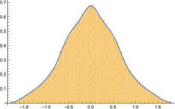
Figure 1 y = f 6 ^ ( 12 , 50 ) ( x ) 𝑦 superscript ^ subscript 𝑓 6 12 50 𝑥 y=\widehat{f_{6}}^{(12,50)}(x) b 1 absent subscript 𝑏 1 \sqrt{\vrule width=0.0pt,height=5.16663pt}{b_{1}} 10 6 superscript 10 6 10^{6}
Table 5: Fourier coefficients a n , k ^ ( 50 ) ( n = 4 , 6 , 8 , 10 ) superscript ^ subscript 𝑎 𝑛 𝑘
50 𝑛 4 6 8 10
\widehat{a_{n,k}}^{(50)}\quad\quad(n=4,6,8,10)
k n = 4 n = 6 n = 8 n = 10 0 8.66025 × 10 − 1 5.59017 × 10 − 1 4.40959 × 10 − 1 3.75000 × 10 − 1 1 1.76257 × 10 − 1 3.08052 × 10 − 1 3.12106 × 10 − 1 2.97971 × 10 − 1 2 7.26283 × 10 − 2 5.75070 × 10 − 2 1.18300 × 10 − 1 1.55596 × 10 − 1 3 5.56174 × 10 − 2 1.17190 × 10 − 2 3.20582 × 10 − 2 6.04639 × 10 − 2 4 3.80806 × 10 − 2 − 5.99392 × 10 − 3 6.29481 × 10 − 3 1.95825 × 10 − 2 5 3.28048 × 10 − 2 6.78429 × 10 − 3 1.54291 × 10 − 3 5.48500 × 10 − 3 6 2.57761 × 10 − 2 7.71527 × 10 − 3 4.84745 × 10 − 4 1.49687 × 10 − 3 7 2.32437 × 10 − 2 6.95419 × 10 − 3 − 5.28008 × 10 − 4 2.86985 × 10 − 4 8 1.94759 × 10 − 2 1.62249 × 10 − 4 − 2.89091 × 10 − 4 5.48249 × 10 − 5 9 1.79941 × 10 − 2 2.38820 × 10 − 5 6.47841 × 10 − 4 7.54897 × 10 − 5 10 1.56490 × 10 − 2 6.33581 × 10 − 4 1.01858 × 10 − 3 2.55678 × 10 − 5 11 1.46777 × 10 − 2 3.10573 × 10 − 3 6.95872 × 10 − 4 − 7.05180 × 10 − 5 12 1.33900 × 10 − 2 1.73510 × 10 − 3 3.76670 × 10 − 4 − 5.51200 × 10 − 5 𝑘 𝑛 4 𝑛 6 𝑛 8 𝑛 10 missing-subexpression missing-subexpression missing-subexpression missing-subexpression missing-subexpression 0 8.66025 superscript 10 1 5.59017 superscript 10 1 4.40959 superscript 10 1 3.75000 superscript 10 1 1 1.76257 superscript 10 1 3.08052 superscript 10 1 3.12106 superscript 10 1 2.97971 superscript 10 1 2 7.26283 superscript 10 2 5.75070 superscript 10 2 1.18300 superscript 10 1 1.55596 superscript 10 1 3 5.56174 superscript 10 2 1.17190 superscript 10 2 3.20582 superscript 10 2 6.04639 superscript 10 2 4 3.80806 superscript 10 2 5.99392 superscript 10 3 6.29481 superscript 10 3 1.95825 superscript 10 2 5 3.28048 superscript 10 2 6.78429 superscript 10 3 1.54291 superscript 10 3 5.48500 superscript 10 3 6 2.57761 superscript 10 2 7.71527 superscript 10 3 4.84745 superscript 10 4 1.49687 superscript 10 3 7 2.32437 superscript 10 2 6.95419 superscript 10 3 5.28008 superscript 10 4 2.86985 superscript 10 4 8 1.94759 superscript 10 2 1.62249 superscript 10 4 2.89091 superscript 10 4 5.48249 superscript 10 5 9 1.79941 superscript 10 2 2.38820 superscript 10 5 6.47841 superscript 10 4 7.54897 superscript 10 5 10 1.56490 superscript 10 2 6.33581 superscript 10 4 1.01858 superscript 10 3 2.55678 superscript 10 5 11 1.46777 superscript 10 2 3.10573 superscript 10 3 6.95872 superscript 10 4 7.05180 superscript 10 5 12 1.33900 superscript 10 2 1.73510 superscript 10 3 3.76670 superscript 10 4 5.51200 superscript 10 5 \begin{array}[]{rrrrr}k&n=4&n=6&n=8&n=10\\
\hline\cr 0&8.66025\times 10^{-1}&5.59017\times 10^{-1}&4.40959\times 10^{-1}&3.75000\times 10^{-1}\\
1&1.76257\times 10^{-1}&3.08052\times 10^{-1}&3.12106\times 10^{-1}&2.97971\times 10^{-1}\\
2&7.26283\times 10^{-2}&5.75070\times 10^{-2}&1.18300\times 10^{-1}&1.55596\times 10^{-1}\\
3&5.56174\times 10^{-2}&1.17190\times 10^{-2}&3.20582\times 10^{-2}&6.04639\times 10^{-2}\\
4&3.80806\times 10^{-2}&-5.99392\times 10^{-3}&6.29481\times 10^{-3}&1.95825\times 10^{-2}\\
5&3.28048\times 10^{-2}&6.78429\times 10^{-3}&1.54291\times 10^{-3}&5.48500\times 10^{-3}\\
6&2.57761\times 10^{-2}&7.71527\times 10^{-3}&4.84745\times 10^{-4}&1.49687\times 10^{-3}\\
7&2.32437\times 10^{-2}&6.95419\times 10^{-3}&-5.28008\times 10^{-4}&2.86985\times 10^{-4}\\
8&1.94759\times 10^{-2}&1.62249\times 10^{-4}&-2.89091\times 10^{-4}&5.48249\times 10^{-5}\\
9&1.79941\times 10^{-2}&2.38820\times 10^{-5}&6.47841\times 10^{-4}&7.54897\times 10^{-5}\\
10&1.56490\times 10^{-2}&6.33581\times 10^{-4}&1.01858\times 10^{-3}&2.55678\times 10^{-5}\\
11&1.46777\times 10^{-2}&3.10573\times 10^{-3}&6.95872\times 10^{-4}&-7.05180\times 10^{-5}\\
12&1.33900\times 10^{-2}&1.73510\times 10^{-3}&3.76670\times 10^{-4}&-5.51200\times 10^{-5}\\
\end{array}
Table 6: Fourier coefficients a n , k ^ ( 50 ) ( n = 12 , 14 , 16 , 18 ) superscript ^ subscript 𝑎 𝑛 𝑘
50 𝑛 12 14 16 18
\widehat{a_{n,k}}^{(50)}\quad(n=12,14,16,18)
k n = 12 n = 14 n = 16 n = 18 0 3.31662 × 10 − 1 3.00463 × 10 − 1 2.76642 × 10 − 1 2.57694 × 10 − 1 1 2.81214 × 10 − 1 2.65297 × 10 − 1 2.50979 × 10 − 1 2.38295 × 10 − 1 2 1.75649 × 10 − 1 1.85442 × 10 − 1 1.89288 × 10 − 1 1.89688 × 10 − 1 3 8.64878 × 10 − 2 1.06921 × 10 − 1 1.21861 × 10 − 1 1.32313 × 10 − 1 4 3.61873 × 10 − 2 5.33942 × 10 − 2 6.92058 × 10 − 2 8.27429 × 10 − 2 5 1.34095 × 10 − 2 2.39311 × 10 − 2 3.56438 × 10 − 2 4.73779 × 10 − 2 6 4.55324 × 10 − 3 9.85304 × 10 − 3 1.69758 × 10 − 2 2.52441 × 10 − 2 7 1.43298 × 10 − 3 3.79153 × 10 − 3 7.58376 × 10 − 3 1.26687 × 10 − 2 8 4.17297 × 10 − 4 1.37582 × 10 − 3 3.21053 × 10 − 3 6.04348 × 10 − 3 9 1.25392 × 10 − 4 4.76811 × 10 − 4 1.29802 × 10 − 3 2.75976 × 10 − 3 10 3.65441 × 10 − 5 1.59551 × 10 − 4 5.04694 × 10 − 4 1.21325 × 10 − 3 11 1.38971 × 10 − 6 5.02895 × 10 − 5 1.89440 × 10 − 4 5.15815 × 10 − 4 12 − 1.40240 × 10 − 6 1.49690 × 10 − 5 6.87622 × 10 − 5 2.12808 × 10 − 4 𝑘 𝑛 12 𝑛 14 𝑛 16 𝑛 18 missing-subexpression missing-subexpression missing-subexpression missing-subexpression missing-subexpression 0 3.31662 superscript 10 1 3.00463 superscript 10 1 2.76642 superscript 10 1 2.57694 superscript 10 1 1 2.81214 superscript 10 1 2.65297 superscript 10 1 2.50979 superscript 10 1 2.38295 superscript 10 1 2 1.75649 superscript 10 1 1.85442 superscript 10 1 1.89288 superscript 10 1 1.89688 superscript 10 1 3 8.64878 superscript 10 2 1.06921 superscript 10 1 1.21861 superscript 10 1 1.32313 superscript 10 1 4 3.61873 superscript 10 2 5.33942 superscript 10 2 6.92058 superscript 10 2 8.27429 superscript 10 2 5 1.34095 superscript 10 2 2.39311 superscript 10 2 3.56438 superscript 10 2 4.73779 superscript 10 2 6 4.55324 superscript 10 3 9.85304 superscript 10 3 1.69758 superscript 10 2 2.52441 superscript 10 2 7 1.43298 superscript 10 3 3.79153 superscript 10 3 7.58376 superscript 10 3 1.26687 superscript 10 2 8 4.17297 superscript 10 4 1.37582 superscript 10 3 3.21053 superscript 10 3 6.04348 superscript 10 3 9 1.25392 superscript 10 4 4.76811 superscript 10 4 1.29802 superscript 10 3 2.75976 superscript 10 3 10 3.65441 superscript 10 5 1.59551 superscript 10 4 5.04694 superscript 10 4 1.21325 superscript 10 3 11 1.38971 superscript 10 6 5.02895 superscript 10 5 1.89440 superscript 10 4 5.15815 superscript 10 4 12 1.40240 superscript 10 6 1.49690 superscript 10 5 6.87622 superscript 10 5 2.12808 superscript 10 4 \begin{array}[]{rrrrr}k&n=12&n=14&n=16&n=18\\
\hline\cr 0&3.31662\times 10^{-1}&3.00463\times 10^{-1}&2.76642\times 10^{-1}&2.57694\times 10^{-1}\\
1&2.81214\times 10^{-1}&2.65297\times 10^{-1}&2.50979\times 10^{-1}&2.38295\times 10^{-1}\\
2&1.75649\times 10^{-1}&1.85442\times 10^{-1}&1.89288\times 10^{-1}&1.89688\times 10^{-1}\\
3&8.64878\times 10^{-2}&1.06921\times 10^{-1}&1.21861\times 10^{-1}&1.32313\times 10^{-1}\\
4&3.61873\times 10^{-2}&5.33942\times 10^{-2}&6.92058\times 10^{-2}&8.27429\times 10^{-2}\\
5&1.34095\times 10^{-2}&2.39311\times 10^{-2}&3.56438\times 10^{-2}&4.73779\times 10^{-2}\\
6&4.55324\times 10^{-3}&9.85304\times 10^{-3}&1.69758\times 10^{-2}&2.52441\times 10^{-2}\\
7&1.43298\times 10^{-3}&3.79153\times 10^{-3}&7.58376\times 10^{-3}&1.26687\times 10^{-2}\\
8&4.17297\times 10^{-4}&1.37582\times 10^{-3}&3.21053\times 10^{-3}&6.04348\times 10^{-3}\\
9&1.25392\times 10^{-4}&4.76811\times 10^{-4}&1.29802\times 10^{-3}&2.75976\times 10^{-3}\\
10&3.65441\times 10^{-5}&1.59551\times 10^{-4}&5.04694\times 10^{-4}&1.21325\times 10^{-3}\\
11&1.38971\times 10^{-6}&5.02895\times 10^{-5}&1.89440\times 10^{-4}&5.15815\times 10^{-4}\\
12&-1.40240\times 10^{-6}&1.49690\times 10^{-5}&6.87622\times 10^{-5}&2.12808\times 10^{-4}\\
\end{array}
Table 7: Fourier coefficients a n , k ^ ( 50 ) ( n = 20 , 22 ) superscript ^ subscript 𝑎 𝑛 𝑘
50 𝑛 20 22
\widehat{a_{n,k}}^{(50)}\quad(n=20,22)
k n = 20 n = 22 0 2.42161 × 10 − 1 2.29129 × 10 − 1 1 2.27078 × 10 − 1 2.17130 × 10 − 1 2 1.88097 × 10 − 1 1.85373 × 10 − 1 3 1.39342 × 10 − 1 1.43837 × 10 − 1 4 9.38340 × 10 − 2 1.02652 × 10 − 1 5 5.83684 × 10 − 2 6.82124 × 10 − 2 6 3.39847 × 10 − 2 4.26601 × 10 − 2 7 1.87134 × 10 − 2 2.53303 × 10 − 2 8 9.82378 × 10 − 3 1.43802 × 10 − 2 9 4.94778 × 10 − 3 7.84948 × 10 − 3 10 2.40299 × 10 − 3 4.13869 × 10 − 3 11 1.13008 × 10 − 3 2.11578 × 10 − 3 12 5.16361 × 10 − 4 1.05205 × 10 − 3 𝑘 𝑛 20 𝑛 22 missing-subexpression missing-subexpression missing-subexpression 0 2.42161 superscript 10 1 2.29129 superscript 10 1 1 2.27078 superscript 10 1 2.17130 superscript 10 1 2 1.88097 superscript 10 1 1.85373 superscript 10 1 3 1.39342 superscript 10 1 1.43837 superscript 10 1 4 9.38340 superscript 10 2 1.02652 superscript 10 1 5 5.83684 superscript 10 2 6.82124 superscript 10 2 6 3.39847 superscript 10 2 4.26601 superscript 10 2 7 1.87134 superscript 10 2 2.53303 superscript 10 2 8 9.82378 superscript 10 3 1.43802 superscript 10 2 9 4.94778 superscript 10 3 7.84948 superscript 10 3 10 2.40299 superscript 10 3 4.13869 superscript 10 3 11 1.13008 superscript 10 3 2.11578 superscript 10 3 12 5.16361 superscript 10 4 1.05205 superscript 10 3 \begin{array}[]{rrr}k&n=20&n=22\\
\hline\cr 0&2.42161\times 10^{-1}&2.29129\times 10^{-1}\\
1&2.27078\times 10^{-1}&2.17130\times 10^{-1}\\
2&1.88097\times 10^{-1}&1.85373\times 10^{-1}\\
3&1.39342\times 10^{-1}&1.43837\times 10^{-1}\\
4&9.38340\times 10^{-2}&1.02652\times 10^{-1}\\
5&5.83684\times 10^{-2}&6.82124\times 10^{-2}\\
6&3.39847\times 10^{-2}&4.26601\times 10^{-2}\\
7&1.87134\times 10^{-2}&2.53303\times 10^{-2}\\
8&9.82378\times 10^{-3}&1.43802\times 10^{-2}\\
9&4.94778\times 10^{-3}&7.84948\times 10^{-3}\\
10&2.40299\times 10^{-3}&4.13869\times 10^{-3}\\
11&1.13008\times 10^{-3}&2.11578\times 10^{-3}\\
12&5.16361\times 10^{-4}&1.05205\times 10^{-3}\\
\end{array}
Figure 1: Plot of y = f 6 ^ ( 12 , 50 ) ( x ) 𝑦 superscript ^ subscript 𝑓 6 12 50 𝑥 y=\widehat{f_{6}}^{(12,50)}(x) b 1 absent subscript 𝑏 1 \sqrt{\vrule width=0.0pt,height=5.16663pt}{b_{1}} 10 6 superscript 10 6 10^{6}
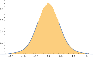
We now illustrate the case n = 20 𝑛 20 n=20 2
f 20 ^ ( 12 , 50 ) ( x ) = superscript ^ subscript 𝑓 20 12 50 𝑥 absent \displaystyle\widehat{f_{20}}^{(12,50)}(x)\,= 1.21081 × 10 − 1 + ( 2.27078 × 10 − 1 ) cos ( 1 18 19 π x ) 1.21081 superscript 10 1 2.27078 superscript 10 1 1 18 19 𝜋 𝑥 \displaystyle\,\,1.21081\times 10^{-1}+\left(2.27078\times 10^{-1}\right)\cos\left(\frac{1}{18}\sqrt{19}\pi x\right)
+ ( 1.88097 × 10 − 1 ) cos ( 1 9 19 π x ) + ( 1.39342 × 10 − 1 ) cos ( 1 6 19 π x ) 1.88097 superscript 10 1 1 9 19 𝜋 𝑥 1.39342 superscript 10 1 1 6 19 𝜋 𝑥 \displaystyle+\left(1.88097\times 10^{-1}\right)\cos\left(\frac{1}{9}\sqrt{19}\pi x\right)+\left(1.39342\times 10^{-1}\right)\cos\left(\frac{1}{6}\sqrt{19}\pi x\right)
+ ( 9.38340 × 10 − 2 ) cos ( 2 9 19 π x ) + ( 5.83684 × 10 − 2 ) cos ( 5 18 19 π x ) 9.38340 superscript 10 2 2 9 19 𝜋 𝑥 5.83684 superscript 10 2 5 18 19 𝜋 𝑥 \displaystyle+\left(9.38340\times 10^{-2}\right)\cos\left(\frac{2}{9}\sqrt{19}\pi x\right)+\left(5.83684\times 10^{-2}\right)\cos\left(\frac{5}{18}\sqrt{19}\pi x\right)
+ ( 3.39847 × 10 − 2 ) cos ( 1 3 19 π x ) + ( 1.87134 × 10 − 2 ) cos ( 7 18 19 π x ) 3.39847 superscript 10 2 1 3 19 𝜋 𝑥 1.87134 superscript 10 2 7 18 19 𝜋 𝑥 \displaystyle+\left(3.39847\times 10^{-2}\right)\cos\left(\frac{1}{3}\sqrt{19}\pi x\right)+\left(1.87134\times 10^{-2}\right)\cos\left(\frac{7}{18}\sqrt{19}\pi x\right)
+ ( 9.82378 × 10 − 3 ) cos ( 4 9 19 π x ) + ( 4.94778 × 10 − 3 ) cos ( 1 2 19 π x ) 9.82378 superscript 10 3 4 9 19 𝜋 𝑥 4.94778 superscript 10 3 1 2 19 𝜋 𝑥 \displaystyle+\left(9.82378\times 10^{-3}\right)\cos\left(\frac{4}{9}\sqrt{19}\pi x\right)+\left(4.94778\times 10^{-3}\right)\cos\left(\frac{1}{2}\sqrt{19}\pi x\right)
+ ( 2.40299 × 10 − 3 ) cos ( 5 9 19 π x ) + ( 1.13008 × 10 − 3 ) cos ( 11 18 19 π x ) 2.40299 superscript 10 3 5 9 19 𝜋 𝑥 1.13008 superscript 10 3 11 18 19 𝜋 𝑥 \displaystyle+\left(2.40299\times 10^{-3}\right)\cos\left(\frac{5}{9}\sqrt{19}\pi x\right)+\left(1.13008\times 10^{-3}\right)\cos\left(\frac{11}{18}\sqrt{19}\pi x\right)
+ ( 5.16361 × 10 − 4 ) cos ( 2 3 19 π x ) 5.16361 superscript 10 4 2 3 19 𝜋 𝑥 \displaystyle+\left(5.16361\times 10^{-4}\right)\cos\left(\frac{2}{3}\sqrt{19}\pi x\right)
and
F 20 ^ ( 12 , 50 ) ( x ) = superscript ^ subscript 𝐹 20 12 50 𝑥 absent \displaystyle\widehat{F_{20}}^{(12,50)}(x)\,= 1 2 ( 19 x 18 + 1 ) + ( 2.98484 × 10 − 1 ) sin ( 1 18 19 π x ) 1 2 19 𝑥 18 1 2.98484 superscript 10 1 1 18 19 𝜋 𝑥 \displaystyle\,\,\frac{1}{2}\left(\frac{\sqrt{19}x}{18}+1\right)+\left(2.98484\times 10^{-1}\right)\sin\left(\frac{1}{18}\sqrt{19}\pi x\right)
+ ( 1.23623 × 10 − 1 ) sin ( 1 9 19 π x ) + ( 6.10528 × 10 − 2 ) sin ( 1 6 19 π x ) 1.23623 superscript 10 1 1 9 19 𝜋 𝑥 6.10528 superscript 10 2 1 6 19 𝜋 𝑥 \displaystyle+\left(1.23623\times 10^{-1}\right)\sin\left(\frac{1}{9}\sqrt{19}\pi x\right)+\left(6.10528\times 10^{-2}\right)\sin\left(\frac{1}{6}\sqrt{19}\pi x\right)
+ ( 3.08352 × 10 − 2 ) sin ( 2 9 19 π x ) + ( 1.53445 × 10 − 2 ) sin ( 5 18 19 π x ) 3.08352 superscript 10 2 2 9 19 𝜋 𝑥 1.53445 superscript 10 2 5 18 19 𝜋 𝑥 \displaystyle+\left(3.08352\times 10^{-2}\right)\sin\left(\frac{2}{9}\sqrt{19}\pi x\right)+\left(1.53445\times 10^{-2}\right)\sin\left(\frac{5}{18}\sqrt{19}\pi x\right)
+ ( 7.44524 × 10 − 3 ) sin ( 1 3 19 π x ) + ( 3.51399 × 10 − 3 ) sin ( 7 18 19 π x ) 7.44524 superscript 10 3 1 3 19 𝜋 𝑥 3.51399 superscript 10 3 7 18 19 𝜋 𝑥 \displaystyle+\left(7.44524\times 10^{-3}\right)\sin\left(\frac{1}{3}\sqrt{19}\pi x\right)+\left(3.51399\times 10^{-3}\right)\sin\left(\frac{7}{18}\sqrt{19}\pi x\right)
+ ( 1.61412 × 10 − 3 ) sin ( 4 9 19 π x ) + ( 7.22627 × 10 − 4 ) sin ( 1 2 19 π x ) 1.61412 superscript 10 3 4 9 19 𝜋 𝑥 7.22627 superscript 10 4 1 2 19 𝜋 𝑥 \displaystyle+\left(1.61412\times 10^{-3}\right)\sin\left(\frac{4}{9}\sqrt{19}\pi x\right)+\left(7.22627\times 10^{-4}\right)\sin\left(\frac{1}{2}\sqrt{19}\pi x\right)
+ ( 3.15863 × 10 − 4 ) sin ( 5 9 19 π x ) + ( 1.35040 × 10 − 4 ) sin ( 11 18 19 π x ) 3.15863 superscript 10 4 5 9 19 𝜋 𝑥 1.35040 superscript 10 4 11 18 19 𝜋 𝑥 \displaystyle+\left(3.15863\times 10^{-4}\right)\sin\left(\frac{5}{9}\sqrt{19}\pi x\right)+\left(1.35040\times 10^{-4}\right)\sin\left(\frac{11}{18}\sqrt{19}\pi x\right)
+ ( 5.65611 × 10 − 5 ) sin ( 2 3 19 π x ) . 5.65611 superscript 10 5 2 3 19 𝜋 𝑥 \displaystyle+\left(5.65611\times 10^{-5}\right)\sin\left(\frac{2}{3}\sqrt{19}\pi x\right).
Figure 2: Plot of y = f 20 ^ ( 12 , 50 ) ( x ) 𝑦 superscript ^ subscript 𝑓 20 12 50 𝑥 y=\widehat{f_{20}}^{(12,50)}(x) b 1 absent subscript 𝑏 1 \sqrt{\vrule width=0.0pt,height=5.16663pt}{b_{1}} 10 6 superscript 10 6 10^{6}
Tables 8 9 1 − F 20 ^ ( 12 , 50 ) ( x ) 1 superscript ^ subscript 𝐹 20 12 50 𝑥 1-\widehat{F_{20}}^{(12,50)}(x) x α subscript 𝑥 𝛼 x_{\alpha} α = 0.900 , 0.950 , 0.975 , 0.990.0.995 , 0.999 𝛼 0.900 0.950 0.975 0.990.0.995 0.999
\alpha=0.900,0.950,0.975,0.990.0.995,0.999 x α subscript 𝑥 𝛼 x_{\alpha} F 20 ^ ( 12 , 50 ) ( x α ) = α superscript ^ subscript 𝐹 20 12 50 subscript 𝑥 𝛼 𝛼 \widehat{F_{20}}^{(12,50)}(x_{\alpha})=\alpha [7 ] .
Table 8: Upper tail probability 1 − F n ^ ( 12 , 50 ) ( x ) 1 superscript ^ subscript 𝐹 𝑛 12 50 𝑥 1-\widehat{F_{n}}^{(12,50)}(x) b 1 absent subscript 𝑏 1 \sqrt{\vrule width=0.0pt,height=5.16663pt}{b_{1}}
x n = 4 n = 6 n = 8 n = 10 n = 12 0.1 0.41 78 ¯ 0.4332 0.4311 0.4276 0.4240 0.2 0.3 604 ¯ 0.370 5 ¯ 0.3648 0.3579 0.3511 0.3 0.308 3 ¯ 0.312 3 ¯ 0.302 8 ¯ 0.2932 0.2839 0.4 0.26 31 ¯ 0.258 3 ¯ 0.2464 0.2352 0.2244 0.5 0.220 7 ¯ 0.209 3 ¯ 0.1967 0.1849 0.1736 0.6 0.1818 0.165 3 ¯ 0.1544 0.1427 0.1316 0.7 0.1451 0.127 9 ¯ 0.1194 0.1082 0.0979 0.8 0.110 3 ¯ 0.098 6 ¯ 0.0907 0.080 8 ¯ 0.0717 0.9 0.077 6 ¯ 0.075 6 ¯ 0.067 6 ¯ 0.0594 0.0517 1.0 0.04 59 ¯ 0.0567 0.0496 0.0430 0.0368 1.1 0.016 2 ¯ 0.0414 0.0359 0.0307 0.0258 1.2 – 0.0291 0.0257 0.0217 0.0179 1.3 – 0.0193 0.0181 0.0150 0.0123 1.4 – 0.0118 0.0124 0.0103 0.0083 1.5 – 0.0063 0.0082 0.0069 0.0056 1.6 – 0.0026 0.0051 0.0046 0.0037 1.7 – 0.0006 0.0030 0.0029 0.0024 1.8 – – 0.0016 0.0018 0.0015 1.9 – – 0.0008 0.0010 0.0009 2.0 – – 0.0003 0.0006 0.0005 𝑥 𝑛 4 𝑛 6 𝑛 8 𝑛 10 𝑛 12 missing-subexpression missing-subexpression missing-subexpression missing-subexpression missing-subexpression missing-subexpression 0.1 0.41 ¯ 78 0.4332 0.4311 0.4276 0.4240 0.2 0.3 ¯ 604 0.370 ¯ 5 0.3648 0.3579 0.3511 0.3 0.308 ¯ 3 0.312 ¯ 3 0.302 ¯ 8 0.2932 0.2839 0.4 0.26 ¯ 31 0.258 ¯ 3 0.2464 0.2352 0.2244 0.5 0.220 ¯ 7 0.209 ¯ 3 0.1967 0.1849 0.1736 0.6 0.1818 0.165 ¯ 3 0.1544 0.1427 0.1316 0.7 0.1451 0.127 ¯ 9 0.1194 0.1082 0.0979 0.8 0.110 ¯ 3 0.098 ¯ 6 0.0907 0.080 ¯ 8 0.0717 0.9 0.077 ¯ 6 0.075 ¯ 6 0.067 ¯ 6 0.0594 0.0517 1.0 0.04 ¯ 59 0.0567 0.0496 0.0430 0.0368 1.1 0.016 ¯ 2 0.0414 0.0359 0.0307 0.0258 1.2 – 0.0291 0.0257 0.0217 0.0179 1.3 – 0.0193 0.0181 0.0150 0.0123 1.4 – 0.0118 0.0124 0.0103 0.0083 1.5 – 0.0063 0.0082 0.0069 0.0056 1.6 – 0.0026 0.0051 0.0046 0.0037 1.7 – 0.0006 0.0030 0.0029 0.0024 1.8 – – 0.0016 0.0018 0.0015 1.9 – – 0.0008 0.0010 0.0009 2.0 – – 0.0003 0.0006 0.0005 \begin{array}[]{rrrrrr}x&n=4&n=6&n=8&n=10&n=12\\
\hline\cr 0.1&0.41\underline{78}&0.4332&0.4311&0.4276&0.4240\\
0.2&0.3\underline{604}&0.370\underline{5}&0.3648&0.3579&0.3511\\
0.3&0.308\underline{3}&0.312\underline{3}&0.302\underline{8}&0.2932&0.2839\\
0.4&0.26\underline{31}&0.258\underline{3}&0.2464&0.2352&0.2244\\
0.5&0.220\underline{7}&0.209\underline{3}&0.1967&0.1849&0.1736\\
0.6&0.1818&0.165\underline{3}&0.1544&0.1427&0.1316\\
0.7&0.1451&0.127\underline{9}&0.1194&0.1082&0.0979\\
0.8&0.110\underline{3}&0.098\underline{6}&0.0907&0.080\underline{8}&0.0717\\
0.9&0.077\underline{6}&0.075\underline{6}&0.067\underline{6}&0.0594&0.0517\\
1.0&0.04\underline{59}&0.0567&0.0496&0.0430&0.0368\\
1.1&0.016\underline{2}&0.0414&0.0359&0.0307&0.0258\\
1.2&\text{--}&0.0291&0.0257&0.0217&0.0179\\
1.3&\text{--}&0.0193&0.0181&0.0150&0.0123\\
1.4&\text{--}&0.0118&0.0124&0.0103&0.0083\\
1.5&\text{--}&0.0063&0.0082&0.0069&0.0056\\
1.6&\text{--}&0.0026&0.0051&0.0046&0.0037\\
1.7&\text{--}&0.0006&0.0030&0.0029&0.0024\\
1.8&\text{--}&\text{--}&0.0016&0.0018&0.0015\\
1.9&\text{--}&\text{--}&0.0008&0.0010&0.0009\\
2.0&\text{--}&\text{--}&0.0003&0.0006&0.0005\\
\end{array}
Table 9: Upper percentiles x α subscript 𝑥 𝛼 x_{\alpha} b 1 absent subscript 𝑏 1 \sqrt{\vrule width=0.0pt,height=5.16663pt}{b_{1}}
n α 0.900 0.950 0.975 0.990 0.995 0.999 4 0.8305 0.9869 1.0697 1.12 10 ¯ 1.13 79 ¯ 1.1513 6 0.7945 1.04 12 ¯ 1.2392 1.4299 1.5306 1.6707 8 0.7652 0.9977 1.2080 1.4524 1.6046 1.8668 10 0.7275 0.9539 1.1595 1.4075 1.5785 1.9065 12 0.6931 0.9100 1.1091 1.3532 1.5255 1.8818 14 0.6622 0.8699 1.0614 1.2985 1.4683 1.8315 16 0.6347 0.8337 1.0176 1.2467 1.4121 1.7739 18 0.6102 0.8012 0.9778 1.1988 1.3595 1.71 33 ¯ 20 0.5881 0.7721 0.9419 1.15 43 ¯ 1.31 08 ¯ 1.65 20 ¯ 22 0.5681 0.7459 0.90 97 ¯ 1.11 30 ¯ 1.26 37 ¯ 1.60 45 ¯ 𝑛 𝛼 missing-subexpression missing-subexpression missing-subexpression missing-subexpression missing-subexpression missing-subexpression missing-subexpression missing-subexpression 0.900 0.950 0.975 0.990 0.995 0.999 missing-subexpression missing-subexpression missing-subexpression missing-subexpression missing-subexpression missing-subexpression missing-subexpression 4 0.8305 0.9869 1.0697 1.12 ¯ 10 1.13 ¯ 79 1.1513 6 0.7945 1.04 ¯ 12 1.2392 1.4299 1.5306 1.6707 8 0.7652 0.9977 1.2080 1.4524 1.6046 1.8668 10 0.7275 0.9539 1.1595 1.4075 1.5785 1.9065 12 0.6931 0.9100 1.1091 1.3532 1.5255 1.8818 14 0.6622 0.8699 1.0614 1.2985 1.4683 1.8315 16 0.6347 0.8337 1.0176 1.2467 1.4121 1.7739 18 0.6102 0.8012 0.9778 1.1988 1.3595 1.71 ¯ 33 20 0.5881 0.7721 0.9419 1.15 ¯ 43 1.31 ¯ 08 1.65 ¯ 20 22 0.5681 0.7459 0.90 ¯ 97 1.11 ¯ 30 1.26 ¯ 37 1.60 ¯ 45 \begin{array}[]{rrrrrrr}n&\lx@intercol\hfil\alpha\hfil\lx@intercol\\
\hline\cr&0.900&0.950&0.975&0.990&0.995&0.999\\
\hline\cr 4&0.8305&0.9869&1.0697&1.12\underline{10}&1.13\underline{79}&1.1513\\
6&0.7945&1.04\underline{12}&1.2392&1.4299&1.5306&1.6707\\
8&0.7652&0.9977&1.2080&1.4524&1.6046&1.8668\\
10&0.7275&0.9539&1.1595&1.4075&1.5785&1.9065\\
12&0.6931&0.9100&1.1091&1.3532&1.5255&1.8818\\
14&0.6622&0.8699&1.0614&1.2985&1.4683&1.8315\\
16&0.6347&0.8337&1.0176&1.2467&1.4121&1.7739\\
18&0.6102&0.8012&0.9778&1.1988&1.3595&1.71\underline{33}\\
20&0.5881&0.7721&0.9419&1.15\underline{43}&1.31\underline{08}&1.65\underline{20}\\
22&0.5681&0.7459&0.90\underline{97}&1.11\underline{30}&1.26\underline{37}&1.60\underline{45}\\
\end{array}