Interpreting Deep Learning Models with
Marginal Attribution by Conditioning on Quantiles

Abstract

A vastly growing literature on explaining deep learning models has emerged. This paper contributes to that literature by introducing a global gradient-based model-agnostic method, which we call Marginal Attribution by Conditioning on Quantiles (MACQ). Our approach is based on analyzing the marginal attribution of predictions (outputs) to individual features (inputs). Specifically, we consider variable importance by fixing (global) output levels and, thus, explain how features marginally contribute across different regions of the prediction space. Hence, MACQ can be seen as a marginal attribution counterpart to approaches such as accumulated local effects (ALE), which study the sensitivities of outputs by perturbing inputs. Furthermore, MACQ allows us to separate marginal attribution of individual features from interaction effect, and visually illustrate the 3-way relationship between marginal attribution, output level, and feature value.

Keywords. explainable AI (XAI), model-agnostic tools, deep learning, attribution, accumulated local effects (ALE), partial dependence plot (PDP), locally interpretable model-agnostic explanation (LIME), variable importance, post-hoc analysis.

1 Introduction

Deep learning models are typically trained to provide an optimal predictive performance. Interpreting and explaining the results of deep learning models has, until recently, only played a subordinate role. With growing complexity of deep learning models, the need and requirement of being able to explain deep learning solutions has become increasingly important. This applies to almost all fields of their applications: deep learning findings in medical fields and health care need to make sense to patients, loan and mortgage evaluations and credit approvals need to be understandable to customers, insurance pricing must be explained to insurance policyholders, business processes and decisions need to be transparent to regulators, autonomous robotic tools need to comply with safety standards according to admission offices and governments, etc. These needs are even reinforced by the requirements of being able to prove that deep learning solutions do not discriminate w.r.t. protected features and are in line with data protection regulation. Thus, there is substantial social and political pressure to be able to explain, illustrate and verify deep learning solutions, in order to provide reassurance that these work properly.

Recent research focuses on different methods of explaining deep learning decision making; an overview is given in [Samek and Müller 2019]. Some of these methods provide a post-hoc analysis which aims at understanding global model behavior, explaining individual outcomes and learned representations. Often this is done by explaining representative examples. We are going to discuss some of these post-hoc analysis methods in the literature overview presented in the next section. Other methods aim at a wider interdisciplinary approach by more broadly examining how decision making is done in a social context, see e.g. [Miller 2019]. All these approaches have in common that they try to “open up the black-box” to make decision making explainable to stakeholders.

Our paper contributes to this literature. Our main contribution is that we provide a novel gradient-based model-agnostic tool that is motivated by analyzing marginal contributions to deep learning decisions in the spirit of salience methods, as described in [Ancona et al. 2019]. Salience methods are local model-agnostic tools that attribute marginal effects on outputs to different inputs. Motivated by sensitivity analysis tools in risk measurement, we aggregate local marginal attributions to obtain a global picture at a given quantile level of the output variable. We call this method Marginal Attribution by Conditioning on Quantiles (MACQ). It describes a global variable importance measure that varies with the output level. The aggregation of local marginal effects is justified by the fact that this aggregation can be seen as a directional derivative of a distortion risk measure, see [Hong 2009] and Proposition 1 in [Tsanakas and Millossovich 2015]. As second contribution, we extend this view by including higher order derivatives beyond linear marginal contributions. This additional step can be seen in the context of deep Taylor decompositions (DTD), similar to [Montavon et al. 2017]. A difficulty in Taylor decompositions is that they depend on a reference point. By rearranging the terms and by taking advantage of our quantile view, we determine an optimal global reference point that allows us to quantify both variable importance and interaction strength in our MACQ approach. The third contribution is that we provide graphic tools that provide a 3-way relationship between (i) marginal attribution, (ii) response/output level and (iii) feature value.

Organization. In the next section we give a literature overview that embeds our MACQ method into the present toolbox of model explainability. This literature overview is also used to introduce the relevant notation. In Section 3 we present our main idea of aggregating local marginal attributions to a quantile sensitivity analysis. Section 4 presents a higher order expansion which grounds a study of interaction strength. Section 5 discusses the choice of the reference point. An extended example is presented in Section 6. Finally, in Section 7 we state brief conclusions.

2 Literature overview

We give a brief summary of recent developments in post-hoc interpretability and explainability tools for deep learning models. This summary also serves to introduce the relevant notation for this paper. Assume the following regression function is smooth (in fact, we are only going to use twice differentiable in our setting)

$$\mu:{\mathbb{R}}^{q}\to{\mathbb{R}},\qquad\boldsymbol{x}\mapsto\mu(\boldsymbol{x}),$$ (2.1)

with feature $\boldsymbol{x}=(x_{1},\ldots,x_{q})^{\top}\in{\mathbb{R}}^{q}$. This regression function is assumed to describe the systematic effects of features on the random variable $Y$ via the (conditional) expectation

$${\mathbb{E}}[Y|\boldsymbol{x}]=\mu(\boldsymbol{x}).$$

We assume smoothness of regression function (2.1) because our model-agnostic proposal will be gradient-based. In our example in Section 6, we will use a deep feed-forward neural network on tabular input data, having the hyperbolic tangent as activation function. This gives us a smooth regression function and formal derivation can be done in standard software such as TensorFlow/Keras and PyTorch.

2.1 Model-agnostic tools

Recent literature aims understanding such regression functions (2.1) coming from deep learning models. One approach is to analyze marginal plots. We select one component $x_{j}$ of $\boldsymbol{x}$ and study the function

$$x_{j}\in{\mathbb{R}}~{}\mapsto~{}\mu(x_{j},\boldsymbol{x}_{\setminus j}),$$

where $\boldsymbol{x}_{\setminus j}$ denotes the remaining components of $\boldsymbol{x}$ which are kept fixed. This is the method of individual conditional expectation (ICE) of [Goldstein et al. 2015]. If we have thousands or millions of instances $(Y,\boldsymbol{x})$, it might be advantageous to study ICE profiles on an aggregated level. This is the proposal of [Friedman 2001] and [Zhao and Hastie 2021] called partial dependence plots (PDPs). We introduce the feature distribution $P$ which describes the family of all (potential) features $\boldsymbol{X}\sim P$. The PDP profile of component $1\leq j\leq q$ is defined by

$$x_{j}\mapsto{\mathbb{E}}_{P}\left[\mu(x_{j},\boldsymbol{X}_{\setminus j})\right]=\int\mu(x_{j},\boldsymbol{x}_{\setminus j})dP(\boldsymbol{x}_{\setminus j}).$$

The critical point in this approach is that it does not reflect the (true) dependence structure between feature components $X_{j}$ and $\boldsymbol{X}_{\setminus j}$, i.e., as described by feature distribution $P$. The method of accumulated local effects (ALEs) introduced by [Apley and Zhu 2020] aims at correctly incorporating the dependence structure in $\boldsymbol{X}$. The local effect of component $x_{j}$ in individual feature $\boldsymbol{x}$ is given by the partial derivative

$$\mu_{j}(\boldsymbol{x})=\frac{\partial\mu(\boldsymbol{x})}{\partial x_{j}}.$$ (2.2)

The average local effect of component $1\leq j\leq q$ is obtained by

$$x_{j}\mapsto\Delta_{j}(x_{j})={\mathbb{E}}_{P}\left[\left.\mu_{j}(\boldsymbol{X})\right|X_{j}=x_{j}\right]=\int\mu_{j}(x_{j},\boldsymbol{x}_{\setminus j})dP(\boldsymbol{x}_{\setminus j}|x_{j}),$$ (2.3)

where $P(\boldsymbol{x}_{\setminus j}|x_{j})$ denotes the conditional distribution of $\boldsymbol{X}_{\setminus j}$, given $X_{j}=x_{j}$. ALEs integrate the average local effects $\Delta_{j}(\cdot)$ over their domain, thus, the ALE profile is defined by

$$x_{j}\mapsto\int_{x_{j_{0}}}^{x_{j}}\Delta_{j}(z_{j})dz_{j}=\int_{x_{j_{0}}}^{x_{j}}\int\mu_{j}(z_{j},\boldsymbol{x}_{\setminus j})dP(\boldsymbol{x}_{\setminus j}|z_{j})dz_{j},$$ (2.4)

where ${x_{j_{0}}}$ is a given initialization point. The main difference between PDPs and ALEs is that the latter correctly considers the dependence structure between $X_{j}$ and $\boldsymbol{X}_{\setminus j}$.

Remark 2.1

• The main difference between PDPs and ALEs is that the latter correctly considers the dependence structure between $X_{j}$ and $\boldsymbol{X}_{\setminus j}$. The two profiles coincide if $X_{j}$ and $\boldsymbol{X}_{\setminus j}$ are independent under $P$.

• [Apley and Zhu 2020] provide a discretized version of the ALE profile that can also be applied to non-differentiable regression functions $\mu(\cdot)$. Basically, this can be received either by finite differences or by a local analysis in an environment of a selected feature value $x_{j}$.

• More generally the local effect (2.2) allows us to consider a 1st order Taylor expansion. Denote by $\nabla_{\boldsymbol{x}}\mu(\boldsymbol{x})$ the gradient of $\mu(\cdot)$ w.r.t. $\boldsymbol{x}$. We have

  $$\mu(\boldsymbol{x}+\boldsymbol{\epsilon})=\mu(\boldsymbol{x})+(\nabla_{\boldsymbol{x}}\mu(\boldsymbol{x}))^{\top}\boldsymbol{\epsilon}+o(\|\boldsymbol{\epsilon}\|),$$ (2.5)

  for $\boldsymbol{\epsilon}\in{\mathbb{R}}^{q}$ going to zero. This gives us a 1st order local approximation to $\mu(\cdot)$ in $\boldsymbol{x}$, which reflects the local (linear) behavior similar to the locally interpretable model-agnostic explanation (LIME) introduced by [Ribeiro et al. 2016]. That is, (2.5) fits a local linear regression model around $\mu(\boldsymbol{x})$ with regression parameters described by the components of the gradient $\nabla_{\boldsymbol{x}}\mu(\boldsymbol{x})$. LIME then uses regularization, e.g. LASSO, to select the most relevant feature components in the neighborhood of $\mu(\boldsymbol{x})$.

• More generally, (2.5) defines a local surrogate model that can be used for a local sensitivity analysis by perturbing $\boldsymbol{x}$ within a small environment. White-box surrogate models are popular tools to explain complex regression functions, for instance, decision trees can be fit to network regression models for extracting the most relevant feature information.

2.2 Gradient based model-agnostic tools

Gradient-based model-agnostic tools can be used to attribute outputs to (feature) inputs. Attribution denotes the process of assigning a relevance index to input components, in order to explain a certain output, see [Efron 2020]. [Ancona et al. 2019] provide a nice overview of gradient-based attribution methods. In formula (2.2) of the previous subsection we have met a first attribution method which gives the sensitivity of the output $\mu(\boldsymbol{x})$ as a function of the input $\boldsymbol{x}$. The marginal attribution we are going to present considers the contribution to a given output in the spirit of salience methods.

Marginal attribution is obtained by considering the directional derivative w.r.t. the features

$$x_{j}~{}\mapsto~{}x_{j}\mu_{j}(\boldsymbol{x})~{}=~{}x_{j}\frac{\partial\mu(\boldsymbol{x})}{\partial x_{j}}.$$ (2.6)

This has first been discussed in the machine learning community by [Shrikumar et al. 2016] who observed that this can make attribution more concise; these directional derivatives have been coined Gradient*Input in the machine learning literature, see Ancona [Ancona et al. 2019]. Mathematically speaking, these marginal attributions can be understood as individual contributions to a certain value in a Taylor series sense (and relative to a reference point). Having a linear regression model $\boldsymbol{x}\mapsto\beta_{0}+\sum_{j=1}^{q}\beta_{j}x_{j}$, the marginal attributions give an additive decomposition of the regression function, and $\beta_{j}$ can be considered as the relevance index of component $j$. In non-linear regression models, such a linear decomposition only holds true very locally, see (2.5), and other methods such as the Shapley value [Shapley 1953] are used to quantify non-linear effects and interaction effects, see [Lundberg and Lee 2017]. We also mention [Sundararajan et al. 2017], who consider integrated gradients

$$x_{j}~{}\mapsto~{}x_{j}\int_{0}^{1}\mu_{j}\left(\boldsymbol{x}_{0}+z(\boldsymbol{x}-\boldsymbol{x}_{0})\right)dz,$$ (2.7)

for a given reference point $\boldsymbol{x}_{0}$. This mitigates the problem of only being accurate locally. In practice, however, this is computationally demanding, similarly to the Shapley value.

There are other methods that are specific to deep networks. We mention layer-wise propagation (LRP) by [Binder et al. 2016] and DeepLIFT (Deep Learning Important FeaTures) by [Shrikumar et al. 2017]. These methods use a backward pass from the output to the input. In this backward pass a relevance index (budget) is locally redistributed (recursively from layer to layer), resulting in a relevance index on the inputs (for the given output). [Ancona et al. 2019] show in Propositions 1 and 2 that these two methods can be understood as an average over marginal attributions. We remark that these methods are mainly used for convolutional neural networks (CNNs), e.g., in image recognition, whereas our MACQ proposal is more suitable for tabular data because we require differentiability w.r.t. the inputs $\boldsymbol{x}$. CNNs architectures are often non-differentiable because of the use of max-pooling layers.

Our contribution builds on marginal attributions (2.6). Marginal attributions are, by definition, local explanations, and we are going to show how to integrate these local considerations into a global variable importance analysis. [Samek and Müller 2019] call such an aggregation of indivdiual explanations a global meta-explanation. As a consequence, our MACQ approach is the marginal attribution counterpart to ALEs by fixing (global) output levels and describing how features marginally contribute to these levels, whereas ALEs rather study the sensitivities of the outputs by perturbing the inputs.

3 Marginal attribution by conditioning on quantiles

We consider regression model (2.1) from a marginal attribution point of view. Motivated by the risk sensitivity tools of [Hong 2009] and [Tsanakas and Millossovich 2015], we do not consider average local effects (2.3) conditioned on event $\{X_{j}=x_{j}\}$, but we would rather like to understand how feature components contribute to a certain response level $\mu(\boldsymbol{x})$. The former studies sensitivities of outputs $\mu(\boldsymbol{x})$ in inputs $\boldsymbol{x}$, whereas the latter considers marginal attribution of outputs $\mu(\boldsymbol{x})$ to inputs $\boldsymbol{x}$. This allows us to study how the response levels are composed in different regions of the decision space, as this is of intrinsic interest e.g. in financial applications.

Select a quantile level $\alpha\in(0,1)$, the $\alpha$-quantile of $\mu(\boldsymbol{X})$ is given by

$$F_{\mu(\boldsymbol{X})}^{-1}(\alpha)=\inf\left\{y\in{\mathbb{R}};~{}F_{\mu(\boldsymbol{X})}(y)\geq\alpha\right\},$$

where $F_{\mu(\boldsymbol{X})}(y)=P[\mu(\boldsymbol{X})\leq y]$ describes the distribution function of $\mu(\boldsymbol{X})$.

The 1st order attributions to components $1\leq j\leq q$ on quantile level $\alpha$ are defined by

$$S_{j}(\mu;\alpha)~{}=~{}{\mathbb{E}}_{P}\left[X_{j}\mu_{j}(\boldsymbol{X})\left|\mu(\boldsymbol{X})=F_{\mu(\boldsymbol{X})}^{-1}(\alpha)\right.\right].$$ (3.1)

These are the marginal attributions by conditioning on quantiles (MACQ).

[Tsanakas and Millossovich 2015] show that (3.1) naturally arises as sensitivities of distortion risk measures, and choosing the $\alpha$-Dirac distortion we exactly receive (3.1), which corresponds to the sensitivities of the value-at-risk (VaR) risk measure on the given quantile level. Thus, the sensitivities of the VaR risk measure can be described by the average of the marginal attributions $X_{j}\mu_{j}(\boldsymbol{X})$, conditioned on being on the corresponding quantile level. The interested reader is referred to Appendix A for a more detailed description of distortion risk measures.

Alternatively, we can describe the 1st order attributions (3.1) by a 1st order Taylor expansion (2.5) in feature perturbation $\boldsymbol{\epsilon}=-\boldsymbol{x}$

$$\mu(\boldsymbol{0})~{}\approx~{}\mu\left(\boldsymbol{x}\right)-\left(\nabla_{\boldsymbol{x}}\mu(\boldsymbol{x})\right)^{\top}\boldsymbol{x}.$$ (3.2)

This explains that the 1st order attributions (3.1) describe a 1st order Taylor approximation at the common reference point $\boldsymbol{0}$, and rearranging the terms we get the 1st order contributions to a given response level

$$F_{\mu(\boldsymbol{X})}^{-1}(\alpha)={\mathbb{E}}_{P}\left[\mu\left(\boldsymbol{X}\right)\left|\mu(\boldsymbol{X})=F_{\mu(\boldsymbol{X})}^{-1}(\alpha)\right.\right]~{}\approx~{}\mu\left(\boldsymbol{0}\right)+\sum_{j=1}^{q}S_{j}(\mu;\alpha).$$ (3.3)

Remark 3.1

• A 1st order Taylor expansion (2.5) gives a local model-agnostic description in the spirit of LIME. Explicit choice $\boldsymbol{\epsilon}=-\boldsymbol{x}$ provides (3.2), which can be viewed as a local description of $\mu(\boldsymbol{0})$ relative to $\boldsymbol{x}$. The 1st order contributions (3.3) combine all these local descriptions (3.1) w.r.t. a given quantile level to get the integrated MACQ view of $\mu(\boldsymbol{0})$, i.e.

  $$\mu(\boldsymbol{0})~{}\approx~{}{\mathbb{E}}\left[\mu\left(\boldsymbol{X}\right)-\left(\nabla_{\boldsymbol{x}}\mu(\boldsymbol{X})\right)^{\top}\boldsymbol{X}\left|\mu(\boldsymbol{X})=F_{\mu(\boldsymbol{X})}^{-1}(\alpha)\right.\right]=F_{\mu(\boldsymbol{X})}^{-1}(\alpha)-\sum_{j=1}^{q}S_{j}(\mu;\alpha).$$

  This exactly corresponds to 1st order approximation (3.3). In the sequel it is less important that we can approximate $\mu(\boldsymbol{0})$ by this integrated view, but $\mu(\boldsymbol{0})$ plays the role of the reference level that calibrates our global meta-explanation. Thus, all explanations made are understood relative to this reference level $\mu(\boldsymbol{0})$.

• In (3.2)-(3.3) we implicitly assumed that $\boldsymbol{0}$ is a suitable reference point for calibrating our global meta-explanation. We further explore and improve this calibration in Section 5, below.

• Integrated gradients (2.7) integrate along a single path from a reference point $\boldsymbol{x}_{0}$ to $\boldsymbol{x}$ to make the 1st order Taylor approximation precise. We exchange the roles of the points, here, and we approximate the reference point by aggregating over all local descriptions in features $\boldsymbol{X}$.

• 1st order contributions (3.3) provide a 3-way description of the regression function, namely, they combine (i) marginal attribution $S_{j}(\mu;\alpha)$ as a function of $1\leq j\leq q$, (ii) response level $F_{\mu(\boldsymbol{X})}^{-1}(\alpha)$ as a function of $\alpha$, and (iii) feature values $x_{j}$. In our application in Section 6 we will illustrate the data from these different angles, each having its importance in explaining the response.

• 1st order attribution (3.1) combines marginal attributions $X_{j}\mu_{j}(\boldsymbol{X})$ by focusing on a common quantile level. A similar approach could also be done for other model-agnostic tools, such as the Shapley value.

Example 3.2 (linear regression)

A linear regression model considers regression function

$$\boldsymbol{x}~{}\mapsto~{}\mu(\boldsymbol{x})=\beta_{0}+\boldsymbol{\beta}^{\top}\boldsymbol{x},$$ (3.4)

with bias/intercept $\beta_{0}\in{\mathbb{R}}$ and regression parameter $\boldsymbol{\beta}\in{\mathbb{R}}^{q}$. The 1st order contributions (3.3) are for $\alpha\in(0,1)$ given by

$$F_{\mu(\boldsymbol{X})}^{-1}(\alpha)=\mu\left(\boldsymbol{0}\right)+\sum_{j=1}^{q}S_{j}(\mu;\alpha)=\beta_{0}+\sum_{j=1}^{q}\beta_{j}{\mathbb{E}}_{P}\left[X_{j}\left|\mu(\boldsymbol{X})=F_{\mu(\boldsymbol{X})}^{-1}(\alpha)\right.\right].$$ (3.5)

Thus, we weight regression parameters $\beta_{j}$ with the feature components $X_{j}$ according to their contributions to quantile $F_{\mu(\boldsymbol{X})}^{-1}(\alpha)$; and the reference point $\boldsymbol{0}$ is given naturally providing initialization $\mu(\boldsymbol{0})=\beta_{0}$.

This MACQ explanation (3.5) is rather different from the ALE profile(2.4). If we initialize ${x_{j_{0}}}=0$ we receive ALE profile for the linear regression model

$$x_{j}\mapsto\int_{0}^{x_{j}}\Delta_{j}(z_{j})dz_{j}=\beta_{j}x_{j}.$$

This is exactly the marginal attribution (2.6) of component $j$ in the linear regression model and it explains the change of the linear regression function if we change feature component $x_{j}$, whereas (3.5) describes the contribution of each feature component to an expected response level $\mu(\boldsymbol{x})$. $\blacksquare$

In general, Taylor expansion (3.3) is accurate if the distance between $\boldsymbol{0}$ and $\boldsymbol{X}$ is small enough for all relevant $\boldsymbol{X}$, and if the regression function can be well described around $\mu(\boldsymbol{X})$ by a linear function. The former requires that the reference point is chosen somewhere “in the middle” of the feature distribution $P$. The accuracy of the 1st order approximation is quantified by

$$\left|F_{\mu(\boldsymbol{X})}^{-1}(\alpha)-\mu\left(\boldsymbol{0}\right)-\sum_{j=1}^{q}S_{j}(\mu;\alpha)\right|.$$ (3.6)

Thus, we want (3.6) to be small uniformly in quantile level $\alpha$, for the given reference point $\boldsymbol{0}$, as then the 1st order attributions give a good description on all quantile levels $\alpha$. In the linear regression case this description is exact, see (3.5). In contrast to the Taylor decomposition in [Montavon et al. 2017], the quantiles $F_{\mu(\boldsymbol{X})}^{-1}(\alpha)$ give us a natural anchor point for determining a suitable reference point, which is also computationally feasible. This will be done in Section 5.

4 Interaction strength

[Friedman and Popescu 2008] and [Apley and Zhu 2020] have shown how higher order derivatives of $\mu(\cdot)$ allow us to study interaction strength in systematic effects. This requires the study of higher order Taylor expansions. The 2nd order Taylor expansion is given by

$$\mu(\boldsymbol{x}+\boldsymbol{\epsilon})=\mu(\boldsymbol{x})+(\nabla_{\boldsymbol{x}}\mu(\boldsymbol{x}))^{\top}\boldsymbol{\epsilon}+\frac{1}{2}\boldsymbol{\epsilon}^{\top}(\nabla_{\boldsymbol{x}}^{2}\mu(\boldsymbol{x}))\boldsymbol{\epsilon}+o(\|\boldsymbol{\epsilon}\|^{2}),$$ (4.1)

where $\nabla_{\boldsymbol{x}}^{2}\mu$ denotes the Hessian of $\mu$ w.r.t. $\boldsymbol{x}$. Setting $\boldsymbol{\epsilon}=-\boldsymbol{x}$ allows us, in complete analogy to (3.3), to study 2nd order contributions

$$F_{\mu(\boldsymbol{X})}^{-1}(\alpha)~{}\approx~{}\mu\left(\boldsymbol{0}\right)+\sum_{j=1}^{q}S_{j}(\mu;\alpha)-\frac{1}{2}\sum_{j,k=1}^{q}T_{j,k}(\mu;\alpha),$$ (4.2)

with 2nd order attributions, for $1\leq j,k\leq q$,

$$T_{j,k}(\mu;\alpha)={\mathbb{E}}_{P}\left[X_{j}X_{k}\mu_{j,k}(\boldsymbol{X})\left|\mu(\boldsymbol{X})=F_{\mu(\boldsymbol{X})}^{-1}(\alpha)\right.\right].$$ (4.3)

Slightly rearranging the terms in (4.1) allows us to study individual feature contributions and interaction terms separately, that is,

$$F_{\mu(\boldsymbol{X})}^{-1}(\alpha)~{}\approx~{}\mu\left(\boldsymbol{0}\right)+\sum_{j=1}^{q}\left(S_{j}(\mu;\alpha)-\frac{1}{2}T_{j,j}(\mu;\alpha)\right)-\sum_{1\leq j<k\leq q}T_{j,k}(\mu;\alpha).$$ (4.4)

The latter term quantifies all 2nd order contributions coming from interactions between $X_{j}$ and $X_{k}$, $j\neq k$. We will show how interaction effects can be included in individual features’ marginal attributions towards the end of Section 6.4.

Remark 4.1

The motivation for studying 1st order attributions (3.1) has been given in terms of the risk sensitivity tools of [Hong 2009] and [Tsanakas and Millossovich 2015]. These are obtained by calculating directional derivatives of distortion risk measures (using a Dirac distortion, see Appendix A). This argumentation does not carry forward to the 2nd order terms (4.3), as 2nd order directional derivatives of distortion risk measures turn out to be much more complicated, even in the linear case, see Property 1 in [Gourieroux et al. 2000].

5 Choice of reference point

To obtain sufficient accuracy in 1st and 2nd order approximations, respectively, the reference point should lie somewhere “in the middle” of the feature distribution $P$. We elaborate on this in this section. Typically, we want to get the following expression small, uniformly in $\alpha\in(0,1)$,

$$\left|F_{\mu(\boldsymbol{X})}^{-1}(\alpha)-\mu\left(\boldsymbol{0}\right)-\sum_{j=1}^{q}S_{j}(\mu;\alpha)+\frac{1}{2}\sum_{j,k=1}^{q}T_{j,k}(\mu;\alpha)\right|.$$

This expression is for reference point $\boldsymbol{0}$. However, we can select any other reference point $\boldsymbol{a}\in{\mathbb{R}}^{q}$, by exploring the 2nd order Taylor expansion (4.1) for $\boldsymbol{\epsilon}=\boldsymbol{a}-\boldsymbol{x}$. This latter reference point then provides us with a 2nd order approximation

$$F_{\mu(\boldsymbol{X})}^{-1}(\alpha) \approx \mu\left(\boldsymbol{a}\right)-{\mathbb{E}}_{P}\left[(\boldsymbol{a}-\boldsymbol{X})^{\top}\nabla_{\boldsymbol{x}}\mu(\boldsymbol{X})\left|\mu(\boldsymbol{X})=F_{\mu(\boldsymbol{X})}^{-1}(\alpha)\right.\right]$$

$$\hskip 56.9055pt-~{}\frac{1}{2}{\mathbb{E}}_{P}\left[(\boldsymbol{a}-\boldsymbol{X})^{\top}(\nabla_{\boldsymbol{x}}^{2}\mu(\boldsymbol{X}))(\boldsymbol{a}-\boldsymbol{X})\left|\mu(\boldsymbol{X})=F_{\mu(\boldsymbol{X})}^{-1}(\alpha)\right.\right].$$

The same can be received by translating the distribution $P$ of the features by setting $\boldsymbol{X}^{\boldsymbol{a}}=\boldsymbol{X}-\boldsymbol{a}$ and letting $\mu^{\boldsymbol{a}}(\cdot)=\mu(\boldsymbol{a}+\cdot)$. Approximation (5) motivates us to look for a reference point $\boldsymbol{a}\in{\mathbb{R}}^{q}$ which makes the 2nd order approximation as accurate as possible for “all” quantile levels. Being a bit less ambitious, we select a discrete quantile grid $0<\alpha_{1}<\ldots<\alpha_{L}<1$ on which we would like to have a good approximation capacity. Define the events ${\cal A}_{l}=\{\mu(\boldsymbol{X})=F_{\mu(\boldsymbol{X})}^{-1}(\alpha_{l})\}$ for $1\leq l\leq L$. Consider the objective function

$$G(\boldsymbol{a};\mu) = \sum_{l=1}^{L}\Bigg{(}F_{\mu(\boldsymbol{X})}^{-1}(\alpha_{l})-\mu\left(\boldsymbol{a}\right)+{\mathbb{E}}_{P}\left.\left[(\boldsymbol{a}-\boldsymbol{X})^{\top}\nabla_{\boldsymbol{x}}\mu(\boldsymbol{X})\right|{\cal A}_{l}\right]$$

$$\hskip 113.81102pt+~{}\frac{1}{2}~{}{\mathbb{E}}_{P}\left.\left[(\boldsymbol{a}-\boldsymbol{X})^{\top}(\nabla^{2}_{\boldsymbol{x}}\mu(\boldsymbol{X}))(\boldsymbol{a}-\boldsymbol{X})^{\top}\right|{\cal A}_{l}\right]\Bigg{)}^{2}.$$

Minimizing this objective function in $\boldsymbol{a}$ gives an optimal reference point w.r.t. the quantile levels $(\alpha_{l})_{1\leq l\leq L}$. Unfortunately, $\boldsymbol{a}\mapsto G(\boldsymbol{a};\mu)$ is not a convex function, and therefore numerical methods may only find local minima. These can be found by a plain vanilla gradient descent method. We calculate the gradient of $G$ w.r.t. $\boldsymbol{a}$

$$\nabla_{\boldsymbol{a}}G(\boldsymbol{a};\mu) = 2\sum_{l=1}^{L}\Bigg{(}F_{\mu(\boldsymbol{X})}^{-1}(\alpha_{l})-\mu\left(\boldsymbol{a}\right)+{\mathbb{E}}_{P}\left.\left[(\boldsymbol{a}-\boldsymbol{X})^{\top}\nabla_{\boldsymbol{x}}\mu(\boldsymbol{X})\right|{\cal A}_{l}\right]$$

$$\hskip 113.81102pt+~{}\frac{1}{2}~{}{\mathbb{E}}_{P}\left.\left[(\boldsymbol{a}-\boldsymbol{X})^{\top}(\nabla^{2}_{\boldsymbol{x}}\mu(\boldsymbol{X}))(\boldsymbol{a}-\boldsymbol{X})^{\top}\right|{\cal A}_{l}\right]\Bigg{)}$$

$$\hskip 28.45274pt\times\Bigg{(}-\nabla_{\boldsymbol{a}}\mu\left(\boldsymbol{a}\right)+{\mathbb{E}}_{P}\left.\left[\nabla_{\boldsymbol{x}}\mu(\boldsymbol{X})\right|{\cal A}_{l}\right]$$

$$\hskip 85.35826pt-~{}{\mathbb{E}}_{P}\left.\left[\boldsymbol{X}^{\top}\nabla^{2}_{\boldsymbol{x}}\mu(\boldsymbol{X})\right|{\cal A}_{l}\right]+\frac{1}{2}\boldsymbol{a}^{\top}{\mathbb{E}}_{P}\left.\left[\nabla^{2}_{\boldsymbol{x}}\mu(\boldsymbol{X})\right|{\cal A}_{l}\right]\Bigg{)}.$$

The gradient descent algorithm then provides for a tempered learning rate $\varepsilon_{t+1}>0$ updates at algorithmic time $t$

$$\boldsymbol{a}^{(t)}~{}\mapsto~{}\boldsymbol{a}^{(t+1)}=\boldsymbol{a}^{(t)}-\varepsilon_{t+1}\nabla_{\boldsymbol{a}}G(\boldsymbol{a}^{(t)};\mu).$$ (5.3)

This step-wise locally decreases the objective function $G$.

Remark 5.1

The above algorithm provides a global optimal reference point, thus, a calibration for a global 2nd order meta-explanation. In some cases this global calibration may not be satisfactory, in particular, if the reference point is far from the feature values $\boldsymbol{X}=\boldsymbol{x}$ that mainly describe a given quantile level $F_{\mu(\boldsymbol{X})}^{-1}(\alpha)$, i.e. through the corresponding conditional probability $P[\,\cdot\,|\mu(\boldsymbol{X})=F_{\mu(\boldsymbol{X})}^{-1}(\alpha)]$. In that case, one may be interested in different local reference points that are optimal for certain quantile levels, say, between 95% and 99%. In some sense, this will provide a more “honest” description (4.2) because we do not try to simultaneously describe all quantile levels. The downside of multiple reference points is that we lose comparability of marginal effects across the whole decision space.

6 Example

6.1 Model choice and model fitting

We consider the bike rental example of [Fanaee-T and Gama 2014] which has also been studied in [Apley and Zhu 2020]. The data describes the bike sharing process over the years 2011 and 2012 of the Capital Bikesharing system in Washington DC. On an hourly time grid we have information about the proportion of casual bike rentals relative to all bike rentals of casual and registered users. This data is supported by explanatory variables such as weather conditions and seasonal variables. We provide a descriptive analysis of this data in Appendix B. On average 17% of all bike rentals are made by casual users and 83% are done by registered users. However, these proportions heavily fluctuate w.r.t. daytime, holidays, weather conditions, etc. This variability is illustrated in Figure 12 in Appendix B. We design a neural network regression function to forecast the proportion of casual rentals. We denote this response variable (proportion) by $Y$, and we denote the features (explanatory variables) by $\boldsymbol{x}\in{\mathbb{R}}^{q}$.

For our example we choose a fully-connected feed-forward neural network $\theta:{\mathbb{R}}^{q}\to{\mathbb{R}}$ of depth $d=3$ having $(q_{1},q_{2},q_{3})=(20,15,10)$ neurons in the three hidden layers. This provides us with network regression function

$$\boldsymbol{x}\in{\mathbb{R}}^{q}~{}~{}\mapsto~{}~{}\mu(\boldsymbol{x})=\sigma(\theta(\boldsymbol{x}))~{}\in(0,1),$$ (6.1)

where $\sigma$ is the sigmoid output activation, and $\boldsymbol{x}\mapsto\theta(\boldsymbol{x})$ models the canonical parameter of a logistic regression model. In order to have a smooth network regression function we choose the hyperbolic tangent as activation function in the three hidden layers. We have implemented this network in [TensorFlow 2015] and [Keras 2015], these allow us to directly formally calculate gradients and Hessians.

In all what follows we do not consider the attributions of the regression function $\boldsymbol{x}\mapsto\mu(\boldsymbol{x})$, but we directly focus on the corresponding attributions on the canonical scale $\boldsymbol{x}\mapsto\theta(\boldsymbol{x})$. This has the advantage that the results do not get distorted by the sigmoid output activation. Thus, we replace $\mu$ by $\theta$ in (4.4), resulting in the study of 2nd order contributions

$$F_{\theta(\boldsymbol{X})}^{-1}(\alpha)~{}\approx~{}\theta\left(\boldsymbol{0}\right)+\sum_{j=1}^{q}\left(S_{j}(\theta;\alpha)-\frac{1}{2}T_{j,j}(\theta;\alpha)\right)-\sum_{1\leq j<k\leq q}T_{j,k}(\theta;\alpha).$$ (6.2)

The network architecture is fitted to the available data using early stopping to prevent from over-fitting. Importantly, we do not say here anything about the quality of the predictive model, but we aim at understanding the fitted regression function $\boldsymbol{x}\mapsto\theta(\boldsymbol{x})$. This can be done regardless whether the chosen model is suitable for the predictive task at hand.

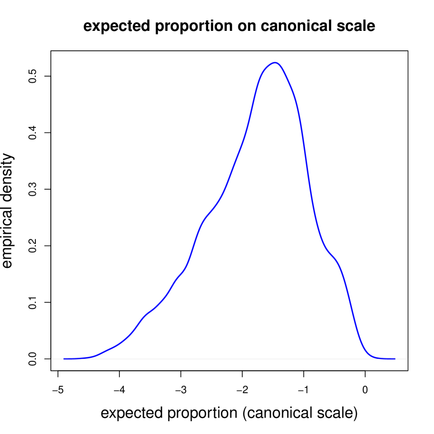
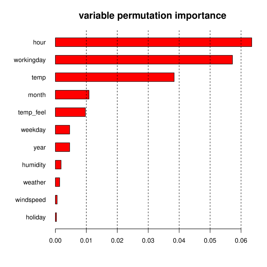
Figure 1: (lhs) Empirical density of canonical parameters $(\theta(\boldsymbol{x}_{i}))_{1\leq i\leq n}$, (rhs) variable permutation importance.

Figure 1 (lhs) shows the empirical density of the canonical parameters $\boldsymbol{x}_{i}\mapsto\theta(\boldsymbol{x}_{i})$ of the fitted model over our data $1\leq i\leq n$. We have negative skewness in this empirical density. A simple way of analyzing importance of feature components is to randomly permute one component $x_{j}$ at a time across all records $1\leq i\leq n$ and study the increase in objective function; this is the method of variable permutation importance introduced by [Breiman 2001]. We use as objective function the Bernoulli deviance loss which is proportional to the binary cross-entropy (also called log loss). Figure 1 (rhs) shows the variable permutation importances. There are three variables (hour, working day and temperature) that highly dominate the others. Note that variable permutation importance does not properly consider the dependence structure in $\boldsymbol{X}$, similarly to ICEs and PDPs, because permutation of $x_{j}$ is done without impacting $\boldsymbol{x}_{\setminus j}$.

6.2 1st and 2nd order contributions

The accuracy of the 2nd order contributions (6.2) will depend on the choice of the reference point $\boldsymbol{a}\in{\mathbb{R}}^{q}$. For network gradient descent fitting we have normalized the feature components to be centered and having unit variance, i.e. ${\mathbb{E}}_{P}[\boldsymbol{X}]=\boldsymbol{0}$ and ${\rm Var}_{P}(X_{j})=1$ for all $1\leq j\leq q$. This pre-processing is needed to efficiently apply stochastic gradient descent network fitting. We now translate these feature components by choosing a reference point $\boldsymbol{a}$ such that the objective function $G(\boldsymbol{a};\theta)$ is minimized, see (5). We use a plain vanilla gradient descent update (5.3) using a learning rate of $\varepsilon_{t+1}=10^{-2}/\|\nabla_{\boldsymbol{a}}G(\boldsymbol{a}^{(t)};\theta)\|$. For the quantile grid we choose $\alpha_{l}=l/100$ for $1\leq l\leq L=99$, thus, $\alpha\in\{1\%,\ldots,99\%\}$. The resulting decrease in objective function $G(\cdot;\theta)$ is plotted in Figure 2.

Figure 2: (lhs) Gradient descent for reference point $\boldsymbol{a}$, (rhs) 2nd order contributions (6.2).

Working with observed data, we need to discretize the MACQ analysis for quantile levels $\{\theta(\boldsymbol{X})=F_{\theta(\boldsymbol{X})}^{-1}(\alpha)\}$, $\alpha\in(0,1)$. We do this on a discrete grid by using a local smoother of degree 2, in particular, we use the R function locfit with parameters deg=2 and alpha=0.1 (being the chosen bandwidth) for observations $x^{\boldsymbol{a}}_{i,j}\theta_{j}(\boldsymbol{x}_{i})$ and $x^{\boldsymbol{a}}_{i,j}x^{\boldsymbol{a}}_{i,k}\theta_{j,k}(\boldsymbol{x}_{i})$, $1\leq i\leq n$, where we set $\boldsymbol{x}_{i}^{\boldsymbol{a}}=\boldsymbol{x}_{i}-\boldsymbol{a}$. We then fit the local smoother to these observations being ordered according to the ranks of $\theta(\boldsymbol{x}_{i})$, to work with the corresponding empirical output quantiles. Thus, for instance, the $\boldsymbol{a}$-adjusted 1st order attributions $S_{j}(\theta;\alpha_{l})$, $1\leq l\leq L$, are estimated empirically by using the pseudo code

$${\tt predict(locfit(}x^{\boldsymbol{a}}_{i,j}\theta_{j}(\boldsymbol{x}_{i})\sim{\rm rank}(\theta(\boldsymbol{x}_{i}))/n,{\tt alpha=0.1,deg=2),newdata=c(1:99)/100)}.$$

Figure 2 (rhs) gives the results after optimizing for the reference point $\boldsymbol{a}$. The orange color shows the 1st order contributions $C_{1}=\theta(\boldsymbol{a})+\sum_{j=1}^{q}S_{j}(\theta;\alpha)$, the cyan line shows the 2nd order contributions without interaction terms $C_{2}=\theta(\boldsymbol{a})+\sum_{j=1}^{q}(S_{j}(\theta;\alpha)-\frac{1}{2}T_{j,j}(\theta;\alpha))$ and the red line shows the full 2nd order contributions $C_{2,2}=\theta(\boldsymbol{a})+\sum_{j=1}^{q}(S_{j}(\theta;\alpha)-\frac{1}{2}T_{j,j}(\theta;\alpha))-\sum_{1\leq j<k\leq q}T_{j,k}(\theta;\alpha)$.

We observe from Figure 2 (rhs) that the full 2nd order contributions $C_{2,2}$ match the empirical quantiles (black dots) quite well which explains that there is a reference point $\boldsymbol{a}$ that allows for suitable 2nd order approximations over the entire quantile set. The shaded cyan area between $C_{2}$ (cyan line) and $C_{2,2}$ (red line) shows the influence of the interaction terms $T_{j,k}(\theta;\alpha)$, $j\neq k$, which illustrates that this model undergoes substantial interactions, and a simple generalized additive model (GAM) will not be able to model this data accurately.

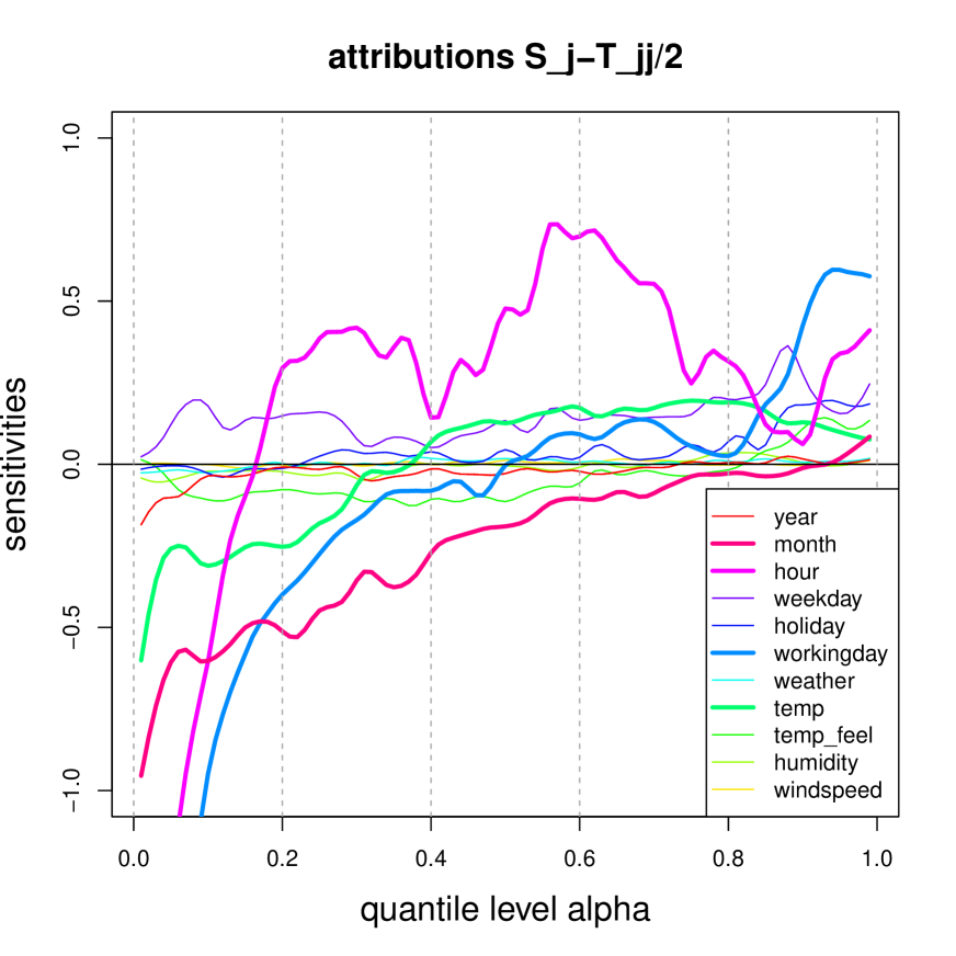
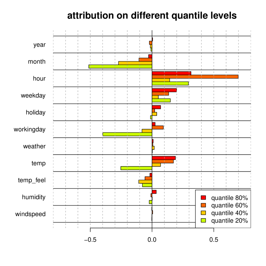
Figure 3: (lhs) attributions $S_{j}(\theta;\alpha)-\frac{1}{2}T_{j,j}(\theta;\alpha)$ excluding interaction terms, see (6.2), (rhs) attributions $S_{j}(\theta;\alpha)-\frac{1}{2}T_{j,j}(\theta;\alpha)$ for selected quantile levels $\alpha\in\{20\%,40\%,60\%,80\%\}$.

In Figure 3 (lhs) we show the attributions $S_{j}(\theta;\alpha)-\frac{1}{2}T_{j,j}(\theta;\alpha)$, excluding interaction terms $T_{j,k}(\theta;\alpha)$, $j\neq k$, relative to the optimal reference point $\boldsymbol{a}$. These attributions show the differences relative to canonical parameter in the reference point $\theta(\boldsymbol{a})$; when aggregating over $1\leq j\leq q$ this results in the cyan line of Figure 2 (rhs). Figure 3 (lhs) shows substantial sensitivities in the variables month, hour, working day and temperature. From this we conclude that these are the important variables in our regression model for differentiating the responses $Y$ w.r.t. available feature information $\boldsymbol{x}$. In contrast to the variable permutation importance plot of Figure 1 (rhs), this assessment correctly considers the dependence structure within the features $\boldsymbol{X}$. Moreover, this plot now allows us to analyze variable importance on different quantile levels by considering vertical slices in Figure 3 (lhs). We consider such vertical slices in Figure 3 (rhs) for four selected quantile levels $\alpha\in\{20\%,40\%,60\%,80\%\}$. We observe that the variables month, hour, workingday and temp undergo the biggest changes when moving from small quantiles to big ones. The quantile level at 20% can be explained by the three features temp, month and workingday, whereas for the quantile level at 60% has hour (daytime) as an important variable, see Figure 3 (rhs). Note that this is not the full picture, yet, as we do not consider interactions in these vertical slices; the importance of interactions is indicated by the cyan shaded area in Figure 2 (rhs) for different quantile levels.

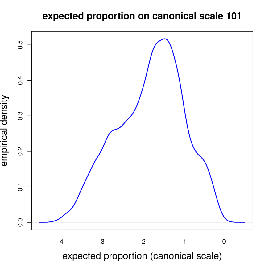
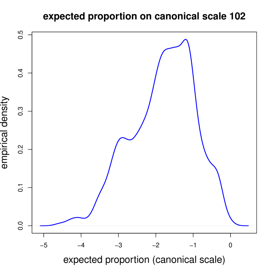
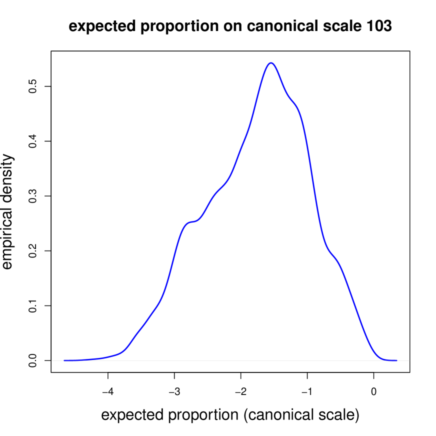
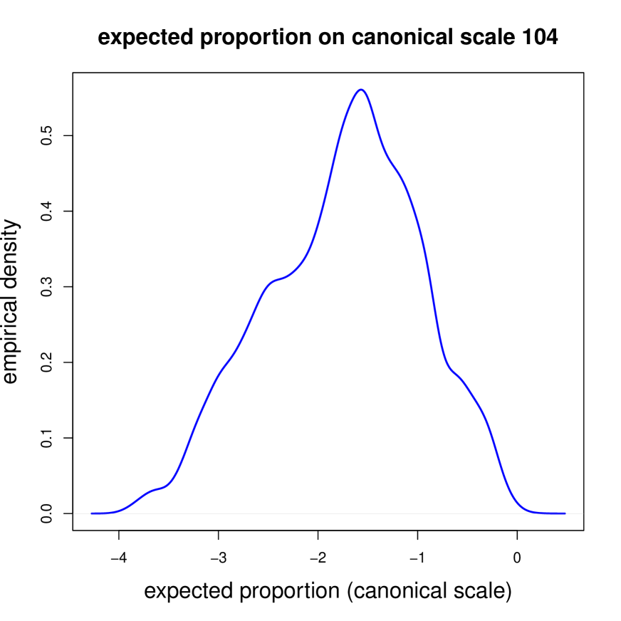
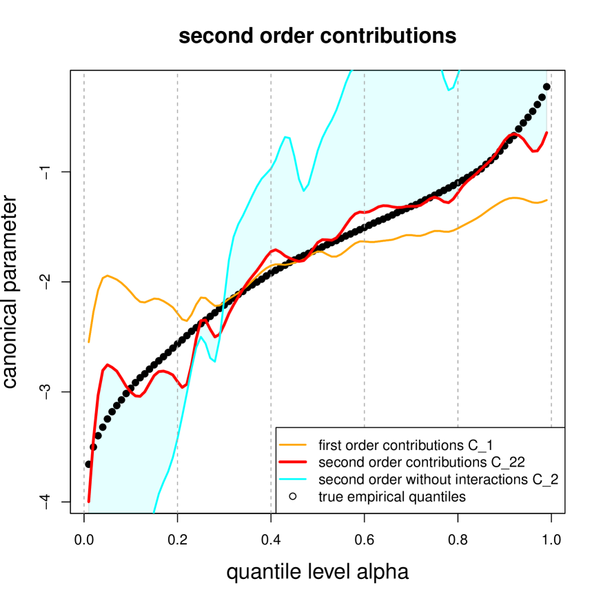
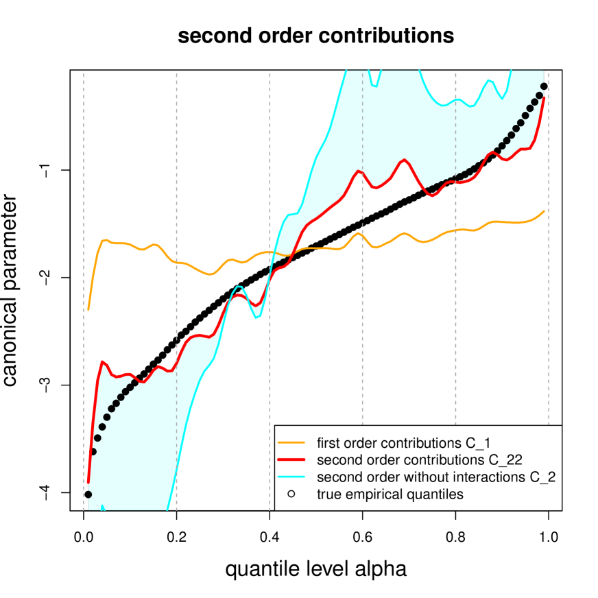
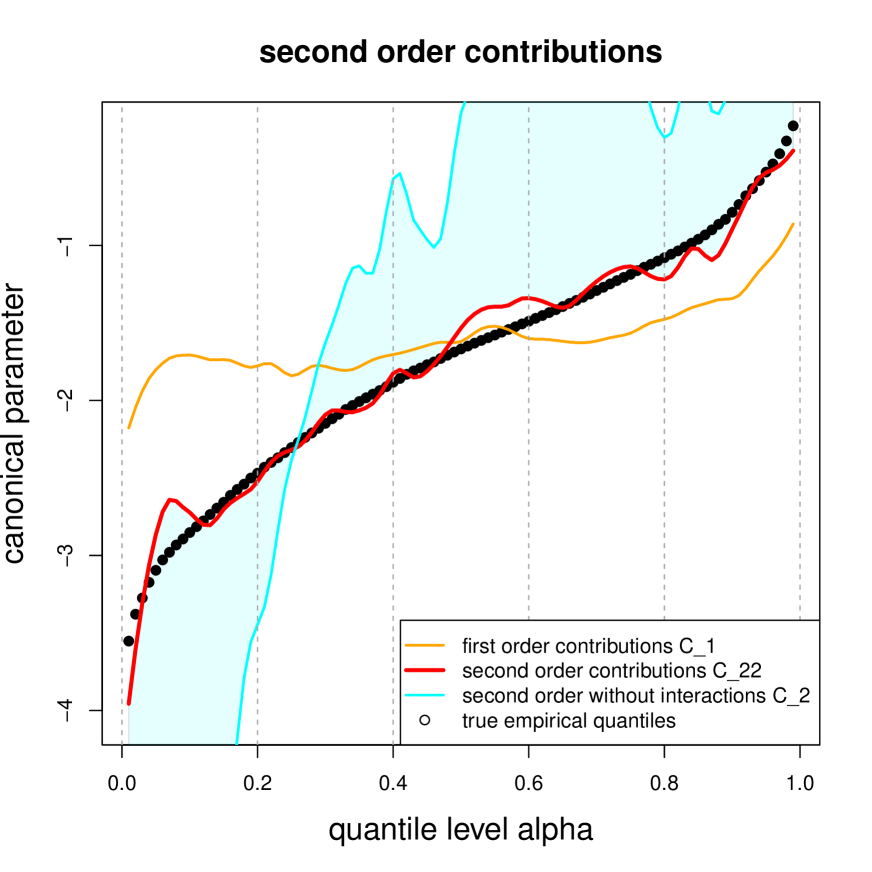
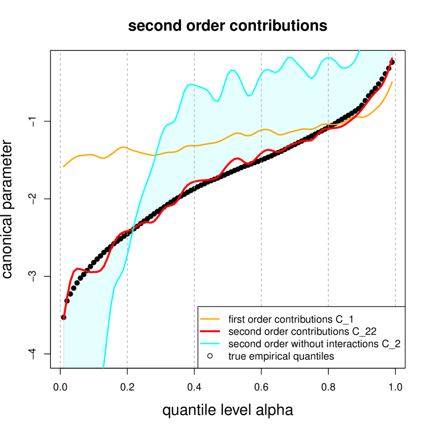
Figure 4: Robustness of 2nd order contributions across 4 different networks: (top row) empirical densities of canonical parameters $(\theta(\boldsymbol{x}_{i}))_{1\leq i\leq n}$, (bottom row) 2nd order contributions (6.2).

In Figure 4 we analyze the robustness of the attribution results. We do this by considering different networks $\boldsymbol{x}\mapsto\theta(\boldsymbol{x})$ for predicting the response variable $Y$. Network regression models lack a certain degree of robustness as gradient descent network fitting explores different (local) minima of the objective function; note that, in general, neural network fitting is not a convex minimization problem. This issue of non-uniqueness of good predictive models has been widely discussed in the literature, and ensembling may be one solution to mitigate this problem, we refer to [Dietterich 2000a, Dietterich 2000b], [Zhou et al. 2002], [Zhou 2012] and [Richman and Wüthrich 2020]. The top row shows the empirical distributions of the canonical parameters $(\theta(\boldsymbol{x}_{i}))_{1\leq i\leq n}$ for 4 different networks; we observe that there are some differences in these empirical densities. The bottom row shows the corresponding 2nd order contributions (6.2), split by 1st order contributions $C_{1}$, 2nd order contributions without interactions $C_{2}$ and the full 2nd order contributions $C_{2,2}$. At this level, we judge the attributions made to be rather robust over the different models, the general shapes of these graphs being similar, and also the interaction terms $C_{2,2}-C_{2}$ showing a similar structure and magnitude across the 4 different network models.

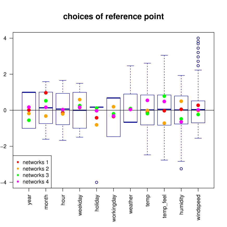
Figure 5: Choice of reference point $\boldsymbol{a}$ across 4 different networks illustrated for all feature components $1\leq j\leq q$.

From Figure 4 we also observe that the 1st order contributions $C_{1}$ intersect the quantiles $F_{\theta(\boldsymbol{X})}^{-1}(\alpha)$ at different levels for the 4 different calibrations. This indicates that the optimal reference point $\boldsymbol{a}$ is chosen differently in the different networks. Figure 5 shows the chosen reference points $\boldsymbol{a}$ in relation to the features $(\boldsymbol{x}_{i})_{1\leq i\leq n}$; as explained above, we have centered and normalized the feature components for gradient descent network fitting. The boxplots in Figure 5 show these centered and normalized features in comparison to the reference points of the 4 different networks. Some feature components have a very skewed distribution as can be seen from the thicker horizontal boxplot lines showing the median of each feature component $(x_{i,j})_{1\leq i\leq n}$, $1\leq j\leq q$. The reference point mostly lies within the interquartile range (IQR).

Remark 6.1

The feature components of $\boldsymbol{x}$ need pre-processing in order to be suitable for gradient descent fitting. Continuous and binary variables have been centered and normalized so that their gradients live in a similar range. This makes gradient descent fitting more efficient because all partial derivatives of the gradient are directly comparable. Our example does not have categorical feature components. Categorical feature components can be treated in different ways. For our MACQ proposal we envisage two different treatments. Firstly, dummy coding could be used. This requires the choice of a reference level, and considers all other levels relative to this reference level. The resulting marginal attributions should then be interpreted as differences to the reference level. Secondly, one can use embedding layers for categorical variables, see [Bengio et al. 2003] and [Guo and Berkhahn 2016]. In that case the attribution analysis can directly be done on these learned embeddings of categorical levels, in complete analogy to the continuous variables.

6.3 Attribution to individual instances

Next, we focus on individual instances $\boldsymbol{x}^{\boldsymbol{a}}_{i}=\boldsymbol{x}_{i}-\boldsymbol{a}$ and study individual marginal contributions $\omega_{i,j}=(x_{i,j}-a_{j})\theta_{j}(\boldsymbol{x}_{i})-(x_{i,j}-a_{j})^{2}\theta_{j,j}(\boldsymbol{x}_{i})/2$ to attribution $S_{j}(\theta;\alpha)-T_{j,j}(\theta;\alpha)/2$.

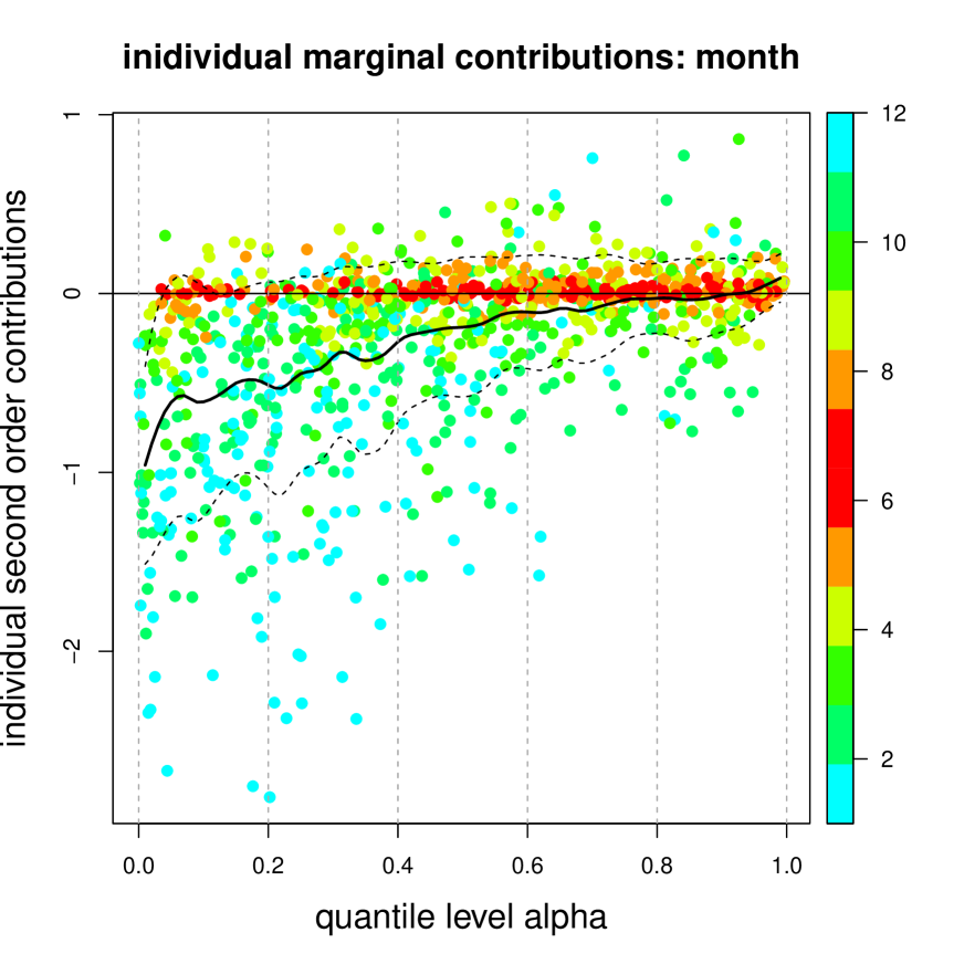
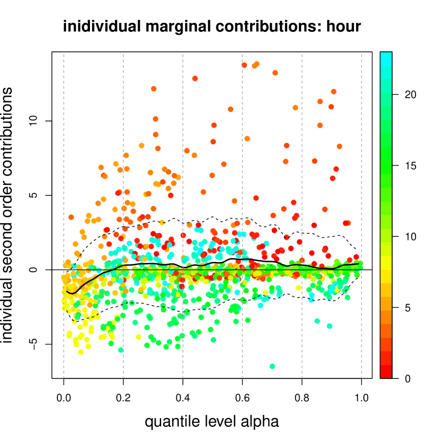
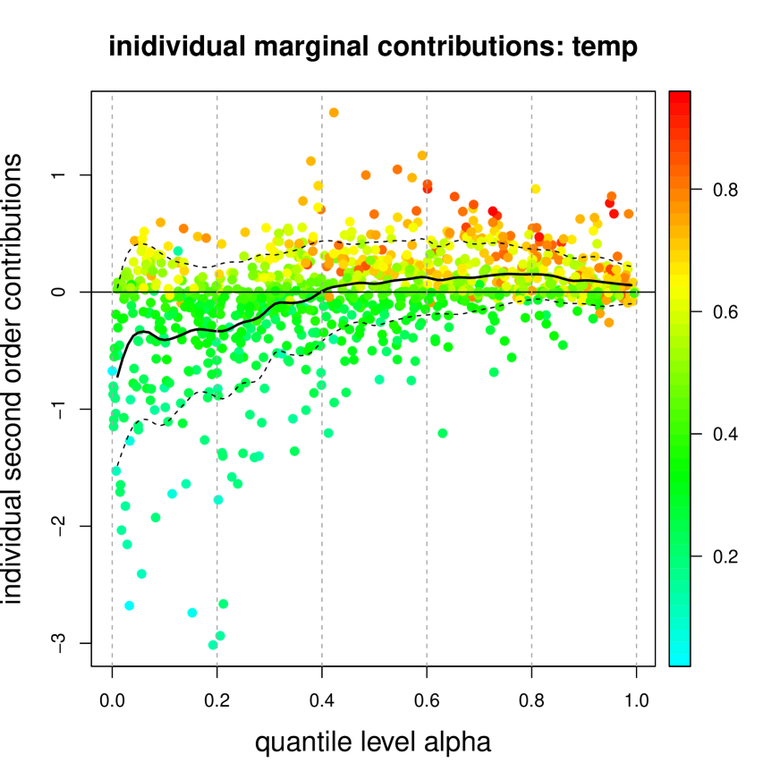
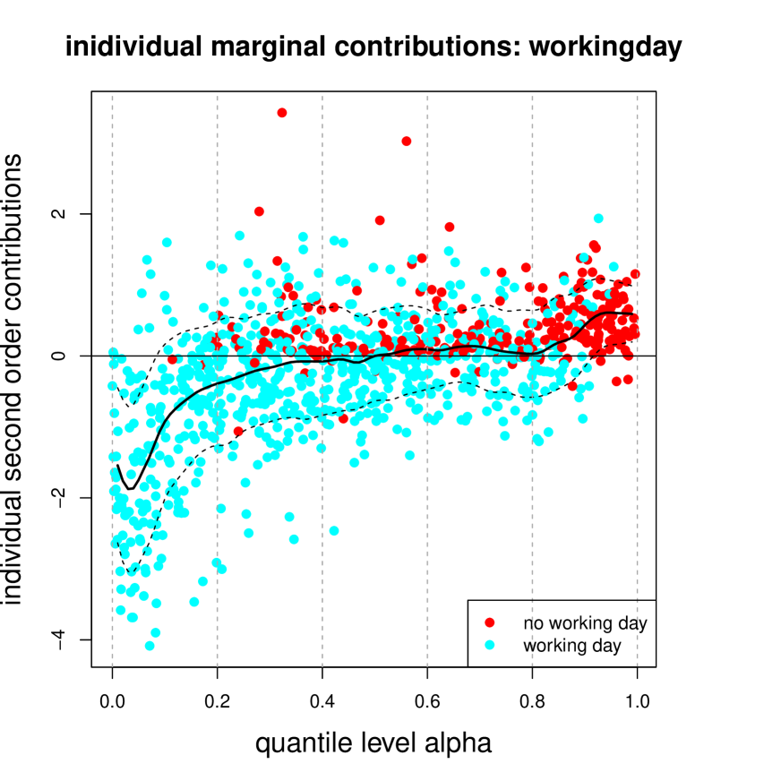
Figure 6: Individual marginal contributions $\omega_{i,j}$ of 1,000 randomly selected instances $\boldsymbol{x}_{i}$ for (top-left) $j={\tt month}$, (top-right) $j={\tt hour}$, (bottom-left) $j={\tt temp}$ and (bottom-right) $j={\tt workingday}$; the black line shows attribution $S_{j}(\theta;\alpha)-T_{j,j}(\theta;\alpha)/2$ and the black dotted line gives one standard deviation; the $y$-scales differs in the plots and the colors illustrate the feature values $x_{j}$.

For Figure 6 we select at random 1,000 different instances, and plot their individual marginal contributions $\omega_{i,j}$ to the attributions $S_{j}(\theta;\alpha)-T_{j,j}(\theta;\alpha)/2$ (black solid line). The ordering on the $x$-axis for the selected instances $\boldsymbol{x}_{i}$ is obtained by considering the empirical quantiles of the responses $\theta(\boldsymbol{x}_{k})$ over all instances $1\leq k\leq n$. We start with Figure 6 (bottom-right) which shows the binary variable workingday. This variable clearly differentiates low from high quantiles $F_{\theta(\boldsymbol{X})}^{-1}(\alpha)$, showing that the casual rental proportion $Y$ is in average bigger for non-working days (red dots). Moreover, for low quantiles levels the working day variable clearly lowers (expected response) $\theta(\boldsymbol{x})$ compared to the reference level $\theta(\boldsymbol{a})$, as the cyan dots are below the horizontal black line at 0 which corresponds to the reference level. In addition to the average attributions $S_{j}(\theta;\alpha)-T_{j,j}(\theta;\alpha)/2$ (black solid line), the plot is complemented by black dotted lines giving one (empirical) standard deviation

$${\rm Var}_{P}\left((X_{j}-a_{j})\theta_{j}(\boldsymbol{X})-(X_{j}-a_{j})^{2}\theta_{j,j}(\boldsymbol{X})/2\left|\theta(\boldsymbol{X})=F_{\theta(\boldsymbol{X})}^{-1}(\alpha)\right.\right)^{1/2}.$$

The sizes of these standard deviations quantify the heterogeneity in the individual marginal contributions $\omega_{i,j}$. This can either be because of heterogeneity of the portfolio $x_{i,j}$ on a certain quantile level, or because we have a rough regression surface implying heterogeneity in derivatives $\theta_{j}(\boldsymbol{x}_{i})$ and $\theta_{j,j}(\boldsymbol{x}_{i})$.

Next, we study the variable temp of Figure 6 (bottom-left). In this plot we see a clear positive dependence between quantile levels and temperature, showing that casual rentals are generally low for low temperatures, which can either be the calendar season or bad weather conditions. We have clearly more heterogeneity in features (and resulting derivatives $\theta_{j}(\boldsymbol{x}_{i})$ and $\theta_{j,j}(\boldsymbol{x}_{i})$) contributing to low quantile levels than to higher ones. The variable temp is highly correlated with calendar month, and the calendar month plot in Figure 6 (top-left) looks similar, saying that casual rental proportions $Y$ are negatively impacted by winter seasons. There are some low proportions, though, also for summer months, these need to be explained by other variables, e.g., they may correspond to a rainy day or to a specific daytime. The interpretation of the variable hour in Figure 6 (top-right) is slightly more complicated since we do not have monotonicity of $\theta(\boldsymbol{x})$ in this variable, see also Figure 12. Nevertheless we also see a separation between working and leisure times (for the time-being ignoring interactions with holidays and weekends).

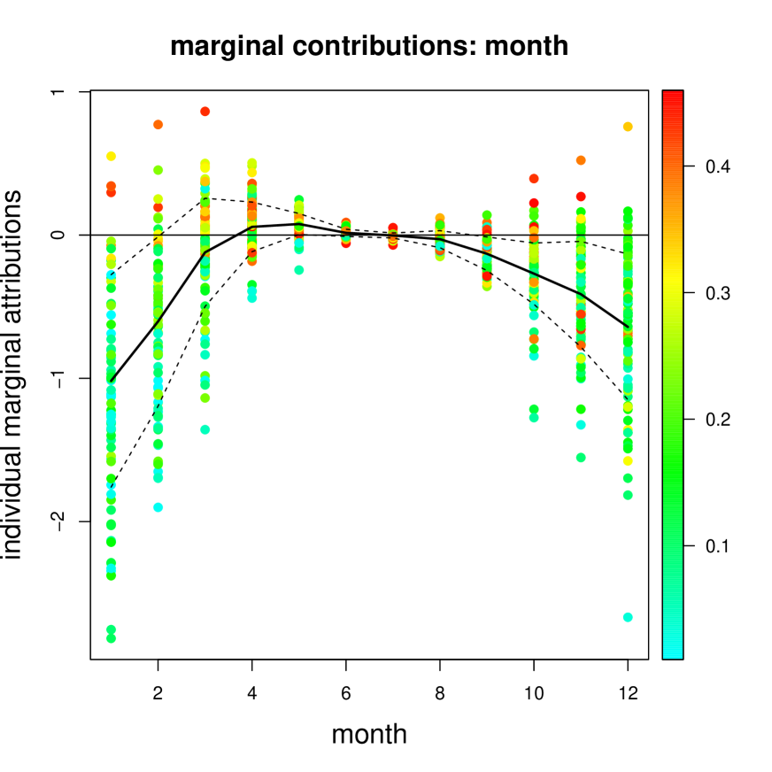
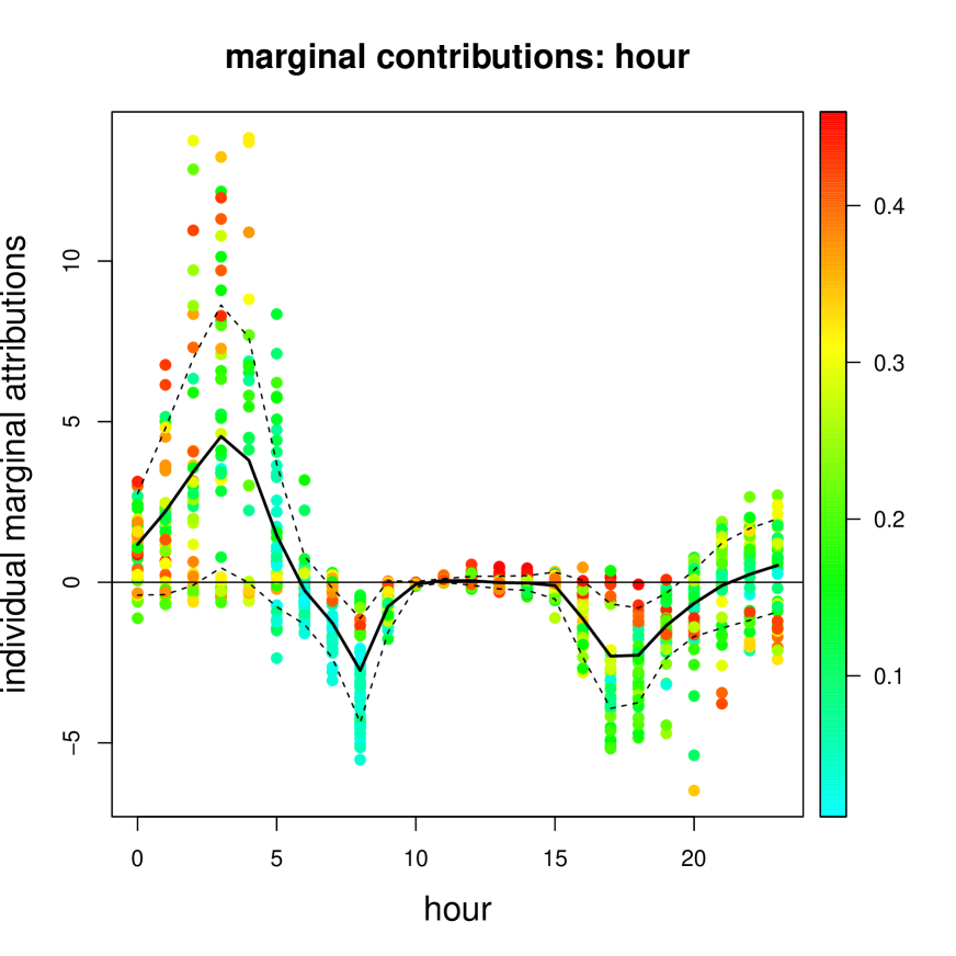
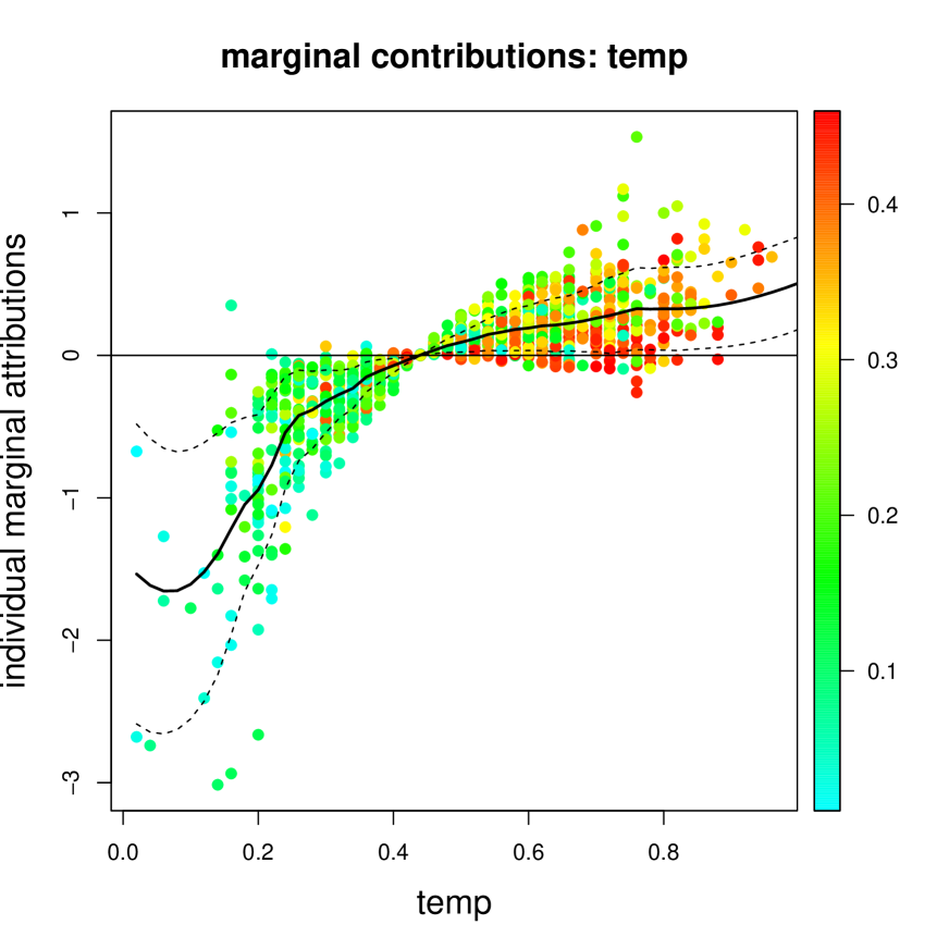
Figure 7: Individual marginal contribuions $\omega_{i,j}$ of 1,000 randomly selected instances $\boldsymbol{x}_{i}$ for (lhs) $j={\tt month}$, (middle) $j={\tt hour}$ and (rhs) $j={\tt temp}$; the black line shows the empirical average; the colors show the expected responses $\mu(\boldsymbol{x}_{i})\in(0,1)$ (casual rental proportions).

In Figure 6 we have plotted the individual marginal contributions $\omega_{i,j}$ on the $y$-axis against the quantiles $\alpha\in(0,1)$ on the $x$-axis to explain how the features $\boldsymbol{x}_{i}$ enter the quantile levels $F_{\theta(\boldsymbol{X})}^{-1}(\alpha)$. This is the 3-ways analysis mentioned above, where the third dimension is highlighted by using different colors in Figure 6. Alternatively, we can also try to understand how this third dimension of different feature values $x_{j}$ contributes to the individual marginal contributions $\omega_{i,j}$. Figure 7 plots the individual marginal contributions $\omega_{i,j}$ on the $y$-axis against the feature values $x_{j}$ on the $x$-axis. The black line shows the averages of $\omega_{i,j}$ over all instances, and the colored dots show the 1,000 randomly selected instances $\boldsymbol{x}_{i}$ with the colors illustrating the expected responses, i.e. the expected casual rental proportions $\mu(\boldsymbol{x}_{i})=\sigma(\theta(\boldsymbol{x}_{i}))\in(0,1)$. The general shape of the black lines in these graphs reflects well the marginal empirical observations in Figure 12. However, the detailed structure slightly differs in these plots as they do not exactly show the same quantity, the latter shows a marginal empirical graph, whereas Figure 7 quantifies individual marginal contributions to expected responses $\theta(\boldsymbol{x})$ in an additive way (on the canonical scale). Figure 7 (rhs) shows a clear monotone plot which also results in a separation of the colors, whereas the colors in Figure 7 (lhs, middle) can only be fully understood by also studying contributions and interactions with other components $x_{i,k}$, $k\neq j$.

6.4 Interaction terms

There remains the analysis of the interaction terms $-T_{j,k}(\theta;\alpha)$, $j\neq k$, that account for the cyan shaded are in Figure 2 (rhs). These interaction terms are shown in Figure 8.

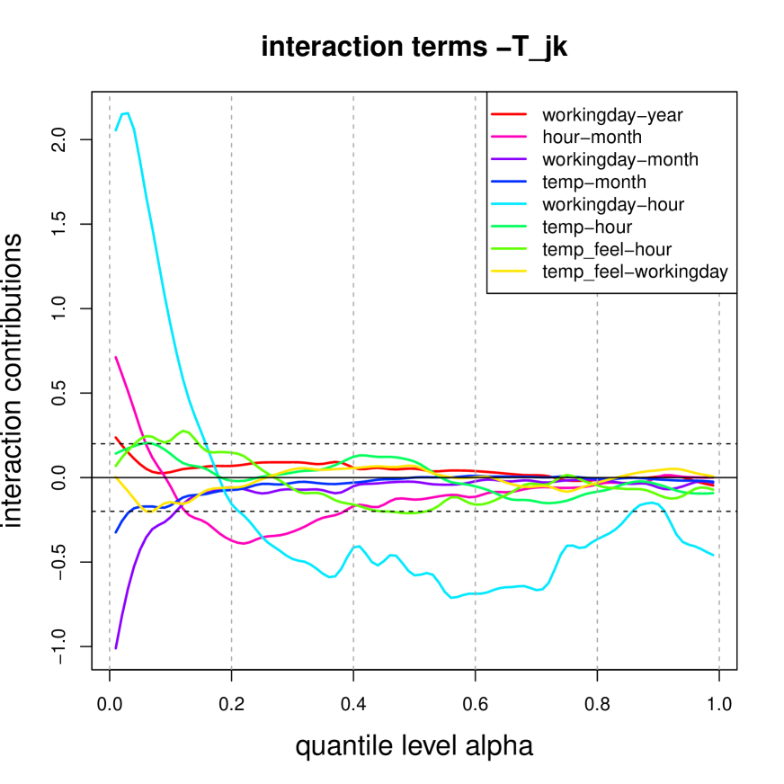
Figure 8: Off-diagonal terms $-T_{j,k}(\theta;\alpha)$ giving the interactions.

To not overload Figure 8 we only show the interaction terms $T_{j,k}$ for which $\max_{\alpha}|T_{j,k}(\theta;\alpha)|>0.2$. We identify three major interaction terms: workingday-hour, workingday-month and hour-month. Of course, these interactions make perfect sense in describing the casual rental proportion. For small quantiles also interactions temp-month and temp-hour are important. Interestingly, we also find an interaction workingday-year: in the data there is a positive trend of registered rental bike users (in absolute terms) which interacts differently on working and non-working days because casual rentals are more frequent on non-working days. Identifying the importance of these interactions highlights that it will not be sufficient to work within a generalized linear model (GLM) or a generalized additive model (GAM) unless we add explicit interaction terms to them.

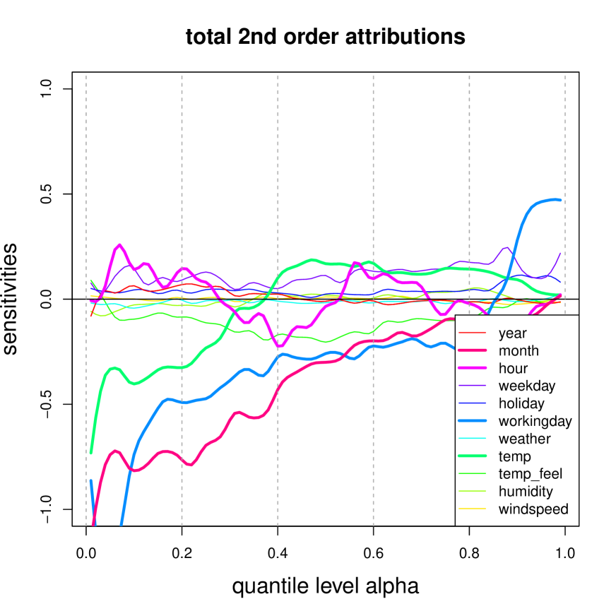
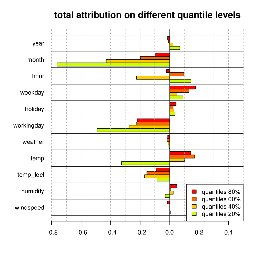
Figure 9: (lhs) 2nd order attributions $V_{j}(\theta;\alpha)$ including interaction terms, and (rhs) $V_{j}(\theta;\alpha)$ for selected quantile levels $\alpha\in\{20\%,40\%,60\%,80\%\}$.

In the final step we combine the attributions $S_{j}(\theta;\alpha)-T_{j,j}(\theta;\alpha)/2$ with the interaction terms $T_{j,k}(\theta;\alpha)$, $k\leq j$. A natural way is to just allocate half of the interaction terms $T_{j,k}(\theta;\alpha)$ to each component $j$ and $k$. This then provides allocated 2nd order attribution to components $1\leq j\leq q$

$$V_{j}(\theta;\alpha)~{}=~{}S_{j}(\theta;\alpha)-T_{j,j}(\theta;\alpha)/2-\sum_{j\neq k}T_{j,k}(\theta;\alpha)/2~{}=~{}S_{j}(\theta;\alpha)-\sum_{k=1}^{q}T_{j,k}(\theta;\alpha)/2.$$

Adding the reference level $\theta(\boldsymbol{a})$, we again receive the full 2nd order contributions $C_{2,2}=\theta(\boldsymbol{a})+\sum_{j=1}^{q}V_{j}(\theta;\alpha)$ illustrated by the red line in Figure 2 (rhs). In Figure 9 we provide these attributions $V_{j}(\theta;\alpha)$ for quantiles $\alpha\in(0,1)$. These plots differ from Figure 3 only by the inclusion of the 2nd order off-diagonal (interaction) terms. Comparing the right-hand sides of these two plots we observe that firstly the level is shifted, which is explained by the shaded cyan area in Figure 2 (rhs). Secondly, interactions impact mainly the small quantiles in our example, this is clear from Figure 8 and, for instance, impacts the significance of hour on the 20% quantile level.

6.5 Scrolling through the network layers

Up to this point our MACQ analysis has been fully general, in the sense that it can be applied to any smooth deep learning model. In the last step of our analysis we specifically focus on the deep network introduced in Section 6.1, and we try to better understand how networks learn new representations through the network layers. A deep feed-forward neural network $\theta:{\mathbb{R}}^{q}\to{\mathbb{R}}$ is a composition of $d$ hidden neural network layers $\boldsymbol{z}^{(k)}:{\mathbb{R}}^{q_{k-1}}\to{\mathbb{R}}^{q_{k}}$, $1\leq k\leq d$; we initialize input dimension $q_{0}=q$. Define the composition $\boldsymbol{x}\mapsto\boldsymbol{z}^{(d:1)}(\boldsymbol{x})=(\boldsymbol{z}^{(d)}\circ\ldots\circ\boldsymbol{z}^{(1)})(\boldsymbol{x})$ which maps input $\boldsymbol{x}\in{\mathbb{R}}^{q}$ to the last hidden network layer having dimension $q_{d}$. Network (6.1) with logistic output can then be written as

$$\boldsymbol{x}\in{\mathbb{R}}^{q}~{}~{}\mapsto~{}~{}\mu(\boldsymbol{x})=\sigma(\theta(\boldsymbol{x}))=\sigma\left(\beta_{0}+\boldsymbol{\beta}^{\top}\boldsymbol{z}^{(d:1)}(\boldsymbol{x})\right),$$

with bias/intercept $\beta_{0}\in{\mathbb{R}}$ and regression parameter/weight $\boldsymbol{\beta}\in{\mathbb{R}}^{q_{d}}$. This should be compared to linear regression (3.4).

Each hidden layer learns a new representation of the inputs $\boldsymbol{x}_{i}$, that is, the representations learned in layer $k$ are given by $\boldsymbol{x}^{(k:1)}_{i}:=(\boldsymbol{z}^{(k)}\circ\ldots\circ\boldsymbol{z}^{(1)})(\boldsymbol{x}_{i})$, for $1\leq i\leq n$. We can view these learned representations as new inputs to the remaining network after hidden layer $k$

$$\boldsymbol{x}\in{\mathbb{R}}^{q_{k}}~{}~{}\mapsto~{}~{}\sigma\left(\beta_{0}+\boldsymbol{\beta}^{\top}\boldsymbol{z}^{(d:k+1)}(\boldsymbol{x})\right)=\sigma\left(\beta_{0}+\boldsymbol{\beta}^{\top}(\boldsymbol{z}^{(d)}\circ\ldots\circ\boldsymbol{z}^{(k+1)})(\boldsymbol{x})\right).$$

In the following analysis we consider the instances $(Y_{i},\boldsymbol{x}^{(k:1)}_{i})$ with these learned features $\boldsymbol{x}^{(k:1)}_{i}$ as inputs to the remaining network $\boldsymbol{z}^{(d:k+1)}$ after layer $k$, and we perform the same MACQ analysis in this reduced setup.

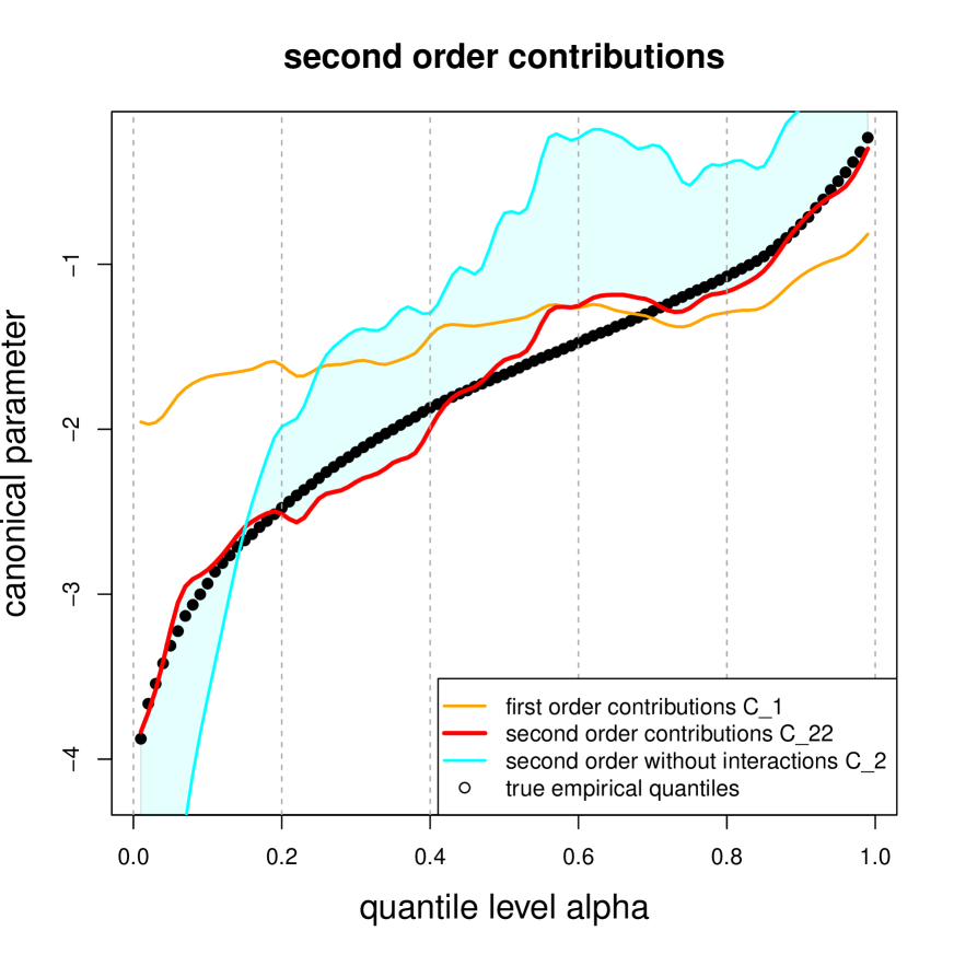
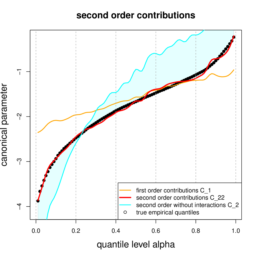
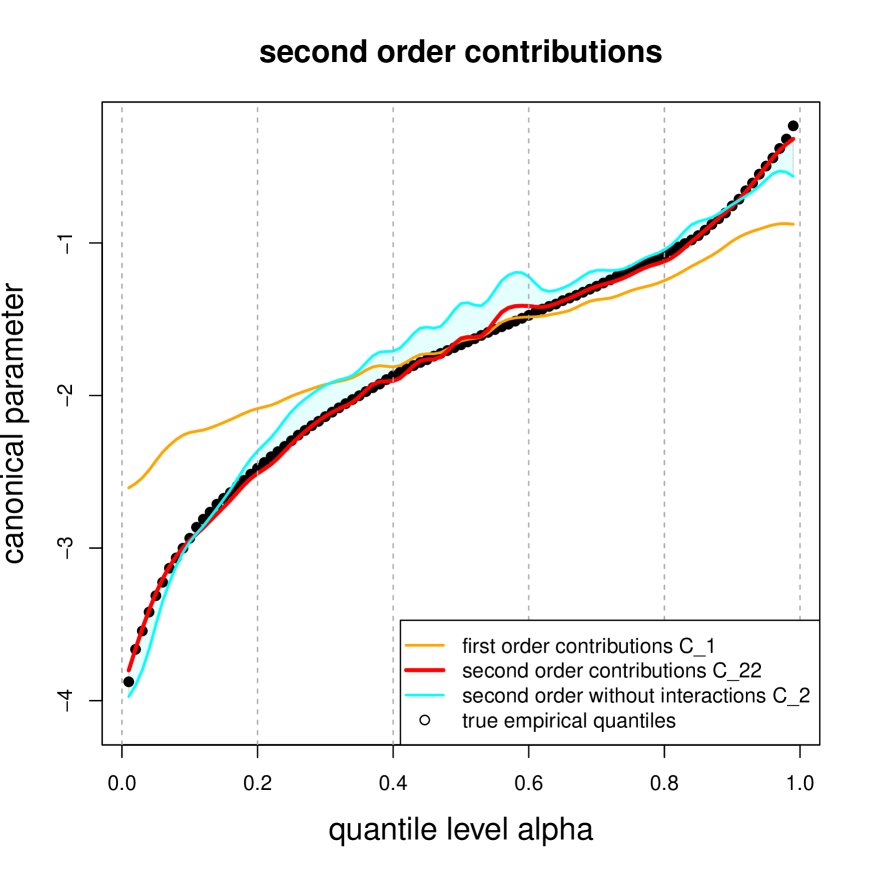
Figure 10: 2nd order contributions (6.2) of the (learned) representations: (lhs) original inputs $\boldsymbol{x}_{i}$, (middle) learned representations $\boldsymbol{x}^{(1:1)}_{i}$, and (rhs) learned representations $\boldsymbol{x}^{(2:1)}_{i}$.

Figure 10 provides the 2nd order contributions (6.2) of the original inputs (lhs), the learned representations $\boldsymbol{x}^{(1:1)}_{i}$ in the first hidden layer (middle), and the learned representations $\boldsymbol{x}^{(2:1)}_{i}$ in the second hidden layer (rhs) on the corresponding remaining networks $\boldsymbol{z}^{(3:k+1)}$. We interpret these MACQ results as follows. The first hidden layer (middle graph) has mainly a smoothing effect in recomposing the inputs $\boldsymbol{x}_{i}$ suitably. The second layer takes care of the interaction effects diminishing the cyan shaded area in Figure 10 (rhs). Of course, this makes perfect sense as the output layer considers a linear function with weight $\boldsymbol{\beta}\in{\mathbb{R}}^{q_{d}}$ which no longer allows for interactions. Therefore, interactions need to be learned in the previous layers. The same applies to non-linear structures (on the canonical scale). This completes our example.

7 Conclusions

This manuscript proposes a novel gradient-based global model-agnostic tool that can be calculated efficiently for differentiable deep learning models and produces informative visualizations. This tool studies marginal attribution to feature components on a given response level. Marginal attributions allow us to separate marginal effects of individual feature components from interaction effects, and they allow us to study resulting variable importance plots on different parts of the decision space characterized by different response levels. This variable importance is measured w.r.t. a reference point that calibrates the entire space for our explanation. Finding a good reference point has been efficiently performed by a simple gradient descent search. A main result of our model-agnostic tool is a 3-way relationship between marginal attribution, output level and feature value which can be illustrated in different ways. This extends response sensitivity analyses, such as accumulated local effects, by an additional marginal attribution view.

Appendix A Sensitivities in distortion risk measures

The purpose of this appendix is to briefly explain distortion risk measures and how they relate to marginal attribution. For this discussion we impose stronger assumptions than we need above, i.e., these more restrictive assumptions are only made for the explanation here. Assume the expected response $\mu(\boldsymbol{X})$ has a continuous distribution function $F_{\mu(\boldsymbol{X})}$. It follows that $U_{\mu(\boldsymbol{X})}=F_{\mu(\boldsymbol{X})}(\mu(\boldsymbol{X}))$ is uniformly distributed on $[0,1]$. Choose a density $\zeta$ on $[0,1]$. We can interpret $\zeta(U_{\mu(\boldsymbol{X})})$ as a probability distortion (probability re-weighting scheme inducing a change of probability measure) because we have

$${\mathbb{E}}_{P}\left[\zeta(U_{\mu(\boldsymbol{X})})\right]=\int_{0}^{1}\zeta(u)du=1.$$

The distorted expected response can then be defined by

$$\varrho(\mu(\boldsymbol{X});\zeta)={\mathbb{E}}_{P}\left[\mu(\boldsymbol{X})\zeta(U_{\mu(\boldsymbol{X})})\right].$$

The functional $\varrho(\mu(\boldsymbol{X});\zeta)$ describes a distortion risk measure, see [Wang 1996] and [Acerci 2002]. It can be interpreted as a Radon–Nikodým derivative changed probability measure $dP_{\zeta}(\boldsymbol{X}=\boldsymbol{x})=\zeta(U_{\mu(\boldsymbol{x})})dP(\boldsymbol{X}=\boldsymbol{x})$. We study the sensitivities of this distortion risk measure w.r.t. the components of $\boldsymbol{X}$. Assume that the following directional derivatives exist in zero for all $1\leq j\leq q$

$$S_{j}(\mu;\zeta)=\frac{\partial}{\partial\varepsilon}\left.\varrho\left(\mu\left((X_{1},\ldots,X_{j-1},X_{j}(1+\varepsilon),X_{j+1},\ldots X_{q})^{\top}\right);\zeta\right)\right|_{\varepsilon=0}.$$

Then, $S_{j}(\mu;\zeta)$ can be interpreted as the sensitivity of $\boldsymbol{X}\mapsto\mu(\boldsymbol{X})$ in feature component $X_{j}$. [Hong 2009] and [Tsanakas and Millossovich 2015] prove under different sets of assumptions that these sensitivities satisfy

$$S_{j}(\mu;\zeta)={\mathbb{E}}_{P}\left[X_{j}\mu_{j}(\boldsymbol{X})\zeta(U_{\mu(\boldsymbol{X})})\right].$$

Observe that this exactly uses the marginal attribution (2.6). We still have the freedom of choosing the density $\zeta$ on $[0,1]$. If we choose the uniform distribution $\zeta\equiv 1$ on $[0,1]$ we receive the average expected response and its average marginal attribution

$$\varrho(\mu(\boldsymbol{X});\zeta\equiv 1)={\mathbb{E}}_{P}[\mu(\boldsymbol{X})]\qquad\text{ and }\qquad S_{j}(\mu;\zeta\equiv 1)={\mathbb{E}}_{P}[X_{j}\mu_{j}(\boldsymbol{X})].$$

If we choose for density $\zeta$ the Dirac measure $\delta_{\alpha}$ in $\alpha\in(0,1)$, which allocates probability weight 1 to $\alpha$, this gives us the $\alpha$-quantile

$$\varrho(\mu(\boldsymbol{X});\zeta=\delta_{\alpha})=F_{\mu(\boldsymbol{X})}^{-1}(\alpha).$$

For its sensitivities we receive for $1\leq j\leq q$

$$S_{j}(\mu;\zeta=\delta_{\alpha})~{}=~{}{\mathbb{E}}_{P}\left[X_{j}\mu_{j}(\boldsymbol{X})\left|\mu(\boldsymbol{X})=F_{\mu(\boldsymbol{X})}^{-1}(\alpha)\right.\right],$$

which exactly corresponds to 1st order attribution (3.1).

Remark. We could choose any other density $\zeta$ on $[0,1]$ to obtain sensitivities of other distortion risk measures. Such other choices may also have interesting counterparts in interpreting smooth deep learning models, by reflecting attention to different areas of the prediction space.

Appendix B Descriptive analysis of bike rental example

In this appendix, we give a brief descriptive analysis of the data used that helps us to interpret the network regression models. The data comprises the number of casual and registered bike rentals every hour from 2011/01/01 until 2012/12/31. This data has originally been studied in [Fanaee-T and Gama 2014] and [Apley and Zhu 2020], and it can be downloaded from https://archive.ics.uci.edu/ml/datasets/Bike+Sharing+Dataset. Listing 1 gives a short excerpt of the data.

Listing 1: Excerpt of bike rental data.

⬇

1’data.frame’: 17379 obs. of 13 variables:

2 $ date : Date, format: "2011-01-01" "2011-01-01" "2011-01-01" ...

3 $ year : num 2011 2011 2011 2011 2011 ...

4 $ month : int 1 1 1 1 1 1 1 1 1 1 ...

5 $ hour : int 0 1 2 3 4 5 6 7 8 9 ...

6 $ weekday : int 6 6 6 6 6 6 6 6 6 6 ...

7 $ holiday : Factor w/ 2 levels "holiday","no-holiday": 2 2 2 2 2 2 2 2 2 2 ...

8 $ workingday: Factor w/ 2 levels "no-working","workingday": 1 1 1 1 1 1 1 1 1 1 ...

9 $ weather : num 1 1 1 1 1 2 1 1 1 1 ...

10 $ temp : num 0.24 0.22 0.22 0.24 0.24 0.24 0.22 0.2 0.24 0.32 ...

11 $ temp_feel : num 0.288 0.273 0.273 0.288 0.288 ...

12 $ humidity : num 0.81 0.8 0.8 0.75 0.75 0.75 0.8 0.86 0.75 0.76 ...

13 $ windspeed : num 0 0 0 0 0 0.0896 0 0 0 0 ...

14 $ casual : int 3 8 5 3 0 0 2 1 1 8 ...

15 $ registered: int 13 32 27 10 1 1 0 2 7 6 ...

16 $ count : int 16 40 32 13 1 1 2 3 8 14 ...

As response variable we consider the proportion of casual rentals relative to all rentals, thus, we set response $Y={\tt casual}/{\tt count}\in[0,1]$ on an hourly grid over the entire observation period. These are $n=17,379$ hours from 2011/01/01 until 2012/12/31, see line 1 of Listing 1. We note that ${\tt count}\geq 1$ for all observations, which makes $Y$ well-defined throughout the whole observation period. The goal is to predict this response variable $Y$ based on available feature information $\boldsymbol{x}$ which is provided on lines 3-13 of Listing 1. These are the year, month and hour of the observations $Y$. The weekday (with 0 for Sunday), holiday (yes/no for public holiday), workingday (yes/no, the former neither being a public holiday nor a weekend), weather (1,2 and 3 for clear, cloudy and rain/snow), temperature temp, the felt temperature temp_feel, humidity and windspeed. Note that all these features are continuous or binary, thus, we can directly use this feature encoding for regression modeling.

We illustrate this data. Figure 11 shows the observed responses $Y={\tt casual}/{\tt count}$ over the entire observation period. In average the casual rentals make 17% of all rentals, and the empirical density of $Y$ is strongly skewed.

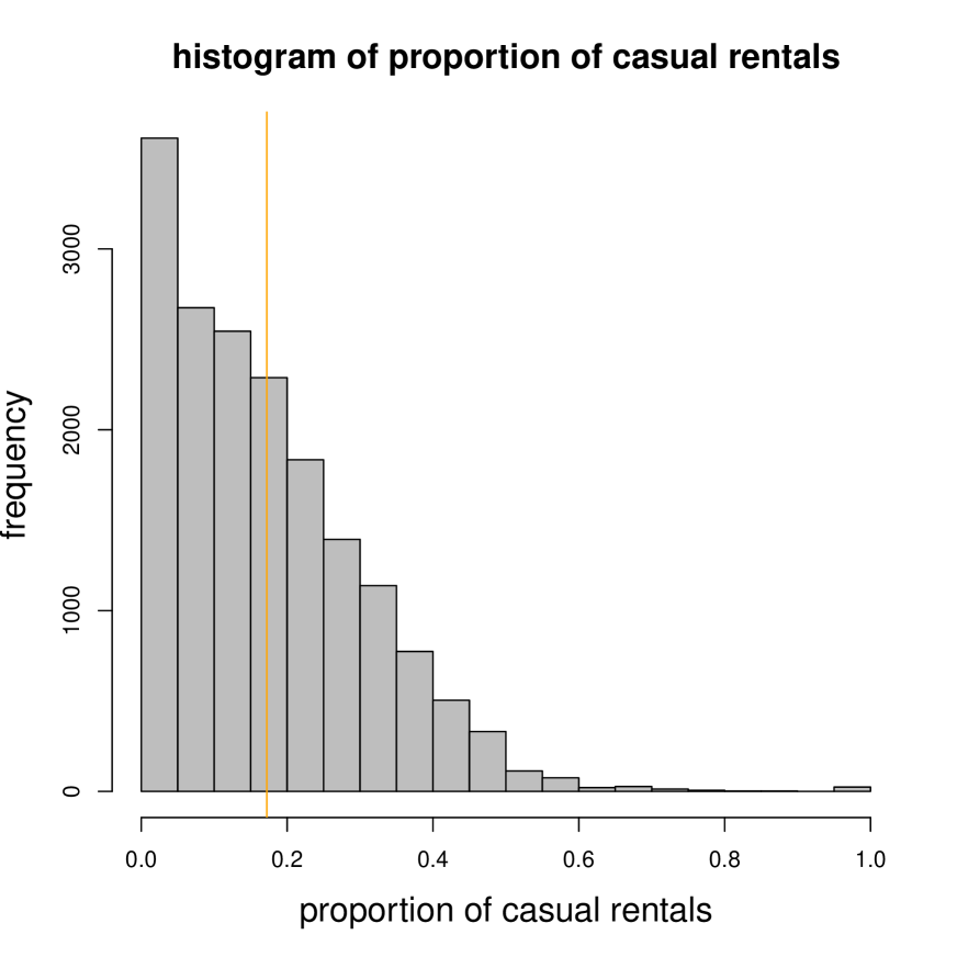
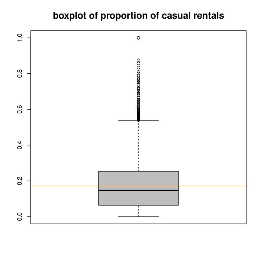
Figure 11: (lhs) Histogram and (rhs) boxplot of (hourly) responses $Y={\tt casual}/{\tt count}\in[0,1]$ over the entire observation period; the orange line shows the empirical mean of 17%.

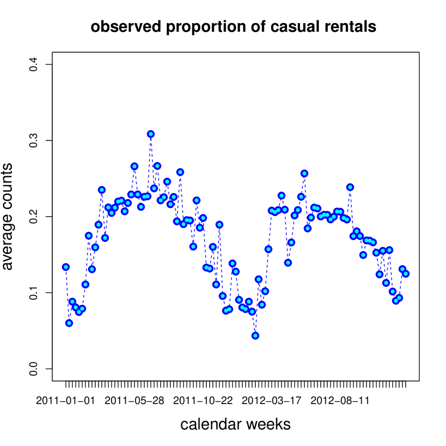
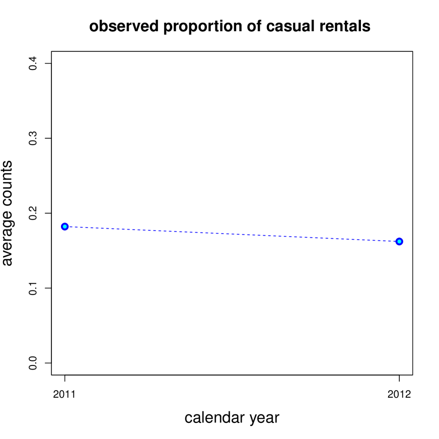
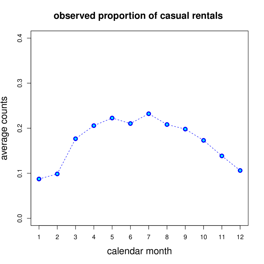
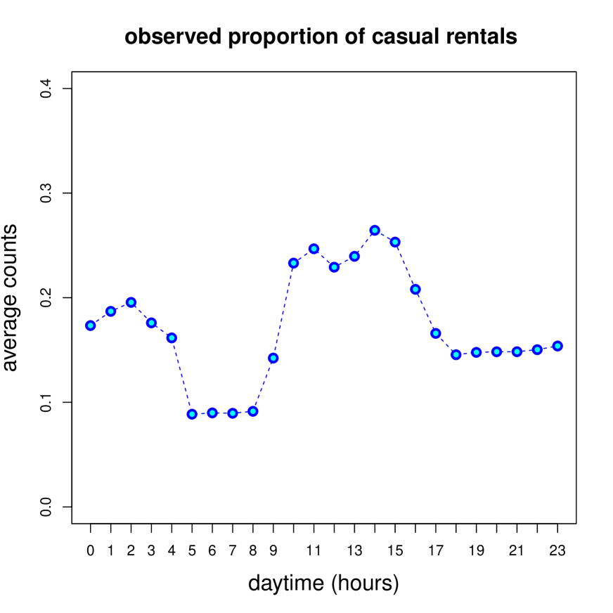
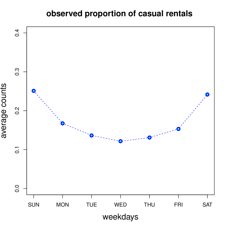
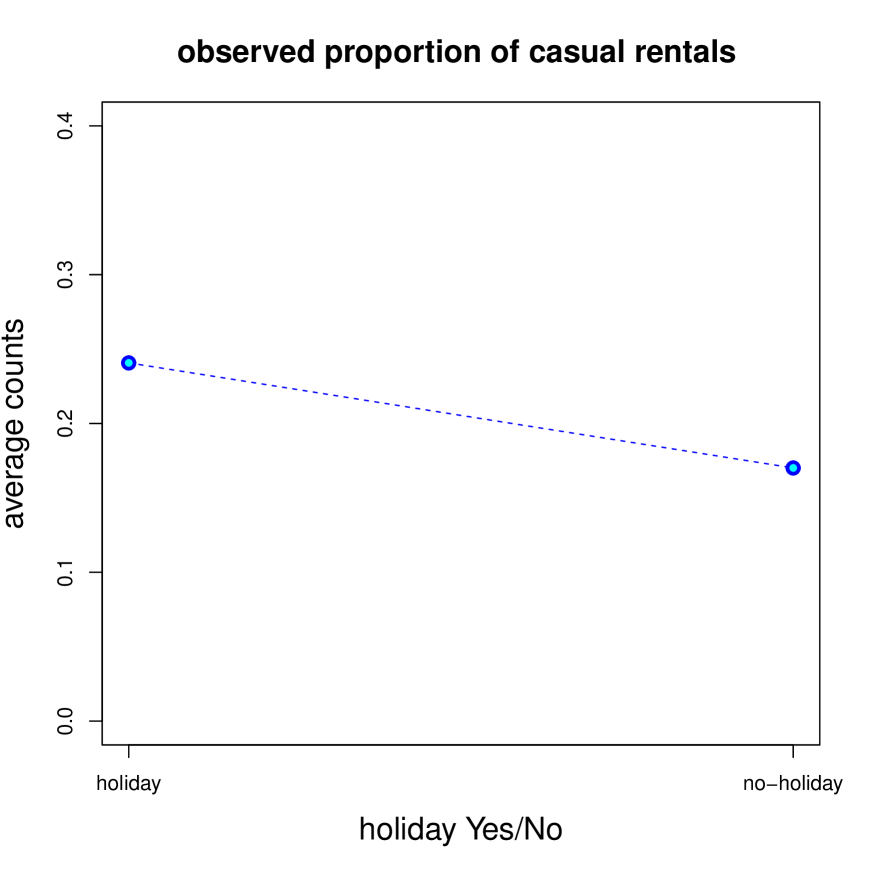
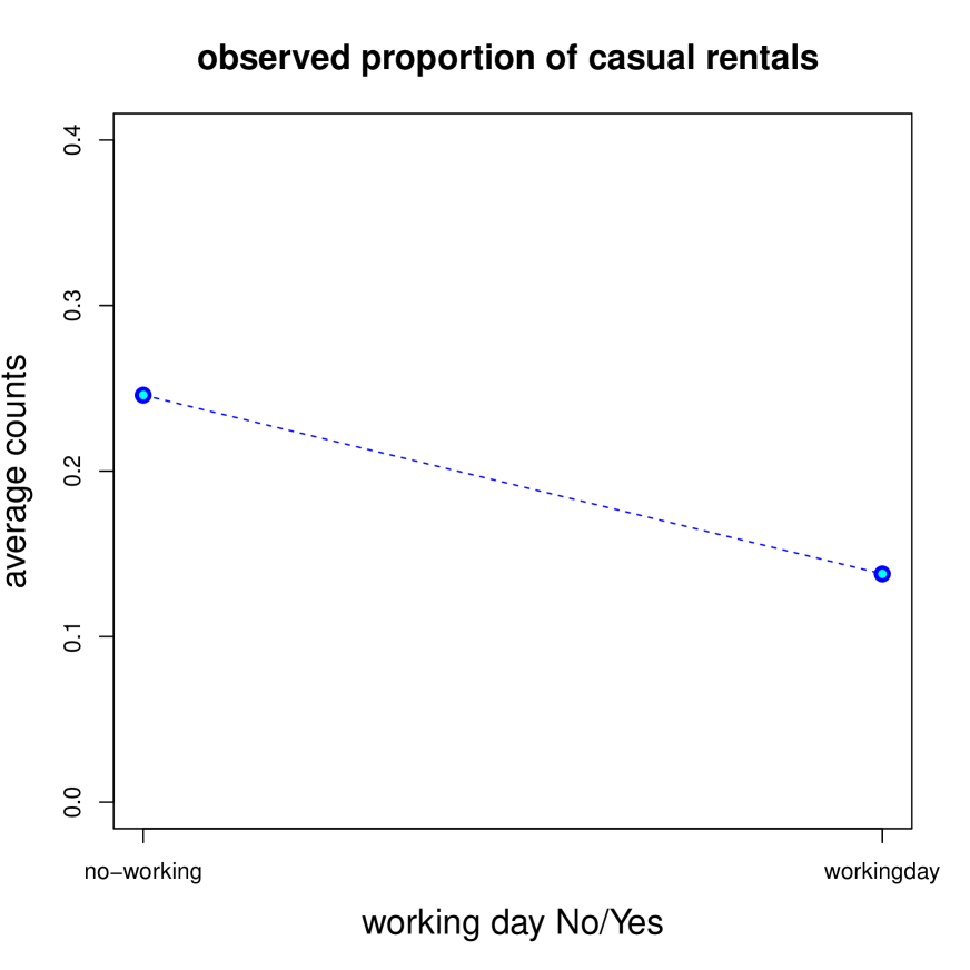
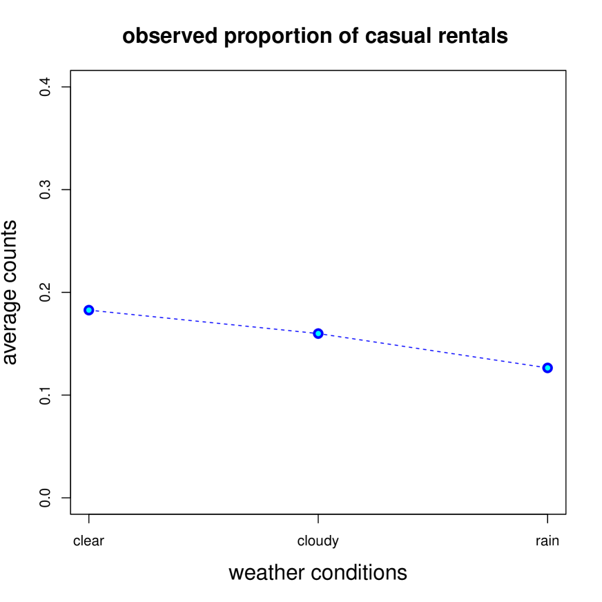
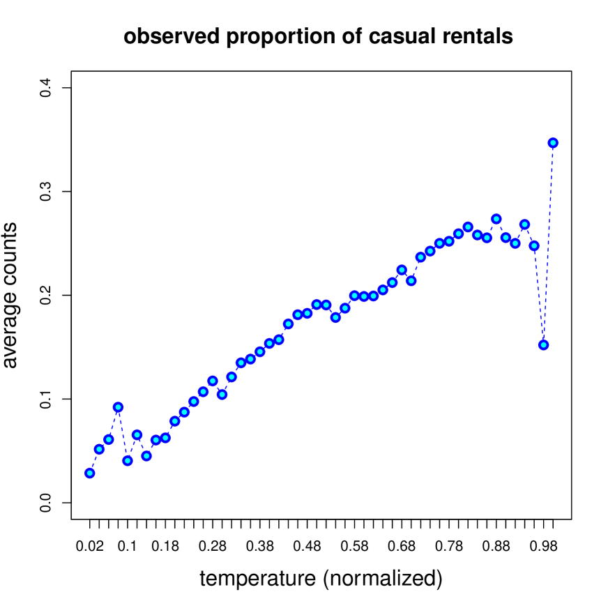
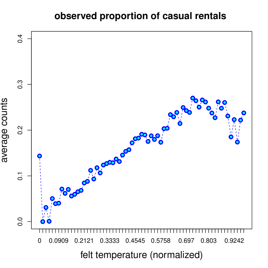
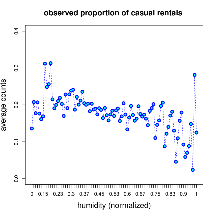
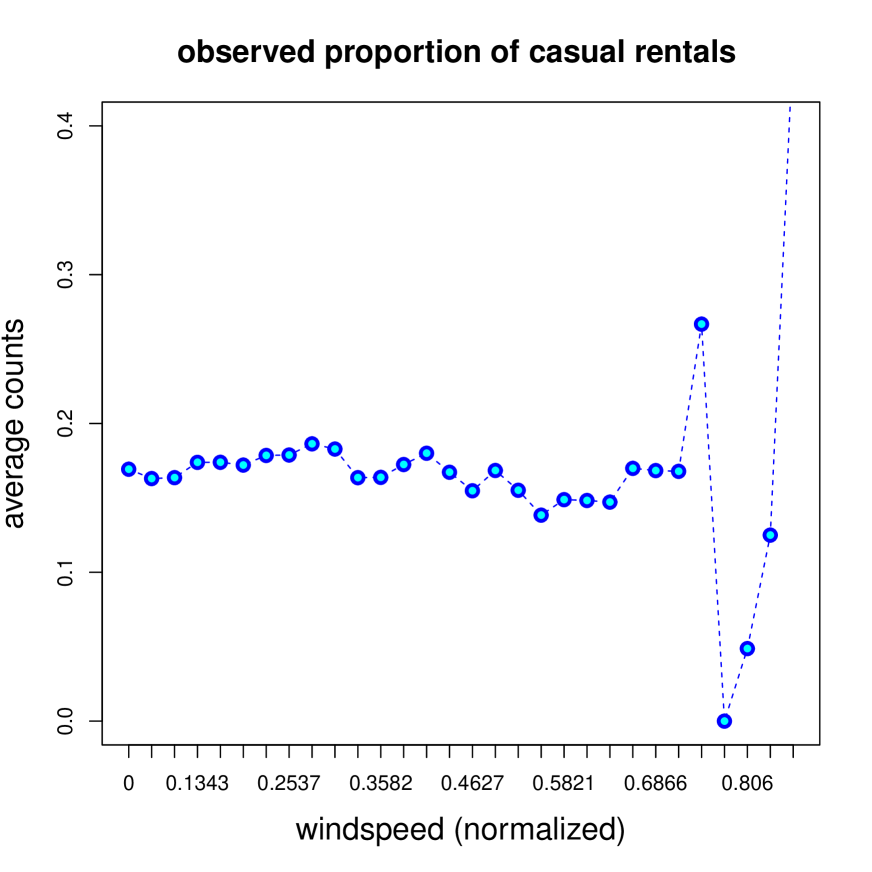
Figure 12: Average response $Y$ for each label of all features date (in weekly units), year, month, hour, weekday, holiday, workingday, weather, temp, temp_feel, humidity and windspeed.

In Figure 12 we provide the marginal observed responses for each label of all features. The top-left shows the average response for each calendar week from 2011/01/01 until 2012/12/31. This depicts a strong seasonal pattern of the casual rentals proportion. Moreover, daytime, weekdays, working days/holidays and weather conditions such as temperature is important information for predicting the proportion of casual rentals. Only wind speed does not seem to be very relevant. From the top-middle we also observe that the proportion of casual rentals slightly decreases over time which can be explained by increasing regular rental subscriptions from 2011 to 2012.

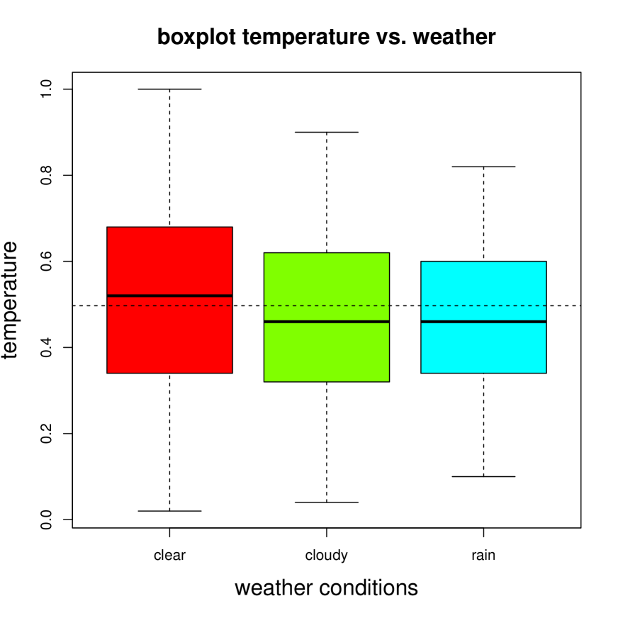
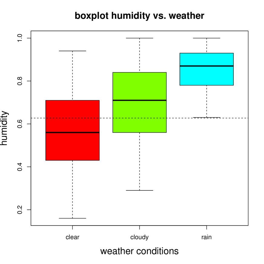
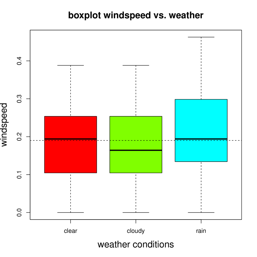
Figure 13: Dependence between feature components: (top) temperature, humidity and wind speed against calendar month, (middle) temperature, humidity and wind speed against daytime, (bottom) temperature, humidity and wind speed against weather conditions.

For many of the feature components it is clear that they are highly correlated. In Figure 13 we plot temperature, humidity and wind speed against calendar month (top row), daytime (middle row) and weather conditions (bottom row). These plots clearly show this dependence. Moreover, humidity is negatively correlated with wind speed and positively correlated with temperature (at least up to moderate temperatures).

References

- [TensorFlow 2015] Abadi, M., et al. (2015) TensorFlow: large-scale machine learning on heterogeneous systems. https://www.tensorflow.org/
- [Acerci 2002] Acerbi, C. (2002). Spectral measures of risk: a coherent representation of subjective risk aversion. Journal of Banking and Finance 7, 1505-1518.
- [Ancona et al. 2019] Ancona, M., Ceolini, E., Öztireli, C., Gross, M. (2019). Gradient-based attribution methods. In: Explainable AI: Interpreting, Explaining and Visualizing Deep Learning. Samek, W., Montavon, G., Vedaldi, A., Hansen, L.K., Müller K.-R. (Eds.). Springer, Lecture Notes in Artificial Intelligence 11700, 168-191.
- [Apley and Zhu 2020] Apley, D.W., Zhu, J. (2020). Visualizing the effects of predictor variables in black box supervised learning models. Journal of the Royal Statistical Society: Series B 82/4, 1059-1086
- [Bengio et al. 2003] Bengio Y., Ducharme R., Vincent P., Jauvin C. (2003). A neural probabilistic language model. Journal of Machine Learning Research 3/Feb, 1137-1155.
- [Binder et al. 2016] Binder, A., Bach, S., Montavon, G., Müller K.-R., Samek, W. (2016). Layer-wise relevance propagation for deep neural network architectures. In: Information Science and Applications (ICISA). Kim K., Joukov N. (Eds.). Springer, Lecture Notes in Electrical Engineering 376.
- [Breiman 2001] Breiman, L. (2001). Random forests. Machine Learning 45/1, 5-32.
- [Keras 2015] Chollet, F., et al. (2015). Keras. https://github.com/fchollet/keras
- [Dietterich 2000a] Dietterich, T.G. (2000). An experimental comparison of three methods for constructing ensembles of decision trees: bagging, boosting, and randomization. Machine Learning 40/2, 139-157.
- [Dietterich 2000b] Dietterich, T.G. (2000). Ensemble methods in machine learning. In: Multiple Classifier Systems, J. Kittel, F. Roli (eds.). Lecture Notes in Computer Science, 1857, Springer, 1-15.
- [Efron 2020] Efron, B. (2020). Prediction, estimation and attribution. International Statistical Review 88/S1, S28-S59.
- [Fanaee-T and Gama 2014] Fanaee-T, H. , Gama, J. (2014). Event labeling combining ensemble detectors and background knowledge. Progress in Artificial Intelligence 2, 113-127.
- [Friedman 2001] Friedman, J.H. (2001). Greedy function approximation: a gradient boosting machine. Annals of Statistics 29/5, 1189-1232.