Many-body localization in tilted and harmonic potentials
Abstract
We discuss nonergodic dynamics of interacting spinless fermions in a tilted optical lattice as modeled by XXZ spin chain in magnetic (or electric) field changing linearly across the chain. The time dynamics is studied using exact propagation for small chains and matrix product states techniques for larger system sizes. We consider both the initial Néel separable state as well as the quantum quench scenario in which the initial state may be significantly entangled. We show that the entanglement dynamics is significantly different in both cases. In the former a rapid initial growth is followed by a saturation for sufficiently large tilt, . In the latter case the dynamics seems to be dominated by pair tunneling and the effective tunneling rate scales as . In the presence of an additional harmonic potential the imbalance is found to be entirely determined by a local effective tilt, , the entanglement entropy growth is modulated with frequency that follows scaling first but at long time the dynamics is determined rather by the curvature of the harmonic potential. Only for large tilts or sufficiently large curvatures, corresponding to the deeply localized regime, we find the logarithmic entanglement growth for Néel initial state. The same curvature determines long-time imbalance for large which reveals strong revival phenomena associated with the manifold of equally spaced states, degenerate in the absence of the harmonic potential.
I Introduction
Many-body localization (MBL) became a well established property of interacting many-body systems in sufficiently strong disordered potentials. Seminal works [1, 2] started a chain of research resulting in hundred of research papers (to see some of the early works, consult [3, 4]) partially summarized in recent reviews [5, 6, 7, 8]. MBL is considered as a robust counterexample to thermalization, as localization is supposed to lead to the memory effect of the initial state in the closed system in contrary to the eigenstate thermalization hypothesis [9, 10] predictions. Yet, a recent work [11] put the very existence of MBL in the thermodynamic limit in question stimulating an intensive debate [12, 13, 14, 15, 16, 17] mainly based on results coming from exact diagonalization studies, necessarily limited to small system sizes. Matrix product states (MPS) techniques allow one to consider large system sizes [18, 19, 20, 21, 22, 23]. Then the transition to MBL is studied addressing long time dependence of certain correlation function (the so called imbalance, see below) [24, 25, 26, 27, 28, 29] mimicking experimental scenarios [30, 31]. Still these claims are not definitely conclusive due to finite systems sizes and, importantly, rather short evolution times taken into consideration, limited by the numerical methods, such as the time-dependent variational principle (TDVP).
Recently, it was also observed that a constant strong tilt of the optical lattice may lead to nonergodic behavior in the presence of a small disorder [32] or even in the absence of it [33]. The phenomenon, usually referred to as the Stark many-body localization (SMBL), is an extension of Wannier-Stark localization for non-interacting particles [34]. Interestingly, for a pure constant tilt the dynamics is a bit peculiar, e.g., the entanglement entropy shows a strong initial growth for an initial separable state [33], a phenomenon associated to the fact that such an initial state is degenerate with the number of other separable states of the same global dipole moment (see below). On the other hand, with addition of a small disorder, or an additional weak harmonic potential SMBL shows features very similar to a standard MBL such as the logarithmic entanglement entropy growth [33], Poissonian level spacing statistics [32, 33], a power-law decay of a double electron-electron resonance (DEER) (introduced by [35]) signal or a logarithmic growth of quantum mutual information [36]. The role of the harmonic confinement was further analyzed in [37] where it was shown, in particular, that a smooth site-dependent chemical potential leads to an effective local static field related to the derivative of this potential with respect to the spatial dimension. For strong harmonic term that may lead to phase separation between localized and delocalized phases [37, 38]. To complete the picture, let us also note that SMBL is also addressed recently for open systems [39].
While spinless fermions have been considered theoretically (bosons have been discussed in [36, 40]), the experiments with cold atoms considered spinful fermions both in two-dimensional (2D) setup [41] and in a single dimension (1D) [42]. SMBL has been also studied on superconducting quantum processor [43] emulating a spin-1/2 chain in a triangular ladder as well as, very recently, on an trapped ion quantum simulator [44], where the coexistence of localized and delocalized phases in a strong harmonic potential [37] has been verified.
The unusual time dynamics of pure tilted case (by a pure case we shall consider the situation with the ideal linear lattice tilt with no additional harmonic or other local potential) may be better understood using the concept of the emergent dipole moment conservation [41]. Due to superextensive character of the tilted potential term, the energy accumulated in the potential energy related to the tilt may not, sometimes change entirely into the kinetic energy leading to the memory of the initial state. This point has been further elaborated in [45] using the concept of shattered Hilbert space. State possessing initially a large (in absolute value) dipole moment may not undergo thermalization. This has been visualized in [46] for domain wall states also for a relatively small tilt when the majority of separable initial states thermalizes fast. Their existence may be also traced back to a peculiar feature of the Heisenberg model used – the domain containing spins with the same orientation (up or down oriented spins) is practically frozen in the dynamics for the time dependent on the length of the domain. So local thermalization occurs at domain walls only [46, 38].
The aim of this contribution is to provide a detailed insight into the dynamics of both pure tilt case as well as a harmonically perturbed model. We consider small system sizes with large integration times together with larger systems treated using time dependent variational principle (TDVP) algorithm [21, 47, 23]. We analyze in detail different contributions to the entanglement entropy and their time dynamics. Importantly, apart from the dynamics of initial separable Néel state, we consider also the quantum quench scenario [48, 49] for a pure tilt case used previously for disordered systems. That allows us to provide insight into the long time entanglement growth. In the presence of an additional harmonic trap we verify the transition to a more standard, MBL-like behavior [33, 36] although we observe a logarithmic growth of the entanglement entropy in the deeply localized regime only. Most importantly, we stress the importance of the concept of local tilt, i.e., the spatial derivative of the continuously varying chemical potential. Specifically, we show that the dynamics can be described entirely by the local tilt in cases of both pure tilt and with the addition of harmonic potential when viewed through the eye of time-evolved local imbalance. This is due to the fact that a particular site is only affected by few neighboring sites during the evolution because of strong localization rendering the dynamics very much local in space. On the other hand, as mentioned before, addition of harmonic potential greatly changes the dynamics of entanglement entropy. However, we show that the concept of local tilt still remains valid for entanglement entropy within the scenarios of harmonically perturbed systems. Furthermore, for sufficiently large tilt, we provide an evidence of quantum revivals present in the (easily accessible to experiments) imbalance as well as reflected in the entropy dynamics.
II The model
We consider the paradigmatic model in MBL studies, namely the XXZ spin chain with the Hamiltonian
| (1) |
with ’s being spin-1/2 operators and being the onsite potential. In typical MBL studies [50, 7, 51, 13], is a diagonal disorder (a magnetic field along -axis) drawn from random uniform distribution. We consider instead where is the magnitude of the linear tilt and is (twice) the curvature of the additional harmonic potential. Note that while for case it may be convenient to center the harmonic potential with respect to the chain (so it forms a confining potential [37, 40]). Here we follow a different setting [33, 36]. We also set as the energy unit. For the model reduces to the Heisenberg chain. Using Jordan-Wigner transformation the model reduces to the case of spinless fermions tunneling with the rate and with the nearest neighbor interaction . Unless explicitly stated otherwise, we shall mostly concentrate on the dynamics of the Heisenberg chain.
We mostly consider time dynamics starting from the initial Néel state with every odd spin pointing up, and every even down (remaining in the conserved total sector). While Ref. [33] averaged the dynamics over different possible states, we choose the Néel state that corresponds, after Jordan-Wigner transformation, to an equivalent density wave state with occupied odd sites and empty even sites in the spinless fermion representation in analogy to the experimental situation [31].
We characterize the state of the system by considering the spin correlation function which, for the Néel state, is equivalent to the imbalance of occupations between odd and even sites in the fermionic picture:
| (2) |
where , denote the total occupation of even and odd sites. We use also the entanglement entropy by splitting the system in two parts and . Defining the reduced density matrix where is the time evolved state of the system, the entanglement entropy reads where are the eigenvalues of . Interestingly, owing to the global symmetry of total conservation, the entanglement entropy may be split into the sum of classical number entropy and the quantum configuration entropy : [52, 53, 54, 55, 56] with
| (3) |
where we denoted by the probability of populating the -particle sector in subsystem A and by the corresponding block of the density matrix for the subsystem A, such that . The number entropy describes a real transfer of particles between the subsystems considered and the configuration entropy, , quantifies the possible arrangements of particles on each side of the system.
III Pure tilt case
Let us consider first the dynamics in the pure tilted case with . We shall consider both small systems amenable to exact diagonalization as in [33, 32, 36] as well as more realistic systems sizes using TDVP. To check convergence we have also compared TDVP and TEBD results as in [29] – see Appendix A. For a purely deterministic potential no averaging over disorder realizations, as in case of random potentials, is possible. Typically we shall consider small systems of size and compare those with cases analyzed with TDVP.
III.1 Initial Néel state
As announced in the previous section we consider the time dynamics of the initial Néel state.
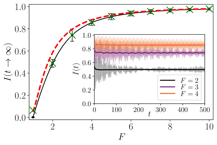
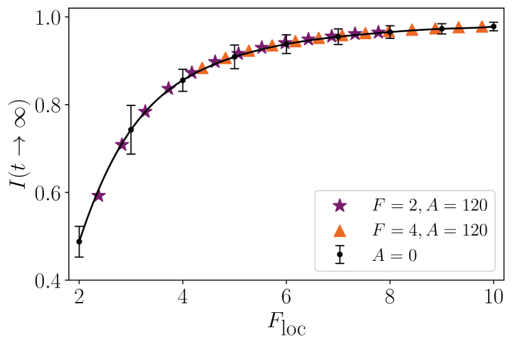
Consider first the “experimental” evidence for SMBL, i.e., the existence of a non-zero imbalance at large times indicating the preservation of the memory about the initial state during time evolution. The imbalance at saturation occurring at large times is presented in Fig. 1. The data are averaged over to wash out the rapid oscillations of the time-dependent signal (as shown in the inset). Data are obtained with TDVP with . The errors indicated in the figure are due to these fast oscillations and are standard statistical errors. The data indicate that the crossover to delocalized phase appears at , in agreement with the data for small system sizes obtained from level statistics [33, 32]. One should, however, keep in mind that the accuracy of long time TDVP simulations close to the transition deteriorates, so that the critical value should be taken with caution as the result becomes a compromise between the duration of the time propagation and the limitation on the assumed auxiliary space dimension, . Note, however, a very good agreement for between long time imbalance value for obtained via TDVP and obtained via exact diagonalization-based propagation. In both cases 4 sites at each edge of the system were excluded from calculation of the imbalance to minimize open boundary effects. Also note, to some extent disappointingly, that the final imbalance is quite close to the analytic prediction for the noninteracting case, i.e., pure Wannier-Stark localization [42]
| (4) |
where represents the zeroth-order Bessel function, especially for large that suggests the decreasing importance of interactions for large .
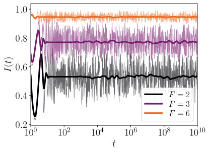
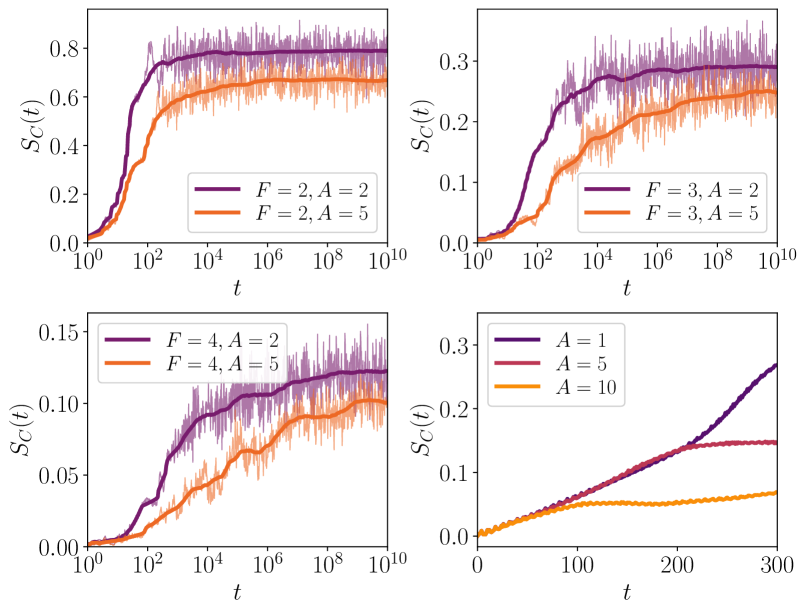
Left panel of Fig. 2 shows a typical imbalance as a function of time for a few values of the static tilt, for small system size but for much longer times. Observe quite large fast changes of which reflect short range jumps of fermions (spin flips in the spin language) between nearby sites. Those are the remnants of Bloch oscillations for noninteracting system [42] in our interacting case. To get the information beyond these rapid changes we apply a frequency filter that effectively averages our fast oscillations. The filter smoothly cuts out large frequencies in the Fourier transform of the signal – for a detailed description of the filter see the Appendix B. The effective, time-averaged signal is also shown in Fig. 1.
The right panel of Fig. 2 shows the entanglement entropy growth with time. Here an initial rather rapid growth is also followed by a saturation for sufficiently large tilts as taken for the plots. The values of the tilt correspond to the “localized” regime according to spectral properties – the localization transition is estimated at in the large system-size limit [32] (note that different units are used in that work, the value given there is twice bigger). Let us recall that one of the hallmarks of MBL is the logarithmic growth of the entanglement entropy for initially separable states [57, 58]. The growth of the entanglement entropy for SMBL is apparently quite different. Moreover, the fast saturation of the entanglement entropy with time is in apparent contradiction with the result shown in [33] where the entanglement entropy, after a fast initial rise, grows slowly for long times too. This is due, in our opinion, to a different initial state assumed. We take an ideal Néel state while in [33] an average over initial states with the same density per site but having no initial occupation on sites between which the cut into A and B subsystems is made. Thus among states included in [33] are, e.g., states with domain walls – extended regions of identically oriented spins that may result in excessively slow dynamics due to frozen spins [46, 38].
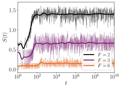
While Fig. 2 presents the results for a relatively large tilt, deep in the localized regime, Fig. 3 presents the time evolution of the entanglement entropy for tilt values close to the transition. Here we split the entropy into the classical number entropy (left panel) and the configuration entropy (right panel) as described by (3). Observe that for both entropy components the fast growth and the saturation part are separated by an intermediate stage of logarithmic entropy growth. As pointed out in [33, 36] the fast initial entropy growth is related to degenerate manifold of states leading to the entanglement build-up. For moderate tilt the localization takes some time to settle in leading to an intermediate logarithmic growth resembling MBL. This region of values, say , corresponds to the transition region between delocalized and SMBL phases in the spectral analysis [32].
Let us note also that the saturation of the number entropy at low values at later times makes the localization observed distinctly different from disorder induced MBL where a very slow is observed [59, 60]. Here for MBL also an eventual saturation is predicted [61] due to single particle exchange across the analyzed bond but the corresponding saturation value is much higher than observed by us in SMBL (compare Fig. 3).
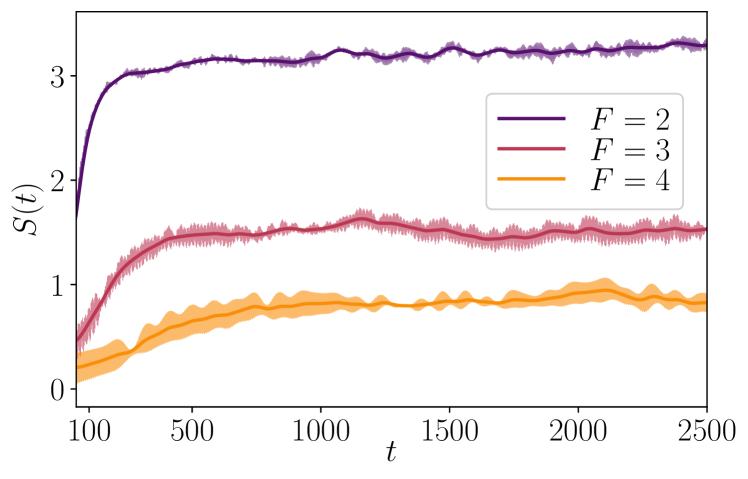
These observations are further exemplified for larger system sizes using TDVP simulations. The entanglement entropy growth on the middle bond is shown in Fig 4. Strong high frequency oscillations can be averaged out leading to solid lines. Two time-regimes may be again clearly identified. The first is the region of a linear growth of entropy with time which extends to larger times for bigger . The second regime, for sufficiently long times and larger corresponds to an apparent saturation of the entanglement entropy. Data for and larger clearly saturate while for lower we observe a fast linear growth for short times followed by a slow linear drift without saturation. We cannot determine whether this drift is linear or logarithmic in time due to a limited time span and small changes of the entropy.
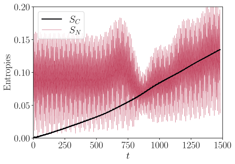
For even stronger tilts the entropy reveals relatively larger fast oscillations as shown in Fig. 5. It is the classical number entropy which is responsible for oscillations in the localized regime. It is thus related to a transfer of a single particle across the analyzed bond and is similar in its origin to Bloch oscillations. On the other hand, the quantum part of the entanglement entropy, the configuration entropy, shows smooth practically linear increase in time with a slight bending upwards. Note that for large value shown, this growth is quite small in the absolute sense.
III.2 Quantum quench
Let us consider a different scenario of initial state preparation. Instead of initial separable state we consider a quantum quench approach [48]. We prepare the ground state of the system for some initial parameters and then rapidly change them to the final values at which the time-evolution takes place. By a judicious choice of quenched parameters one may probe different energies of the final Hamiltonian. The method has been shown to be effective in a variety of models [48, 62, 49] allowing to pin down the possible existence of mobility edges.
In the present situation we prepare the system, at some given interaction strength and in the absence of any tilt in the ground state of Hamiltonian (1). Then we rapidly turn on the tilt and observe the time dynamics. The ground state of XXZ depends on : for , the interaction energy dominates and ground state is of a gapped antiferromagnetic order while for the ground state is in critical XY phase. The ground state itself has non-vanishing entanglement because of non-zero interaction, and we study the change of configurational entropy after the quench. The growth of brings us the information of how quantum entanglement further builds up in the system.
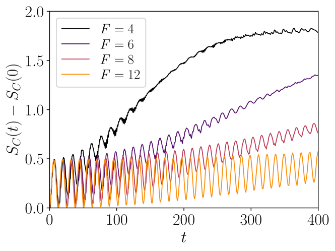
Consider the tilt quench (from zero to different final values) for in which case the initial ground state is antiferromagnetic. While this state is not separable it resembles the Néel separable state. The corresponding entanglement entropy growth is thus similar to that observed previously – compare the right panel of Fig. 6 where we show the configuration entropy growth from its initial nonzero value. The configurational entropy builds slowly initially, and then subsequent rather fast growth ends with a rapid saturation at a fixed dependent value. The situation is markedly different for the critical initial state (). Here the initial stage for different values is similar revealing fast oscillations. As shown in the Appendix C the frequency of these oscillations depends linearly on indicating that the rearrangement of particles is governed by interactions.
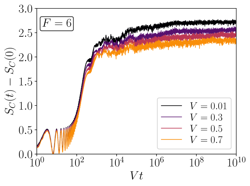
Beyond the initial oscillation stage, the configuration entropy (we shall consider in detail quench case as entirely different from the Néel initial state situation) rapidly grows in dependent manner. However, as shown in the right panel of Fig. 7 this rapid growth falls onto a single curve by rescaling the time by factor. By separately analyzing different cases (see Appendix C for the evidence) one observes that the correct scaling of time in this region is . This numerically identified scaling is explained extending the mechanism of particle redistributions discussed in detail in [36]. Consider two particles in a strong field . For strong tilt the associated energy dominates other energy contributions, the dipole moment of two particles, or its center of mass is quasi-conserved. Now take an initial configuration , which appears primarily for smaller interactions , being replaced by density wave configurations for larger . The thermalization of states involves spreading out of these two adjacent particles, but under such a strong field , they can not break the dipole conservation. Thus one is left with the effective tunneling of particle pairs, , that transfers . By second order perturbation theory we obtain
| (5) |
providing the explanation for the scaling factor. Higher order contributions, again preserving the dipole moment will lead to successive orders , . Since a higher order term has much smaller value, it dominates the dynamics after all dynamics before it is completed.
IV Cooperation of the tilted and harmonic potentials
Consider now the model in which the constant tilt is supplemented by the harmonic potential. As studied in some detail in [33, 36] the localization in this case is quite similar to MBL. In particular a logarithmic growth of the entanglement entropy is being observed as the additional harmonic term in the potential lifts the partial degeneracy of the spectrum in a pure tilted case. In a different study [37] we have considered the dynamics in a harmonic potential alone (with no tilt) finding that localized and delocalized regions may coexist in different parts of the chain, the phenomenon confirmed experimentally recently [44]. Importantly, it turned out that the border between localized and delocalized regions is well predicted involving the notion of the effective local field which for the harmonic potential of the form equals . The transition occurred whenever , separating the regions of smaller and larger local field. This behavior is easily understood as many-body localization length in real space is very small, and also for Stark localization it extends over few sites only. With the assumed chemical potential in the form the local field becomes (note that the curvature of the potential is in our convention equal to ).
For a pure tilt we were able to relate the tilt with the final imbalance value – see Fig. 1. Now, in the presence of the additional harmonic potential the local field changes along the chain and no such a simple connection to the final global imbalance can be made. However, one may define a local imbalance comparing occupations of just two sites and . For the initial Néel state, at one site the spin is up, at the other down (corresponding to occupied and empty sites in the fermionic language) initially, and the change of spin orientation with time may be analyzed. Let us define a local imbalance:
| (6) |
centered, to be precise, in the middle of the bond linking site with . With this position we can associate, for a given and a local field . For , and the local imbalance is the same for all (again we drop sites very close to the edges of the system) and equals the global imbalance plotted already in Fig. 1.
The comparison of local imbalance for different values is shown in Fig. 8 as a function of . Observe that data for different lie on an universal curve. Thus the local imbalance is solely determined by . This result is even more spectacular keeping in mind the drastically different growth of entanglement entropy for pure tilt and in the presence of an additional harmonic component.
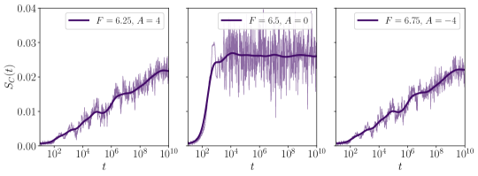
However, the local field approach, while so successful for imbalance must partially fail for the entanglement entropy growth which substantially differs in the presence or absence of the harmonic component as discussed previously [33, 36]. This is further exemplified in Fig. 9 for the Néel initial state where we consider configuration (quantum) part of the entanglement entropy, the most relevant one in the localized regime (recall that the number entropy shows large oscillations - Fig. 5). While in the absence of the harmonic potential (central panel) the fast growth is followed by a saturation, the presence of the harmonic component in the potential makes the growth almost logarithmic in time, with superimposed small oscillations. Note that, surprizingly both left and right panels look very similar despite the fact that the harmonic component has either positive or negative curvature. It seems, that once we disregard the pure tilt case as special, the local field (same for both panels) provide some information on the configuration entropy growth.
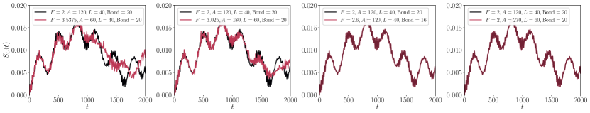
This importance of the local field for configuration entropy dynamics is further evidenced in Fig. 10. The configuration entropy time dependence for the bond (i.e., the bond between sites and ), , , and (corresponding to the curvature in the lattice spacing units) is compared with similar cases for different tilt and curvature components, as well as different system size but sharing the same value of the local field on the analyzed bond. Interestingly, for quite a long time it seems that it is this local field value which determines the entropy dynamics as curves coincide roughly up to (which seems to be at the edge of experimental feasibility [42]). Only for later times the difference appear. They are canceled provided both and the curvature of the harmonic component are the same. This may be understood in a simple perturbative picture in which the harmonic potential contribution to the dynamics starts to play some role after a sufficient time. It is to be noted that in the noninteracting case, i.e., , the configurational entropy remains practically zero for the above choices of parameters.
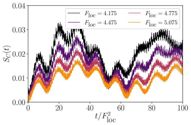
The scaling of initial oscillations of the configuration entropy may be identified by looking at different values. Those can be obtained from a single run with nonzero curvature, we consider the case represented by black curve in Fig. 10. As it turns out the correct scaling of time occurs for factor – see Fig. 11. Let us recall the explanation of the scaling scenario in Stark regime in terms of simultaneous tunneling of two particles as “conserving the global dipole moment”. Here apparently we have a similar scenario but due to the presence of the harmonic potential, takes the role of .
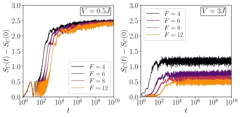
As shown in Fig. 9 in the presence of a harmonic confinement and a large tilt, the long time entanglement entropy growth seems to follow mean growth with additional oscillations which we just analyzed. Similar logarithmic growth has been stressed in earlier studies [33, 36]. This is not always the case as exemplified in Fig. 12. For a Néel initial state the logarithmic growth of the configuration (and thus total) entanglement entropy starts to appear for sufficiently large and . For weaker tilt, as in the top row, small system studies (that enable long time dynamics studies) indicate that the initial, rather fast entropy growth is followed by a saturation as for pure tilt case. Apparently, for lifting of degeneracies induced by a harmonic field is not sufficient. During the short initial time the system does not resolve individual levels and the entropy grows in a way resembling a pure linear tilt. Then the saturation of the entanglement entropy growth due to -field localization prevents further growth. With increasing the transition to a more “standard” logarithmic growth is observed for sufficiently large and (bottom left panel of Fig. 12).
Our findings in terms of entanglement entropy growth are apparently at variance with results reported in [33, 36] that stress the similarity of SMBL in additional harmonic potential and the standard MBL, in particular showing the logarithmic entropy growth. This discrepancy may be due to different initial states. We considered experimentally relevant Néel initial state while, e.g., [33] averages over different initial states empty close to the bond on which entropy is calculated. Averaging over different initial states with significantly different dynamics may result in the average entropy growth different from that observed for the Néel state. This aspect requires a separate detailed study.
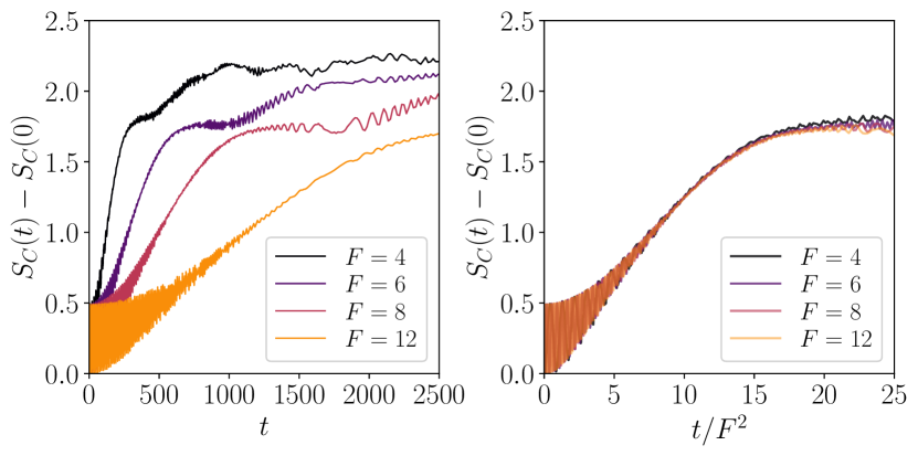
The bottom-right panel illustrates the time dynamics for short times (but for larger system) exemplifying the initial linear growth associated to degeneracies of the spectra for pure linear tilt [33, 36]. With increasing curvature the linear growth is followed for a shorter time, while the system realizes that the degeneracy is lifted, the growth becomes slowed and undergoes oscillations discussed above.
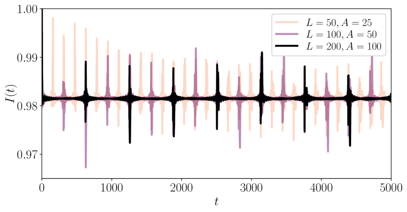
Lastly, let us consider in detail the time dependence of the imbalance for different system sizes and different curvatures of the harmonic potential for even larger tilts. For the imbalance saturates very fast at the high value about 0.98 showing, however, regular revivals. We have verified that the period of the revivals does not depend of , the resulting curves are similar for or at different saturation level. For each system size the value is chosen in such a way that a local field at the end of the chain is increased from to . To a good precision the period of revivals equals as if corresponding to equally spaced levels with spacing . Indeed by a direct evaluation (calculations were performed at small sizes) one may check that the (quasi-)degenerate (for ) manifold of states having the same global dipole moment splits in the presence of the additional harmonic potential of curvature into the set of almost equally spaced levels with the spacing . However, only every second state in this manifold has a non-zero overlap with the initial Néel state contributing to the dynamics – thus indeed the relevant spacing is equal to . Another important point to note is that since the emerging dipole conservation becomes exact only in the large limit, such revivals with period become more pronounced with increasing .
V Conclusions
We performed a detailed analysis of localization in disorder-free potentials considering both the pure static field and the system with an additional weak harmonic potential. We have studied both small system sizes where exact diagonalization and Chebyshev propagation enables accurate results for very long times, as well as large systems have been studied with the help of matrix product states algorithms. By a detailed analysis of the entanglement entropy we have verified that the character of localization in a pure static field is different from standard disorder induced MBL, in particular a fast initial growth of the entanglement entropy in a static field followed by a full saturation is different from the logarithmic growth known from MBL. Similarly while the number entropy in the standard MBL seems to grow as [59, 60] at long times - we observe strong fast Bloch-like oscillations, but filtering them out we observe no trace of the slow -like growth. The rapid initial growth of the entanglement entropy can be associated with a rapid coherent coupling within the degenerate manifold for the pure tilt [33, 36]. The large system size data provide a further confirmation for these claims.
Apart from the time dynamics of the initial Néel state we considered also a quantum quench scenario. There we have identified the mechanism of the entanglement entropy growth in the localized regime as an effective second order tunneling of two particles conserving the emergent global dipole moment.
In the presence of an additional harmonic potential the character of the dynamics changes. While the resemblance to the standard MBL was noted in [33, 36] in, e.g., the logarithmic growth of the entanglement entropy in time, our simulations for the Néel initial state show this to be the case only for sufficiently large tilt and curvature of the harmonic potential. This observation is limited to small systems only as it requires long evolution times. For shorter, experimentally reachable times we analyze the large period oscillations of the configuration entropy and observe there the characteristic time scales related to the local tilt values (at the bond where entanglement is analyzed). The detailed analysis of the imbalance from the initial Néel state as well as the entanglement entropy dynamics indicates that while “local” field approximation introduced by us in [37] may provide very good estimate for the system behavior, it fails for long times in providing a consistent interpretation of the entanglement entropy time dynamics. There an additional influence of the potential curvature must be taken into account to explain the simulation results. Studying large systems we have shown that breaking of the approximate global dipole conservation may also result, in the strongly localized regime, in the appearance of the characteristic revivals in the long time imbalance.
Finally we would like to stress that the word of caution is necessary. While for small systems we may access large times by exact propagation we cannot do so for larger systems where we use TDVP. So the physics of large systems and long times in tilted potentials may hide additional surprizes. In particular, in the limit of large tilt we may expect to observe unusual thermalization due to fractonic dynamics [63, 64, 65, 66, 36, 45] which is, however, beyond the scope of this work.
Acknowledgements.
This work benefited from the invaluable input of Dominique Delande who contributed dominantly to the TEBD parallelized code used in this work. Equally important were discussions with Piotr Sierant on various aspects of the physics of tilted models. We acknowledge both contributions. J.Z. is grateful to Pablo Sala for suggesting the comparison of imbalance to the noninteracting case. Discussion with Frank Pollmann was also very enlightening. The numerical computations have been possible thanks to High-Performance Computing Platform of Peking University as well as PL-Grid Infrastructure. The TDVP simulations have been performed using ITensor library (https://itensor.org). This research has been supported by National Science Centre (Poland) under projects 2017/25/Z/ST2/03029 (T.C.) and 2019/35/B/ST2/00034 (J.Z.)Appendix A Remarks on matrix product states based time dynamics for large systems
The study of larger systems is possible entirely within the necessarily approximate time-dynamics schemes such as time-evolving-block-decimation (TEBD) [18], time-dependent density matrix renormalization group tDMRG [19], or more recent numerical schemes based on time dependent variational principle (TDVP) [21, 47, 23]. The early studies involved TEBD [18, 20, 67, 68] that allowed for relatively efficient simulation of interacting systems also in the context of MBL [69, 24, 25, 26]. Recently TDVP was used by the Karlsruhe group to estimate the onset of MBL in large systems [70, 27] – for a discussion see [71]. The latter work critically inspected applicability of TEBD and TDVP for accurate description of time-dynamics in systems of realistic size. In this work, we mostly use a hybrid variation of the TDVP scheme [23, 72, 29, 71], where we first use two-site version of TDVP. At this stage the (auxiliary) bond dimension grows up to a prescribed value. Reaching , we switch to the one-site version (avoiding errors due to a truncation of singular values in the two-site version [23, 72]). Typically for large , in the localized regime, we often do not reach so the simulations are fully converged (up to numerical errors). For TEBD we use an efficiently parallelized home made package that utilizes the recent breakthrough for Lie-Trotter-Suzuki decomposition [73]. . Disappointingly, the execution times needed for propagation using TDVP of realistic system sizes in a static tilt case were found empirically to be quite long compared to disordered scenarios. This may be related to the fact that in presence of static fields the energy levels of the Hamiltonian are spread covering a broad range of energies and local Lanczos exponentiations in the TDVP scheme require large Krylov space to converge. On the other hand the simulations, in the absence of disorder, require just a single run, with no disorder averaging. That, with a necessary patience, allows us to study system sizes and times unprecedented until now.
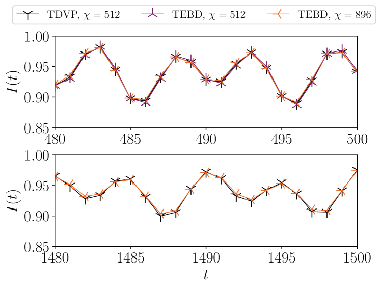
To test the accuracy of our studies we compare the simulations performed with TDVP, where due to the sweeping procedure, an efficient parallelization of the code seems difficult, with TEBD where such a parallelized code with higher order Suzuki-Trotter scheme is possible. Fig. 14 shows that the imbalance evolution in time for a state in the localized regime is essentially the same using TDVP and TEBD propagation schemes. Since, as shown in [71] TEBD overestimates the imbalance while TDVP underestimates it, the agreement of both schemes assures that the results obtained are fully converged. Note that even deep in the localized regime we have to use slightly larger auxiliary space dimension for TEBD, as described in the caption of Fig. 14 - the possible growth in the execution time is compensated by efficient parallelization possible for TEBD. Note also that we do not observe any sign of the accumulated Trotter errors which haunts TEBD implementation [20] – presumably because of high order decomposition used [73].
Appendix B The frequency filter
To minimize the effects of high frequency oscillations in the time signal of a particular observable, say , we first perform the fast Fourier transform (FFT) in the time domain as . Then we perform a Gaussian convolution to the Fourier transformed data as for reducing the contributions coming from higher frequencies. Finally, an inverse fast Fourier transform (iFFT) is performed to get the frequency filtered data in the time domain as . In our calculations, we have used NumPy’s standard FFT and iFFT functions (https://numpy.org/doc/stable/reference/routines.fft.html), and have chosen the standard deviation in the Gaussian convolution between depending on the scenarios.
Appendix C Details on quantum quench properties
We take a closer look at weak interaction case by examining different time scales. The initial stage is an oscillation accompanied by succeeding linear growth, see Fig. 15. After this stage, there is a rapid growth before the much slower growth occurring for long times. The initial oscillation is independent, we see in Fig. 16 that rescaling the time for different values at a given fixed makes the oscillations and the subsequent rapid growth coalesce. Thus, combining with the evidence presented in Fig. 7, the dynamics is dependent on the single combined parameter in agreement with the effective pair tunneling explanation Eq. 5.
References
- Gornyi et al. [2005] I. V. Gornyi, A. D. Mirlin, and D. G. Polyakov, Interacting electrons in disordered wires: Anderson localization and low- transport, Phys. Rev. Lett. 95, 206603 (2005).
- Basko et al. [2006] D. Basko, I. Aleiner, and B. Altshuler, Metal–insulator transition in a weakly interacting many-electron system with localized single-particle states, Annals of Physics 321, 1126 (2006).
- Žnidarič et al. [2008] M. Žnidarič, T. Prosen, and P. Prelovšek, Many-body localization in the Heisenberg XXZ magnet in a random field, Phys. Rev. B 77, 064426 (2008).
- Santos and Rigol [2010] L. F. Santos and M. Rigol, Onset of quantum chaos in one-dimensional bosonic and fermionic systems and its relation to thermalization, Phys. Rev. E 81, 036206 (2010).
- Huse et al. [2014] D. A. Huse, R. Nandkishore, and V. Oganesyan, Phenomenology of fully many-body-localized systems, Phys. Rev. B 90, 174202 (2014).
- Nandkishore and Huse [2015] R. Nandkishore and D. A. Huse, Many-body localization and thermalization in quantum statistical mechanics, Annual Review of Condensed Matter Physics 6, 15 (2015).
- Alet and Laflorencie [2018] F. Alet and N. Laflorencie, Many-body localization: An introduction and selected topics, Comptes Rendus Physique 19, 498 (2018).
- Abanin et al. [2019] D. A. Abanin, E. Altman, I. Bloch, and M. Serbyn, Colloquium: Many-body localization, thermalization, and entanglement, Rev. Mod. Phys. 91, 021001 (2019).
- Deutsch [1991] J. M. Deutsch, Quantum statistical mechanics in a closed system, Phys. Rev. A 43, 2046 (1991).
- Srednicki [1994] M. Srednicki, Chaos and quantum thermalization, Phys. Rev. E 50, 888 (1994).
- Šuntajs et al. [2020] J. Šuntajs, J. Bonča, T. c. v. Prosen, and L. Vidmar, Quantum chaos challenges many-body localization, Phys. Rev. E 102, 062144 (2020).
- Panda et al. [2020] R. K. Panda, A. Scardicchio, M. Schulz, S. R. Taylor, and M. Znidaric, Can we study the many-body localisation transition?, Europhysics Letters 128, 67003 (2020).
- Sierant and Zakrzewski [2020] P. Sierant and J. Zakrzewski, Model of level statistics for disordered interacting quantum many-body systems, Phys. Rev. B 101, 104201 (2020).
- Šuntajs et al. [2020] J. Šuntajs, J. Bonča, T. Prosen, and L. Vidmar, Ergodicity breaking transition in finite disordered spin chains, Phys. Rev. B 102, 064207 (2020).
- Laflorencie et al. [2020] N. Laflorencie, G. Lemarié, and N. Macé, Chain breaking and kosterlitz-thouless scaling at the many-body localization transition in the random-field heisenberg spin chain, Phys. Rev. Research 2, 042033 (2020).
- Sierant et al. [2020] P. Sierant, M. Lewenstein, and J. Zakrzewski, Polynomially filtered exact diagonalization approach to many-body localization, Phys. Rev. Lett. 125, 156601 (2020).
- Abanin et al. [2021] D. Abanin, J. Bardarson, G. De Tomasi, S. Gopalakrishnan, V. Khemani, S. Parameswaran, F. Pollmann, A. Potter, M. Serbyn, and R. Vasseur, Distinguishing localization from chaos: Challenges in finite-size systems, Annals of Physics , 168415 (2021).
- Vidal [2003] G. Vidal, Efficient classical simulation of slightly entangled quantum computations, Phys. Rev. Lett. 91, 147902 (2003).
- White and Feiguin [2004] S. R. White and A. E. Feiguin, Real-time evolution using the density matrix renormalization group, Phys. Rev. Lett. 93, 076401 (2004).
- Daley et al. [2004] A. J. Daley, C. Kollath, U. Schollwöck, and G. Vidal, Time-dependent density-matrix renormalization-group using adaptive effective hilbert spaces, Journal of Statistical Mechanics: Theory and Experiment 2004, P04005 (2004).
- Haegeman et al. [2011] J. Haegeman, J. I. Cirac, T. J. Osborne, I. Pižorn, H. Verschelde, and F. Verstraete, Time-dependent variational principle for quantum lattices, Phys. Rev. Lett. 107, 070601 (2011).
- Schollwöck [2011] U. Schollwöck, The density-matrix renormalization group in the age of matrix product states, Annals of Physics 326, 96 (2011).
- Paeckel et al. [2019] S. Paeckel, T. Köhler, A. Swoboda, S. R. Manmana, U. Schollwc̈k, and C. Hubig, Time-evolution methods for matrix-product states, Annals of Physics 411, 167998 (2019).
- Sierant et al. [2017] P. Sierant, D. Delande, and J. Zakrzewski, Many-body localization due to random interactions, Phys. Rev. A 95, 021601 (2017).
- Sierant and Zakrzewski [2018] P. Sierant and J. Zakrzewski, Many-body localization of bosons in optical lattices, New Journal of Physics 20, 043032 (2018).
- Zakrzewski and Delande [2018] J. Zakrzewski and D. Delande, Spin-charge separation and many-body localization, Phys. Rev. B 98, 014203 (2018).
- Doggen and Mirlin [2019] E. V. H. Doggen and A. D. Mirlin, Many-body delocalization dynamics in long Aubry-André quasiperiodic chains, Phys. Rev. B 100, 104203 (2019).
- Doggen et al. [2020] E. V. H. Doggen, I. V. Gornyi, A. D. Mirlin, and D. G. Polyakov, Slow many-body delocalization beyond one dimension, Phys. Rev. Lett. 125, 155701 (2020).
- Chanda et al. [2020a] T. Chanda, J. Zakrzewski, M. Lewenstein, and L. Tagliacozzo, Confinement and lack of thermalization after quenches in the bosonic Schwinger model, Phys. Rev. Lett. 124, 180602 (2020a).
- Schreiber et al. [2015] M. Schreiber, S. S. Hodgman, P. Bordia, H. P. Lüschen, M. H. Fischer, R. Vosk, E. Altman, U. Schneider, and I. Bloch, Observation of many-body localization of interacting fermions in a quasirandom optical lattice, Science 349, 842 (2015).
- Lüschen et al. [2017] H. P. Lüschen, P. Bordia, S. Scherg, F. Alet, E. Altman, U. Schneider, and I. Bloch, Observation of slow dynamics near the many-body localization transition in one-dimensional quasiperiodic systems, Phys. Rev. Lett. 119, 260401 (2017).
- van Nieuwenburg et al. [2019] E. van Nieuwenburg, Y. Baum, and G. Refael, From Bloch oscillations to many-body localization in clean interacting systems, Proceedings of the National Academy of Sciences 116, 9269 (2019).
- Schulz et al. [2019] M. Schulz, C. A. Hooley, R. Moessner, and F. Pollmann, Stark many-body localization, Phys. Rev. Lett. 122, 040606 (2019).
- Glück [2002] M. Glück, Wannier–stark resonances in optical and semiconductor superlattices, Physics Reports 366, 103 (2002).
- Serbyn et al. [2014] M. Serbyn, M. Knap, S. Gopalakrishnan, Z. Papić, N. Y. Yao, C. R. Laumann, D. A. Abanin, M. D. Lukin, and E. A. Demler, Interferometric probes of many-body localization, Phys. Rev. Lett. 113, 147204 (2014).
- Taylor et al. [2020] S. R. Taylor, M. Schulz, F. Pollmann, and R. Moessner, Experimental probes of stark many-body localization, Phys. Rev. B 102, 054206 (2020).
- Chanda et al. [2020b] T. Chanda, R. Yao, and J. Zakrzewski, Coexistence of localized and extended phases: Many-body localization in a harmonic trap, Phys. Rev. Research 2, 032039 (2020b).
- [38] R. Yao, T. Chanda, and J. Zakrzewski, Nonergodic dynamics in disorder-free potentials, arXiv:2101.11061 .
- Wu and Eckardt [2019] L.-N. Wu and A. Eckardt, Bath-induced decay of stark many-body localization, Phys. Rev. Lett. 123, 030602 (2019).
- Yao and Zakrzewski [2020a] R. Yao and J. Zakrzewski, Many-body localization of bosons in an optical lattice: Dynamics in disorder-free potentials, Phys. Rev. B 102, 104203 (2020a).
- Guardado-Sanchez et al. [2020] E. Guardado-Sanchez, A. Morningstar, B. M. Spar, P. T. Brown, D. A. Huse, and W. S. Bakr, Subdiffusion and heat transport in a tilted two-dimensional fermi-hubbard system, Phys. Rev. X 10, 011042 (2020).
- [42] S. Scherg, T. Kohlert, P. Sala, F. Pollmann, B. H. M., I. Bloch, and M. Aidelsburger, Observing non-ergodicity due to kinetic constraints in tilted fermi-hubbard chains, arXiv:2010.12965 .
- Guo et al. [2020] Q. Guo, C. Cheng, H. Li, S. Xu, P. Zhang, Z. Wang, C. Song, W. Liu, W. Ren, H. Dong, R. Mondaini, and H. Wang, Stark many-body localization on a superconducting quantum processor (2020), arXiv:2011.13895 [quant-ph] .
- [44] W. Morong, F. Liu, P. Becker, K. S. Collins, L. Feng, A. Kyprianidis, G. Pagano, T. You, A. V. Gorshkov, and C. Monroe, Observation of stark many-body localization without disorder, arXiv:2102.07250 .
- Khemani et al. [2020] V. Khemani, M. Hermele, and R. Nandkishore, Localization from Hilbert space shattering: From theory to physical realizations, Phys. Rev. B 101, 174204 (2020).
- [46] E. V. H. Doggen, I. V. Gornyi, and D. G. Polyakov, Stark many-body localization: Evidence for hilbert-space shattering, arXiv:2012.13722 .
- Haegeman et al. [2016] J. Haegeman, C. Lubich, I. Oseledets, B. Vandereycken, and F. Verstraete, Unifying time evolution and optimization with matrix product states, Phys. Rev. B 94, 165116 (2016).
- Naldesi et al. [2016] P. Naldesi, E. Ercolessi, and T. Roscilde, Detecting a many-body mobility edge with quantum quenches, SciPost Phys. 1, 010 (2016).
- [49] P. Kubala, P. Sierant, G. Morigi, and J. Zakrzewski, Ergodicity breaking with long range cavity induced quasiperiodic interactions, arXiv:2012.12237 .
- Luitz et al. [2015] D. J. Luitz, N. Laflorencie, and F. Alet, Many-body localization edge in the random-field Heisenberg chain, Phys. Rev. B 91, 081103 (2015).
- Sierant and Zakrzewski [2019] P. Sierant and J. Zakrzewski, Level statistics across the many-body localization transition, Phys. Rev. B 99, 104205 (2019).
- Schuch et al. [2004a] N. Schuch, F. Verstraete, and J. I. Cirac, Nonlocal resources in the presence of superselection rules, Phys. Rev. Lett. 92, 087904 (2004a).
- Schuch et al. [2004b] N. Schuch, F. Verstraete, and J. I. Cirac, Quantum entanglement theory in the presence of superselection rules, Phys. Rev. A 70, 042310 (2004b).
- Donnelly [2012] W. Donnelly, Decomposition of entanglement entropy in lattice gauge theory, Phys. Rev. D 85, 085004 (2012).
- Lukin et al. [2019] A. Lukin, M. Rispoli, R. Schittko, M. E. Tai, A. M. Kaufman, S. Choi, V. Khemani, J. Léonard, and M. Greiner, Probing entanglement in a many-body–localized system, Science 364, 256 (2019).
- Sierant et al. [2019] P. Sierant, K. Biedroń, G. Morigi, and J. Zakrzewski, Many-body localization in presence of cavity mediated long-range interactions, SciPost Phys. 7, 8 (2019).
- Bardarson et al. [2012] J. H. Bardarson, F. Pollmann, and J. E. Moore, Unbounded growth of entanglement in models of many-body localization, Phys. Rev. Lett. 109, 017202 (2012).
- Serbyn et al. [2013] M. Serbyn, Z. Papić, and D. A. Abanin, Universal slow growth of entanglement in interacting strongly disordered systems, Phys. Rev. Lett. 110, 260601 (2013).
- Kiefer-Emmanouilidis et al. [2020] M. Kiefer-Emmanouilidis, R. Unanyan, M. Fleischhauer, and J. Sirker, Evidence for unbounded growth of the number entropy in many-body localized phases, Phys. Rev. Lett. 124, 243601 (2020).
- Kiefer-Emmanouilidis et al. [2021] M. Kiefer-Emmanouilidis, R. Unanyan, M. Fleischhauer, and J. Sirker, Slow delocalization of particles in many-body localized phases, Phys. Rev. B 103, 024203 (2021).
- Luitz and Lev [2020] D. J. Luitz and Y. B. Lev, Absence of slow particle transport in the many-body localized phase, Phys. Rev. B 102, 100202 (2020).
- Yao and Zakrzewski [2020b] R. Yao and J. Zakrzewski, Many-body localization in the Bose-Hubbard model: Evidence for mobility edge, Phys. Rev. B 102, 014310 (2020b).
- Nandkishore and Hermele [2019] R. M. Nandkishore and M. Hermele, Fractons, Annual Review of Condensed Matter Physics 10, 295 (2019).
- Pai et al. [2019] S. Pai, M. Pretko, and R. M. Nandkishore, Localization in fractonic random circuits, Phys. Rev. X 9, 021003 (2019).
- Pai and Pretko [2020] S. Pai and M. Pretko, Fractons from confinement in one dimension, Phys. Rev. Research 2, 013094 (2020).
- Pretko et al. [2020] M. Pretko, X. Chen, and Y. You, Fracton phases of matter, International Journal of Modern Physics A 35, 2030003 (2020).
- Gobert et al. [2005] D. Gobert, C. Kollath, U. Schollwöck, and G. Schütz, Real-time dynamics in spin- chains with adaptive time-dependent density matrix renormalization group, Phys. Rev. E 71, 036102 (2005).
- Kollath et al. [2005] C. Kollath, U. Schollwöck, and W. Zwerger, Spin-charge separation in cold fermi gases: A real time analysis, Phys. Rev. Lett. 95, 176401 (2005).
- Hauschild et al. [2016] J. Hauschild, F. Heidrich-Meisner, and F. Pollmann, Domain-wall melting as a probe of many-body localization, Phys. Rev. B 94, 161109 (2016).
- Doggen et al. [2018] E. V. H. Doggen, F. Schindler, K. S. Tikhonov, A. D. Mirlin, T. Neupert, D. G. Polyakov, and I. V. Gornyi, Many-body localization and delocalization in large quantum chains, Phys. Rev. B 98, 174202 (2018).
- Chanda et al. [2020c] T. Chanda, P. Sierant, and J. Zakrzewski, Time dynamics with matrix product states: Many-body localization transition of large systems revisited, Phys. Rev. B 101, 035148 (2020c).
- Goto and Danshita [2019] S. Goto and I. Danshita, Performance of the time-dependent variational principle for matrix product states in the long-time evolution of a pure state, Phys. Rev. B 99, 054307 (2019).
- Barthel and Zhang [2020] T. Barthel and Y. Zhang, Optimized lie–trotter–suzuki decompositions for two and three non-commuting terms, Annals of Physics 418, 168165 (2020).