Space Mapping of Spline Spaces over Hierarchical T-meshes

Abstract

In this paper, we construct a bijective mapping between a biquadratic spline space over the hierarchical T-mesh and the piecewise constant space over the corresponding crossing-vertex-relationship graph (CVR graph). We propose a novel structure, by which we offer an effective and easy operative method for constructing the basis functions of the biquadratic spline space. The mapping we construct is an isomorphism. The basis functions of the biquadratic spline space hold the properties such as linearly independent, completeness and the property of partition of unity, which are the same with the properties for the basis functions of piecewise constant space over the CVR graph. To demonstrate that the new basis functions are efficient, we apply the basis functions to fit some open surfaces.

Mathematical Sciences Classification: 65D07

1 Introduction

Splines are useful tools for representing functions and surface models. Non-uniform Rational B-Splines (NURBS), which are defined on tensor product meshes, are the most popular splines in the industry. Due to the tensor product structure, however, the local refinement of NURBS is impossible; furthermore, NURBS models generally contain a large number of superfluous control points. Therefore, many splines that are defined on T-meshes are developed and can be adaptively locally refined.

There are four main types of splines that can be defined over T-meshes. Hierarchical B-splines provides a classical approach to obtain local refinement in geometric modeling, the construction of the basis guarantees nested spaces and linear independence of the basis functions. The definition is improved as hierarchical B-splines with the partition of unity in [2]. An increasing number of published papers [3, 4, 5] discuss the completeness and partition of unity. T-splines [6, 7] are defined over T-meshes, where T-junctions between axis aligned segments are allowed. T-splines have been used efficiently in CAD applications, being able to produce watertight and locally refined models. However, the use of the most general T-spline concept in IGA is limited by the risk of linear dependence of the resulting splines [8]. Therefore, analysis-suitable T-splines are introduced in [9]. Polynomial splines over hierarchical T-meshes (PHT-splines) [10] are developed directly from the spline spaces. The basis functions of PHT-splines are linearly independent and form a partition of unity. An adaptive extended IGA (XIGA) approach based PHT-splines for modeling crack propagation is presented in [11]. More works are done for IGA in [12, 13]. LR-splines [14] are also an important kind of the splines defined over T-meshes, and their definition is inspired by the knot insertion refinement process of tensor B-splines, they also proposed an efficient algorithm to seek and destroy linear dependence relations. In practice, linear dependence of LR B-splines can be controlled and much knowledge exists with respect to mesh configurations resulting in linear dependent LR B-splines. In [16], a first analysis on the necessary conditions for encountering a linear dependence relation has been presented. In [15], different properties of the LR-splines are analyzed: in particular the coefficients for polynomial representations and their relation with other properties such as linear independence and the number of B-splines covering each element.

To discuss the splines from the view of spline spaces, [17] proposed the spline space over a T-mesh $\mathbf{S}(m,n,\alpha,\beta,\mathscr{T})$ which is a bi-degree $(m,n)$ piecewise polynomial spline space over the T-mesh $\mathscr{T}$, with the smoothness order $\alpha$ and $\beta$ in two directions. When $m\geqslant 2\alpha+1$ and $n\geqslant 2\beta+1$, a dimension formula is given in [17], and the basis functions are constructed in [10]. In 2011, [18] discovered that the dimension of the associated spline space has instability over particular T-meshes, i.e., the dimension is associated not only with the topological information of the T-mesh but also with the geometric information of the T-mesh. In addition, [19] gives two additional examples of $\mathbf{S}(5,5,3,3,\mathscr{T})$ and $\mathbf{S}(4,4,2,2,\mathscr{T})$ for the instability of dimensions. To overcome the instability of dimensions, weighted T-meshes [20], diagonalizable T-meshes [21], and T-meshes for a hierarchical B-spline [22], over which the dimensions are stable, are developed. [22] addresses hierarchical T-meshes, which have a nature tree structure and have existed in the finite element analysis community for a long time. For a hierarchical T-mesh, [23] derives a dimension formula for biquadratic $C^{1}$ spline spaces, and [24] provides a dimension formulae for $\mathbf{S}(d,d,d-1,d-1,\mathscr{T})$ over a very special hierarchical T-mesh using the homological algebra technique. Using tools from homological algebra, [25] discusses the dimension of polynomial splines of mixed smoothness on T-meshes, [26] provides combinatorial bounds on the dimension for polynomial spline spaces of non-uniform bi-degree on T-meshes. [27] gives a dimension formula of $\mathbf{S}(3,3,2,2,\mathscr{T})$ over a T-mesh that is more general than that in [24] but also a special hierarchical T-mesh. Using a corresponding crossing-vertex-relationship graph (CVR graph), [28] constructed basis functions of $\mathbf{S}(2,2,1,1,\mathscr{T})$ over hierarchical T-meshes and all basis functions are B-spline basis functions. However, the basis construction in [28] need to obey the limitation that the level differences of the hierarchical T-meshes are not more than one. In other words, the basis construction method is not considered on the general hierarchical T-meshes.

In this paper, we overcome the limitations in [28], and we discuss the dimensions and construct the basis functions from a space mapping standpoint. For the hierarchical T-mesh $\mathscr{T}$, we denote the corresponding CVR graph as $\mathscr{G}$, we do the works as follows:

1. Without any additional restrictions over $\mathscr{T}$, we give a bijective mapping between $\overline{\mathbf{S}}(2,2,1,1,\mathscr{T})$ and $\overline{\mathbf{S}}(0,0,-1,-1,\mathscr{G})$. And $\overline{\mathbf{S}}(2,2,1,1,\mathscr{T})$ is isomorphic to $\overline{\mathbf{S}}(0,0,-1,-1,\mathscr{G})$.

2. By the tools which are called T-structures, we give a general method to construct each basis function for $\mathbf{S}(2,2,1,1,\mathscr{T})$ when there is no limitation for level difference of $\mathscr{T}$.

3. By the isomorphic space, we prove that the basis functions of $\mathbf{S}(2,2,1,1,\mathscr{T})$ hold the properties of linearly independence, completeness and partition of unity.

This paper is organized as follows. In Section 2, we recall some notations about hierarchical T-meshes, spline spaces over hierarchical T-meshes and B-net method. In Section 3, we give a bijective mapping for univariate spline spaces. It illuminates us for considering the mapping between the spline space over a hierarchical T-mesh and the piecewise constant space over the corresponding CVR graph in Section 4. To ensure the mapping is bijective, we introduce some conclusions about T-structures, by which we describe a general method to construct the basis functions of $\overline{\mathbf{S}}(2,2,1,1,\mathscr{T})$ in Section 5. We discuss the properties of the mapping and the properties of the basis functions in Section 6. In Section 7, the basis functions are applied to fit some open surfaces. We end the paper with conclusions and future works in Section 8.

2 Hierarchical T-meshes, spline spaces and B-net method

In this section, we recall some notations about hierarchical T-meshes, spline spaces and B-net method.

2.1 Hierarchical T-meshes and some notations for hierarchical T-meshes

Instead of considering general T-meshes, we focus our attention on $2\times 2$ division hierarchical T-meshes[10] as follows:

Definition 2.1

[10] Given a tensor product mesh (level 0), at least one cell of level $k$ be subdivided into $2\times 2$ equal subcells, which are cells at level $k+1$.The resulting T-mesh is called a hierarchical T-mesh of $2\times 2$ division. The maximal level number that appears is defined as the level of the hierarchical T-mesh, we denote the mesh of level $k$ as $\mathscr{T}^{k}$.

(a)Level 0	(b) Level 1	(c) Level 2

Figure 1: A hierarchical T-mesh.

Figure 2: The vertices, edges and cells.

Fig. 1 illustrates the process of generating a hierarchical T-mesh. In the hierarchical T-mesh $\mathscr{T}$, the definitions of vertex, edge and cell are the same as in [17], we recall the notations of $\mathscr{T}$ as follows:

In the hierarchical T-mesh $\mathscr{T}$, a grid point in $\mathscr{T}$ is also called a vertex of $\mathscr{T}$. If a vertex is on the boundary grid line of $\mathscr{T}$, then it is called a boundary-vertex. Otherwise, it is called an interior-vertex. There are two types of interior-vertices. An interior-vertex of valence four is called a crossing-vertex. An interior-vertex of valence three is called a T-junction.

The line segment connecting two adjacent vertices on a grid line is called an edge of $\mathscr{T}$. If an edge is on the boundary of $\mathscr{T}$, then it is called a boundary-edge; otherwise it is called an interior-edge. If an edge is the longest possible line segment whose two end points are either boundary vertices or T-junctions, we refer to the edge as a l-edge. If an l-edge is comprised of some boundary-edges, then it is called a boundary-l-edge; otherwise, it is called an interior-l-edge. If the two end points of an interior-l-edge are both T-junctions, the l-edge is called a T-l-edge[27]. If an edge is the longest possible line segment whose inner-vertices are T-junctions, the edge is referred to as a c-edge.

Each rectangular grid element is referred to as a cell of $\mathscr{T}$. A cell is called an interior-cell if all its edges are interior edges; otherwise, it is called a boundary-cell.

In Fig. 2, $b_{i},i=0,...,5$ are boundary-vertices, while $v_{i},i=0,...,5$ are interior-vertices, $v_{2}$ is a crossing-vertex while $v_{0}$ is a T-junction. $b_{1}v_{2}$ is an interior-edge while $b_{1}b_{2}$ is a boundary-edge, $b_{2}b_{3}$ is a boundary-l-edge while $v_{0}v_{1}$ is an interior-l-edge, $v_{0}v_{1}$ is also a T-l-edge, and $v_{2}v_{3}$ is a c-edge. The blue cell is an interior-cell while the green cell is a boundary-cell.

2.2 Spline spaces

Given a T-mesh $\mathscr{T}$, we use $\mathscr{F}$ to denote all of the cells in $\mathscr{T}$ and $\Omega$ to denote the region occupied by the cells in $\mathscr{T}$. The spline spaces are defined as [17]:

$$\mathbf{S}(m,n,\alpha,\beta,\mathscr{T}):=\{f(x,y)\in C^{\alpha,\beta}(\Omega):f(x,y)|_{\phi}\in\mathbb{P}_{mn},\forall\phi\in\mathscr{F}\},$$ (1)

where $\mathbb{P}_{mn}$ is the space of the polynomials with bi-degree $(m,n)$ and $C^{\alpha,\beta}$ is the space consisting of all of the bivariate functions continuous in $\Omega$ with order $\alpha$ along the $x$-direction and $\beta$ along the $y$-direction. It is obvious that $\mathbf{S}(m,n,\alpha,\beta,\mathscr{T})$ is a linear space.

For a T-mesh $\mathscr{T}$ of $\mathbf{S}(m,n,\alpha,\beta,\mathscr{T})$, we can obtain an extended T-mesh in the following fashion. $m$ edges are added to the horizontal boundaries averagely, $n$ edges are added to the vertical boundaries averagely, and then connect the boundary-vertexes of $\mathscr{T}$ to the outermost edges. The resulting mesh, which we denote as $\mathscr{T}^{\varepsilon}$, is called the extended T-mesh of $\mathscr{T}$ associated with $\mathbf{S}(m,n,\alpha,\beta,\mathscr{T})$. $\mathscr{T}^{\varepsilon}$ is also called an extended T-mesh. Fig. 3 shows an example of the extended T-mesh.

(a) $\mathscr{T}$	(b) $\mathscr{T}^{\varepsilon}$

Figure 3: A T-mesh $\mathscr{T}$ and its extended T-mesh $\mathscr{T}^{\varepsilon}$ associated with $\mathbf{S}(2,2,1,1,\mathscr{T})$.

The corresponding biquadratic spline spaces over $\mathscr{T}$ with homogeneous boundary conditions (HBC) were defined as follows [23]:

$$\overline{\mathbf{S}}(m,n,\alpha,\beta,\mathscr{T}):=\{f(x,y)\in C^{\alpha,\beta}(\mathbb{R}^{2}):f(x,y)|_{\phi}\in\mathbb{P}_{22},\forall\phi\in\mathscr{F},\text{and}f|_{\mathbb{R}^{2}\setminus\Omega}\equiv 0\}.$$ (2)

One important observation in [23] is that the two spline spaces $\mathbf{S}(m,n,\alpha,\beta,\mathscr{T})$ and $\overline{\mathbf{S}}(m,n,\alpha,\beta,\mathscr{T}^{\varepsilon})$ are closely related.

Theorem 2.2

[23] Given a T-mesh $\mathscr{T}$, assume that $\mathscr{T}^{\varepsilon}$ is its extension associated with $\mathbf{S}(m,n,\alpha,\beta,\mathscr{T})$ and that $\Omega$ is the region occupied by the cells in $\mathscr{T}$. Then,

$$\mathbf{S}(m,n,\alpha,\beta,\mathscr{T})=\overline{\mathbf{S}}(m,n,\alpha,\beta,\mathscr{T}^{\varepsilon})|_{\Omega},$$ (3)

$$\dim\mathbf{S}(m,n,\alpha,\beta,\mathscr{T})=\dim\overline{\mathbf{S}}(m,n,\alpha,\beta,\mathscr{T}^{\varepsilon}).$$ (4)

2.3 B-net method

The B-net method is based on Bernstein-B$\acute{e}$zier representation of polynomials. Refer to [17, 30] for details.

Figure 4: The B-net method.

In Fig. 4, let $f_{1}(x,y)$ and $f_{2}(x,y)$ be two polynomials with bi-degree $(2,2)$ defined over two adjacent cells $C_{1}:[x_{0},x_{3}]\times[y_{0},y_{1}]$ and $C_{2}:[x_{1},x_{2}]\times[y_{0},y_{1}]$, respectively. They can be expressed in the Bernstein - B$\acute{e}$zier forms:

$$f_{1}(x,y)=\sum_{j=0}^{2}\sum_{k=0}^{2}b^{1}_{j,k}B^{2}_{j}\left(\frac{x-x_{0}}{x_{3}-x_{0}}\right)B^{2}_{k}\left(\frac{y-y_{0}}{y_{1}-y_{0}}\right),$$ (5)

$$f_{2}(x,y)=\sum_{j=0}^{2}\sum_{k=0}^{2}b^{2}_{j,k}B^{2}_{j}\left(\frac{x-x_{1}}{x_{2}-x_{1}}\right)B^{2}_{k}\left(\frac{y-y_{1}}{y_{2}-y_{1}}\right),$$ (6)

where $B^{2}_{j}(t)$ and $B^{2}_{k}(t)$ are the Bernstein polynomials. $b^{1}_{j,k}$ and $b^{2}_{j,k}$ are referred to as the B$\acute{e}$zier-ordinates (B-ordinates) of $f_{1}(x,y)$ and $f_{2}(x,y)$, respectively. $b^{1}_{j,k}$ corresponds to the point $P^{1}_{j,k}:\left(\frac{(2-j)x_{0}+jx_{3}}{2},\frac{(2-k)y_{0}+ky_{1}}{2}\right)$, which is referred to as the domain-points [31] associated with $C_{1}$. $b^{2}_{j,k}$ corresponds to the point $P^{2}_{j,k}:\left(\frac{(2-j)x_{1}+jx_{2}}{2},\frac{(2-k)y_{1}+ky_{2}}{2}\right)$, which is referred to as the domain-points associated with $C_{2}$. The domain-points of $C_{1}$ and $C_{2}$ are denoted by “$\circ$” and “${\bullet}$” respectively.

As $f_{1}(x,y)$ and $f_{2}(x,y)$ are $C^{1}$ continuous across their common boundary, when $b^{1}_{j,k},0\leqslant j\leqslant 2,1\leqslant k\leqslant 2$ are given, $b^{2}_{j,k},0\leqslant j\leqslant 2,0\leqslant k\leqslant 1$ are determined. As shown in Fig. 4, if $f_{1}(x,y)$ and $f_{2}(x,y)$ are $C^{1}$ continuous across their common boundary, when the two rows of the B-ordinates in the green domain are given, the two rows of B-ordinates in the yellow domain are determined. When $C_{1}$ and $C_{2}$ are two vertical adjacent cells, we have similar conclusions. We call the B-ordinates that correspond to the domain points on the cell $C$ as the the B-ordinates on $C$ for convenience.

By the preliminary knowledge above, we mainly discuss the spline space $\mathbf{S}(2,2,1,1,\mathscr{T})$ in this paper. [23] gives the conclusion as

$$\dim\overline{\mathbf{S}}(2,2,1,1,\mathscr{T})=N_{\mathscr{G}}.$$

where $N_{\mathscr{G}}$ is the number of cells in $\mathscr{G}$. The piecewise constant space on $\mathscr{G}$ is $\mathbf{S}(0,0,-1,-1,\mathscr{G})$, and

$$\dim\overline{\mathbf{S}}(0,0,-1,-1,\mathscr{G})=N_{\mathscr{G}},$$

we obtain

$$\dim\overline{\mathbf{S}}(2,2,1,1,\mathscr{T})=\dim\overline{\mathbf{S}}(0,0,-1,-1,\mathscr{G}).$$ (7)

By Theorem 2.2, to consider the spline space over a T-mesh, we only need to consider the corresponding spline space with homogeneous boundary conditions over its extended T-mesh. The mapping for univariate spline spaces can enlighten us well.

3 Mapping for univariate spline spaces

In this section, we construct a bijective mapping between the univariate quadratic spline space and the corresponding univariate piecewise constant spline space. By the massage of basis function of the univariate piecewise constant spline space, a new method for constructing the basis functions of the quadratic spline space is given.

3.1 The univariate spline space and some notations

Given the knots $\mathrm{T}:t_{0}<t_{1}<...<t_{n}$, we use $\mathscr{F}$ to denote all the intervals in $\mathrm{T}$, $\phi$ is referred to as an element of $\mathscr{F}$, and $\Omega$ to denote the range occupied by the intervals in $\mathrm{T}$. All of the interior knots $t_{1}<t_{2}<...<t_{n-1}$ are referred to as the C-knots of $\mathrm{T}$, which is denoted as $\mathrm{G}$.

The quadratic spline spaces is defined as:

$$\mathbf{S}(2,1,\mathrm{T}):=\{p(t)\in C^{1}(\Omega):p(t)|_{\phi}\in\mathbb{P}_{2},\forall\phi\in\mathscr{F}\}.$$ (8)

For the knot sequence $\mathrm{T}$ of $\mathbf{S}(2,1,\mathrm{T})$, we can obtain an extended knot sequences by inserting two knots at each end of $\mathrm{T}$. The extension[33] of $\mathrm{T}$ is referred to as $\mathrm{T}^{\varepsilon}:t_{-2}<t_{-1}<t_{0}<t_{1}<...<t_{n}<t_{n+1}<t_{n+2}$.

The corresponding quadratic spline spaces over $\mathrm{T}$ with homogeneous boundary conditions (HBC) can be defined as follows:

$$\overline{\mathbf{S}}(2,1,\mathrm{T}):=\{p(t)\in C^{1}(\mathbb{R}):p(t)|_{\phi}\in\mathbb{P}_{2},\forall\phi\in\mathscr{F},p(t)|_{\mathbb{R}\setminus\Omega}\equiv 0\}.$$ (9)

The two spline spaces in Equations (8) and (9) are closely related as follows:

$$\mathbf{S}(2,1,\mathrm{T})=\overline{\mathbf{S}}(2,1,\mathrm{T}^{\varepsilon})|_{\Omega}.$$ (10)

$$\dim\mathbf{S}(2,1,\mathrm{T})=\dim\overline{\mathbf{S}}(2,1,\mathrm{T}^{\varepsilon}).$$ (11)

With Equation (10) and Equation (11), to consider the spline space over the knots, we need only to consider the corresponding spline space with homogeneous boundary conditions over its extended knots. We just need to construct the bijective mapping between $\overline{\mathbf{S}}(2,1,\mathrm{T})$ and $\overline{\mathbf{S}}(0,-1,\mathrm{G})$. and apply the mapping to $\overline{\mathbf{S}}(2,1,\mathrm{T}^{\varepsilon})$ and $\overline{\mathbf{S}}(0,-1,\mathrm{G}^{\varepsilon})$, where $\mathrm{G}^{\varepsilon}$ is the C-knots of $\mathrm{T}^{\varepsilon}$.

3.2 The mapping between $\overline{\mathbf{S}}(2,1,\mathrm{T})$ and $\overline{\mathbf{S}}(0,-1,\mathrm{G})$

In this subsection, we first define a mapping functional by the B-ordinates. And then, we use the mapping functional to define the mapping formulae between $\overline{\mathbf{S}}(2,1,\mathrm{T})$ and $\overline{\mathbf{S}}(0,-1,\mathrm{G})$.

Let $p(t)$ be a polynomial with degree 2 defined over the interval $\mathcal{I}:[t_{0},t_{1}]$. It can be expressed in the Bernstein - B$\acute{e}$zier form:

$$p(t)=\sum_{j=0}^{2}b_{j}B^{2}_{j}(u),u=\frac{t-t_{0}}{t_{1}-t_{0}},$$ (12)

where $B^{2}_{j}(u)$ is the quadratic Bernstein polynomial and $\sum_{j=0}^{2}B^{2}_{j}(u)=1$. $b_{j}$ is referred to as the B$\acute{e}$zier-ordinates(B-ordinates) corresponding to $t_{j}:\frac{(2-j)t_{0}+jt_{1}}{2},j=0,1,2$.

With Equation 12, $(t-t_{0})^{2}$ is the factor of $B^{2}_{0}(u)$ and $(t-t_{1})^{2}$ is the factor of $B^{2}_{2}(u)$ , together with $\sum_{j=0}^{2}B^{2}_{j}(u)=1$, the mapping functional is defined as follows:

Definition 3.3

Given the quadratic polynomial function $p(t)$ and $\mathcal{I}=[t_{0},t_{1}]$, let $u=\frac{t-t_{0}}{t_{1}-t_{0}}$,

$$p(t)=b_{0}B^{2}_{0}(u)+b_{1}B^{2}_{1}(u)+b_{2}B^{2}_{2}(u)=b_{1}+(b_{0}-b_{1})B^{2}_{0}(u)+(b_{2}-b_{1})B^{2}_{2}(u).$$

We define the mapping functional $\mathbf{\varphi}$,

$$\mathbf{\varphi}(p(t):\mathcal{I})=b_{1}|_{\mathcal{I}},$$

where $b_{1}|_{\mathcal{I}}$ denotes a piecewise constant function whose value is $b_{1}$ on $\mathcal{I}$.

We can define the mapping formulae via the mapping functional in Definition 3.3 as follows:

Definition 3.4

Given the knots $\mathrm{T}:t_{0}<t_{1}<...<t_{n}$, the C-knots of $\mathrm{T}$ are denoted as $\mathrm{G}:t_{1}<t_{2}<...<t_{n-1}$. Each interior interval of $T$ is denoted as $\mathcal{I}$, the corresponding interval of $I$ on $\mathrm{G}$ is denoted as $\mathcal{IG}$. We give the mapping formulae between $\overline{\mathbf{S}}(2,1,\mathrm{T})$ and $\overline{\mathbf{S}}(0,-1,\mathrm{G})$ as:

$$\mathbf{\Phi}:\overline{\mathbf{S}}(2,1,\mathrm{T})\rightarrow\overline{\mathbf{S}}(0,-1,\mathrm{G}),$$ (13)

$$\mathbf{\varphi}(p(t)|_{\mathcal{I}}:\mathcal{I})\to q(t)|_{\mathcal{IG}},$$

where $p(t)\in\overline{\mathbf{S}}(2,1,\mathrm{T})$, $p(t)|_{\mathcal{I}}$ denotes the expression of $p(t)$ on $\mathcal{I}$, $q(t)\in\overline{\mathbf{S}}(0,-1,\mathrm{G})$, and $q(t)|_{\mathcal{IG}}$ denotes the expression of $q(t)$ on $\mathcal{IG}$.

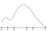
(a) $p(t)$

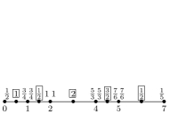
(b) B-ordinates of $p(t)$

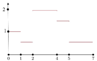
(c) $q(t)$

Figure 5: The mapping of $p(t)$.

Fig. 5(a) shows $p(t)\in\overline{\mathbf{S}}(2,1,\mathrm{T})$ on some interior intervals of $\mathrm{T}$, Fig. 5(c) shows the mapping result $q(t)\in\overline{\mathbf{S}}(0,-1,\mathrm{G})$ on the corresponding intervals. In fact, the value of $q(t)$ on each interval in Fig. 5(c) is the B-ordinate on the centre of each interval, which is shown in Fig. 5(b).

Lemma 3.5

The mapping defined in Definition 3.4 is injective.

Proof 1

Obviously, $\mathbf{\Phi}(p(t))\equiv 0$ implies $p(t)\equiv 0$ for $p(t)\in\overline{\mathbf{S}}(2,1,\mathrm{T})$. Thus, $\mathbf{\Phi}$ is injective.

From Lemma 3.5, the mapping we defined in Definition 3.4 is an injective mapping. To ensure the mapping is a bijective mapping, for each basis function of $\overline{\mathbf{S}}(0,-1,\mathrm{G})$, we need to construct a basis function of $\overline{\mathbf{S}}(2,1,\mathrm{T})$.

3.3 Construction of the basis functions for $\overline{\mathbf{S}}(2,1,\mathrm{T})$

In this subsection, we first initialize the B-ordinates of the quadratic basis function in $\overline{\mathbf{S}}(2,1,\mathrm{T})$ via the value of a basis function in $\overline{\mathbf{S}}(0,-1,\mathrm{G})$, and then give an algorithm to calculate the B-ordinates of the quadratic basis function.

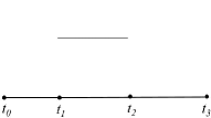
(a) $q(t)$

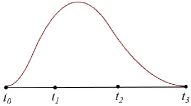
(b) $p(t)$

Figure 6: The inverse mapping.

Figure 7: The B-ordinates $b^{i}_{j},i=0,1,2;j=0,1,2$ of $p(t)$.

Given the basis function of $\overline{\mathbf{S}}(0,-1,\mathrm{G})$ in Fig. 6(a):

$$q(t)=\begin{cases}1,&[t_{1},t_{2}]\\ 0,&\text{other intervals}.\end{cases}$$ (14)

With Equation (14), we initialize the B-ordinates of $p(t)\in\overline{\mathbf{S}}(2,1,\mathrm{T})$ as:

$$b^{i}_{1}=\begin{cases}1,&i=1\\ 0,&i\neq 1\end{cases},$$ (15)

which are the B-ordinates on “$\color[rgb]{0,1,0}{{\bullet}}$” in Fig. 7. Obviously, the support of $p(t)$ is $[t_{0},t_{3}]$. To calculate all of the B-ordinates $b^{i}_{j},i=0,1,2;j=0,2$ for the polynomial function $p(t)\in\overline{\mathbf{S}}(2,1,\mathrm{T})$ we give some conclusions as follows:

Proposition 3.6

We use Fig.7 to illustrate some conclusions as follows:

1. $p(t)$ is $C^{1}$ continuous on $t_{1}$ if and only if $(t_{1},b^{0}_{2})$ occupies on the linear function that determinated by $(\frac{t_{0}+t_{1}}{2},b^{0}_{1})$ and $(\frac{t_{1}+t_{2}}{2},b^{1}_{1})$.

2. $p(t)$ is $C^{1}$ continuous on $t_{2}$ if and only if $(t_{2},b^{1}_{2})$ occupies on the linear function that determinated by $(\frac{t_{1}+t_{2}}{2},b^{1}_{1})$ and $(\frac{t_{2}+t_{3}}{2},b^{2}_{1})$.

Proof 2

1. As $p(t)$ is $C^{1}$ continuous on $t_{1}$, we obtain $b^{1}_{0}=b^{0}_{2}$ and

$$\frac{b^{0}_{2}-b^{0}_{1}}{t_{1}-t_{0}}=\frac{b^{1}_{1}-b^{0}_{2}}{t_{2}-t_{1}},$$ (16)

with Equation (16), we obtain

$$\frac{b^{0}_{2}-b^{0}_{1}}{b^{1}_{1}-b^{0}_{1}}=\frac{t_{1}-\frac{t_{1}+t_{0}}{2}}{\frac{t_{2}+t_{1}}{2}-\frac{t_{1}+t_{0}}{2}},$$ (17)

with Equation (17), the point$(t_{1},b^{0}_{2})$ is on the linear function that is determined by the points $(\frac{t_{0}+t_{1}}{2},b^{0}_{1})$ and $(\frac{t_{1}+t_{2}}{2},b^{1}_{1})$.

The reverse proving process can be derived naturally.

2. Similar to 1, the proposition is correct.

Input: The support $[t_{0},t_{1},t_{2},t_{3}]$; $b^{0}_{1},b^{1}_{1},b^{2}_{1}$.

Output: All of the B-ordinates of $p(t)$ on $[t_{0},t_{3}]$ in Fig. 7.

1Using the two points $(\frac{t_{0}+t_{1}}{2},0)$ and $(\frac{t_{1}+t_{2}}{2},1)$ to calculate the linear function on $(t_{1},b^{0}_{2})$;

2 Calculate the B-ordinate on $t_{1}$ as $b^{0}_{2}=\frac{t_{1}-t_{0}}{t_{2}-t_{0}}$;

3 Using the two points $(\frac{t_{1}+t_{2}}{2},1)$ and $(\frac{t_{2}+t_{3}}{2},0)$ to calculate the linear function on $(t_{2},b^{2}_{0})$;

4 Calculate the B-ordinate on $t_{2}$ as $b^{2}_{0}=\frac{t_{2}-t_{1}}{t_{1}-t_{3}}+1$;

5 Obtain the B-ordinates on $[t_{1},t_{2}]$ as $\{b^{0}_{2},1,b^{2}_{0}\}$;

6 Using the $C^{1}$ continuous condition to calculate that the B-ordinates on $t_{0}$ and$\frac{t_{0}+t_{1}}{2}$ are 0;

7 Obtain the B-ordinates on $[t_{0},t_{1}]$ as $\{0,0,b^{0}_{2}\}$;

8 Using the $C^{1}$ continuous condition to calculate that the B-ordinates on $\frac{t_{2}+t_{3}}{2}$ and $t_{3}$ are 0;

9 Obtain the B-ordinates on $[t_{2},t_{3}]$ as $\{b^{2}_{0},0,0\}$;

Algorithm 1 Calculate the B-ordinates of $p(t)\in\mathbf{S}(2,1,\mathrm{T})$

Then, given the B-ordinates by Equation (15), we can calculate the B-ordinates of $p(t)\in\overline{\mathbf{S}}(2,1,\mathrm{T})$ via Algorithm 1. We show $p(t)$ in Fig. 6(b), $p(t)$ is $C^{1}$ continuous, and $p(t)=\mathbf{\Phi}^{-1}(q(t))$.

3.4 The isomorphic univariate spaces and properties

In this subsection, we prove that the mapping is bijective, $\overline{\mathbf{S}}(2,1,\mathrm{T})$ is isomorphic to $\overline{\mathbf{S}}(0,-1,\mathrm{G})$, the basis functions of $\overline{\mathbf{S}}(2,1,\mathrm{T})$ hold the properties of are linearly independence, partition of unity and completeness.

Theorem 3.7

The mapping defined in definition 3.4 holds the property of bijectivity.

Proof 3

For each basis function of $\overline{\mathbf{S}}(0,-1,\mathrm{G})$, we can obtain a quadratic function of $\overline{\mathbf{S}}(2,1,\mathrm{T})$ via Algorithm 1, the mapping is surjective. As the mapping is injective, the mapping holds the property of bijectivity.

As the mapping between $\overline{\mathbf{S}}(2,1,\mathrm{T})$ and $\overline{\mathbf{S}}(0,-1,\mathrm{G})$ is bijective. We obtain the following corollary naturally.

Corollary 3.8

$\overline{\mathbf{S}}(2,1,\mathrm{T})$ is isomorphic to $\overline{\mathbf{S}}(0,-1,\mathrm{G})$.

Theorem 3.9

The basis functions of $\mathbf{S}(2,1,\mathrm{T})$, which are constructed in 3.3, hold the properties of linearly independence, partition of unity and completeness on $[t_{0},t_{n}]$.

Proof 4

Assume that the basis functions of $\overline{\mathbf{S}}(0,-1,\mathrm{G}^{\varepsilon})$ are $q_{i}(t)$, the basis functions of $\overline{\mathbf{S}}(2,1,\mathrm{T}^{\varepsilon})$ are $p_{i}(t),i=1,...,N$, where $\mathrm{G}^{\varepsilon}$ is the C-knots of $\mathrm{T}^{\varepsilon}$. We obtain that the mapping between $\overline{\mathbf{S}}(2,1,\mathrm{T}^{\varepsilon})$ and $\mathbf{S}(0,-1,\mathrm{G}^{\varepsilon})$ is bijective, and $\overline{\mathbf{S}}(2,1,\mathrm{T}^{\varepsilon})$ is isomorphic to $\overline{\mathbf{S}}(0,-1,\mathrm{G}^{\varepsilon})$.

As the spaces are linear spaces and $\mathbf{\Phi}^{-1}(q_{i}(t))=p_{i}(t)$, we obtain

$$\sum^{N}_{i=1}p_{i}(t)=\sum^{N}_{i=1}\mathbf{\Phi}^{-1}(q_{i}(t))=\mathbf{\Phi}^{-1}(\sum^{N}_{i=1}q_{i}(t)).$$

As $\sum^{N}_{i=1}(q_{i}(t))=1,t\in[t_{-1},t_{n+1}],$ the B-ordinate on the centre position of each interior interval on $\mathrm{T}^{\varepsilon}$ are $1$. By Algorithm 1, the B-ordinates on each interval of $\mathrm{T}$ is $1$. With Equation (10) and Equation (11), the basis functions of $\mathbf{S}(2,1,\mathrm{T})$ have partition of unity on $[t_{0},t_{n}]$.

As the basis functions of $\overline{\mathbf{S}}(0,-1,\mathrm{G}^{\varepsilon})$ are linearly independent and complete on $[t_{0},t_{n}]$, and $\overline{\mathbf{S}}(2,1,\mathrm{T}^{\varepsilon})$ is isomorphic to $\overline{\mathbf{S}}(0,-1,\mathrm{G}^{\varepsilon})$, the polynomial functions of $\overline{\mathbf{S}}(2,1,\mathrm{T}^{\varepsilon})$ are linearly independent and complete on $[t_{0},t_{n}]$. With Equation (10) and Equation (11), the basis functions of $\mathbf{S}(2,1,\mathrm{T})$, which are constructed in 3.3, are linearly independent and complete on $[t_{0},t_{n}]$. The theorem is proved.

Till now, we construct a bijective mapping between $\overline{\mathbf{S}}(2,1,\mathrm{T})$ and $\overline{\mathbf{S}}(0,-1,\mathrm{G})$, the two spaces are isomorphic to each other, some important properties are the same for the basis functions of the two spaces. For $\mathbf{S}(2,2,1,1,\mathscr{T})$, we want to obtain similar conclusions. We denote $\mathbf{S}(d,d,d-1,d-1,\mathscr{T})$ as $\mathbf{S}^{d}(\mathscr{T})$ for convenience. By Equation 7, we first discuss the spline space $\mathbf{S}^{2}(\mathscr{T})$ with homogeneous boundary conditions, which is denoted by $\overline{\mathbf{S}}^{2}(\mathscr{T})$.

4 The mapping between $\overline{\mathbf{S}}^{2}(\mathscr{T})$ and $\overline{\mathbf{S}}^{0}(\mathscr{G})$

In this section, we will introduce the mapping between $\overline{\mathbf{S}}^{2}(\mathscr{T})$ and $\overline{\mathbf{S}}^{0}(\mathscr{G})$.

4.1 Some notations and CVR graphs

Before we give the mapping, we introduce some notations for a hierarchical T-mesh in Table 1, we also give some abbreviations in brackets for convenience.

Notations		Definitions
P-cell($\mathcal{PC}$)		An interior-cell that four corner vertices are crossing-vertices.
T-cell		An interior-cell that at least one of four corner vertices is a T-junction.
T-connected		Two T-cells are T-connected if they connect at a T-junction.
T-connection($\mathcal{TC}$)		The union of all T-connected T-cells.
P-domain($\mathcal{PD}$)		The domain on which a pure-cell occupies.
T-connection-domain($\mathcal{TCD}$)		The domain on which a T-connection occupies.
T-rectangle-domain($\mathcal{TRD}$)		The minimal rectangular domain that covers a T-connection.
Domain($\mathcal{D}$)		The minimal rectangular domain that covers a T-connection.
Domain-center		The centre point of the domain.
One-neighbour-cell		The lowest level cells adjacent to the T-connection.
The level of the T-connection		The level of the one-neighbour-cells corresponds to the T-connection.

Table 1: Some notations for hierarchical T-meshes

(a) $\mathscr{T}$	(b) $\mathscr{G}$

Figure 8: Notations and CVR graph.

We use Fig. 8(a) to introduce the notations in Table 1. In Fig. 8(a), cell $0$ and cell $5$ are P-cells, while cell $1$, cell $2$ and cell $3$ are T-cells. Cell $1$ and cell $2$ are T-connected, cell $2$ and cell $3$ are T-connected. The T-connection, which can be denoted as $\mathcal{TC}_{0}$, is the union that consists of cell $1$, cell $2$ and cell $3$. As cell $5$ is a P-cell, the gray domain is a P-domain. The green domain is the T-connection-domain of $\mathcal{TC}_{0}$, the domain inside the red square is the T-rectangle-domain of $\mathcal{TC}_{0}$, the domain-centre of the T-rectangle-domain is denoted as $``{\bullet}"$ in Fig. 8(a). Cell $4$ is the one-neighbour-cell of $\mathcal{TC}_{0}$, the level of cell $4$ is the level of $\mathcal{TC}_{0}$.

In [23], Definition 4.10 is introduced to propose a topological explanation to the dimension formula of $\mathbf{S}(2,2,1,1,\mathscr{T})$.

Definition 4.10

[23] Given a hierarchical T-mesh $\mathscr{T}$, we can construct a graph $\mathscr{G}$ by retaining the crossing-vertices and the line segments with two end points that are crossing-vertices and removing the other vertices and the edges in $\mathscr{T}$. $\mathscr{G}$ is called the crossing-vertex-relationship graph (CVR graph for short) of $\mathscr{T}$.

We introduce some notations of CVR graph for the mapping in Table 2, we also give some abbreviations in brackets for convenience.

Notations		Definitions
g-cell ($\mathcal{GC}$)		A grid element in CVR graph.
P-g-cell ($\mathcal{PGC}$)		A g-cell corresponds to a P-cell in $\mathscr{T}$.
T-g-cell ($\mathcal{TGC}$)		A g-cell corresponds to a T-connection-domain in $\mathscr{T}$.

Table 2: Cells for CVR graphs

We also use Fig. 8 to illustrate the notations in Table 2. Fig. 8(b) shows the CVR graph $\mathscr{G}$ of the hierarchical T-mesh $\mathscr{T}$ in Fig. 8(a). The P-cell 0 in 8(a) corresponds to the P-g-cell 0 in 8(b). In Fig. 8(a), for the T-connection $\mathcal{TC}_{0}$, the T-connection-domain of $\mathcal{TC}_{0}$ corresponds to the T-g-cell 1 in Fig. 8(b).

From the relationship between the cells of a hierarchical T-mesh and its CVR graph, we consider the mapping between $\overline{\mathbf{S}}^{2}(\mathscr{T})$ and $\overline{\mathbf{S}}^{0}(\mathscr{G})$.

4.2 The mapping formulae between $\overline{\mathbf{S}}^{2}(\mathscr{T})$ and $\overline{\mathbf{S}}^{0}(\mathscr{G})$

By the notations in Table 1 and Table 2, we use the B-ordinates to define a functional, and then use the functional to construct the mapping between $\overline{\mathbf{S}}^{2}(\mathscr{T})$ and $\overline{\mathbf{S}}^{0}(\mathscr{G})$.

For the Bernstein polynomials $B^{2}_{j}(u)B^{2}_{k}(v),j,k=0,1,2$ on $[x_{0},x_{1}]\times[y_{0},y_{1}]$, where $u=\left(\frac{x-x_{0}}{x_{1}-x_{0}}\right),v=\left(\frac{y-y_{0}}{y_{1}-y_{0}}\right)$, we obtain

$$B^{2}_{1}(u)B^{2}_{1}(v)=1-\sum_{j=0}^{2}B^{2}_{j}(u)B^{2}_{0}(v)-\sum_{j=0,j\neq 1}^{2}B^{2}_{j}(u)B^{2}_{1}(v)-\sum_{j=0}^{2}B^{2}_{j}(u)B^{2}_{2}(v).$$ (18)

As $B^{2}_{j}(u),j=0,2$ possess the factors $(x-x_{0})^{2}$ or $(x-x_{1})^{2}$, and $B^{2}_{k}(v),k=0,2$ possess the factors $(y-y_{0})^{2}$ or $(y-y_{1})^{2}$. We can give the functional as follows:

Definition 4.11

Given $f(x,y)\in\overline{\mathbf{S}}^{2}(\mathscr{T})$, and $\mathcal{D}:=[x_{0},x_{1}]\times[y_{0},y_{1}]$ is a rectangular domain. Let $u=\frac{x-x_{0}}{x_{1}-x_{0}},v=\frac{y-y_{0}}{y_{1}-y_{0}}$, $f(x,y)$ can be expressed as:

$$f(x,y)=\sum_{j=0}^{2}\sum_{k=0}^{2}b_{j,k}B^{2}_{j}(u)B^{2}_{k}(v),$$

we obtain

$$f(x,y)=b_{1,1}+\sum_{j=0}^{2}(b_{j,0}-b_{1,1})B^{2}_{j}(u)B^{2}_{0}(v)+\sum_{j=0,j\neq 1}^{2}(b_{j,1}-b_{1,1})B^{2}_{j}(u)B^{2}_{1}(v)+\sum_{j=0}^{2}(b_{j,2}-b_{1,1})B^{2}_{j}(u)B^{2}_{2}(v).$$

We define a mapping functional $\mathbf{\varphi}$,

$$\mathbf{\varphi}(f(x,y):\mathcal{D})=b_{1,1}|_{\mathcal{D}},$$

where $b_{1,1}|_{D}$ denotes a piecewise constant function whose value is $b_{1,1}$ on $\mathcal{D}$.

(a) Two P-cells	(b) A T-connection

Figure 9: Two P-cells and a T-connection.

In Fig. 9(a), $C_{0}$ and $C_{1}$ are two aligned P-cells in $\mathscr{T}$. $P^{i}_{11}$ is the center domain point of $C_{i},i=0,1$. Let $f_{i}(x,y)$ be the polynomial with bi-degree $(2,2)$ defined over $C_{i}$, the B-ordinate on $P^{i}_{11}$ is denoted as $b^{i}_{11}$, the domain that covers $C_{i}$ is denoted as $\mathcal{PD}_{i},i=0,1$. Applying the functional $\varphi$ in Definition 4.11, $\mathbf{\varphi}(f_{i}(x,y):{\mathcal{PD}_{i}})=b^{i}_{1,1}|_{\mathcal{PD}_{i}},i=0,1.$

In Fig. 9(b), $C_{0}$ is the one-neighbor-cell of $\mathcal{TC}$ in $\mathscr{T}$, the T-rectangle-domain of $\mathcal{TC}$ is denoted as $\mathcal{TRD}$. Let $f_{i}(x,y)$ be the polynomial with bi-degree $(2,2)$ defined over $C_{i},i=0,...,k$,

$f_{1}(x,y)=f_{0}(x,y)+(x-x_{1})^{2}v(y),$

$f_{2}(x,y)=f_{0}(x,y)+(x-x_{1})^{2}v(y)+c_{1}(x-x_{1})^{2}(y-y_{1})^{2},$

$\vdots$

$f_{k}(x,y)=f_{0}(x,y)+(x-x_{1})^{2}v(y)+c_{1}(x-x_{1})^{2}(y-y_{1})^{2}+...+c_{k-1}(x-x_{1})^{2}(y-y_{k_{1}})^{2},v(y)\in\mathbb{P}_{2}(y),c_{i}\in\mathbb{R}.$

As $f_{i}(x,y),i=1,...,k$ possess the cofactor $(x-x_{1})^{2}$, $\mathbf{\varphi}(f_{i}(x,y):{\mathcal{TRD}})=\mathbf{\varphi}(f_{0}(x,y):{\mathcal{TRD}})$.

Given a hierarchical T-mesh $\mathscr{T}$, $\mathscr{G}$ denotes the CVR graph of $\mathscr{T}$. For $f(x,y)\in\overline{\mathbf{S}}^{2}(\mathscr{T})$, we denote the support of $f(x,y)$ as $Sup(f)$. From Table 1 and Table 2, $\mathcal{PC}$ is denoted as a P-cell of $Sup(f)$, the P-domain of $\mathcal{PC}$ is denoted as $\mathcal{PD}$, the P-g-cell corresponds to $\mathcal{PC}$ in $\mathscr{G}$ is denoted as $\mathcal{PGC}$; $\mathcal{TC}$ is denoted as a T-connection of $Sup(f)$, the T-rectangle-domain of $\mathcal{TC}$ is denoted as $\mathcal{TRD}$. And the T-g-cell corresponds to $\mathcal{TC}$ in $\mathscr{G}$ is denoted as $\mathcal{TGC}$. We can define the mapping between $\overline{\mathbf{S}}^{2}(\mathscr{T})$ and $\overline{\mathbf{S}}^{0}(\mathscr{G})$ as follows:

Definition 4.12

The mapping formulae between $\overline{\mathbf{S}}^{2}(\mathscr{T})$ and $\overline{\mathbf{S}}^{0}(\mathscr{G})$ is defined as :

$$\mathbf{\Phi}:\overline{\mathbf{S}}^{2}(\mathscr{T})\rightarrow\overline{\mathbf{S}}^{0}(\mathscr{G}),$$ (19)

$$\begin{cases}\mathbf{\varphi}(f(x,y)|_{\mathcal{PC}}:{\mathcal{PD}})\to g(x,y)|_{\mathcal{PGC}}\\ \mathbf{\varphi}(f(x,y)|_{\mathcal{TC}}:{\mathcal{TRD}})\to g(x,y)|_{\mathcal{TGC}}.\end{cases}$$ (20)

Where $f(x,y)\in\overline{\mathbf{S}}^{2}(\mathscr{T})$, $f(x,y)|_{\mathcal{PC}}$ denotes the expression of $f(x,y)$ on $\mathcal{PC}$, $g(x,y)\in\overline{\mathbf{S}}^{0}(\mathscr{G})$, and $g(x,y)|_{\mathcal{PGC}}$ denotes the expression of $g(x,y)$ on $\mathcal{PGC}$, which corresponds to $\mathcal{PC}$; $f(x,y)|_{\mathcal{TC}}$ denotes the expression of $f(x,y)$ on the one-neighbour-cell of $\mathcal{TC}$, and $g(x,y)|_{\mathcal{TGC}}$ denotes the expression of $g(x,y)$ on $\mathcal{TGC}$, which corresponds to $\mathcal{TC}$.

4.3 The injectivity property of the mapping

(a)	(b)	(c)

Figure 10: Figures for Lemma 4.13.

Lemma 4.13

Given a hierarchical T-mesh $\mathscr{T}$, for each T-connection $\mathcal{TC}\in\mathscr{T}$, the T-rectangle-domain of $\mathcal{TC}$ is denoted as $\mathcal{TRD}$. At least one one-neighbour-cell of $\mathcal{TC}$ exists, and for all the one-neighbour-cells of $\mathcal{TC}$, apply the functional $\mathbf{\varphi}$ with the polynomial of each one-neighbour-cell on $\mathcal{TRD}$, the results are the same.

Proof 5

Without loss of generality, we use Fig. 10 to illustrate the lemma.

1. At least one one-neighbour-cell of $\mathcal{TC}$ exists.

In Fig. 10(a), we denote the level of $C_{i}$ as $l_{i}$ ,where $i=0,1,2,3$. As $v_{0}$ is a T-junction, we get $l_{2}\leqslant l_{0}$ and $l_{2}\leqslant l_{1}$. As $v_{1}$ is a T-junction, we get $l_{3}\leqslant l_{2}$. Then, $C_{3}$ is the cell with the lowest level of $C_{0},C_{1},C_{2},C_{3}$. In a similar manner, one-neighbour-cell must exist.

2. If at least two one-neighbour-cells of $\mathcal{TC}$ exist, they are connected to $\mathcal{TC}$ and have the same level.

According to Fig. 10 (b), the neighbour cells of $\mathcal{TC}$ are $C_{1},C_{2},C_{3}$ and $C_{4}$. The maximum level of the cells in $\mathcal{TC}$ is $l_{0}$, and the level of $C_{i}$ is $l_{i}$, where $i=1,2,3,4$. As the mesh is a hierarchical T-mesh, we can assume $l_{1}=l_{3}=l$, and by (1), $l<l_{0}$ .

(1) Assume $l_{2}>l$, then $l_{4}<l$.

We use proofs by contradiction to prove $l_{4}<l$. If $l_{4}>l$, by the assumption, $l_{2}>l$, then $\mathcal{TC}$ will be divided, and we obtain a contradiction. Thus, $l_{4}<l$ and $C_{4}$ is the only one-neighbour-cell.

(2) Assume $l_{2}<l$ and $l_{4}<l$.

If $l_{2}<l_{4}$, $C_{2}$ is the only one-neighbour-cell. If $l_{2}>l_{4}$, $C_{4}$ is the only one-neighbour-cell. If $l_{2}=l_{4}$, $C_{2}$ and $C_{4}$ are connected to $\mathcal{TC}$.

Thus, if $\mathcal{TC}$ has at least two one-neighbour-cells, the levels of the one-neighbour-cells are same.

3. The one-neighbour-cell is aligned with $\mathcal{TC}$ .

According to Fig. 10 (c), $v_{0}$ must be cross-vertexes; otherwise, the one-neighbour-cell of $\mathcal{TC}$ is not the lowest level cell.

From the above, the mapping is well defined and the mapping result is unique. The lemma is proved.

Theorem 4.14

The mapping defined in Equation (19) is injective.

Proof 6

By Lemma 4.13, the mapping result on each T-connection is unique, and $\mathbf{\Phi}(f(x,y))\equiv 0$ implies $f(x,y)\equiv 0$ for $f(x,y)\in\overline{\mathbf{S}}^{2}(\mathscr{T})$. Thus, $\mathbf{\Phi}$ is injective.

The mapping we defined in Definition 4.12 is injective. To verify that the mapping is a bijective mapping, we need to confirm the mapping is surjective. In other words, given a basis function $q(x,y)\in\overline{\mathbf{S}}^{0}(\mathscr{G})$, we need to construct the corresponding basis function $p(x,y)\in\overline{\mathbf{S}}^{2}(\mathscr{T})$, and $p(x,y)$ is the inverse image of $q(x,y)$.

5 Construction of the basis functions for $\overline{\mathbf{S}}^{2}(\mathscr{T})$

In this section, we give a general method to construct the basis functions of $\overline{\mathbf{S}}^{2}(\mathscr{T})$ when there is no limitation for level difference on $\mathscr{T}$. Each basis function corresponds to a basis function of $\overline{\mathbf{S}}^{0}(\mathscr{G})$. First, we propose a new structure and introduce how to use T-structures for calculating the B-ordinates. Second, for each basis function of $\overline{\mathbf{S}}^{2}(\mathscr{T})$, we initialize the weights on each domain of $\mathscr{T}$ via the basis function of $\overline{\mathbf{S}}^{0}(\mathscr{G})$, we use the T-structures to calculate the B-ordinates for the basis function of $\overline{\mathbf{S}}^{2}(\mathscr{T})$. Finally, we propose that our computation can be reduced by simplifying $\mathscr{T}$.

5.1 T-structures and some conclusions for T-structures

T-structures will play an important role in calculating the B-ordinates for each basis function of $\overline{\mathbf{S}}^{2}(\mathscr{T})$. In this subsection, we introduce how to use T-structures for calculating the B-ordinates of a polynomial function on the T-structure.

5.1.1 Some notations for T-structures

Figure 11: The T-structure $\mathcal{T}$.

Definition 5.15

In the hierarchical T-mesh $\mathscr{T}$, a c-edge and all of the cells that have at least one common vertex with the c-edge constitute a T-structure of $\mathscr{T}$, we denote the T-structure as $\mathcal{T}$ for convenience. The c-edge is referred to as the mid-edge of $\mathcal{T}$. All of the vertices on the c-edge are referred to as the interior-vertices of $\mathcal{T}$. The end-points of the c-edge are referred to as the end-points of $\mathcal{T}$. The lowest level cell that has the common edge with the c-edge is referred to as the mother-cell of $\mathcal{T}$. The cells adjacent to the mid-edge except the mother-cell are referred to as the sub-cells of $\mathcal{T}$. The level of the mother-cell is denoted as the level of $\mathcal{T}$. If the mid-edge is horizontal(vertical), the T-structure is referred to as a horizontal(vertical) T-structure.

In Fig. 11, the T-structure $\mathcal{T}$ consists of the c-edge $v_{0}v_{m}$ and the cells $C_{0},...,C_{n}$. $v_{0}v_{m}$ is the mid-edge of $\mathcal{T}$. $v_{0},...,v_{m}$ are the interior-vertices of $\mathcal{T}$. $v_{0}$ and $v_{m}$ are the end-points of $\mathcal{T}$. $C_{0}$ is the mother-cell of $\mathcal{T}$. $C_{5},...,C_{n}$ are the sub-cells of $\mathcal{T}$. The level of the mother-cell $C_{0}$ is the level of the T-structure $\mathcal{T}$. $\mathcal{T}$ is a horizontal T-structure.

(a) T-structures	(b) A T-structure-branch

Figure 12: T-structures on a hierarchical T-mesh .

Definition 5.16

One horizontal T-structure and one vertical T-structure are connected if they have one common interior-vertex. The union of all connected T-structures is referred to as a T-structure-branch, which is denoted as $\mathcal{TSB}$. The minimal level of the T-structures in a T-structure-branch is denoted as the level of the T-structure-branch.

We show an example in Fig. 12: $\mathcal{T}_{0}$ in Fig. 12 (b) consists of the c-edge $v_{0}v_{2}$ and the surrounding cells $0,1,...,7$, which are shown in Fig. 12 (a); $\mathcal{T}_{1}$ in Fig. 12 (b) consists of the c-edge $v_{1}v_{3}$ and the surrounding cells $0,4,5,8,9,{10}$, which are shown in Fig. 12 (a); and $\mathcal{T}_{2}$ in Fig. 12 (b) consists of the c-edge $v_{3}v_{4}$ and the surrounding cells $5,8,9,...,{13}$, which are shown in Fig. 12 (a). $\mathcal{T}_{0}$ and $\mathcal{T}_{1}$ are connected at $v_{1}$, $\mathcal{T}_{1}$ and $\mathcal{T}_{2}$ are connected at $v_{3}$. In Fig. 12(b), $\mathcal{T}_{0},\mathcal{T}_{1}$ and $\mathcal{T}_{2}$ constitute a T-structure-branch. In Fig. 12(b), the level of $\mathcal{T}_{0}$ is denoted as the level of the T-structure-branch.

To make use of the T-structure-branches in Definition 5.16, we give a lemma to connect the T-structure-branches with T-connections.

Lemma 5.17

Given the T-connection $\mathcal{TC}\in\mathscr{T}$, $\mathcal{TC}$ will be covered by a T-structure-branch.

Proof 7

Assume $\mathcal{T}_{1},\mathcal{T}_{2},...,\mathcal{T}_{n}$ are the T-structures that cover the T-cells $\{C_{1},C_{2},...,C_{m}\}$.

1. When $m=1$, obviously, only one T-structure $T_{1}$ covers $\mathcal{TC}$. The conclusion is right.

2. When $m>1$, we prove it by reduction to absurdity.

   Without loss of generality, assume $\mathcal{T}_{1}$ is not connected with any T-structure of $\mathcal{T}_{2},\mathcal{T}_{3},...,\mathcal{T}_{n}$. Assume that the sub-cells of $\mathcal{T}_{0}$ are $I=\{C_{i_{1}},...,C_{i_{k}}\}$, and $\{i_{1},...,i_{k}\}$ is a sub set of $\{1,...,m\}$. We denote $\{C_{1},C_{2},...,C_{m}\}\setminus I$ as the sub T-cell set of $\{C_{1},C_{2},...,C_{m}\}$ except $\{C_{i_{1}},...,C_{i_{k}}\}$. T-cells in $\{C_{1},C_{2},...,C_{m}\}\setminus I$ are not T-connected to the T-cells in $I$, and $\mathcal{TC}$ will be divided into two, it is a contradiction of the assumption. Thus, T-structures $\mathcal{T}_{1},\mathcal{T}_{2},...,\mathcal{T}_{n}$ comprise a T-structure-branch.

The lemma is proved.

We also show an example by Fig. 12: In Fig. 12(a), the T-connection $\mathcal{TC}$ consists of cell 3, cell 4, cell 5, cell 8, cell 11; in Fig. 12(b), the T-structure Branch $\mathcal{TSB}$ consists of $\mathcal{T}_{0}$,$\mathcal{T}_{1}$ and $\mathcal{T}_{2}$; obviously, the cells of $\mathcal{TC}$ are covered by the cells belonging to $\mathcal{TSB}$.

5.1.2 B-net method on T-structures

In order to connect T-structures with B-ordinates, we introduce the B-net method on T-structures as follows.

(a) The end points are two crossing-vertices	(b) One of the end-pint is a crossing-vertex

Figure 13: The corresponding B-ordinates on T-structures

Let $p(x,y)\in\overline{\mathbf{S}}^{2}(\mathscr{T})$ be the polynomial defined over the cells of the T-structure $\mathcal{T}\in\mathscr{T}$. We assume $\mathcal{T}$ as a horizontal T-structure in Fig. 13(a), we refer to the B-ordinates on “$\color[rgb]{0,1,0}{\bullet}$”, “${\bullet}$” and “$\circ$” as the corresponding B-ordinates of $p(x,y)$ on $\mathcal{T}$. For the T-structure in Fig. 13(b), the corresponding B-ordinates can be defined similarly. For the vertical T-structures, we can also define the notations similarly.

Lemma 5.18

For a T-structure $\mathcal{T}\in\mathscr{T}$, let $p(x,y)\in\overline{\mathbf{S}}^{2}(\mathscr{T})$ be the polynomial defined over the cells of $\mathcal{T}$. Then, when the two rows (columns) B-ordinates on the mother-cell that near the mid-edge are given, the two rows (columns) B-ordinates on sub-cells that near the mid-edge are determined.

Proof 8

We prove the lemma for horizonal T-structures. In Fig. 13, when the B-ordinates on “$\circ$” of the mother-cell are given, the B-ordinates on “$\color[rgb]{0,1,0}{\bullet}$” of the sub-cells can be calculated via B-net method. If it is a vertical T-structure, the lemma can be similarly proved.

By Lemma 5.18, if we want to obtain the two rows (column) B-ordinates of sub-cells that are near the mid-edge, we need to obtain the six B-ordinates of the mother-cell that are near the mid-edge.

5.1.3 The corresponding B-ordinates on a crossing-vertex

In this subsection, we introduce the B-ordinates associated with a crossing-vertex, which can help us to obtain the six B-ordinates of the mother-cell that are near the mid-edge.

Let $p(x,y)\in\overline{\mathbf{S}}^{2}(\mathscr{T})$ be the polynomial defined over the cells around a crossing-vertex $v^{+}\in\mathscr{T}$, which are shown in Fig. 14(a). We define the sixteen B-ordinates on the green domain points in Fig. 14(a) as the corresponding B-ordinates of $p(x,y)$ on $v^{+}$. In Fig. 14, the crossing-vertex $v^{+}$ is denoted as “${\blacksquare}$”, the cells around $v^{+}$ are denoted as $C_{i}$, where $i=1,2,3,4$, and $C_{1}$ is denoted as the cell with the top level. We use Fig. 14 to give the lemma that describes the relationship between the corresponding B-ordinates on a crossing-vertex and the bilinear function as follows:

(a)	(b)

Figure 14: Corresponding B-ordinates around a crossing-vertex.

Lemma 5.19

For each crossing-vertex $v^{+}\in\mathscr{T}$, the corresponding B-ordinates of $p(x,y)\in\overline{\mathbf{S}}^{2}(\mathscr{T})$ on $v^{+}$ are on a bilinear function.

Proof 9

We also use Fig. 14 to illustrate the proving process. In Fig. 14(a), the domain points of $C_{1}$ around $v^{+}$ are $P^{1}_{j,k}=(s^{1}_{j,k},t^{1}_{j,k})$, where $j,k=1,2$, which are denoted as “$\color[rgb]{0,1,0}{\bullet}$” on $C_{1}$. The bilinear function $f_{1}(s,t)=a_{1}st+b_{1}s+c_{1}t+d_{1}$, where $j,k=1,2$, which satisfies $f_{1}(s^{1}_{j,k},t^{1}_{j,k})=b^{1}_{j,k}$, exists. Similarly, the domain points of $C_{i}$ around $v^{+}$ are denoted as “$\color[rgb]{0,1,0}\bullet$” on $C_{i}$, where $i=2,3,4$, respectively, and the corresponding bilinear functions are denoted as $f_{i}(s,t)=a_{i}st+b_{i}s+c_{i}t+d_{i}$, where $i=2,3,4$, respectively.

We use Fig. 14(b) to illustrate $f_{1}=f_{2}=f_{3}=f_{4}$. Apply the $C^{2}$ continuous conditions to $C_{i}$, where $i=2,3,4$. The B-ordinates on “$\bullet$” and the B-ordinates on “$\color[rgb]{0,1,0}\bullet$” belong to $C_{i}$ are on a common bilinear functions $f_{i}(s,t)$, where $i=2,3,4$, respectively. In Fig. 14(b), use the $C^{1}$ continuous condition of $C_{1}$ and $C_{2}$. The B-ordinates on “$\bullet$” of $C_{1}$ and $C_{2}$ are on a common bilinear function; thus $f_{1}=f_{2}$. Similarly, we obtain $f_{1}=f_{3},f_{2}=f_{3}$ and $f_{3}=f_{4}$; then, $f_{1}=f_{2}=f_{3}=f_{4}$. Thus, the lemma is proved.

By Lemma 5.19, if we want to calculate the corresponding B-ordinates for a crossing-vertex $v^{+}$, we need to determine the bilinear function $f(s,t)=ast+bs+ct+d$ of $v^{+}$. For $f(s,t)$, to determine $a,b,c$ and $d$, we recall the notation of the adaptive nodes [33] for a bilinear function.

5.1.4 The adaptive nodes for a bilinear funtion

We use Fig. 15 to illustrate how to obtain a group of adaptive nodes for a bilinear function.

Figure 15: Adaptive nodes for a bilinear function.

1. Choose the point $v_{1}(s_{1},t_{1})\in\mathbb{R}^{2}$.

2. Draw the cross $X_{1}$ $\in\mathbb{R}^{2}$, and $v_{1}\notin X_{1}$. Choose two points $v_{2}(s_{2},t_{2})$ and $v_{3}(s_{3},t_{3})$ on one edge of $X_{1}$, and choose another point $v_{4}(s_{4},t_{4})$ on the other edge of $X_{1}$.

$v_{1},v_{2},v_{3}$ and $v_{4}$ are referred to as adaptive nodes of the bilinear function $f(s,t)=ast+bs+ct+d$. Given the corresponding $f(s_{i},t_{i}),i=1,...,4$, we can use the linear equations $f(s_{i},t_{i})=as_{i}t_{i}+bs_{i}+ct_{i}+d,i=1,...,4$ to calculate the coefficients $a,b,c$ and $d$.

And then, we give the following lemma to illustrate the relationship between the corresponding B-ordinates and the adaptive nodes on each end-point of $\mathcal{T}$:

Theorem 5.20

Assume that the two end-points of the T-structure $\mathcal{T}\in\mathscr{T}$ are crossing-vertices. Let $p(x,y)\in\overline{\mathbf{S}}^{2}(\mathscr{T})$ be the polynomial defined over the cells of $\mathcal{T}$. Given the values on a group of adaptive nodes for each end-point of $\mathcal{T}$, the corresponding B-ordinates on $\mathcal{T}$ can be calculated by Lemma 5.18.

Proof 10

By Lemma 5.19, the corresponding B-ordinates on each end-point are on a bilinear function. For each end-point, as the value on each adaptive node is given, the coefficients of each bilinear function are calculated by four equations, the corresponding B-ordinates on each end-points can be calculated by the corresponding bilinear functions, the two rows (column) B-ordinates of the mother-cell that near the mid-edge are obtained, and the corresponding B-ordinates on $\mathcal{T}$ can be calculated by Lemma 5.18, and the corresponding B-ordinates satisfy the $C^{1}$ continuous conditions.

Till now, we obtain the conclusion that if we want to obtain the corresponding B-ordinates on a T-structure, we need to obtain a group of adaptive nodes and the corresponding values on the nodes. We use Fig. 16 to give the following proposition to discuss the values on the adaptive nodes for the end-points of a T-structure.

(a) Two P-cells	(b) A T-connection and the corresponding one-neighbor-cell

Figure 16: The nodes can be used in hierarchical T-mesh

In Fig. 16(a), $C_{0}$ and $C_{1}$ are two aligned P-cells in $\mathscr{T}$. $P^{0}_{01}(x_{1},\frac{y_{0}+y_{k}}{2})$ and $P^{0}_{11}(\frac{x_{1}+x_{2}}{2},\frac{y_{0}+y_{k}}{2})$ are two domain-points of $C_{0}$. $P^{1}_{11}(\frac{x_{0}+x_{1}}{2},\frac{y_{0}+y_{k}}{2})$ and $P^{1}_{21}(x_{1},\frac{y_{0}+y_{k}}{2})$ are two domain-points of $C_{1}$. Let $p_{i}(x,y)\in\overline{\mathbf{S}}^{2}(\mathscr{T})$ be the polynomial defined over $C_{i},i=0,1$. The B-ordinate of $p_{0}(x,y)$ on $P^{0}_{i1}$ is denoted as $b^{0}_{i1},i=0,1$. The B-ordinate of $p_{1}(x,y)$ on $P^{1}_{i1}$ is denoted as $b^{1}_{i1},i=1,2$.

In Fig. 16(b), $C_{0}$ is the one-neighbor-cell of $\mathcal{TC}$ in $\mathscr{T}$, the T-connection-domain of $\mathcal{TC}$ is denoted as $\mathcal{TCD}$, the T-rectangle-domain of $\mathcal{TC}$ is denoted as $\mathcal{TRD}$. Let $p_{i}(x,y)\in\overline{\mathbf{S}}^{2}(\mathscr{T})$ be the polynomial defined over $C_{i},i=0,..,k$, $\mathbf{\varphi}(p_{i}(x,y):{\mathcal{TRD}})=\mathbf{\varphi}(p_{0}(x,y):{\mathcal{TRD}})=\omega|_{\mathcal{TCD}}$. The center position of $\mathcal{TRD}$ is denoted as $P(\frac{x_{0}+x_{1}}{2},\frac{y_{0}+y_{k}}{2})$. $P^{0}_{01}(x_{1},\frac{y_{0}+y_{k}}{2})$ and $P^{0}_{11}(\frac{x_{1}+x_{2}}{2},\frac{y_{0}+y_{k}}{2})$ are denoted as two domain-points of $C_{0}$, the B-ordinate on $P^{0}_{i1}$ is denoted as $b^{0}_{i1},i=0,1$.

Proposition 5.21

From the illustrations of Fig. 16, we give the conclusions as follows:

1. In Fig. 16(a), $p(x,y)$ is $C^{1}$ continuous on $v_{1}v_{2}$ if and only if $(x_{1},\frac{y_{0}+y_{k}}{2},b^{1}_{21})$ is on the linear function that is determinated by $(\frac{x_{0}+x_{1}}{2},\frac{y_{0}+y_{k}}{2},b^{1}_{11})$ and $(\frac{x_{1}+x_{2}}{2},\frac{y_{0}+y_{k}}{2},b^{0}_{11})$.

2. In Fig. 16(b), $p(x,y)$ is $C^{1}$ continuous on $v_{1}v_{2}$ if and only if $(x_{1},\frac{y_{0}+y_{1}}{2},b^{0}_{10})$ is on the linear function that is determinated by $(\frac{x_{0}+x_{1}}{2},\frac{y_{0}+y_{k}}{2},\omega)$ and $(\frac{x_{1}+x_{2}}{2},\frac{y_{0}+y_{k}}{2},b^{0}_{11})$.

Proof 11

1. Similar to Proposition 3.6, the proposition is true.

2. In Fig. 16(a), we denote $p(x,y)$ on $C_{i}$ as $p_{i}(x,y),i=0,1$. As $p_{1}(x,y)=p_{0}(x,y)+(x-x_{1})^{2}v(y)$, $b^{1}_{11}$ is the mapping result of $\varphi(p_{0}(x,y):{[x_{0},x_{1}]\times[y_{0},y_{k}]})$. In Fig. 16(b), $\omega$ is also the mapping result of $\varphi(p_{0}(x,y):{[x_{0},x_{1}]\times[y_{0},y_{k}]})$. Thus, we have a similar conclusion as that $(x_{1},\frac{y_{0}+y_{1}}{2},b^{0}_{10})$ is on the linear function that is determined by $(\frac{x_{0}+x_{1}}{2},\frac{y_{0}+y_{k}}{2},\omega)$ and $(\frac{x_{1}+x_{2}}{2},\frac{y_{0}+y_{k}}{2},b^{0}_{11})$. The reverse proving process can be derived naturally. The proposition is proved.

By Proposition 5.21, the weight on the domain-centre of $\mathcal{TC}$ and the B-ordinate on the center domain-point of the one-neighbor-cell $C\in\mathcal{TC}$ can be used as values in Theorem 5.20 to calculate the coefficients of the bilinear functions for $v_{1}$ and $v_{2}$ in Fig. 16(b). We obtain the conclusion that we can use the weights on the domain-centres and the B-ordinates on the domain-points to calculate the corresponding B-ordinates of the polynomial $p(x,y)\in\overline{\mathbf{S}}^{2}(\mathscr{T})$. We introduce the method for using T-structures to calculate the B-ordinates for the basis functions of $\overline{\mathbf{S}}^{2}(\mathscr{T})$ as follows:

5.2 Evaluate the B-ordinates of the basis functions of $\overline{\mathbf{S}}^{2}(\mathscr{T})$

In this subsection, we will evaluate the B-ordinates for the basis functions of $\overline{\mathbf{S}}^{2}(\mathscr{T})$. First, we use each basis function of $\overline{\mathbf{S}}^{0}(\mathscr{G})$ to initialize the weights on each domain-center of $\mathscr{T}$, and we obtain a domain $\mathbb{E}$ that covers $sup(p(x,y))$, $p(x,y)$ is denoted as the basis function in $\overline{\mathbf{S}}^{2}(\mathscr{T})$. Second, we give an order for the T-structure-branches that corresponds to the T-connections in $\mathbb{E}$. Third, we use the lowest level T-structure-branch to calculate the B-ordinates on each T-cell that belongs to the lowest level T-connection. Finally, in a similar way to the lowest level T-connection, we calculate the B-ordinates on the T-cells of the rest T-connections.

5.2.1 Initialize the weights on the domain-centres

In this subsection, to make use of the CVR graph $\mathscr{G}$, we initialize the weights for the basis function $p(x,y)\in\overline{\mathbf{S}}^{2}(\mathscr{T})$ by a basis function $q(x,y)\in\overline{\mathbf{S}}^{0}(\mathscr{G})$.

Given the basis function $q(x,y)\in\overline{\mathbf{S}}^{0}(\mathscr{G})$ as:

$$q(x,y)=\begin{cases}1,&\mathcal{GC}\\ 0,&\text{other g-cells}\end{cases}.$$ (21)

With Equation (21), we give the weight on each domain-centre as:

$$\omega=\begin{cases}1,&(\frac{x_{0}+x_{1}}{2},\frac{y_{0}+y_{1}}{2})\\ 0,&\text{other domain-centres}\end{cases}.$$ (22)

We use the weights in Equation (22) to construct the basis function $p(x,y)\in\overline{\mathbf{S}}^{2}(\mathscr{T})$ and $p(x,y)$ is a piecewise quadratic polynomial on some cells of $\mathscr{T}$. The weight on the domain-centre of $\mathcal{D}$ is $1$, while the weights on the other domain-centres are 0, we give the domain $\mathbb{E}\in\mathscr{T}$ that covers $Sup(p(x,y))$. The sketch of $\mathbb{E}$ is shown in Fig. 17: the basis-cell is the P-cell or the T-connection that corresponds to $\mathcal{D}$. $S_{1}$ consists of the center-cell, the P-cells and T-connections whose domains that cover, are covered, or adjacent to $\mathcal{D}$. $S_{2}$ consists of the P-cells and T-connections whose domains that cover, are covered, or adjacent to $S_{1}$. Delete each repeat element in $S_{1}\cup S_{2}$ , we obtain the domain $\mathbb{E}$ that covered by a series of T-connections and P-cells.

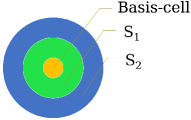
Figure 17: The sketch of $\mathbb{E}$

5.2.2 The order of T-structure-branches in $\mathbb{E}$

By Lemma 5.17, each T-connection is covered by a T-structure-branch. Assume that the T-connections in $\mathbb{E}$ are $\mathcal{TC}_{0},\mathcal{TC}_{1},...,\mathcal{TC}_{n}$, we denote $\mathcal{TSB}_{i}$ as the corresponding T-structure-branch of $\mathcal{TC}_{i},i=0,...,n$. For each $\mathcal{TSB}_{i}$, we give the Algorithm 2 to order the T-structures in $\mathcal{TSB}_{i},i=0,...,n$. And then, sort $\mathcal{TSB}_{i},i=0,...,n$ in descending level order.

Input: $\mathcal{TSB}:\{\mathcal{T}_{0},...,\mathcal{T}_{m}\}$

Output: The order sorted T-structure-branch

1Give an empty T-structure-branch $\mathcal{TSB}_{0}$;

2 $\mathcal{TSB}_{0}\leftarrow$ the T-structure (T-structures) with the lowest level in $\mathcal{TSB}$;

3 Remove each T-structure of $\mathcal{TSB}_{0}$ from $\mathcal{TSB}$;

4 while $|\mathcal{TSB}|>0$ do

5       for $i=0,i<|\mathcal{TSB}_{0}|,i++$ do

6             Give an empty T-structure vector $V$;

7             for $j=0;j<|\mathcal{TSB}|;j++$ do

8                   if $\mathcal{TSB}_{0}[i]$ is connected to $\mathcal{TSB}[j]$  then

9                         $V\leftarrow\mathcal{TSB}[j]$;

10                        

11                  

12            Remove each T-structure of $V$ from $\mathcal{TSB}$;

13             Sort T-structures of $V$ in descending level order;

14             $\mathcal{TSB}_{0}\leftarrow$ each T-structure of $V$;

15            

16      

17Output $\mathcal{TSB}_{0}$;

Algorithm 2 The algorithm to sort the T-structures for each T-structure-Branch

5.2.3 The B-ordinates of $p(x,y)$ on $\mathcal{TC}_{0}$

In this subsection, we use T-structures to calculate the B-ordinates of $p(x,y)$ on $\mathcal{TC}_{0}$. We denote the T-rectangle-domain of $\mathcal{TC}_{0}$ as $\mathcal{TRD}_{0}$. By Lemma 5.17, $\mathcal{TC}_{0}$ is covered by $\mathcal{TSB}_{0}$, $\mathcal{TSB}_{0}$ is the lowest level T-structure-branch in $\mathbb{E}$. $\mathcal{TC}_{0}$ is also the lowest level T-connection in $\mathbb{E}$. The B-ordinates on the T-cells that belong to $\mathcal{TC}_{0}$ can be calculated by T-structures in $\mathcal{TSB}_{0}:{\mathcal{T}_{0},...,\mathcal{T}_{m}}$. $\mathcal{T}_{0},...,\mathcal{T}_{m}$ are already sorted by Algorithm 2, and $\mathcal{T}_{0}$ is the T-structure with the lowest level.

As $\mathcal{TC}_{0}$ is also the lowest level T-connection in $\mathbb{E}$, we give the initialization as follows:

Initialization 1

As $\mathcal{TC}_{0}$ is also the lowest level T-connection in $\mathbb{E}$, we give the initialization as follows:

As $\mathcal{T}_{0}$ is the T-structure with the lowest level in $\mathcal{TSB}_{0}$, we give the lemma as follows:

Lemma 5.22

The two end-points of $\mathcal{T}_{0}$ are crossing-vertices.

Proof 12

We prove the lemma by reduction to absurdity. If one of the end-points is a T-junction, then a lower level T-structure $\mathcal{T}^{\prime}_{0}$, which connects to $\mathcal{T}_{0}$ at a T-junction, exists. Then, the level of $\mathcal{T}^{\prime}_{0}$ is lower than the level of $\mathcal{T}_{0}$ and $\mathcal{T}^{\prime}_{0}$ belongs to $\mathcal{TSB}_{0}$. It contradicts the order of the T-structures in $\mathcal{TSB}_{0}$. Thus, the two end-points of $\mathcal{T}_{0}$ are crossing-vertices. The lemma is proved.

(a) The denotes of $\mathcal{T}_{0}$	(a) $C_{0}$ is a T-cell	(b)$C_{0}$ is a P-cell

Figure 18: $\mathcal{T}_{0}$.

By Lemma 5.22, the two end-points of $\mathcal{T}_{0}$ are crossing-vertices. Without loss of generality, we use the vertical T-structure in Fig. 18(a) to illustrate $\mathcal{T}_{0}$. We denote the two end-points of $\mathcal{T}_{0}$ as $v_{1}$ and $v_{2}$ respectively, denote the mother-cell of $\mathcal{T}_{0}$ as $C_{1}$. $C_{1}$ is also the one-neighbor-cell of $\mathcal{TC}_{0}$. We can calculate the corresponding B-ordinates of $\mathcal{T}_{0}$ via the bilinear function associated with each end-point of $\mathcal{T}_{0}$. From Theorem 5.20, if the weights or B-ordinates on the adaptive nodes of the bilinear function on each end-point of $\mathcal{T}_{0}$ are given, we can use the bilinear function to calculate the corresponding B-ordinates for each end-point. We give the theorem to obtain the corresponding B-ordinates on $\mathcal{T}_{0}$ as follows:

(a)	(b)	(c)	(d)	(e)

Figure 19: Four adaptive nodes for a crossing-vertex of $\mathcal{T}_{0}$.

Theorem 5.23

For each end-point of $\mathcal{T}_{0}$, there exists a group of adaptive nodes that the weight or B-ordinate on each node is given, the corresponding B-ordinates of $p(x,y)$ on $\mathcal{T}_{0}$ can be calculated by Theorem 5.20.

Proof 13

Without loss of generality, we first discuss the adaptive nodes for $v_{1}$, the adaptive nodes for $v_{2}$ can be obtained similar to $v_{1}$. We denote the level of $C_{i}$ as $l(C_{i}),i=1,2,3$ for convenience. If $C_{i}$ is a T-cell, without loss of generality, we assume the $C_{i}$ belongs to $\mathcal{TC}_{i}$, the level of $\mathcal{TC}_{i}$ is denoted as $l(\mathcal{TC}_{i}),i=1,2,3$ for convenience. By Definition 5.16, the level of $\mathcal{TC}_{0}$ is $l(C_{1})$.

If $C_{1}$ is a T-cell, we use Fig 18(b) to illustrate the adaptive nodes. Assume that $C_{1}$ is a sub-cell of the T-structure $\mathcal{T}^{\prime}$. As $C_{1}$ is the mother-cell of $\mathcal{T}_{0}$, the level of $\mathcal{T}^{\prime}$ is lower than $l(C_{1})$. If $\mathcal{T}^{\prime}$ belongs to the T-structure-branch $\mathcal{TSB}^{\prime}$, the level of $\mathcal{TSB}^{\prime}$ is lower than $l(C_{1})$. We denote the T-connection corresponding to $\mathcal{TSB}^{\prime}$ as $\mathcal{TC}^{\prime}$, the level of $\mathcal{TC}^{\prime}$ is lower than $l(C_{1})$. By Initialization 1, the nine B-ordinates of $p(x,y)$ on each T-cell belongs to $\mathcal{TC}^{\prime}$ are $0$. The four B-ordinates on “$\bullet$” of $C_{0}$ in Fig 18(b) are given by the initialization, we can choose $P^{1}_{02}(s^{1}_{02},t^{1}_{02}),P^{1}_{12}(s^{1}_{12},t^{1}_{12}),P^{1}_{01}(s^{1}_{01},t^{1}_{01})$ and $P^{1}_{11}(s^{1}_{11},t^{1}_{11})$ as the adaptive nodes of $v_{1}$.

If $C_{1}$ is a P-cell, we use Fig. 18(c) to illustrate the two given adaptive nodes: the weights on “$\blacktriangle$” and “$\bullet$” are given by Equation (22). As $C_{1}$ is a P-cell, the weight on “$\bullet$” is also the B-ordinate on the centre domain point of $C_{0}$. By Proposition 5.21, the points on “$\blacktriangle$” and “$\bullet$” can be used as two of the four adaptive nodes. As $C_{1}$ is the one-neighbor-cell of $\mathcal{TC}_{0}$, “$\blacktriangle$” and “$\bullet$” are on the line that is parallel to $E_{1}$, which is shown as the green dashed line in Fig. 18(c).

In the next discussion, we need to obtain the whole group of adaptive nodes for $v_{1}$. We use Fig. 19 to illustrate the adaptive nodes, the notations are the same as that in Fig . 18(c). A careful analysis of the type of $C_{i}$ and $l(C_{i}),i=1,2,3$ will help us to obtain the four adaptive nodes. We have the following two situations by discuss the type of $C_{i},i=2,3$:

1. $C_{2}$ is a P-cell. If $C_{2}$ is a P-cell, the vertices of $C_{1}$ and $C_{2}$ on $E$ are the same, and it is a crossing-vertex, then $l(C_{2})=l(C_{1})$. As the B-ordinate of $p(x,y)$ on the centre domain-point of $C_{2}$ is given by Equation 22, the centre domain-point can be used as one node of the four adaptive nodes. And then, we discuss the type of $C_{3}$ to obtain the adaptive nodes.

2. $C_{2}$ is T-cell. If $C_{2}$ is a T-cell, we assume that $C_{2}$ belongs to the T-connection $\mathcal{TC}_{2}$. As $C_{1}$ is a P-cell that is adjacent to $\mathcal{TC}_{2}$, the level of the one-neighbor-cell of $\mathcal{TC}_{2}$ is less than or equal to $l(C_{1})$, we obtain that $l(\mathcal{TC}_{2})\leqslant l(C_{1})$. If $l(\mathcal{TC}_{2})=l(C_{1})$, $C_{1}$ is the one-neighbor-cell of $\mathcal{TC}_{2}$; otherwise, $C_{1}$ is not the one-neighbor-cell of $\mathcal{TC}_{2}$. And then, we discuss the type of $C_{3}$ to obtain the adaptive nodes.

Consider case 1. If $C_{2}$ is a P-cell, the B-ordinate of $p(x,y)$ on the centre domain-point of $C_{2}$ is given by Equation 22. We use Fig. 19(a) and (b) to discuss the adaptive nodes. We denote the domain-point of $C_{2}$ as $P^{2}_{11}(s^{2}_{11},t^{2}_{11})$ in Fig. 19(a) and (b). By Proposition 5.21, $P^{2}_{11}$ can be used as one of the four adaptive nodes. $P^{2}_{11}$ is on a line that is perpendicular to the green dashed line, the two lines construct a cross, which can be denoted as $X_{0}$. We discuss the whole group of adaptive nodes as follows:

1. $C_{3}$ is a p-cell. If $C_{3}$ is a P-cell, the B-ordinate of $p(x,y)$ on the centre domain-point of $C_{3}$ is given by Equation 22. We denote the domain-point of $C_{3}$ as $P^{3}_{11}(s^{3}_{11},t^{3}_{11})$ in Fig. 19(a). By Proposition 5.21, $P^{3}_{11}$ can be used as one of the four adaptive nodes. As $P^{3}_{11}$ is not on the cross $X_{0}$, we can choose the four nodes as $P^{1}_{11}(s^{1}_{11},t^{1}_{11})$, $P^{2}_{11}(s^{2}_{11},t^{2}_{11})$, $P^{3}_{11}(s^{3}_{11},t^{3}_{11})$ and $P^{0}(s^{0},t^{0})$ in Fig. 19(a).

2. $C_{3}$ is a T-cell. If $C_{3}$ is a T-cell, we assume $C_{3}$ as a T-cell belongs to the T-connection $\mathcal{TC}_{3}$, as $C_{2}$ is a P-cell adjacent to $\mathcal{TC}_{3}$, the level of the one-neighbor-cell of $\mathcal{TC}_{3}$ is not higher than $l(C_{2})$, we obtain that $l(\mathcal{TC}_{3})\leqslant l(C_{2})$.

   1. $l(\mathcal{TC}_{3})<l(C_{2})$. If $l(\mathcal{TC}_{3})<l(C_{2})$, as $l(C_{2})=l(C_{1})$, we obtain $l(\mathcal{TC}_{3})<l(C_{1})$. By Initialization 1, the nine B-ordinates of $p(x,y)$ on each T-cell of $\mathcal{TC}_{3}$ are given, the B-ordinate of $p(x,y)$ on the centre domain-point of $C_{3}$ is given. Similar to (1) in case 1, we can choose the four nodes as $P^{1}_{11}(s^{1}_{11},t^{1}_{11})$, $P^{2}_{11}(s^{2}_{11},t^{2}_{11})$, $P^{3}_{11}(s^{3}_{11},t^{3}_{11})$ and $P^{0}(s^{0},t^{0})$ in Fig. 19(a).

   2. $l(\mathcal{TC}_{3})=l(C_{2})$. If $l(\mathcal{TC}_{3})=l(C_{2})$, $C_{2}$ is the one-neighbor-cell of $\mathcal{TC}_{3}$. We denote the domain-centre of $\mathcal{TC}_{3}$ as $P^{3}(s^{3},t^{3})$ in Fig.19(b). As the weight on $P^{3}$ is given by Equation 22. By Proposition 5.21, $P^{3}$ can be used as one of the four adaptive nodes. As $P^{3}_{11}$ is not on the cross $X_{0}$, we can choose the four nodes as $P^{3}(s^{3},t^{3})$, $P^{1}_{11}(s^{1}_{11},t^{1}_{11})$, $P^{2}_{11}(s^{2}_{11},t^{2}_{11})$ and $P^{0}(s^{0},t^{0})$ in Fig. 19(b).

Consider case 2. If $C_{2}$ is a T-cell, $C_{2}$ is assumed as a cell belongs to $\mathcal{TC}_{2}$. As $l(\mathcal{TC}_{2})\leqslant l(C_{1})$, we discuss the adaptive nodes as follows:

1. $l(\mathcal{TC}_{2})=l(C_{1})$. If $l(\mathcal{TC}_{2})=l(C_{1})$, $C_{1}$ is the one-neighbor-cell of $\mathcal{TC}_{2}$. We use Fig. 19(c) and Fig. 19(d) to discuss the adaptive nodes. We denote the domain-centre of $\mathcal{TC}_{2}$ as $P^{2}(s^{2},t^{2})$ in Fig. 19(c) Fig. 19(d). The weight on the domain-centre is given by Equation 22. By Proposition 5.21, $P^{2}$ can be used as one of the four adaptive node, and $P^{2}$ is on a line that is perpendicular to the green dashed line, the two lines construct a cross, which can be denoted as $X_{1}$.

   1. $C_{3}$ is a P-cell. If $C_{3}$ is a P-cell, the B-ordinate on the centre domain-point of $C_{3}$ is given by Equation 22, we denote the centre domain-point of $C_{3}$ as $P^{3}_{11}(s^{3}_{11},t^{3}_{11})$ in Fig. 19(c). By Proposition 5.21, $P^{3}_{11}$ can be used as one of the four nodes. As $P^{3}_{11}$ is not on the cross $X_{1}$, we can choose the four nodes as $P^{3}_{11}(s^{3}_{11},t^{3}_{11})$, $P^{1}_{11}(s^{1}_{11},t^{1}_{11})$, $P^{2}(s^{2},t^{2})$ and $P^{0}(s^{0},t^{0})$ in Fig. 19(c).

   2. $C_{3}$ is a T-cell. If $C_{3}$ is a T-cell, we assume $C_{3}$ as a T-cell of the T-connection $\mathcal{TC}_{3}$. Then, $l(\mathcal{TC}_{3})$ is not equal to $l(C_{1})$. Otherwise, if $l(\mathcal{TC}_{3})=l(C_{1})$, as the one-neighbor-cell of $l(\mathcal{TC}_{3})$ is neither on $E_{2}$ nor on $E_{3}$. There exist some cross vertices of $\mathcal{TC}_{3}$ on $E_{2}$ or $E_{3}$, $\mathcal{TC}_{3}$ is split into several parts, it is contrary to the assumption. Thus, $l(\mathcal{TC}_{3})<l(C_{1})$ or $l(\mathcal{TC}_{3})>l(C_{1})$.

      1. $l(\mathcal{TC}_{3})<l(C_{1})$. If $l(\mathcal{TC}_{3})<l(C_{1})$, by Initialization 1, the nine B-ordinates of $p(x,y)$ on each T-cell in $\mathcal{TC}_{3}$ are given, the B-ordinate on the center domain-point of $C_{3}$ is given. Similar to (1)(a) in case 2, we can choose the four nodes as $P^{3}_{11}(s^{3}_{11},t^{3}_{11})$, $P^{1}_{11}(s^{1}_{11},t^{1}_{11})$, $P^{2}(s^{2},t^{2})$ and $P^{0}(s^{0},t^{0})$ in Fig. 19(c).

      2. $l(\mathcal{TC}_{3})>l(C_{1})$ If $l(\mathcal{TC}_{3})>l(C_{1})$, as $C_{3}$ is a cell divided by one cell of $\mathscr{T}^{k},k>=l_{1}$, $v_{3}$ is a crossing-vertex, and the one-neighbor-cell is either on $E_{2}$ or on $E_{3}$. As the weight on the domain-centre of $\mathcal{TC}_{3}$ is given by Equation 22, by Proposition 5.21, the domain-centre of $\mathcal{TC}_{3}$, which is denoted as $P^{3}(s^{3},t^{3})$ in Fig. 19(d), can be used as one of the four adaptive nodes. As $P^{3}$ is not on the cross $X_{1}$, we can choose the four nodes as $P^{3}(s^{3},t^{3})$, $P^{1}_{11}(s^{1}_{11},t^{1}_{11})$, $P^{2}(s^{2},t^{2})$ and $P^{0}(s^{0},t^{0})$ in Fig. 19(d).

2. $l(\mathcal{TC}_{2})<l(C_{1})$. If $l(\mathcal{TC}_{2})<l(C_{1})$. By Initialization 1, the B-ordinates of $p(x,y)$ on each T-cell of $\mathcal{TC}_{2}$ are given. By Proposition 5.21, the two domain-points, which are denoted as $P^{2}_{01}(s^{2}_{01},t^{2}_{01})$ and $P^{2}_{11}(s^{2}_{11},t^{2}_{11})$ in Fig.19(e), can be used as two of the four adaptive nodes. $P^{2}_{11}$ is on a line that is perpendicular to the green dashed line, the two lines construct a cross, which can be denoted as $X_{2}$. As $P^{2}_{01}$ is not on $X_{2}$, we can choose one group of adaptive nodes as $P^{2}_{01}(s^{2}_{01},t^{2}_{01})$, $P^{2}_{11}(s^{2}_{11},t^{2}_{11})$, $P^{0}(s^{0},t^{0})$ and $P^{1}_{11}(s^{1}_{11},t^{1}_{11})$ in Fig. 19(e).

From the discussion above, each group of nodes is adaptive. As the weight or B-ordinate on each node is given by the discussion, we can calculate the coefficients of the bilinear function on $v_{1}$. Similar to the situation of $v_{1}$, we can calculate the coefficients of the bilinear function on $v_{2}$. And then, using Theorem 5.20, we obtain the corresponding B-ordinates that satisfy the $C^{1}$ continuous condition on each edge of $\mathcal{T}_{0}$, we obtain the corresponding B-ordinates of $p(x,y)$ on $\mathcal{T}_{0}$. The theorem is proved.

(a) $v_{2}$ is a crossing-vertex	(b) $v_{2}$ is a T-junction

Figure 20: Other T-structures.

Corollary 5.24

The corresponding B-ordinates of $p(x,y)$ on $\mathcal{T}_{i},i=1,...,m$ can be calculated by Lemma 5.18.

Proof 14

We can obtain all of the corresponding B-ordinates of $\mathcal{T}_{0}$ via the Theorem 5.23. As the T-structures in $\mathcal{TSB}_{0}$ are sorted as $\mathcal{T}_{0},\mathcal{T}_{1},...\mathcal{T}_{m}$ via Algorithm 2, $\mathcal{T}_{1}$ is connected to $\mathcal{T}_{0}$. Without loss of generality, we assume that $\mathcal{T}_{1}$ is connected to $\mathcal{T}_{0}$ at $v_{2}$, which is shown in Fig. 20. $v_{2}$ is a crossing-vertex in Fig. 20 (a) or T-junction in Fig. 20 (b), the corresponding B-ordinates of $v_{2}$ are obtained. In Fig. 20, $C_{0}$ is denoted as the mother-cell of $\mathcal{T}_{1}$, and the B-ordinates on $P^{0}_{01}$ and $P^{0}_{11}$ are given. Replace $P^{0}$ in Fig. 18 with $P^{0}_{01}$ in Fig. 20, we can obtain at least one group adaptive nodes for $v_{1}$ in Fig. 20. The corresponding bilinear function for $v_{1}$ can be obtained naturally. And then, we can calculate the corresponding B-ordinates of $\mathcal{T}_{1}$ via Lemma 5.18. By Algorithm 2, $\mathcal{T}_{i}$ is connected to one of $\mathcal{T}_{0},...,\mathcal{T}_{i-1},i=1,...,m.$ In a similar way to $\mathcal{T}_{1}$, we can obtain the corresponding B-ordinates of $p(x,y)$ on $\mathcal{T}_{i},i=2,...,m.$ The corollary is proved.

We give algorithm 3 to illustrate the process for calculating the corresponding B-ordinates on each T-structure in $\mathcal{TSB}_{0}$.

Input: $\mathcal{TSB}_{0}:\{\mathcal{T}_{0},...,\mathcal{T}_{m}\}$

Output: The B-ordinates of each T-cell in $\mathcal{TC}_{0}$

1Calculate the corresponding B-ordinates of $\mathcal{TSB}_{0}[0]$;

2 $V\leftarrow\mathcal{TSB}_{0}[0]$;

3 Remove $\mathcal{TSB}_{0}[0]$ from $\mathcal{TSB}_{0}$;

4 while $|\mathcal{TSB}_{0}|>0$ do

5       for $i=1,i<|\mathcal{TSB}_{0}|,i++$ do

6             Bool Connected=false;

7             for $j=0;j<|V|;j++$ do

8                   if $\mathcal{TSB}_{0}[i]$ is connected to $V[j]$ at one end point of $\mathcal{TSB}_{0}[i]$  then

9                         Connected=true;

10                  

11            if Connected then

12                  Calculate the corresponding B-ordinates on the other end-point of $\mathcal{TSB}_{0}[i]$;

13                   Using Lemma 5.18 to calculate the corresponding B-ordinates on $\mathcal{TSB}_{0}[i]$;

14                   Remove $\mathcal{TSB}_{0}[i]$ from $\mathcal{TSB}_{0}$;

15                   $V\leftarrow\mathcal{TSB}_{0}[i]$;

16            

17      

18Using the $C^{1}$ continuous conditions on the rest edges that the B-ordinates are not obtained;

Algorithm 3 Calculate the B-ordinates for each T-cell in $\mathcal{TC}_{0}$

Theorem 5.25

The B-ordinates of $p(x,y)$ on each T-cell belongs to $\mathcal{TC}_{0}$ can be calculated by Algorithm 3.

Proof 15

By Lemma 5.17, the T-cells in $\mathcal{TC}_{0}$ are covered by $\mathcal{TSB}_{0}$, The B-ordinate on the centre domain-point of each T-cell in $\mathcal{TC}_{0}$ is obtained. As the corresponding B-ordinates on each T-structure in $\mathcal{TSB}_{0}$ are calculated, we can calculate the rest B-ordinates on each T-cell of $\mathcal{TC}_{0}$ via $C^{1}$ continuous conditions. The theorem is proved.

5.2.4 The B-ordinates of $p(x,y)$ on $\mathcal{TC}_{i},i=1,...,n$

The B-ordinates on the T-cells of $\mathcal{TC}_{0}$ are calculated in Section 5.2.3. The B-ordinates on the T-cells of the rest T-connections $\mathcal{TC}_{i},i=1,...,n$ can be calculated similarly.

Theorem 5.26

For each T-connection in $\mathbb{E}$, we can obtain the B-ordinates of $p(x,y)$ on the T-cells belong to the T-connection.

Proof 16

As $\mathcal{TC}_{i},i=0,...,n$ are in the same descending level order as $\mathcal{TSB}_{i},i=0,...,n$. We can calculate all of the B-ordinates on $\mathcal{TC}_{0}$ via algorithm 3. And then, $\mathcal{TC}_{1}$ is the T-connection whose level is the lowest. We can calculate B-ordinates on $\mathcal{TC}_{1}$ in the same way as $\mathcal{TC}_{0}$. By this analogy, we can calculate the B-ordinates on each T-connection $\mathcal{TC}_{i},i=2,...,n$ by Algorithm 3. The theorem is proved.

Till now, we can calculate the B-ordinates of $p(x,y)$ on the the T-cells belong to $\mathcal{TC}_{i},i=0,...,n$. And we give the following theorem to obtain the B-ordinates of $p(x,y)$:

Theorem 5.27

For the polynomial function $p(x,y)\in\overline{\mathbf{S}}^{2}(\mathscr{T})$, the weights are denoted by Equation (22), $\mathbb{E}$ denotes the domain that covers $sup(p(x,y))$. Then, the B-ordinates on each cell in $\mathbb{E}$ can be calculated by Theorem 5.26 and $C^{1}$ continuous conditions.

Proof 17

As the B-ordinate on the center domain-point of each T-cell in $\mathbb{E}$ is calculated by theorem 5.26, and the B-ordinate on the center domain-point of each P-cell in $\mathbb{E}$ is given by Equation(22). The B-ordinates on each cell in $\mathbb{E}$ can be calculated via $C^{1}$ continuous conditions. The theorem is proved.

For each cell $C\in\mathbb{E}$, if at least one B-ordinate of $C$ is nonzero, we save $C$ to the support of $p(x,y)$. We can use Bernstein-B$\acute{e}$zier to express $p(x,y)$, which is $C^{1}$ continuous on the support. Then, we obtained a polynomial function with local support of $\overline{\mathbf{S}}^{2}(\mathscr{T})$.

5.3 Simplify the hierarchical T-mesh

In particular, if the T-l-edge $E$ only contains $V_{0}$ vertices, $\dim W[E]=(V_{0}-d-1)_{+}:=\max(0,V_{0}-d-1)$ holds for $\mathbf{S}^{d}(\mathscr{T})$, $E$ is defined as a trivial l-edge[24, 27] if $(V_{0}-d-1)_{+}=0$ . For the T-l-edge $E$ with one interior crossing-vertex, we say $E$ is a trivial l-edge. As $\dim W[E]=0$, we can remove $E$ from $\mathscr{T}$, and the polynomial functions of the spline spaces will not change.

Fig. 21 shows the simplification of a hierarchical T-mesh. As the green lines are trivial l-edges in $\mathscr{T}_{0}$, remove them, we obtain $\mathscr{T}_{1}$. As the blue line is a trivial l-edges in $\mathscr{T}_{1}$, remove it, we obtain $\mathscr{T}_{2}$. $\mathscr{T}_{2}$ is denoted as the simplification of $\mathscr{T}_{0}$.

(a) $\mathscr{T}_{0}$	(b) $\mathscr{T}_{1}$	(c) $\mathscr{T}_{2}$

Figure 21: Simplification of a T-mesh.

It is natural that we can remove meshlines that do not contribute to the dimension of the spline space [14]. The simplification can reduce the number of T-structures, decrease the amount of calculation, and remove some overhanging edges from CVR graph. We give Algorithm 4 to construct a biquadratic polynomial function $p(x,y)\in\overline{\mathbf{S}}^{2}(\mathscr{T})$, where $\mathscr{T}$ is the simplified T-mesh.

Input: $q(x,y)\in\overline{\mathbf{S}}^{0}(\mathscr{G})$

Output: The B-ordinates of $p(x,y)\in\overline{\mathbf{S}}^{2}(\mathscr{T})$

1Give the weights on each domain of $\mathscr{T}$ by Equation 22 ;

2 Obtain $\mathbb{E}:\{\mathcal{TC}_{0},...,\mathcal{TC}_{n}\}\cup\{\mathcal{PC}_{0},...,\mathcal{PC}_{l}\}$;

3 Obtain each T-structure-branch $\mathcal{TSB}_{i}$ corresponding to $\mathcal{TC}_{i},i=0,...,n$;

4 Sort the T-structures in $\mathcal{TSB}_{i}$ via algorithm 2, $i=0,...,n$;

5 Sort $\mathcal{TSB}_{i},i=0,...,n$ in descending level order;

6 Calculate the corresponding B-ordinates of $p(x,y)$ on $\mathcal{TSB}_{i}$ via Algorithm 3;

7 Calculate the B-ordinates on the cells in $\mathbb{E}$ via $C^{1}$ continuous conditions;

8 Save the support of $p(x,y)$ on $\mathscr{T}$;

Algorithm 4 Calculate the B-ordinates for $p(x,y)$

By Algorithm 4, we obtain the basis function of $\overline{\mathbf{S}}^{2}(\mathscr{T})$ corresponding to the basis function of $\overline{\mathbf{S}}^{0}(\mathscr{G})$, and we give the theorem as:

Theorem 5.28

Each basis function of $\overline{\mathbf{S}}^{0}(\mathscr{G})$ corresponds to a biquadratic polynomial function of $\overline{\mathbf{S}}^{2}(\mathscr{T})$.

Proof 18

Given the basis function $q(x,y)\in\overline{\mathbf{S}}^{0}(\mathscr{G})$, denote the domain weights for $p(x,y)\in\overline{\mathbf{S}}^{2}(\mathscr{T})$ by Equation (22), we can calculate the B-ordinates for $p(x,y)$ by algorithm 4. The theorem is proved.

So far, we construct the biquadratic polynomial function of $\overline{\mathbf{S}}^{2}(\mathscr{T})$ via a piecewise constant basis function of $\overline{\mathbf{S}}^{0}(\mathscr{G})$.

6 The isomorphic bivariate spaces and properties

In this section, we discuss the bijective property of the mapping that constructed in Section 4. Some properties of the basis functions we constructed in Section 5 are also discussed.

6.1 The bijective property of the mapping

First, by Section 4 and Section 5, we give a theorem about the mapping as follows:

Theorem 6.29

For the hierarchical T-mesh $\mathscr{T}$, $\mathscr{G}$ denotes the CVR graph of $\mathscr{T}$. The mapping between $\overline{\mathbf{S}}^{2}(\mathscr{T})$ and $\overline{\mathbf{S}}^{0}(\mathscr{G})$ is bijective, and $\overline{\mathbf{S}}^{2}(\mathscr{T})$ is isomorphic to $\overline{\mathbf{S}}^{0}(\mathscr{G})$.

Proof 19

By Theorem 4.14, the mapping from $\overline{\mathbf{S}}^{2}(\mathscr{T})$ to $\overline{\mathbf{S}}^{0}(\mathscr{G})$ is an injective mapping. By Theorem 5.28, each basis function of $\overline{\mathbf{S}}^{0}(\mathscr{G})$ corresponds to a polynomial function of $\overline{\mathbf{S}}^{2}(\mathscr{T})$, the mapping is surjective. Thus, the mapping is bijective, and $\overline{\mathbf{S}}^{2}(\mathscr{T})$ is isomorphic to $\overline{\mathbf{S}}^{0}(\mathscr{G})$.

As the properties of the piecewise constant basis functions over the CVR graph are simple and clear, we use them to discuss the properties of the basis function belongs to biquadratic spline space over the hierarchical T-mesh as follows:

6.2 Properties

In this subsection, we denote the extension of $\mathscr{T}$ as $\mathscr{T}^{\varepsilon}$, and we denote the CVR graph of $\mathscr{T}^{\varepsilon}$ as $\mathscr{G}^{\varepsilon}$. We discuss the properties of basis functions of $\mathbf{S}^{2}(\mathscr{T})$ as follows:

Theorem 6.30

The basis functions of $\mathbf{S}^{2}(\mathscr{T})$ hold the properties of linearly independence, completeness.

Proof 20

Apply the mapping to $\overline{\mathbf{S}}^{2}(\mathscr{T}^{\varepsilon})$ and $\overline{\mathbf{S}}^{2}(\mathscr{G}^{\varepsilon})$. By Theorem 6.29, the mapping between $\overline{\mathbf{S}}^{2}(\mathscr{T}^{\varepsilon})$ and $\overline{\mathbf{S}}^{2}(\mathscr{G}^{\varepsilon})$ is bijective, and $\overline{\mathbf{S}}^{2}(\mathscr{T}^{\varepsilon})$ is isomorphic to $\overline{\mathbf{S}}^{0}(\mathscr{G}^{\varepsilon})$. As the basis functions of $\overline{\mathbf{S}}^{0}(\mathscr{G}^{\varepsilon})$ are linearly independent and complete, the basis functions of $\overline{\mathbf{S}}^{2}(\mathscr{T}^{\varepsilon})$ are also linearly independent and complete. By Theorem 2.2, and the basis functions of $\mathbf{S}^{2}(\mathscr{T})$ are linearly independent and complete on $\mathscr{T}$.

Theorem 6.31

All the basis functions of $\mathbf{S}^{2}(\mathscr{T})$ have the property of unit partition.

Proof 21

Assume that the basis functions of $\overline{\mathbf{S}}^{2}(\mathscr{T}^{\varepsilon})$ are $p_{i}(x,y)$, the basis functions of $\overline{\mathbf{S}}^{0}(\mathscr{G}^{\varepsilon})$ are $q_{i}(x,y)$, and $\mathbf{\Phi}^{-1}(q_{i})=p_{i}$ where $i=1,2,...,N_{\mathscr{G}^{\varepsilon}}$. As the space is a linear space, we obtain

$$\sum^{N_{\mathscr{G}^{\varepsilon}}}_{i=1}p_{i}=\sum^{N_{\mathscr{G}^{\varepsilon}}}_{i=1}\mathbf{\Phi}^{-1}(q_{i})=\mathbf{\Phi}^{-1}(\sum^{N_{\mathscr{G}^{\varepsilon}}}_{i=1}(q_{i})).$$

As $\sum^{N_{\mathscr{G}^{\varepsilon}}}_{i=1}(q_{i})=1$ is true for each g-cell of $\mathscr{G}^{\varepsilon}$, the weight on each interior domain of $\mathscr{T}^{\varepsilon}$ is $1$. By Algorithm 4, the B-ordinates on each cell of $\mathscr{T}$ are $1$.

Thus, $\sum^{N_{\mathscr{G}^{\varepsilon}}}_{i=1}p_{i}=1$ is true on $\mathscr{T}$, by Theorem 2.2, the theorem is proved.

Thus, the mapping is an isomorphism and the basis functions that we construct for $\mathbf{S}^{2}(\mathscr{T})$ hold the properties of linearly independence, completeness and partition of unity.

7 Surface fitting

Given an open surface triangulation with vertices $V_{i},i=0,..,N$ in 3D space, the corresponding parameter values $(x_{i},y_{i}),i=0,..,N$ are obtained by the parametrization in [32], we denote the triangle on the triangulation mesh as $\Delta$. the parameter mesh is a triangle mesh and the parameter domain is $[0,1]\times[0,1]$.

To construct a spline to fit the given surface, we need to compute all the basis functions $b_{j}(x,y),j=1,...,m$ and their corresponding control points $P_{j},j=1,...,m$. We denote the fitting spline $S(x,y)={\sum}^{m}_{j=1}P_{j}b_{j}(x,y)$. To find the control points, we just need to solve an linear system

$$S(x_{k},y_{k})={V^{\prime}}_{k},k=1,2,...,m,$$

where $(x_{k},y_{k})=(\frac{x_{i_{k}}+x_{i_{k}+1}}{2},\frac{y_{i_{k}}+y_{i_{k}+1}}{2})$ is the domain-centre of the domain $[x_{i_{k}},x_{i_{k}+1}]\times[y_{i_{k}},y_{i_{k}+1}]$. $(x_{k},y_{k})\in\Delta_{l}:((x_{k_{1}},y_{k_{1}}),(x_{k_{2}},y_{k_{2}}),(x_{k_{3}},y_{k_{3}}))$, $(x_{k},y_{k})=w_{k_{1}}(x_{k_{1}},y_{k_{1}})+w_{k_{2}}(x_{k_{2}},y_{k_{2}})+w_{k_{3}}(x_{k_{3}},y_{k_{3}})$, and ${V^{\prime}}_{k}=w_{k_{1}}V_{k_{1}}+w_{k_{2}}V_{k_{2}}+w_{k_{3}}V_{k_{3}}$.

The surface fitting scheme repeats the following two steps until the fitting error in each cell is less than the given tolerance $\varepsilon$.

1. Compute all the control points for all the basis functions.

2. Find all the cells whose errors are greater than the given error tolerance $\varepsilon$, then subdivide these cells into four subcells to form a new mesh, simplify the new mesh, and construct basis functions for the new mesh. The fitting error on cell $C$ is $max_{(x,y)\in C}=\parallel V(x,y)-S(x,y)\parallel$.

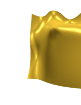
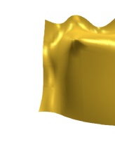
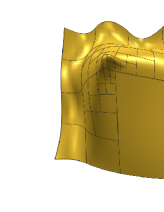
(a) An open surface patch

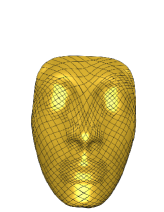
(b) Nefertiti face

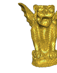
(c) Gargoyle

(d) Female head

Figure 22: Original meshes (left), result surfaces (middle), surfaces with T-meshes (right)

Four examples are provided to illustrate the above surface fitting scheme in Fig. 22. The iteration number (n), the dimensions of the spline spaces, the max error and the CPU time on 64 bit operating system are shown in Table 3.

model		n		dim		max error		t(s)
A surface patch		4		33		2.4 $\times 10^{-5}$		0.293
Nefertiti face		4		913		2.2 $\times 10^{-3}$		5.67
Gargoyle		11		4908		7.8 $\times 10^{-3}$		101.25
Female head		13		4256		6.0 $\times 10^{-3}$		150.38

Table 3: Experiment data.

8 Conclusions and future works

We give bijective mapping between the biquadratic spline space over a hierarchical T-mesh and the piecewise constant spline space over the corresponding CVR graph. And we obtain the conclusion that the biquadratic spline space is isomorphic to the piecewise constant spline space. By the bijective mapping, we proposed a novel method to discuss the dimensions of the biquadratic spline spaces over hierarchical T-meshes. We construct the basis functions of the biquadratic spline spaces via a novel structure, which is called a T-structure. Our method is general when the level difference of the hierarchical T-meshes is more than one. We overcome the limitations in [28], and we need not subdivide the extra cells to maintain the level different is less or equal to $1$. To reduce the computation, we give the simplifications of the hierarchical T-meshes. Our method is easy operative, and some numerical experiments are given to show our method is effective. By the bijective mapping, it is easy to prove that the basis functions hold the properties of linearly independence, completeness and partition of unity.

As the mapping we construct is an isomorphism, we will apply our basis functions to IGA and models with high genus in the future. This mapping provides a new idea for us to study high-order spline spaces with low-order spline spaces. We are also working to extend our work to high order spline spaces. The 3-variate case is also a considerable question. As some edges do not contribute to our dimension, improving our subdivision rules is also a considerable idea. We will also consider improving our basis construction method to reduce the computational overload in the future.

References

References

- [1] David R Forsey and Richard H Bartels. Hierarchical B-spline refinement. ACM Siggraph Computer Graphics, 22(4):205–212, 1988.
- [2] A-V Vuong, Carlotta Giannelli, Bert Jüttler, and Bernd Simeon. A hierarchical approach to adaptive local refinement in isogeometric analysis. Computer Methods in Applied Mechanics and Engineering, 200(49-52):3554–3567, 2011.
- [3] Carlotta Giannelli, Bert Jüttler, and Hendrik Speleers. THB-splines: The truncated basis for hierarchical splines. Computer Aided Geometric Design, 29(7):485–498, 2012.
- [4] Dominik Mokriš, Bert Jüttler, Carlotta Giannelli. On the completeness of hierarchical tensor-product B-splines. Journal of Computational and Applied Mathematics, 271:53–70, 2014.
- [5] Dominik Mokriš, Bert Jüttler. TDHB-splines: the truncated decoupled basis of hierarchical tensor-product splines. Computer Aided Geometric Design, 31(7-8):531–544, 2014.
- [6] Thomas W Sederberg, Jianmin Zheng, Almaz Bakenov, and Ahmad Nasri. T-splines and T-NURCCs. ACM Transactions on Graphics, 22(3):477–484, 2003.
- [7] Thomas W Sederberg, David L Cardon, G Thomas Finnigan, Nicholas S North, Jianmin Zheng, and Tom Lyche. T-spline simplification and local refinement. ACM Transactions on Graphics, 23(3):276–283, 2004.
- [8] A. Buffa, D.cho, G.Sangalli. Linear independence of the T-spline blending functions associated with some particular T-meshes. Computer Methods in Applied Mechanics and Engineering, 199(23-24):1437–1445, 2010.
- [9] Xin Li, Jianmin Zheng, Thomas W Sederberg, Thomas JR Hughes, Michael A Scott. On linear independence of T-spline blending functions. Computer Aided Geometric Design, 29(1):63–76, 2012.
- [10] Jiansong Deng, Falai Chen, Xin Li, Changqi Hu, Weihua Tong, Zhouwang Yang, Yuyu Feng. Polynomial splines over hierarchical T-meshes. Graphical Models, 70(4):76–86, 2008.
- [11] Nhon Nguyen Thanh, Kun Zhou. Extended isogeometric analysis based on PHT-splines for crack propagation near inclusions. International Journal for Numerical Methods in Engineering, 112(12):1777-1800, 2017.
- [12] Nhon Nguyen Thanh, Weidong Li, Jiazhao Huang, Kun Zhou. An adaptive isogeometric analysis meshfree collocation method for elasticity and frictional contact problems. International Journal for Numerical Methods in Engineering, 120(2):209-230, 2019.
- [13] Nhon Nguyen Thanh, Weidong Li, Kun Zhou. Static and free-vibration analyses of cracks in thin-shell structures based on an isogeometric-meshfree coupling approach. Computational Mechanics, 62(6):1287-1309, 2018.
- [14] Tor Dokken, Tom Lyche, Kjell Fredrik Pettersen. Polynomial splines over locally refined box-partitions. Computer Aided Geometric Design, 30(3):331–356, 2013.
- [15] Andrea Bressan. Some properties of LR-splines. Computer Aided Geometric Design, 30:778–794, 2013.
- [16] Francesco Patrizi, Tor Dokken. Linear dependence of bivariate Minimal Support and Locally Refined B-splines over LR-meshes. Computer Aided Geometric Design, 77, 2020.
- [17] Jiansong Deng, Falai Chen, Yuyu Feng. Dimensions of spline spaces over T-meshes. Journal of Computational and Applied Mathematics, 194(2):267–283, 2006.
- [18] Xin Li, Falai Chen. On the instability in the dimension of spline space over particular T-meshes. Computer Aided Geometric Design, 28(7):420–426, 2011.
- [19] Dmitry Berdinsky, Min-jae Oh, Tae-wan Kim, Bernard Mourrain. On the problem of instability in the dimension of a spline space over a T-mesh. Computers Graphics, 36(5):507–513, 2012.
- [20] Mourrain Bernard. On the dimension of spline spaces on planar T-meshes. Mathematics of Computation, 83(286):847–871, 2014.
- [21] Xin Li, Jiansong Deng. On the dimension of splines spaces over T-meshes with smoothing cofactor-conformality method. Computer Aided Geometric Design, 41:76–86, 2016.
- [22] Carlotta Giannelli, Bert Jüttler. Bases and dimensions of bivariate hierarchical tensor-product splines. Journal of Computational and Applied Mathematics, 239:162–178, 2013.
- [23] Jiansong Deng, Falai Chen, Liangbing Jin. Dimensions of biquadratic spline spaces over T-meshes. Journal of Computational and Applied Mathematics, 238:68–94, 2013.
- [24] Meng Wu, Jiansong Deng, Falai Chen. Dimension of spline spaces with highest order smoothness over hierarchical T-meshes. Computer Aided Geometric Design, 30(1):20–34, 2013.
- [25] Deepesh Toshniwala, Bernard Mourrain, Thomas J. R. Hughes. Polynomial spline spaces of non-uniform bi-degree on T-meshes: combinatorial bounds on the dimension. arXiv preprint arXiv:1903.05949, 2019.
- [26] Deepesh Toshniwala, Nelly Villamizar. Dimension of polynomial splines of mixed smoothness on T-meshes. Computer Aided Geometric Design, 80:101880, 2020.
- [27] Chao Zeng, Fang Deng, Xin Li, Jiansong Deng. Dimensions of biquadratic and bicubic spline spaces over hierarchical T-meshes. Journal of Computational and Applied Mathematics, 287:162–178, 2015.
- [28] Fang Deng, Chao Zeng, Meng Wu, Jiansong Deng. Bases of Biquadratic Polynomial Spline Spaces over Hierarchical T-meshes. Journal of Computational Mathematics, 35(1):91–120, 2017.
- [29] Chao Zeng, Fang Deng, Jiansong Deng. Bicubic hierarchical B-splines: Dimensions, completeness, and bases. Computer Aided Geometric Design, 38:1–23, 2015.
- [30] Larry L Schumaker, Lujun Wang. Approximation power of polynomial splines on T-meshes. Computer Aided Geometric Design, 29(8):599–612, 2012.
- [31] Chao Zeng, Meng Wu, Fang Deng, Jiansong Deng. Dimensions of spline spaces over non-rectangular T-meshes. Advances in Computational Mathematics, 42(6):1259–1286, 2016.
- [32] Floater M S. Parameterization and smooth approximation of surface triangulations. Computer Aided Geometric Design, 14(3):231–250, 1997.
- [33] Yuyu Feng, Falai Zeng, Jiansong Deng. Spline functions and approximaition theory. USTC Press, 2013.