Color charge correlations in the proton at NLO: beyond geometry based intuition

Abstract

Color charge correlators provide fundamental information about the proton structure. In this Letter, we evaluate numerically two-point color charge correlations in a proton on the light cone including the next-to-leading order corrections due to emission or exchange of a perturbative gluon. The non-perturbative valence quark structure of the proton is modelled in a way consistent with high-$x$ proton structure data. Our results show that the correlator exhibits startlingly non-trivial behavior at large momentum transfer or central impact parameters, and that the color charge correlation depends not only on the impact parameter but also on the relative transverse momentum of the two gluon probes and their relative angle. Furthermore, from the two-point color charge correlator, we compute the dipole scattering amplitude. Its azimuthal dependence differs significantly from a impact parameter dependent McLerran-Venugopalan model based on geometry. Our results also provide initial conditions for Balitsky-Kovchegov evolution of the dipole scattering amplitude. These initial conditions depend not only on the impact parameter and dipole size vectors, but also on their relative angle and on the light-cone momentum fraction $x$ in the target.

I Introduction

Revealing the proton and nuclear structure at high energies, or equivalently at small momentum fraction $x$, is one of the major tasks of the planned future nuclear deep inelastic scattering (DIS) facilities such as the Electron-Ion Collider (EIC) Boer:2011fh ; Accardi:2012qut ; Aschenauer:2017jsk ; AbdulKhalek:2021gbh in the US, LHeC/FCC-he Agostini:2020fmq at CERN and EicC in China Anderle:2021wcy . Thanks to the high energies and luminosities available at these future facilities, it will be possible to perform multi dimensional “proton imaging” and accurately determine the hadron structure not only as a function of momentum fraction $x$, but also including the geometric profile and intrinsic transverse momenta.

The color charge correlators provide fundamental information about the proton, and these correlators can be measured through various exclusive and inclusive processes at the EIC. For example, at leading order the light-cone gauge correlator is related to the average quark transverse momentum vector and to the Sivers asymmetry Burkardt:2003yg . Furthermore, in the mixed transverse momentum – transverse coordinate space representation, the color charge correlator can be related to the Wigner distribution Lorce:2011kd ; Belitsky:2003nz ; Ji:2003ak , which is the most fundamental object describing the proton structure, and to various other generalized parton distribution functions. This detailed information about the partonic structure of the proton can be accessed experimentally e.g. in dijet production or in vector meson – lepton azimuthal correlations in DIS, as recently argued in Refs. Hatta:2016dxp ; Hatta:2017cte ; Mantysaari:2020lhf ; Mantysaari:2019csc .

The first goal of this Letter is to present novel numerical results for the two-point color charge correlator in the proton at moderately small longitudinal momentum fraction $x$. Our numerical implementation is based on the recent computation presented in Ref. Dumitru:2020gla , where the two-point color charge correlator was computed within the framework of light-cone perturbation theory including the next-to-leading order (NLO) corrections due to emission or exchange of a perturbative gluon.

Our results show non-trivial features in the proton color field at moderate $x$. For example, one may naively assume the impact parameter dependence of these color charge correlations to follow the proton geometry, i.e. to be proportional to the transverse shape function of the proton. We, however, find that this geometric picture may only apply at large impact parameters; while the nature of color charge correlations near the center of the proton is much more intricate. In particular, our results show that the color charge correlation function depends not only on the impact parameter, but also on the relative transverse momentum of the two gluon probes and on the angle made by these two vectors. This is in contrast to the frequently used, intuitive, McLerran-Venugopalan (MV) model McLerran:1993ni ; McLerran:1993ka . Also, for some kinematic configurations, the correlator may in fact display negative (”repulsive”) correlations. The need for non-trivial correlations among “hot spots” in models for proton-proton scattering at high energies has been pointed out previously Albacete:2016pmp ; Albacete:2016gxu ; Albacete:2017ajt .

Our second goal here is to study the evolution of the dipole-proton scattering amplitude at moderately small $x$ values (say $x\sim 0.1,\ldots,0.01$), and to present initial conditions for high-energy quantum chromodynamics (QCD) evolution to yet smaller $x$. At high energies, where one is sensitive to the target structure at small $x$, the parton densities are so large Abramowicz:2015mha that individual quarks and gluons are not convenient degrees of freedom anymore. Instead, one considers eikonal interactions of the projectile with the effectively quasi-classical color field generated by the large $x$ partons in the target.

To describe QCD in this regime of high parton densities, an effective theory of QCD, the Color Glass Condensate (CGC) has been developed Iancu:2003xm ; Kovner:2005pe ; Gelis:2010nm ; Blaizot:2016qgz . In this approach, perturbative evolution equations such as the Balitsky-Kovchegov (BK) equation Kovchegov:1999yj ; Balitsky:1995ub describe the energy (or $x$) evolution of scattering amplitudes. The initial condition for this evolution encodes non-perturbative information about the proton structure, and has been previously determined by fitting the HERA structure function data Albacete:2010sy ; Lappi:2013zma ; Beuf:2020dxl .

In fact, the BK equation in its standard formulation evolves the wave function of the projectile, and the evolution “time” is given by the rapidity of the projectile Beuf:2014uia ; Ducloue:2019ezk ; Boussarie:2020fpb . Ducloué et al. have reformulated Ducloue:2019ezk BK evolution at NLO in terms of the target rapidity, which is the rapidity related to $x$. The resulting evolution equation is non-local in rapidity, which underscores the importance of $x$-dependent “initial conditions” for the dipole scattering amplitude as computed here. We emphasize that such an initial condition is a necessary ingredient for all phenomenological applications of the CGC framework; these applications are currently reaching NLO accuracy Lappi:2020ufv ; Beuf:2020dxl ; Ducloue:2017ftk ; Lappi:2015fma ; Lappi:2016fmu ; Hanninen:2017ddy ; Lappi:2016oup ; Boussarie:2016bkq ; Escobedo:2019bxn ; Beuf:2016wdz ; Altinoluk:2011qy ; Altinoluk:2014eka ; Roy:2019hwr , and this calls for a rigorous NLO level calculation of the initial condition. We also note that the calculation of the color charge correlator at NLO accuracy is required in order to determine the dependence on $x$, which enters as a cutoff on the gluon longitudinal momentum fraction, as discussed below.

II Color charge correlator

The central object of consideration in this paper is the two-point color charge correlator

$$\langle\rho^{a}(\vec{q}_{1})\,\rho^{b}(\vec{q}_{2})\rangle\equiv\delta^{ab}\,g^{2}G_{2}(\vec{q}_{1},\vec{q}_{2}),$$ (1)

where $g=\sqrt{4\pi\alpha_{\mathrm{s}}}$ is the strong coupling constant and $a,b$ are the external gluon colors. The notation $\langle\cdots\rangle$ denotes an expectation value between proton states, $\langle K|$ and $|P\rangle$, stripped of the delta-functions for conservation of transverse and light-cone momentum

$$\langle K|\,\rho^{a}(\vec{q}_{1})\,\rho^{b}(\vec{q}_{2})\,|P\rangle=16\pi^{3}\,P^{+}\\ \times\delta(P^{+}-K^{+})\,\delta(\vec{P}-\vec{K}-\vec{q}_{1}-\vec{q}_{2})\,\langle\rho^{a}(\vec{q}_{1})\,\rho^{b}(\vec{q}_{2})\rangle.$$ (2)

Furthermore, $\rho^{a}(\vec{q})=\rho^{a}_{\mathrm{qu}}(\vec{q})+\rho^{a}_{\mathrm{gl}}(\vec{q})$ denotes the operator which sums up the color charge densities of quarks (qu) and gluons (gl) with $q^{+}>0$; explicit expressions in terms of quark and gluon creation and annihilation operators are given in Ref. Dumitru:2020gla .

The insertion of the charge operators $\rho^{a}(\vec{q}_{1}),\rho^{b}(\vec{q}_{2})$ between the incoming and scattered proton states corresponds to the attachment of two static gluon probes (with amputated propagators) to the color charges in the proton, in all possible ways. The complete set of diagrams for $G_{2}$ at NLO and their explicit expressions are given in Ref. Dumitru:2020gla . The two static gluons that probe the proton structure carry transverse momenta $\vec{q}_{1}$ and $\vec{q}_{2}$, and the total momentum transfer to the proton reads

$$\vec{P}-\vec{K}=\vec{q}_{1}+\vec{q}_{2}.$$ (3)

In subsequent expressions, such as Eq. (4), we choose $\vec{P}=0$ for the incoming proton.

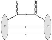
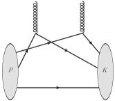
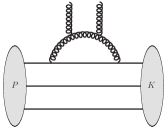
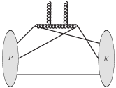
Figure 1: Examples for handbag (left) and cat’s ears (right) diagrams at LO (top) and at NLO (bottom).

Figure 1 shows examples for “handbag” and “cat’s ears” diagrams at leading order (LO) $g^{2}$ and at NLO $g^{4}$ in the strong coupling constant. The former are represented at LO by one-body operators so that the entire momentum transfer $\vec{K}$ to the proton flows into a single valence quark line. Therefore, for $\vec{q}_{1}\to-\vec{q}_{2}$ (i.e. $\vec{K}\to 0$) the LO handbag diagrams approach the normalization integral in Eq. (10), such that there is maximal wave function overlap. At leading order, the handbag diagram is proportional to the electromagnetic form factor, i.e. to the distribution $\langle\rho(\vec{q})\rangle$ of electric charge in the proton.

For large momentum transfer, on the other hand, wave function overlap in the handbag diagram is highly suppressed. At large $\vec{K}^{2}$, the wave function overlap is much greater for the cat’s ears diagram because the momentum transfer is shared by two (or even three, at NLO) valence quarks. Since $\vec{K}$ is the Fourier conjugate to the two-dimensional (2D) transverse coordinate vector (impact parameter) $\vec{b}$, it follows that color charge correlators near the center of the proton are dominated by diagrams where the momentum transfer is shared by the valence quarks Dumitru:2020fdh ; Dumitru:2019qec .

The gluon emission and exchange diagrams exhibit ultraviolet divergences when the gluon transverse momentum $\vec{k}_{g}\to\infty$. These cancel in the sum of diagrams Dumitru:2020gla so that $G_{2}$ is renormalization scale independent. They also exhibit soft and collinear divergences, which are regularized by introducing a light-cone momentum cutoff $x$, and a collinear cutoff $m$ in the light-cone energy denominators, respectively following the notation of Ref. Dumitru:2020gla . The dependence of the correlator on $x$ and $m$ will be explored numerically below.

The Fourier transform w.r.t. the total momentum transfer to the proton gives the color charge correlator as a function of impact parameter $\vec{b}$ and the relative transverse momentum $\vec{q}_{12}=\vec{q}_{1}-\vec{q}_{2}$ of the probes

$$G_{2}(\vec{q}_{12},\vec{b})=\!\!\int\!\frac{\mathrm{d}^{2}\vec{K}}{(2\pi)^{2}}e^{-i\vec{b}\cdot\vec{K}}\,\!G_{2}\!\left(\frac{\vec{q}_{12}-\vec{K}}{2},-\frac{\vec{q}_{12}+\vec{K}}{2}\right).$$ (4)

The vector $\vec{q}_{12}$ is Fourier conjugate to the transverse distance $\vec{r}$ between the two gluons. For $\vec{q}_{12}=0$, the integral of $G_{2}$ over the transverse impact parameter plane vanishes,

$$\int\mathrm{d}^{2}\vec{b}\,\,G_{2}(\vec{q}_{12}=0,\vec{b})=0.$$ (5)

This is due to the fact that $G_{2}(\vec{q}_{1},\vec{q}_{2})$ satisfies a Ward identity and vanishes when either $\vec{q}_{i}\to 0$ Bartels:1999aw ; Ewerz:2001fb ; Dumitru:2020fdh ; Dumitru:2020gla .

From the color charge correlator we can obtain the eikonal dipole scattering amplitude $N(\vec{r},\vec{b})$ in the two-gluon exchange approximation as follows Dumitru:2018vpr

$$N(\vec{r},\vec{b})=-g^{4}C_{F}\int\frac{\mathrm{d}^{2}\vec{K}\mathrm{d}^{2}\vec{q}}{(2\pi)^{4}}\frac{\cos\left(\vec{b}\cdot\vec{K}\right)}{(\vec{q}-\frac{1}{2}\vec{K})^{2}\,\,(\vec{q}+\frac{1}{2}\vec{K})^{2}}\\ \times\left(\cos(\vec{r}\cdot\vec{q})-\cos\left(\frac{\vec{r}\cdot\vec{K}}{2}\right)\!\!\right)\!G_{2}\left(\vec{q}-\frac{1}{2}\vec{K},-\vec{q}-\frac{1}{2}\vec{K}\right).$$ (6)

This expression applies in the regime of weak scattering, $N(\vec{r},\vec{b})\ll 1$ since it does not resum the Glauber-Mueller multiple scattering series. To perform such resummation, the color charge correlator computed in Ref. Dumitru:2020fdh would have to be transformed from light cone to covariant gauge. Also, we stress that the LO contribution to $N(\vec{r},\vec{b})$ is proportional to $\alpha_{\mathrm{s}}^{2}$ while the NLO correction is proportional to $\alpha_{\mathrm{s}}^{3}$ (times a logarithm of the minimal light-cone momentum fraction $x$ of the gluon, in a leading logarithmic approximation).

It will be instructive to contrast our result for $G_{2}(\vec{q}_{1},\vec{q}_{2})$ to the color charge correlator of the McLerran-Venugopalan (MV) model McLerran:1993ni ; McLerran:1993ka . In transverse momentum space,

$$\langle\rho^{a}(\vec{q}_{1})\,\rho^{b}(\vec{q}_{2})\rangle=\delta^{ab}\,g^{2}\,\mu^{2}\,(2\pi)^{2}\delta(\vec{q}_{1}+\vec{q}_{2}).$$ (7)

Here, $g^{2}\mu^{2}>0$ has the interpretation of the mean square color charge per unit area. In impact parameter space this corresponds to $G_{2}(\vec{b},\vec{q}_{12})\to\mu^{2}$, i.e. to a translationally invariant correlator which is independent of the relative transverse momentum (and its azimuthal orientation relative to $\vec{b}$). In applications, where a non-trivial transverse profile functions is required, one commonly replaces in impact parameter space $\mu^{2}\to\mu^{2}(b)$, in which $\mu^{2}(b)\sim T_{p}(b)$ is proportional to the proton shape function Schenke:2012hg ; Schenke:2012wb ; Iancu:2017fzn (see also Refs. Kovner:2018fxj ; Mantysaari:2020lhf ; Mantysaari:2019jhh ; Mantysaari:2019csc ; Mantysaari:2018zdd ; Mantysaari:2016ykx ; Mantysaari:2016jaz ; Demirci:2021kya for phenomenological applications). Such a dependence of the correlator on impact parameter does not satisfy the sum rule Eq. (5) without an explicit confinement scale regulator. Furthermore, the MV-model correlator does not exhibit the soft and collinear divergences of the NLO correlator $G_{2}$.

III The proton state on the light front

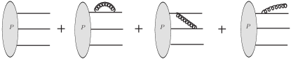
Figure 2: Diagrammatic representation of the proton state $|P\rangle$ up to NLO.

At LO the proton state on the light cone is approximated by a three-quark Fock state with the wave function $\Psi_{qqq}(x_{1},\vec{k}_{1};x_{2},\vec{k}_{2};x_{3},\vec{k}_{3})$ Brodsky:1997de ; Schlumpf:1992vq ; Brodsky:1994fz . Here, $\vec{k}_{i}$ are the transverse momenta of the on-shell quarks in the transverse rest frame of the proton. At NLO, there are ${\cal O}(g)$ corrections due to the emission of a gluon by one of the quarks as well as ${\cal O}(g^{2})$ virtual corrections due to the exchange of a gluon by a quark either with itself or with another quark. This is shown in Fig. 2; explicit expressions are given in Ref. Dumitru:2020gla .

The valence quark wave function $\Psi_{qqq}$ is gauge invariant and universal, process independent. It encodes the non-perturbative structure of the proton at low transverse momentum scales, and light cone momentum fraction in the valence quark regime. For our numerical estimates here, we employ a simple model due to Brodsky and Schlumpf Brodsky:1994fz

$$\Psi_{qqq}=N_{\mathrm{HO}}\sqrt{x_{1}x_{2}x_{3}}\prod_{i=1}^{3}\exp\left(-\frac{(\vec{k}_{i}^{2}+M^{2})/x_{i}}{2\beta^{2}}\right).$$ (8)

This “harmonic oscillator” wave function is our default choice. For some observables we have also checked the power-law wave function

$$\Psi_{qqq}=N_{\mathrm{p}}\sqrt{x_{1}x_{2}x_{3}}\left(1+\sum_{i=1}^{3}\frac{\vec{k}_{i}^{2}+\tilde{M}^{2}}{x_{i}\tilde{\beta}^{2}}\right)^{-p}.$$ (9)

The non-perturbative parameters $M=0.26\,\mathrm{GeV}$ and $\beta=0.55\,\mathrm{GeV}$, introduced in Eq. (8), have been tuned in Ref. Brodsky:1994fz to reproduce the radius, the anomalous magnetic moment, and the axial coupling of the proton and the neutron. Similarly parameters for the power-law wave function (9) are available in Ref. Brodsky:1994fz . Note that because of the constraints that $x_{1}+x_{2}+x_{3}=1$ and $\vec{k}_{1}+\vec{k}_{2}+\vec{k}_{3}=0$, the proton state also encodes longitudinal and transverse momentum correlations among the quarks.

We have observed rather small differences in the kinematic regimes covered by the figures below. We therefore do not show explicitly the results corresponding to the power law valence quark wave function. The normalization factor of $\Psi_{qqq}$ is obtained from the requirement that the states are normalized as

$$\langle K|P\rangle = 16\pi^{3}\,P^{+}\,\delta(P^{+}-K^{+})\,\delta(\vec{P}-\vec{K})$$ (10)

$$\to \frac{1}{2}\int[\mathrm{d}x_{i}]\int[\mathrm{d}^{2}\vec{k}_{i}]\,\,|\Psi_{qqq}(x_{i},\vec{k}_{i})|^{2}=1,$$

where the phase space factors are defined as:

$$[\mathrm{d}x_{i}] \equiv \frac{\mathrm{d}x_{1}\mathrm{d}x_{2}\mathrm{d}x_{3}}{8x_{1}x_{2}x_{3}}\,\delta(1-x_{1}-x_{2}-x_{3}),$$ (11)

$$\left[\mathrm{d}^{2}\vec{k}_{i}\right] \equiv \frac{\mathrm{d}^{2}\vec{k}_{1}\mathrm{d}^{2}\vec{k}_{2}\mathrm{d}^{2}\vec{k}_{3}}{(2\pi)^{6}}\,\delta(\vec{k}_{1}+\vec{k}_{2}+\vec{k}_{3}).$$ (12)

Other models for the valence quark wave functions include those of Refs. Frank:1995pv ; Miller:2002ig ; Pasquini:2007iz ; Pasquini:2009bv ; Lorce:2011dv . Valence quark wave functions have also been obtained numerically by solving various model Hamiltonians Zhao:2020gtf ; Xu:2020xbt ; Mondal:2020mpv .

IV Results and discussion

For all numerical results we use fixed coupling $\alpha_{\mathrm{s}}=0.2$. We note that NLO corrections increase relative to the LO results in proportion to $\alpha_{\mathrm{s}}$. Also, unless mentioned otherwise, our default choice for the collinear cutoff is $m=0.2$ GeV. We show results at different $x$, which is the lower cutoff for the emitted gluon longitudinal momentum in the NLO diagrams. We also use $x$ as a lower limit in the integrations over the valence quark momentum fractions $x_{i}$.

IV.1 Color charge density correlator

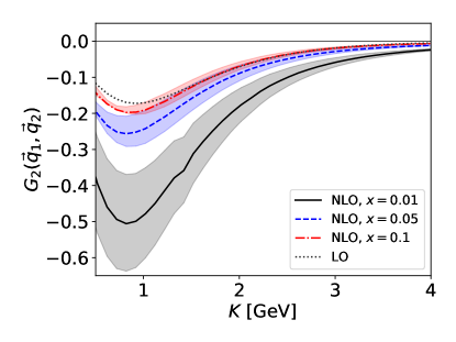
Figure 3: Color charge correlator in momentum space at different $x$ for the configuration where $\vec{q}_{1}=\vec{q}_{2}=(K/2,0)$ are parallel. The results are shown in the perturbative $K>0.5\,\mathrm{GeV}$ region. The bands correspond to the variation of the collinear cutoff in $m=0.1\,\mathrm{GeV}\dots 0.4\,\mathrm{GeV}$.

To study the magnitude of the NLO correction, we evaluate the two point function $G_{2}(\vec{q}_{1},\vec{q}_{2})$ in momentum space. We first choose a configuration where the two probe gluons carry the same momentum, $\vec{q}_{1}=\vec{q}_{2}=(K/2,0)$. Note that here, and in the following discussion, we use the notation $K=|\vec{K}|$ for the length of all transverse vectors. The color charge correlator as a function of the transverse momentum transfer $K$ is shown in Fig. 3. The leading order result is compared to the full NLO result (which also includes the leading order $\sim g^{2}$ contribution) obtained with three different values for the momentum cutoff $x$. As expected, the one gluon emission correction grows rapidly with decreasing $x$, and completely dominates at $x=0.01$. At greater $x=0.05$ the NLO correction is comparable to the leading order contribution, to finally become a small correction at $x=0.1$. The fact that the perturbative correction is numerically small at $x=0.1$ represents a non-trivial consistency check of the ”expansion” about the LO three-quark state. We also observe that the dependence on the collinear cutoff $m$ is moderate, as is the case in all results shown in this Section.

We have mentioned above that at leading order, the configuration with approximately equal momenta is dominated by the cat’s ears diagram, which corresponds to the matrix element of a two-body operator and gives a negative contribution to $G_{2}$. The figure shows that the correlation function for $\vec{q}_{1}=\vec{q}_{2}$ remains negative, i.e. dominated by two-body correlations, even in the regime of small $x$ where the NLO correction is greater than the LO contribution.

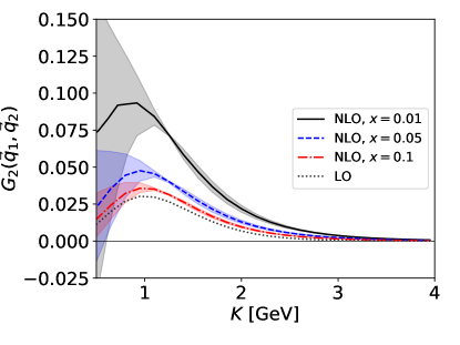
Figure 4: Color charge correlator in momentum space at different $x$ for the configuration where the probe momenta are perpendicular: $\vec{q}_{1}=(K/\sqrt{2},0)$ and $\vec{q}_{2}=(0,K/\sqrt{2})$, so $q_{12}=K$. The results are shown in the perturbative $K>0.5\,\mathrm{GeV}$ region. The bands correspond to the variation of the collinear cutoff in $m=0.1\,\mathrm{GeV}\dots 0.4\,\mathrm{GeV}$.

In Fig. 4 we show $G_{2}(\vec{q}_{1},\vec{q}_{2})$ for perpendicular momenta where contributions of hand-bag type are less suppressed. Indeed, the correlator is now positive, although this contribution is generically smaller in magnitude than the negative contribution from the cat’s ears type diagrams shown in the previous Fig. 3. The NLO correction amounts to stronger positive correlations at all momentum transfers $K$. At small $K\lesssim 1\,\mathrm{GeV}$ the results depend strongly on the value chosen for the collinear cutoff $m$. Of course, at small $K$ and small $q_{12}$ the perturbative computation of the color charge correlator in terms of two gluon exchange should be interpreted with caution.

We now proceed to show the color charge correlator $G_{2}(\vec{q}_{12},\vec{b})$ in mixed transverse momentum - transverse coordinate space, c.f. Fig. 5.

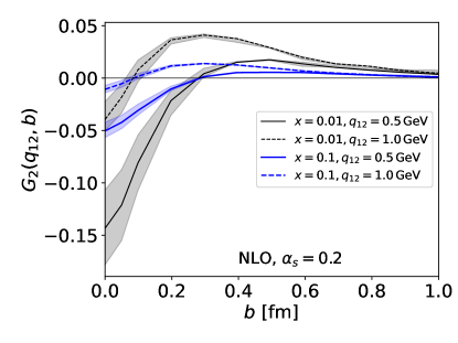
Figure 5: Color charge correlator $G_{2}(\vec{q}_{12},\vec{b})$ as a function of impact parameter for various relative transverse momenta $q_{12}$ averaged over the angle between $\vec{q}_{12}$ and $\vec{b}$. The bands correspond to the variation of the collinear cutoff in $m=0.1\,\mathrm{GeV}\dots 0.4\,\mathrm{GeV}$.

Near the center of the proton at small $b$ we find that $G_{2}<0$; “repulsive” two-body correlations dominate here. Also, comparing $x=0.1$ to $x=0.01$ we note that the NLO correction mainly affects $G_{2}$ at small $b$ to strongly boost these negative two-body correlations, more so for smaller $q_{12}$. However, hand-bag type contributions become more prominent with increasing $q_{12}$ or $b$. At small $x=0.01$ and large $q_{12}=1$ GeV, we observe that significant positive color charge correlations emerge for impact parameters $b\gtrsim 0.2$ fm. Generically, the large-$b$ tails of the two-point correlator $G_{2}$ exhibit a fall-off that resembles a transverse profile function. Here, the one gluon emission NLO correction is in line with the simple intuitive picture whereby it increases the mean square color charge density. However, there is a large negative correction near the center of the proton.

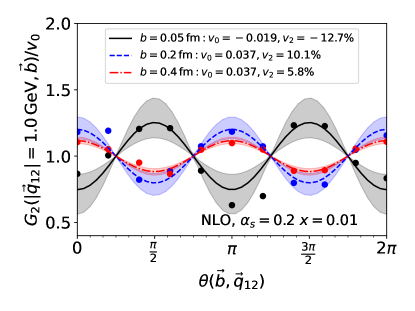
Figure 6: $G_{2}(\vec{q}_{12},\vec{b})$ as a function of the azimuthal angle made by $\vec{q}_{12}$ and $\vec{b}$ at three different impact parameters. Curves show fits of the form $v_{0}(1+2v_{2}\cos 2\theta$). The bands correspond to the variation of the collinear cutoff in $m=0.1\,\mathrm{GeV}\dots 0.4\,\mathrm{GeV}$.

The charge correlator in the MV model, even in its modified version with a non-trivial shape function, is independent of the relative transverse momentum $\vec{q}_{12}$ and its angular orientation relative to the impact parameter vector $\vec{b}$. We have already documented above the dependence of our result for $G_{2}$ on the magnitude of $\vec{q}_{12}$. Fig. 6 shows that it depends also on the relative azimuthal orientation $\theta$ of these vectors. We observe a $\sim\cos 2(\theta-\varphi)$ azimuthal anisotropy in $G_{2}$ normalized by its angular average. The phase shift is $\varphi=0$ in the kinematic regime where the correlator is positive, and $\varphi=\pi/2$ in the regime dominated by “repulsive” correlations where $G_{2}(\vec{q}_{12},\vec{b})<0$.

IV.2 Dipole scattering amplitude $N(\vec{r},\vec{b})$

In this section, we document the ”evolution” of the dipole scattering amplitude from $x=0.1$ to $x=0.01$, and its angular dependence. We have not attempted to tune the coupling constant or the quark mass collinear cutoff to data from inclusive DIS or exclusive $J/\Psi$ production; detailed studies of phenomenological predictions are left for the future.

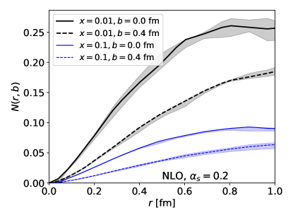
Figure 7: Dipole scattering amplitude at NLO as a function of dipole size $r$ at impact parameters $b=0$ and at $b=0.4\,\mathrm{fm}$ at two different $x$ averaged over the angle between $\vec{r}$ and $\vec{b}$. The bands correspond to the variation of the collinear cutoff in $m=0.1\,\mathrm{GeV}\dots 0.4\,\mathrm{GeV}$.

In Fig. 7 we show the evolution of the dipole scattering amplitude from $x=0.1$ to $x=0.01$, at two different impact parameters. We observe much stronger scattering at higher energy (lower $x$) by a factor of $\approx 3$, even though $\alpha_{s}\log\frac{0.1}{0.01}=0.46$ is not a big number. However, there are many diagrams for NLO corrections. The obtained dipole amplitude $N(\vec{r},\vec{b};x)$ can be directly used as an initial condition for the (impact parameter dependent) BK evolution studied e.g. in Refs. GolecBiernat:2003ym ; Berger:2010sh ; Berger:2011ew ; Berger:2012wx ; Cepila:2018faq ; Bendova:2019psy ; Cepila:2020xol ; Bendova:2020hkp .

We continue with an analysis of the azimuthal anisotropy of the dipole scattering amplitude. If the color charge correlator is taken to be isotropic and proportional to the shape function of the target then, in the two-gluon exchange approximation at small $r$ and $b$,

$$N(\vec{r},\vec{b})=f(r,b)\,\left[1+c\,(rb)^{2}\cos 2\theta\right].$$ (13)

Here, the function $f(r,b)$ is independent of the angle $\theta$ between $\vec{r}$ and $\vec{b}$, and $c>0$ is a constant with mass dimension 4. See Ref. Iancu:2017fzn for a derivation of this result, and Fig. 18 in Ref. Mantysaari:2020lhf for a nice graphical representation. Here, the angular dependence arises due to the fact that under rotations of the dipole at fixed $\vec{b}$ its endpoints probe different “densities” in the target, when its transverse profile function is not constant. (The target is isotropic only w.r.t. its center but is not invariant under rotations about the displaced point $\vec{b}$). Eq. (13) predicts a $\sim\cos 2\theta$ azimuthal dependence with an amplitude proportional to the squares of the size of the dipole and of the impact parameter.

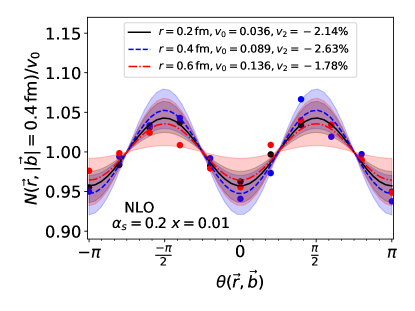
Figure 8: Dipole scattering amplitude at NLO as a function of the angle between $\vec{r}$ and $\vec{b}$. Points show the actual result of a numerical calculation and lines are obtained by fitting a functional form $v_{0}(1+2v_{2}\cos 2\theta)$. The bands correspond to the variation of the collinear cutoff in $m=0.1\,\mathrm{GeV}\dots 0.4\,\mathrm{GeV}$.

Figure 8 shows our result for $N(\vec{r},\vec{b})$ at fixed $b=0.4$ fm. It indeed displays a $\sim\cos 2\theta$ azimuthal dependence, but in contrast to MV model based calculations of Refs. Iancu:2017fzn ; Mantysaari:2019csc ; Mantysaari:2020lhf we find a phase shift of $\pi/2$, i.e. a negative $v_{2}=\langle\cos 2\theta\rangle$ (or $c<0$ in Eq. (13)). Physically, our result corresponds to stronger scattering when the dipole is oriented perpendicular to the impact parameter. In the calculations based on the MV model one finds the opposite behavior where parallel alignment results in a greater scattering amplitude. At the given impact parameter, we find that the amplitude of the angular modulation is nearly constant for $r=0.2\dots 0.6$ fm. This indicates that the non-zero $\langle\cos 2\theta\rangle$ is not entirely due to simply a non-trivial shape function of the target proton. Indeed, the angular dependence of the color charge correlator itself, which we have shown in the previous section, is also important. The nearly constant $v_{2}$ when $r=0.2\to 0.6~{}\mathrm{fm}$ may support the “domain” picture introduced by Kovner and Lublinsky Kovner:2012jm .

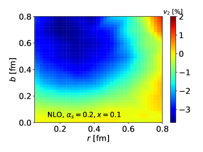
Figure 9: $v_{2}=\langle\cos 2\theta\rangle$ from the dipole scattering amplitude at NLO in the impact parameter vs. dipole size plane at $x=0.1$. The smallest dipole size at the left edge of the plot is $r_{\text{min}}=0.05~{}\mathrm{fm}.$

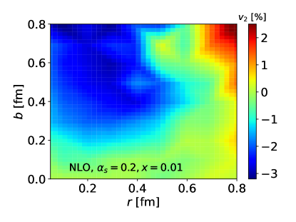
Figure 10: $v_{2}=\langle\cos 2\theta\rangle$ from the dipole scattering amplitude at NLO in the impact parameter vs. dipole size plane at $x=0.01$. The smallest dipole size at the left edge of the plot is $r_{\text{min}}=0.05~{}\mathrm{fm}.$

The amplitudes $v_{2}=\langle\cos 2\theta\rangle$ of the azimuthal modulation in the $b$ vs. $r$ plane at $x=0.1$ and at $x=0.01$ are shown in Figs. 9 and 10. Here, we observe a rather mild modification of the azimuthal asymmetry with decreasing $x$. Although the NLO effects dominate the scattering amplitude at $x=0.01$ (as shown above), the azimuthal amplitude $v_{2}$ does not depend strongly on the momentum fraction $x$, and consequently the NLO corrections have a small effect on $v_{2}$. The fact that $v_{2}$ is approximately independent of $r$ at $r\lesssim 0.5$ fm can be clearly seen from these figures. We find $v_{2}<0$ in the region of $r,b$ where the perturbative calculation is reliable. In particular, the dependence on the dipole size $r$ is completely different to what is obtained from the impact parameter dependent MV model shown in Eq. (13) and numerically studied in Ref. Mantysaari:2020lhf .

V Summary and Outlook

In this Letter, we have computed and shown the behavior of color charge correlations (at quadratic order in $\rho^{a}$) in a proton on the light cone. At LO the proton is approximated by a three quark state with a wave function that is consistent with its empirically observed structure at large $x$ Schlumpf:1992vq ; Brodsky:1994fz , which we refine by including NLO corrections due to emission or exchange of a perturbative gluon. Our results apply in a regime of moderately high energy, perhaps corresponding to light cone momentum fractions of $x=0.01\ldots 0.1$, where scattering is approximately eikonal but still far from the unitarity limit.

We have emphasized that the correlator exhibits non-trivial behavior at large momentum transfer or central impact parameters. In that regime, it does not merely trace the behavior of a transverse proton shape function but displays repulsive correlations due to the “cat’s ears diagram” at leading order, which persist at next-to-leading order. Furthermore, the color charge correlation function depends not only on the impact parameter $\vec{b}$ but also on the relative transverse momentum $\vec{q}_{12}$ of the two gluon probes, and on the angle made by $\vec{b}$ and $\vec{q}_{12}$. This is in contrast to the McLerran-Venugopalan (MV) model McLerran:1993ni ; McLerran:1993ka , which is used extensively in the literature.

Furthermore, from the two-point color charge correlator, we have computed the dipole scattering amplitude $N(\vec{r},\vec{b};x)$ in the two gluon exchange approximation. This includes the contributions from the soft and collinear singularities without restriction to the leading logarithmic approximation. We observe a strong amplification of color charge density fluctuations with decreasing $x$; from $x=0.1$ to $x=0.01$ the dipole scattering amplitude $N(\vec{r},\vec{b};x)$ increases by factors of $\sim 3$ (for $\alpha_{\mathrm{s}}=0.2$). We also find that the azimuthal anisotropy of the dipole scattering amplitude is affected significantly by the angular dependence of the color charge correlations. We observe a behavior of $\langle\cos 2\theta\rangle$ which, in some ranges of impact parameter and dipole size, differs substantially from expectations based on isotropic color charge correlators proportional to the proton profile function $T_{p}(b)$ Altinoluk:2015dpi ; Iancu:2017fzn ; Mantysaari:2019csc ; Mantysaari:2020lhf .

Our computations also provide initial conditions for Balitsky-Kovchegov (BK) evolution of the dipole scattering amplitude to lower $x$ Balitsky:1995ub ; Kovchegov:1999yj ; Ducloue:2019ezk ; in particular, for impact parameter dependent evolution GolecBiernat:2003ym ; Berger:2010sh ; Berger:2011ew ; Berger:2012wx ; Cepila:2018faq ; Bendova:2019psy ; Cepila:2020xol ; Bendova:2020hkp . This initial condition depends not only on the impact parameter and the dipole vectors but also on their relative angle, and on the light-cone momentum fraction $x$ in the target. In the future, proton “imaging” in the regime of small and moderate $x$ performed at the EIC Boer:2011fh ; Accardi:2012qut ; Aschenauer:2017jsk ; AbdulKhalek:2021gbh , at other future nuclear DIS facilities Agostini:2020fmq ; Anderle:2021wcy or in ultra peripheral collisions Bertulani:2005ru ; Klein:2019qfb at the LHC, will further constrain the proton light cone wave function, and the dipole scattering amplitude which we relate to it.

We close with a brief outlook. We have already mentioned the successful phenomenology that emerged from the picture of a fluctuating proton substructure Mantysaari:2016ykx ; Mantysaari:2016jaz ; Mantysaari:2017dwh ; Mantysaari:2017cni ; Albacete:2016pmp ; Albacete:2016gxu ; Cepila:2016uku ; Cepila:2017nef ; Albacete:2017ajt ; Traini:2018hxd ; Mantysaari:2018zdd ; Moreland:2018gsh ; Mantysaari:2019jhh (see Mantysaari:2020axf for a review). It will be very interesting to reformulate these approaches so that the ensemble of quark and gluon configurations in the proton would be determined by its light cone wave function at NLO rather than be based on geometric pictures.

References

- (1) D. Boer et. al., Gluons and the quark sea at high energies: Distributions, polarization, tomography, arXiv:1108.1713 [nucl-th].
- (2) A. Accardi et. al., Electron Ion Collider: The Next QCD Frontier: Understanding the glue that binds us all, Eur. Phys. J. A 52 (2016) no. 9 268 [arXiv:1212.1701 [nucl-ex]].
- (3) E. C. Aschenauer, S. Fazio, J. H. Lee, H. Mäntysaari, B. S. Page, B. Schenke, T. Ullrich, R. Venugopalan and P. Zurita, The electron–ion collider: assessing the energy dependence of key measurements, Rept. Prog. Phys. 82 (2019) no. 2 024301 [arXiv:1708.01527 [nucl-ex]].
- (4) R. Abdul Khalek et. al., Science Requirements and Detector Concepts for the Electron-Ion Collider: EIC Yellow Report, arXiv:2103.05419 [physics.ins-det].
- (5) LHeC and FCC-he Study Group collaboration, P. Agostini et. al., The Large Hadron-Electron Collider at the HL-LHC, arXiv:2007.14491 [hep-ex].
- (6) D. P. Anderle et. al., Electron-Ion Collider in China, arXiv:2102.09222 [nucl-ex].
- (7) M. Burkardt, Quark correlations and single spin asymmetries, Phys. Rev. D 69 (2004) 057501 [arXiv:hep-ph/0311013].
- (8) C. Lorce and B. Pasquini, Quark Wigner Distributions and Orbital Angular Momentum, Phys. Rev. D 84 (2011) 014015 [arXiv:1106.0139 [hep-ph]].
- (9) A. V. Belitsky, X.-d. Ji and F. Yuan, Quark imaging in the proton via quantum phase space distributions, Phys. Rev. D 69 (2004) 074014 [arXiv:hep-ph/0307383].
- (10) X.-d. Ji, Viewing the proton through ’color’ filters, Phys. Rev. Lett. 91 (2003) 062001 [arXiv:hep-ph/0304037].
- (11) Y. Hatta, B.-W. Xiao and F. Yuan, Probing the Small- x Gluon Tomography in Correlated Hard Diffractive Dijet Production in Deep Inelastic Scattering, Phys. Rev. Lett. 116 (2016) no. 20 202301 [arXiv:1601.01585 [hep-ph]].
- (12) Y. Hatta, B.-W. Xiao and F. Yuan, Gluon Tomography from Deeply Virtual Compton Scattering at Small-x, Phys. Rev. D 95 (2017) no. 11 114026 [arXiv:1703.02085 [hep-ph]].
- (13) H. Mäntysaari, K. Roy, F. Salazar and B. Schenke, Gluon imaging using azimuthal correlations in diffractive scattering at the Electron-Ion Collider, arXiv:2011.02464 [hep-ph].
- (14) H. Mäntysaari, N. Mueller and B. Schenke, Diffractive Dijet Production and Wigner Distributions from the Color Glass Condensate, Phys. Rev. D 99 (2019) no. 7 074004 [arXiv:1902.05087 [hep-ph]].
- (15) A. Dumitru and R. Paatelainen, Sub-femtometer scale color charge fluctuations in a proton made of three quarks and a gluon, Phys. Rev. D 103 (2021) no. 3 034026 [arXiv:2010.11245 [hep-ph]].
- (16) A. Dumitru, V. Skokov and T. Stebel, Subfemtometer scale color charge correlations in the proton, Phys. Rev. D 101 (2020) no. 5 054004 [arXiv:2001.04516 [hep-ph]].
- (17) A. Dumitru, G. A. Miller and R. Venugopalan, Extracting many-body color charge correlators in the proton from exclusive DIS at large Bjorken x, Phys. Rev. D 98 (2018) no. 9 094004 [arXiv:1808.02501 [hep-ph]].
- (18) L. D. McLerran and R. Venugopalan, Computing quark and gluon distribution functions for very large nuclei, Phys. Rev. D 49 (1994) 2233 [arXiv:hep-ph/9309289].
- (19) L. D. McLerran and R. Venugopalan, Gluon distribution functions for very large nuclei at small transverse momentum, Phys. Rev. D 49 (1994) 3352 [arXiv:hep-ph/9311205].
- (20) J. L. Albacete and A. Soto-Ontoso, Hot spots and the hollowness of proton–proton interactions at high energies, Phys. Lett. B 770 (2017) 149 [arXiv:1605.09176 [hep-ph]].
- (21) J. L. Albacete, H. Petersen and A. Soto-Ontoso, Correlated wounded hot spots in proton-proton interactions, Phys. Rev. C 95 (2017) no. 6 064909 [arXiv:1612.06274 [hep-ph]].
- (22) J. L. Albacete, H. Petersen and A. Soto-Ontoso, Symmetric cumulants as a probe of the proton substructure at LHC energies, Phys. Lett. B 778 (2018) 128 [arXiv:1707.05592 [hep-ph]].
- (23) H1 and ZEUS collaboration, H. Abramowicz et. al., Combination of measurements of inclusive deep inelastic scattering cross sections and QCD analysis of HERA data, Eur. Phys. J. C 75 (2015) no. 12 580 [arXiv:1506.06042 [hep-ex]].
- (24) E. Iancu and R. Venugopalan, The Color glass condensate and high-energy scattering in QCD, pp. 249–363. World Scientific, 2003. arXiv:hep-ph/0303204.
- (25) A. Kovner, High energy evolution: The Wave function point of view, Acta Phys. Polon. B 36 (2005) 3551 [arXiv:hep-ph/0508232].
- (26) F. Gelis, E. Iancu, J. Jalilian-Marian and R. Venugopalan, The Color Glass Condensate, Ann. Rev. Nucl. Part. Sci. 60 (2010) 463 [arXiv:1002.0333 [hep-ph]].
- (27) J.-P. Blaizot, High gluon densities in heavy ion collisions, Rept. Prog. Phys. 80 (2017) no. 3 032301 [arXiv:1607.04448 [hep-ph]].
- (28) Y. V. Kovchegov, Small structure function of a nucleus including multiple pomeron exchanges, Phys. Rev. D 60 (1999) 034008 [arXiv:hep-ph/9901281].
- (29) I. Balitsky, Operator expansion for high-energy scattering, Nucl. Phys. B 463 (1996) 99 [arXiv:hep-ph/9509348].
- (30) J. L. Albacete, N. Armesto, J. G. Milhano, P. Quiroga-Arias and C. A. Salgado, AAMQS: A non-linear QCD analysis of new HERA data at small-x including heavy quarks, Eur. Phys. J. C 71 (2011) 1705 [arXiv:1012.4408 [hep-ph]].
- (31) T. Lappi and H. Mäntysaari, Single inclusive particle production at high energy from HERA data to proton-nucleus collisions, Phys. Rev. D 88 (2013) 114020 [arXiv:1309.6963 [hep-ph]].
- (32) G. Beuf, H. Hänninen, T. Lappi and H. Mäntysaari, Color Glass Condensate at next-to-leading order meets HERA data, Phys. Rev. D 102 (2020) 074028 [arXiv:2007.01645 [hep-ph]].
- (33) G. Beuf, Improving the kinematics for low- QCD evolution equations in coordinate space, Phys. Rev. D 89 (2014) no. 7 074039 [arXiv:1401.0313 [hep-ph]].
- (34) B. Ducloué, E. Iancu, A. Mueller, G. Soyez and D. Triantafyllopoulos, Non-linear evolution in QCD at high-energy beyond leading order, JHEP 04 (2019) 081 [arXiv:1902.06637 [hep-ph]].
- (35) R. Boussarie and Y. Mehtar-Tani, A novel formulation of the unintegrated gluon distribution for DIS, arXiv:2006.14569 [hep-ph].
- (36) T. Lappi, H. Mäntysaari and J. Penttala, Relativistic corrections to the vector meson light front wave function, Phys. Rev. D 102 (2020) no. 5 054020 [arXiv:2006.02830 [hep-ph]].
- (37) B. Ducloué, H. Hänninen, T. Lappi and Y. Zhu, Deep inelastic scattering in the dipole picture at next-to-leading order, Phys. Rev. D 96 (2017) no. 9 094017 [arXiv:1708.07328 [hep-ph]].
- (38) T. Lappi and H. Mäntysaari, Direct numerical solution of the coordinate space Balitsky-Kovchegov equation at next to leading order, Phys. Rev. D 91 (2015) no. 7 074016 [arXiv:1502.02400 [hep-ph]].
- (39) T. Lappi and H. Mäntysaari, Next-to-leading order Balitsky-Kovchegov equation with resummation, Phys. Rev. D 93 (2016) no. 9 094004 [arXiv:1601.06598 [hep-ph]].
- (40) H. Hänninen, T. Lappi and R. Paatelainen, One-loop corrections to light cone wave functions: the dipole picture DIS cross section, Annals Phys. 393 (2018) 358 [arXiv:1711.08207 [hep-ph]].
- (41) T. Lappi and R. Paatelainen, The one loop gluon emission light cone wave function, Annals Phys. 379 (2017) 34 [arXiv:1611.00497 [hep-ph]].
- (42) R. Boussarie, A. Grabovsky, D. Y. Ivanov, L. Szymanowski and S. Wallon, Next-to-Leading Order Computation of Exclusive Diffractive Light Vector Meson Production in a Saturation Framework, Phys. Rev. Lett. 119 (2017) no. 7 072002 [arXiv:1612.08026 [hep-ph]].
- (43) M. A. Escobedo and T. Lappi, Dipole picture and the nonrelativistic expansion, Phys. Rev. D 101 (2020) no. 3 034030 [arXiv:1911.01136 [hep-ph]].
- (44) G. Beuf, Dipole factorization for DIS at NLO: Loop correction to the light-front wave functions, Phys. Rev. D 94 (2016) no. 5 054016 [arXiv:1606.00777 [hep-ph]].
- (45) T. Altinoluk and A. Kovner, Particle Production at High Energy and Large Transverse Momentum - ’The Hybrid Formalism’ Revisited, Phys. Rev. D 83 (2011) 105004 [arXiv:1102.5327 [hep-ph]].
- (46) T. Altinoluk, N. Armesto, G. Beuf, A. Kovner and M. Lublinsky, Single-inclusive particle production in proton-nucleus collisions at next-to-leading order in the hybrid formalism, Phys. Rev. D 91 (2015) no. 9 094016 [arXiv:1411.2869 [hep-ph]].
- (47) K. Roy and R. Venugopalan, NLO impact factor for inclusive photondijet production in DIS at small , Phys. Rev. D 101 (2020) no. 3 034028 [arXiv:1911.04530 [hep-ph]].
- (48) A. Dumitru and T. Stebel, Multiquark matrix elements in the proton and three gluon exchange for exclusive production in photon-proton diffractive scattering, Phys. Rev. D 99 (2019) no. 9 094038 [arXiv:1903.07660 [hep-ph]].
- (49) J. Bartels and C. Ewerz, Unitarity corrections in high-energy QCD, JHEP 09 (1999) 026 [arXiv:hep-ph/9908454].
- (50) C. Ewerz, Reggeization in high-energy QCD, JHEP 04 (2001) 031 [arXiv:hep-ph/0103260].
- (51) Y. V. Kovchegov, NonAbelian Weizsacker-Williams field and a two-dimensional effective color charge density for a very large nucleus, Phys. Rev. D 54 (1996) 5463 [arXiv:hep-ph/9605446].
- (52) B. Schenke, P. Tribedy and R. Venugopalan, Event-by-event gluon multiplicity, energy density, and eccentricities in ultrarelativistic heavy-ion collisions, Phys. Rev. C 86 (2012) 034908 [arXiv:1206.6805 [hep-ph]].
- (53) B. Schenke, P. Tribedy and R. Venugopalan, Fluctuating Glasma initial conditions and flow in heavy ion collisions, Phys. Rev. Lett. 108 (2012) 252301 [arXiv:1202.6646 [nucl-th]].
- (54) E. Iancu and A. H. Rezaeian, Elliptic flow from color-dipole orientation in pp and pA collisions, Phys. Rev. D 95 (2017) no. 9 094003 [arXiv:1702.03943 [hep-ph]].
- (55) A. Kovner and V. V. Skokov, Does shape matter? vs eccentricity in small x gluon production, Phys. Lett. B 785 (2018) 372 [arXiv:1805.09297 [hep-ph]].
- (56) H. Mäntysaari and B. Schenke, Accessing the gluonic structure of light nuclei at a future electron-ion collider, Phys. Rev. C 101 (2020) no. 1 015203 [arXiv:1910.03297 [hep-ph]].
- (57) H. Mäntysaari and B. Schenke, Confronting impact parameter dependent JIMWLK evolution with HERA data, Phys. Rev. D 98 (2018) no. 3 034013 [arXiv:1806.06783 [hep-ph]].
- (58) H. Mäntysaari and B. Schenke, Evidence of strong proton shape fluctuations from incoherent diffraction, Phys. Rev. Lett. 117 (2016) no. 5 052301 [arXiv:1603.04349 [hep-ph]].
- (59) H. Mäntysaari and B. Schenke, Revealing proton shape fluctuations with incoherent diffraction at high energy, Phys. Rev. D 94 (2016) no. 3 034042 [arXiv:1607.01711 [hep-ph]].
- (60) S. Demirci, T. Lappi and S. Schlichting, Hot spots and gluon field fluctuations as causes of eccentricity in small systems, arXiv:2101.03791 [hep-ph].
- (61) S. J. Brodsky, H.-C. Pauli and S. S. Pinsky, Quantum chromodynamics and other field theories on the light cone, Phys. Rept. 301 (1998) 299 [arXiv:hep-ph/9705477].
- (62) F. Schlumpf, Relativistic constituent quark model of electroweak properties of baryons, Phys. Rev. D 47 (1993) 4114 [arXiv:hep-ph/9212250]. [Erratum: Phys.Rev.D 49, 6246 (1994)].
- (63) S. J. Brodsky and F. Schlumpf, Wave function independent relations between the nucleon axial coupling and the nucleon magnetic moments, Phys. Lett. B 329 (1994) 111 [arXiv:hep-ph/9402214].
- (64) M. Frank, B. Jennings and G. Miller, The Role of color neutrality in nuclear physics: Modifications of nucleonic wave functions, Phys. Rev. C 54 (1996) 920 [arXiv:nucl-th/9509030].
- (65) G. A. Miller, Light front cloudy bag model: Nucleon electromagnetic form-factors, Phys. Rev. C 66 (2002) 032201 [arXiv:nucl-th/0207007].
- (66) B. Pasquini and S. Boffi, Electroweak structure of the nucleon, meson cloud and light-cone wavefunctions, Phys. Rev. D 76 (2007) 074011 [arXiv:0707.2897 [hep-ph]].
- (67) B. Pasquini, S. Boffi and P. Schweitzer, The Spin Structure of the Nucleon in Light-Cone Quark Models, Mod. Phys. Lett. A 24 (2009) 2903 [arXiv:0910.1677 [hep-ph]].
- (68) C. Lorce, B. Pasquini and M. Vanderhaeghen, Unified framework for generalized and transverse-momentum dependent parton distributions within a 3Q light-cone picture of the nucleon, JHEP 05 (2011) 041 [arXiv:1102.4704 [hep-ph]].
- (69) BLFQ collaboration, X. Zhao, K. Fu, H. Zhao, J. Lan, C. Mondal, S. Xu and J. P. Vary in 18th International Conference on Hadron Spectroscopy and Structure, pp. 624–631, 2020. arXiv:2004.02456 [nucl-th].
- (70) BLFQ collaboration, S. Xu, C. Mondal, J. Lan, X. Zhao, Y. Li and J. P. Vary in 18th International Conference on Hadron Spectroscopy and Structure, pp. 607–611, 2020. arXiv:2004.02464 [hep-ph].
- (71) C. Mondal, S. Xu, J. Lan, X. Zhao, Y. Li, D. Chakrabarti and J. P. Vary, Basis light-front quantization approach to nucleon, PoS LC2019 (2020) 067 [arXiv:2001.04414 [hep-ph]].
- (72) K. J. Golec-Biernat and A. Stasto, On solutions of the Balitsky-Kovchegov equation with impact parameter, Nucl. Phys. B 668 (2003) 345 [arXiv:hep-ph/0306279].
- (73) J. Berger and A. Stasto, Numerical solution of the nonlinear evolution equation at small x with impact parameter and beyond the LL approximation, Phys. Rev. D 83 (2011) 034015 [arXiv:1010.0671 [hep-ph]].
- (74) J. Berger and A. M. Stasto, Small nonlinear evolution with impact parameter and the structure function data, Phys. Rev. D 84 (2011) 094022 [arXiv:1106.5740 [hep-ph]].
- (75) J. Berger and A. M. Stasto, Exclusive vector meson production and small- evolution, JHEP 01 (2013) 001 [arXiv:1205.2037 [hep-ph]].
- (76) J. Cepila, J. Contreras and M. Matas, Collinearly improved kernel suppresses Coulomb tails in the impact-parameter dependent Balitsky-Kovchegov evolution, Phys. Rev. D 99 (2019) no. 5 051502 [arXiv:1812.02548 [hep-ph]].
- (77) D. Bendova, J. Cepila, J. Contreras and M. Matas, Solution to the Balitsky-Kovchegov equation with the collinearly improved kernel including impact-parameter dependence, Phys. Rev. D 100 (2019) no. 5 054015 [arXiv:1907.12123 [hep-ph]].
- (78) J. Cepila, J. Contreras and M. Matas, Predictions for nuclear structure functions from the impact-parameter dependent Balitsky-Kovchegov equation, Phys. Rev. C 102 (2020) no. 4 044318 [arXiv:2002.11056 [hep-ph]].
- (79) D. Bendova, J. Cepila, J. Contreras, t. V. Gonçalves and M. Matas, Diffractive deeply inelastic scattering in future electron-ion colliders, arXiv:2009.14002 [hep-ph].
- (80) E. Levin and A. H. Rezaeian, The Ridge from the BFKL evolution and beyond, Phys. Rev. D 84 (2011) 034031 [arXiv:1105.3275 [hep-ph]].
- (81) A. Kovner and M. Lublinsky, Angular and long range rapidity correlations in particle production at high energy, Int. J. Mod. Phys. E 22 (2013) 1330001 [arXiv:1211.1928 [hep-ph]].
- (82) B. Kopeliovich, H. Pirner, A. Rezaeian and I. Schmidt, Azimuthal anisotropy of direct photons, Phys. Rev. D 77 (2008) 034011 [arXiv:0711.3010 [hep-ph]].
- (83) B. Kopeliovich, A. Rezaeian and I. Schmidt, Azimuthal Asymmetry of pions in pp and pA collisions, Phys. Rev. D 78 (2008) 114009 [arXiv:0809.4327 [hep-ph]].
- (84) J. Zhou, Elliptic gluon generalized transverse-momentum-dependent distribution inside a large nucleus, Phys. Rev. D 94 (2016) no. 11 114017 [arXiv:1611.02397 [hep-ph]].
- (85) Y. Hagiwara, Y. Hatta, B.-W. Xiao and F. Yuan, Elliptic Flow in Small Systems due to Elliptic Gluon Distributions?, Phys. Lett. B 771 (2017) 374 [arXiv:1701.04254 [hep-ph]].
- (86) T. Altinoluk, N. Armesto, G. Beuf and A. H. Rezaeian, Diffractive Dijet Production in Deep Inelastic Scattering and Photon-Hadron Collisions in the Color Glass Condensate, Phys. Lett. B 758 (2016) 373 [arXiv:1511.07452 [hep-ph]].
- (87) C. A. Bertulani, S. R. Klein and J. Nystrand, Physics of ultra-peripheral nuclear collisions, Ann. Rev. Nucl. Part. Sci. 55 (2005) 271 [arXiv:nucl-ex/0502005].
- (88) S. R. Klein and H. Mäntysaari, Imaging the nucleus with high-energy photons, Nature Rev. Phys. 1 (2019) no. 11 662 [arXiv:1910.10858 [hep-ex]].
- (89) H. Mäntysaari and B. Schenke, Probing subnucleon scale fluctuations in ultraperipheral heavy ion collisions, Phys. Lett. B 772 (2017) 832 [arXiv:1703.09256 [hep-ph]].
- (90) H. Mäntysaari, B. Schenke, C. Shen and P. Tribedy, Imprints of fluctuating proton shapes on flow in proton-lead collisions at the LHC, Phys. Lett. B 772 (2017) 681 [arXiv:1705.03177 [nucl-th]].
- (91) J. Cepila, J. G. Contreras and J. D. Tapia Takaki, Energy dependence of dissociative photoproduction as a signature of gluon saturation at the LHC, Phys. Lett. B 766 (2017) 186 [arXiv:1608.07559 [hep-ph]].
- (92) J. Cepila, J. G. Contreras and M. Krelina, Coherent and incoherent photonuclear production in an energy-dependent hot-spot model, Phys. Rev. C 97 (2018) no. 2 024901 [arXiv:1711.01855 [hep-ph]].
- (93) M. C. Traini and J.-P. Blaizot, Diffractive incoherent vector meson production off protons: a quark model approach to gluon fluctuation effects, Eur. Phys. J. C 79 (2019) no. 4 327 [arXiv:1804.06110 [hep-ph]].
- (94) J. S. Moreland, J. E. Bernhard and S. A. Bass, Bayesian calibration of a hybrid nuclear collision model using p-Pb and Pb-Pb data at energies available at the CERN Large Hadron Collider, Phys. Rev. C 101 (2020) no. 2 024911 [arXiv:1808.02106 [nucl-th]].
- (95) H. Mäntysaari, Review of proton and nuclear shape fluctuations at high energy, Rept. Prog. Phys. 83 (2020) no. 8 082201 [arXiv:2001.10705 [hep-ph]].