Absolute stability and absolute hyperbolicity in systems with discrete time-delays

Abstract.

An equilibrium of a delay differential equation (DDE) is absolutely stable, if it is locally asymptotically stable for all delays. We present criteria for absolute stability of DDEs with discrete time-delays. In the case of a single delay, the absolute stability is shown to be equivalent to asymptotic stability for sufficiently large delays. Similarly, for multiple delays, the absolute stability is equivalent to asymptotic stability for hierarchically large delays. Additionally, we give necessary and sufficient conditions for a linear DDE to be hyperbolic for all delays. The latter conditions are crucial for determining whether a system can have stabilizing or destabilizing bifurcations by varying time delays.

1. Introduction

Delay differential equations (DDE) play an important role in modeling various processes in nature and technology. Examples are optoelectronic systems [1, 2, 3, 4, 5, 6, 7], population and infections disease modeling [8, 9, 10, 11, 1, 12, 13, 14, 15, 16], neuroscience [17, 18, 19, 20, 21], machine learning [22, 23, 24, 25, 26], mechanics [27, 10, 28, 29, 30, 31], and other fields. Driven by industrial developments and automatic control devices, DDE theory was rapidly developing since the middle of the 20th century [32, 33, 34]. Several monographs have been published, see, for example, [35, 36, 37, 38, 1, 39, 40].

It is a basic fact that the equilibria of a DDE do not change under variations of the delay time. In general, their stability properties may change under such variations. Indeed, in many cases increasing delay is known to induce additional instabilities. However, there is also the case, called absolute stability, where the stability of an equilibrium remains unchanged for all possible non-negative delay times. Considering linear DDEs with discrete delays

(1.1) $$\frac{dx}{dt}(t)=A_{0}x(t)+\sum_{k=1}^{m}A_{k}x(t-\tau_{k}),$$

with $x\in\mathbb{R}^{n}$, $\tau_{k}\geq 0$, $A_{0},A_{k}\in\mathbb{C}^{n\times n}$, $k=1,\dots,m$. System (1.1) is the linearization at an equilibrium of autonomous DDEs. The stability of DDE (1.1) is described by the roots of the characteristic quasipolynomial

(1.2) $$Q(\lambda)=P(\lambda,e^{-\lambda\tau_{1}},\dots,e^{-\lambda\tau_{k}})=\det\left[\lambda\cdot\mathrm{I}-A_{0}-\sum_{k=1}^{m}A_{k}e^{-\lambda\tau_{k}}\right]=0,$$

where $I$ is the identity matrix.

We present a new criterion for the absolute stability of Eq. (1.1), i.e., a necessary and sufficient condition on the matrices $A_{k}$ such that all roots $\lambda$ of the quasipolynomial (1.2) have negative real parts for arbitrary non-negative delays $\tau_{k}$. Our Theorems 2 and 3 generalize known results [32, 41, 35, 42, 43, 44, 45, 46, 47, 48, 49, 50, 51, 52, 53, 12, 54, 55] and have three main advantages:

• simple to check (conditions on compact sets);

• they give necessary and sufficient conditions;

• geometric interpretation using certain limiting spectral sets.

Moreover, the absolute stability appears to be equivalent to the asymptotic stability for hierarchically large delays $1\ll\tau_{1}\ll\cdots\ll\tau_{m}$, which, for the case $m=1$, is the asymptotic stability for a single large delay.

Additionally, we provide a criterion for system (1.1) to be hyperbolic for all time delays, i.e., the condition for the absence of the roots of the characteristic polynomial $\lambda$ with zero real parts. In particular, this means that under the obtained conditions one cannot change the stability of the equilibrium in (1.1); it remains either asymptotically stable or unstable for all delays.

Let us first give a brief overview of the known results on the absolute stability. One of the first conditions is due to Pontryagin [32]. This criterium involves the verification of certain properties of the characteristic equation evaluated along the whole imaginary axis $\Delta(iy)$ as well as some additional implicit conditions. The Potryagin conditions have been used in many applications [35, 56].

In [44], Brauer gave sufficient conditions for the absolute stability of the characteristic equation

(1.3) $$F(\lambda)+G(\lambda)e^{-\lambda\tau}=0,$$

which is a polynomial of the first order in $e^{-\lambda\tau}$. Comparing it with (1.2), this corresponds to a single delay and a rank one matrix $A_{1}$. On the other hand, equation (1.3) can appear in some cases with distributed delays, which we do not consider here. The Brauer’s conditions have been applied in, e.g. [12, 43].

Cooke and van der Driessche also considered Eq. (1.3) as well as a generalization to multiple delays in [43]; they provided sufficient conditions for the absolute stability. Chin Yuang-Shun [41] gave criterion for the case of one delay. This criterion requires $Q(iy)\neq 0$ for all $y\in\mathbb{R}$ and all $\tau_{1}\geq 0$, which includes the time-delay as a parameter. Instead, a practically employable criterion for absolute stability in the case of a single delay should be delay-independent and given by an at most one-parameter condition. In section 4, we provide such a criterion and explain its geometrical meaning. The Pontryagin type conditions, in contrast, are hard to check, and in the case of multiple delays they are very laborious.

Several other sufficient conditions are given in [42, 51], for the case of two delays in [45], neutral equations in [57], and some special types of equations in [46, 47, 48, 49, 50, 55]. In [58, 54], a strong delay-independent stability is used to give sufficient conditions for the absolute stability, which is called there weak delay-independent stability. Applications to control problems are considered in [52, 53].

2. General criterion for absolute stability

First, we introduce some notation and definitions. Our notation is that of Ref. [37]. Given a bounded linear operator $A$, its spectrum is denoted by $\sigma(A)$ and its spectral radius is denoted by $\rho(A)$. An $n\times n$ matrix $A$ is Hurwitz if $\Re\sigma(A)<0$.

Given a finite family of operators $A_{k}:\mathbb{C}^{n}\rightarrow\mathbb{C}^{n}$ for $k=\{0,1,\dots,m\}$ of Eq. (1.1), we consider feedback phases $\Phi=(\varphi_{1},\dots,\varphi_{m})\in\mathbb{T}^{m}$ and

$$S(\Phi)=A_{0}+\sum_{k=1}^{m}A_{k}e^{i\varphi_{k}}.$$

Our key object is the phase dependent spectrum $\sigma(S(\Phi))\subset\mathbb{C}$, which will contain key information about the stability of the system.

Definition 1.

System (1.1) is absolutely stable if all roots $\lambda$ of the characteristic equation (1.2) possess negative real parts $\Re\left(\lambda\right)<0$ for all $\tau_{k}\geq 0$, $k=1,\dots,m$. Similarly, we call (1.1) absolutely hyperbolic if all roots have nonzero real parts for all delays.

As follows from the general DDE theory [37], in case of absolute stability, all solutions of the initial value problem for DDE (1.1) are exponentially asymptotically stable, i.e. $x(t;\varphi)\to 0$ exponentially fast with $t\to\infty$ for any initial function $\varphi(\theta)=x(\theta;\varphi)$, $\theta\in[-\max_{k}\tau_{k},0]$.

The following theorem provides a general criterion for the absolute stability in the case of multiple discrete delays.

Theorem 2.

System (1.1) is absolutely stable if and only if the following conditions are satisfied:
(A1.1) [instantaneous stability]: $A_{0}$ is Hurwitz.
(A1.2) [nonsingular $S(0)$]: $S(0)$ is nonsingular.
(A1.3) [no resonance]: $i\omega\notin\sigma(S(\Phi))$ for all $\Phi\in\mathbb{T}^{m}$ and $\omega\neq 0$.

Moreover, the conditions (A1.2) and (A1.3) are necessary and sufficient for system (1.1) to be absolutely hyperbolic.

Let us discuss the meaning of the above conditions. Condition (A1.1) [instantaneous stability] means that the corresponding instantaneous ODE system $\dot{x}=A_{0}x$ must be exponentially stable. Condition (A1.2) [nonsingular $S(0)$] is equivalent to the requirement that the characteristic quasipolynomial (1.2) does not possess a zero root. We will later show that, taking into account (A1.1) [instantaneous stability] and (A1.3) [no resonance], the condition (A1.2) can be replaced by the requirement that $S(0)$ is Hurwitz. Hence, (A1.2) [nonsingular $S(0)$] contributes to the exponential stability of the ODE system $\dot{x}=S(0)x$ obtained from (1.1) for zero delays.

Condition (A1.3) [no resonance] means that the spectrum of the $m$-parametric set of matrices $S(\Phi)$ cannot cross the imaginary axis apart from the origin. We will show later that, taking into account (A1.1) [instantaneous stability], the condition (A1.3) is equivalent of having $S(\Phi)$ “almost Hurwitz”, i.e., $\Re\sigma\left(S(\Phi)\right)<0$ except that the possible zero eigenvalue. We will also show that $\sigma\left(S(\Phi)\right)$ can be in a certain sense related to the asymptotic spectrum in delay systems with hierarchically long delays. Moreover, purely imaginary eigenvalues $i\omega$ of $\sigma(S(\Phi))$, which we call resonances, appear as characteristic roots of (1.2) at an infinite sequence of resonant delay times.

Moreover, purely imaginary values $i\omega\in\sigma(S(\Phi))$ correspond to certain ”resonances” and the appearance of critical characteristic roots for countable number of delays.

The three conditions (A1.1), (A1.2), and (A1.3) are finite-dimensional problems involving the calculation of the spectrum of some $n\times n$ matrices. The condition (A1.3) [no resonance] contains a compact $m$-parameter family of matrices.

The conditions for absolute stability can be equivalently formulated as follows.

Theorem 3.

System (1.1) is absolutely stable if and only if the following conditions are satisfied:
(A1.2) [nonsingular $S(0)$]: $S(0)$ is nonsingular.
(A2.2) [almost Hurwitz S($\Phi$)]: $S(\Phi)$ is Hurwitz, except for a possible zero eigenvalue.

The proof will be given in Sec. 6.

Combining the asymptotic spectral theory from [59, 60] for the case of one delay with Theorem 2, we can show that the absolute stability is determined by the stability at large delays. In particular, we obtain the following

Corollary 4.

System (1.1) with one delay is absolutely stable if and only if it is asymptotically exponentially stable for all sufficiently large delays, i.e. there exists $\tau_{L}$ such that $\Re(\lambda)<0$ for all characteristic roots and all $\tau>\tau_{L}$.

In fact, Corollary 4 is a consequence of the following more general statement for the case of multiple delays.

Theorem 5.

System (1.1) is absolutely stable if and only if the system with hierarchical time delays

(2.1) $$\tau_{1}=\varepsilon^{-1},\quad\tau_{k}=\nu_{k}\varepsilon^{-k},\quad k=2,\dots,m,$$

is asymptotically exponentially stable for all sufficiently small $\varepsilon\ll 1$ and all $\nu_{k}\in[1,1+\varepsilon^{k-1})$.

The stability for one large delay has a useful interpretation from the point of view of a singular map. By rescaling the time $t=T/\varepsilon$ with $\varepsilon=1/\tau$, we obtain

(2.2) $$\varepsilon\dot{x}(T)=A_{0}x(T)+A_{1}x(T-1).$$

By neglecting formally the left-hand side, we obtain the singular map

(2.3) $$x(T)=-A_{0}^{-1}A_{1}x(T-1),$$

This hints that the stability of the system can be obtained at a formal level by a discrete dynamical system. There are many publications devoted to relations between the DDE (2.2) and the singular map (2.3), see [61, 62, 63, 64, 37, 65, 66, 67, 68, 69, 70]. In fact, in order to obtain equivalent stability conditions, one should consider an extended singular map

(2.4) $$x(T)=\left(i\omega\text{I}-A_{0}\right)^{-1}A_{1}e^{i\varphi}x(T-1).$$

We will provide a discussion about this form in Sec. 4.5. Using this dynamical system we can conclude absolute stability as shown in the following

Corollary 6.

System (1.1) for one delay is absolutely stable if and only if

• $A_{0}$ is Hurwitz;

• the discrete dynamical system (2.4) is asymptotically exponentially stable for $\omega\neq 0$;

• for $\omega=0$, the discrete dynamical system (2.4) possesses multipliers $\mu$ with $|\mu|\leq 1$ and $\mu\neq 1$, i.e., it is either asymptotically exponentially stable or neutral with $\mu=e^{i\varphi}$, $\varphi\neq 2\pi k$.

Organisation of the manuscript. We provide examples of the application of Theorem 2 to scalar DDE with multiple delays in Sec. 3 and give a geometric interpretation of the obtained criterion for one delay in a system of DDE’s in Sec. 4 emphasising the role of asymptotic spectrum for large delays. We consider the case of multiple hierarchical delays in Sec. 5. We offer proofs of Theorems 2 and 3 in Sec 6. Finally, we provide conclusions and some open problems in Sec. 7.

3. Scalar DDEs

In the case of scalar DDEs

(3.1) $$\dot{x}(t)=a_{0}x(t)+\sum_{k=1}^{m}a_{k}x(t-\tau_{k}),\quad a_{j}\in\mathbb{C},j=1,\dots,m,$$

the absolute stability conditions can be significantly simplified.

Corollary 7.

System (3.1) is absolutely stable if and only if the following conditions are satisfied

(3.2) $$\Re\left(a_{0}\right)+\sum_{k=1}^{m}|a_{k}|<0\,\,\,\,\text{for}\,\,\,\,\Im(a_{0})\neq 0,$$

(3.3) $$a_{0}+\sum_{k=1}^{m}|a_{k}|\leq 0\,\,\,\,\text{and}\,\,\,\,\sum_{k=0}^{m}a_{k}\neq 0\,\,\,\text{for \,\,\,}\Im(a_{0})=0.$$

Proof.

We verify that the conditions of Theorem 3 are equivalent to (3.2)–(3.3). In order to simplify the condition (A2.2) [almost Hurwitz S($\Phi$)] for the scalar case, we observe that the maximum of the real part of $a_{0}+\sum_{k=1}^{m}a_{k}e^{i\varphi_{k}}$ is achieved at $\varphi_{k}=-\arg a_{k}$, $k=1,\dots,m$, and it equals

(3.4) $$\max_{\varphi_{1,},\dots,\varphi_{m}}\left(\Re\left(a_{0}+\sum_{k=1}^{m}a_{k}e^{i\varphi_{k}}\right)\right)=\Re\left(a_{0}\right)+\sum_{k=1}^{m}|a_{k}|.$$

For $\Im(a_{0})\neq 0$, this isolated maximum has nonzero imaginary part and must be negative accordingly to (A2.2). Therefore, we obtain (3.2) with strict inequality as an equivalent to (A2.2).

For $\Im(a_{0})=0$, the maximum (3.4) is $a_{0}+\sum_{k=1}^{m}\left|a_{k}\right|$. As zero is allowed accordingly to the condition (A2.2) [almost Hurwitz S($\Phi$)], we obtain non-strict inequality in (3.3).

Finally, we observe that $\sum_{k=0}^{m}a_{k}\neq 0$ is equivalent to (A1.2) [nonsingular $S(0)$]. This inequality must be added in (3.3) only, since $\sum_{k=0}^{m}a_{k}\neq 0$ is satisfied under the condition (3.2). ∎

Numerical examples with scalar DDEs will be presented in Secs. 4.4 and 5.3.

4. The case of one delay, geometric interpretation

Since the case of one discrete delay appears most often in applications, we discuss it here in more detail. In particular, we give a geometric interpretation using the asymptotic spectrum for large delay.

4.1. Auxiliary results

The following technical Lemmas will be needed.

Lemma 8.

Let $A,B\in\mathbb{C}^{n\times n}$. If $A+Be^{i\varphi}$ is Hurwitz for all $\varphi\in\mathbb{T}$, then $A$ is Hurwitz.

Proof.

Assume the opposite, that is $\lambda_{0}\in\sigma(A)$ with $\Re\left(\lambda_{0}\right)\geq 0$. Consider the function

$$P(\lambda,z)=\det\left(-\lambda\text{I}+A+zBe^{i\varphi}\right),$$

which is a polynomial in $\lambda$. There exists a continuous branch of complex roots $\lambda(z)$ of this polynomial such that $\lambda(0)=\lambda_{0},$$\Re(\lambda(0))\geq 0$ and $\Re(\lambda(1))<0$. Due to continuity, there exists a real number $\hat{z}\in[0,1)$ such that $\lambda(\hat{z})=i\hat{\omega}$. Hence, we have $P(i\hat{\omega},\hat{z})=0$. Consider $P(i\omega,z)=0$ as a polynomial in $z$. If this polynomial depends trivially on $z$ at $\omega=\hat{\omega}$, then $P(i\hat{\omega},1)=0$ and we immediately obtain the contradiction to the Hurwitz property of $A+Be^{i\varphi}$. If $P(i\omega,z)$ is a nontrivial polynomial in $z$ at $\omega=\hat{\omega}$, then there exists a continuous branch of complex roots $z(\omega)$ such that $z(\hat{\omega})=\hat{z}$, $\left|z(\hat{\omega})\right|<1$, and $\left|z(\omega)\right|\to\infty$ as $\omega\to\infty$. Hence, there exists $\tilde{\omega}>\hat{\omega}$ such that $\left|z(\tilde{\omega})\right|=1$. This means that $P(i\tilde{\omega},e^{i\arg z(\tilde{\omega})})=0$, and the matrix $A+Be^{i\left(\varphi+\arg z(\tilde{\omega})\right)}$ is not Hurwitz. The contradiction proves the Lemma. ∎

Lemma 9.

Let $A\in\mathbb{C}^{n\times n}$ be Hurwitz. Then, for any $B\in\mathbb{C}^{n\times n}$, one of the following three mutually exclusive cases occurs:
I. $A+Be^{i\varphi}$ is Hurwitz for all $\varphi\in\mathbb{T}$;
II. There exist $\tilde{\omega}\neq 0$ and $\tilde{\varphi}$ such that $i\tilde{\omega}\in\sigma\left(A+Be^{i\tilde{\varphi}}\right)$;
III. There exist one or several values $\tilde{\varphi}_{1},\dots,\tilde{\varphi}_{l}$ ($l\leq n$) such that $0\in\sigma\left(A+Be^{i\tilde{\varphi}_{j}}\right)$, $j=1,\dots,l$, and $A+Be^{i\varphi}$ is Hurwitz for all $\varphi\neq\tilde{\varphi}_{j}$, $j=1,\dots,l$.

Proof.

We must show that if $A+Be^{i\varphi}$ is not Hurwitz for some $\varphi$, then either the case II or III is realized.

Assume that $A+Be^{i\varphi_{0}}$ is not Hurwitz, i.e.,

(4.1) $$\det\left(-\lambda_{1}\text{I}+A+Be^{i\varphi_{0}}\right)=0\,\,\text{with}\,\,\,\Re(\lambda_{1})\geq 0.$$

Consider the function

$$Q(\lambda,z)=\det\left(-\lambda\text{I}+A+zBe^{i\varphi_{0}}\right),$$

which is a polynomial in $\lambda$. There exists a continuous branch of complex roots $\lambda(z)$, $z\in\mathbb{C}$, which solves the polynomial $Q(\lambda(z),z)=0$ and satisfies $\lambda(1)=\lambda_{1}$, $\Re(\lambda(1))\geq 0$. Moreover, $\Re\left(\lambda(0)\right)<0$ due to the fact that $A$ is Hurwitz. Hence, due to continuity of $\lambda(z)$, there exists $\hat{z}$ with $|\hat{z}|\leq 1$ such that $\lambda(\hat{z})=i\hat{\omega}$ and $\Re\left(\lambda(z)\right)<0$ for all $|z|<|\hat{z}|$. That is, we obtain

(4.2) $$Q(i\hat{\omega},\hat{z}) =\det\left(-i\hat{\omega}\text{I}+A+\hat{z}Be^{i\varphi_{0}}\right)=0,\quad\left|\hat{z}\right|\leq 1,$$

(4.3) $$\Re\left(\lambda(z)\right)<0\,\,\,\text{for\,\,all}\,\,|z|<|\hat{z}|.$$

Consider the case $\left|\hat{z}\right|=1$ and denote $\hat{z}=e^{i\hat{\varphi}}$. For convenience, we rewrite Eqs. (4.2)–(4.3) for this case:

(4.4) $$\det\left(-i\hat{\omega}\text{I}+A+Be^{i\left(\varphi_{0}+\hat{\varphi}\right)}\right)=0,$$

(4.5) $$\Re\left(\lambda(z)\right)<0\,\,\,\text{for\,\,all}\,\,|z|<1.$$

Due to (4.5), by continuity, we obtain $\Re\left(\lambda(e^{i\varphi})\right)\leq 0$ for all $\varphi$. Hence, it holds that either $i\hat{\omega}\in\sigma\left(A+Be^{i\left(\varphi_{0}+\hat{\varphi}\right)}\right)$ or $A+Be^{i\varphi}$ is Hurwitz for all $\varphi\neq\varphi_{0}+\hat{\varphi}$. There can be up to $n$ isolated pairs $(\hat{\omega},\hat{\varphi})$ satisfying (4.4).

If there are $\hat{\omega}\neq 0$ among the solutions of (4.4), then we immediately obtain the case II of Lemma with $\tilde{\omega}=\hat{\omega}$ and $\tilde{\varphi}=\varphi_{0}+\hat{\varphi}$. If there are only zero values $\hat{\omega}=0$, we obtain the case III of Lemma with $\tilde{\varphi}=\varphi_{0}+\bar{\varphi}$.

Consider the case $\left|\hat{z}\right|<1$ and the function

$$Q(i\omega,z)=\det\left(-i\omega\text{I}+A+zBe^{i\varphi}\right)$$

as a polynomial in $z$. We have, in particular, from (4.2), that $z(\hat{\omega})=\hat{z}$, $\left|\hat{z}\right|<1$. The polynomial $Q(i\hat{\omega},z)$ depends non-trivially on $z$, i.e., some coefficient of this polynomial does not vanish. Indeed, otherwise we obtain $\det\left(-i\hat{\omega}\text{I}+A\right)=Q(i\hat{\omega},0)=Q(i\hat{\omega},\hat{z})=0$, which contradicts the assumption that $A$ is Hurwitz. Therefore, there exists a branch of complex roots $z(\omega)$ of $Q(i\omega,z)$, which depends continuously on $\omega$, and $z(\hat{\omega})=\hat{z}$, $\left|\hat{z}\right|<1$. Moreover, it is easy to see that $\left|z\right|\to\infty$ as $|\omega|\to\infty$. Due to continuity, there exist $\tilde{\omega}_{1}\in(\hat{\omega},\infty)$ and $\tilde{\omega}_{2}\in(-\infty,\hat{\omega})$ such that $\left|z(\tilde{\omega}_{1,2})\right|=1.$ The two points $\tilde{\omega}_{1,2}$ cannot be zero at the same time. Let $\tilde{\omega}$ be such nonzero point. Therefore, we have shown that $i\tilde{\omega}\in\sigma\left(A+Be^{i\tilde{\varphi}}\right)$ with $\tilde{\varphi}=\varphi_{0}+\arg z(\tilde{\omega})$. This corresponds to the case II. ∎

4.2. Absolute stability conditions in terms of extended singular maps (2.4)

The following lemma shows that condition (A2.2) [almost Hurwitz S($\Phi$)] can be recast in terms of a spectral radius criterion.

Lemma 10.

Assume $A_{0}$ is Hurwitz. Then the following statements hold:

(I) $e^{-i\varphi}\in\sigma\left(\left(i\omega\text{I}-A_{0}\right)^{-1}A_{1}\right)$ if and only if $i\omega\in\sigma\left(A_{0}+A_{1}e^{i\varphi}\right)$.

(II) $\rho\left[\left(i\omega\text{I}-A_{0}\right)^{-1}A_{1}\right]<1$ for all $\omega\in\mathbb{R}$ if and only if $A_{0}+A_{1}e^{i\varphi}$ is Hurwitz for all $\varphi\in S^{1}$.

(III) $\rho\left[\left(i\omega\text{I}-A_{0}\right)^{-1}A_{1}\right]<1$ for all $\omega\neq 0$ if and only if $\Re\left[\sigma\left(A_{0}+A_{1}e^{i\varphi}\right)\setminus\{0\}\right]<0$ for all $\varphi\in S^{1}$.

Proof.

(I) follows from the equivalent expressions

$$\det\left[e^{-i\varphi}\text{I}-\left(i\omega-A_{0}\right)^{-1}A_{1}\right] = 0,$$

$$\det\left[i\omega\text{I}-A_{0}-A_{1}e^{i\varphi}\right] = 0.$$

(II) Assume $\rho\left[\left(i\omega-A_{0}\right)^{-1}A_{1}\right]<1$ for all $\omega\in\mathbb{R}$. Then (I) implies that the matrix $A_{0}+A_{1}e^{i\varphi}$ possesses no purely imaginary eigenvalues. Since $A_{0}$ is Hurwitz, Lemma 9 implies that $A_{0}+A_{1}e^{i\varphi}$ is also Hurwitz.

To prove the converse, assume $A_{0}+A_{1}e^{i\varphi}$ is Hurwitz and let us show that the condition $\rho\left[\left(i\omega-A_{0}\right)^{-1}A_{1}\right]<1$ holds for all $\omega$. It clearly holds for sufficiently large $\omega$. If, it fails for some $\omega,$ then, there must exist $\omega=\omega_{0}$ such that $e^{i\varphi}\in\sigma\left[\left(i\omega_{0}-A_{0}\right)^{-1}A_{1}\right]=1$. However, the statement (I) implies that $A_{0}+A_{1}e^{i\varphi}$ is not Hurwitz.

(III) This statement follows from the continuity of eigenvalues as functions of $\omega$ and statements (I) and (II). ∎

With Lemma 10 we obtain that for systems with one delay the criteria for absolute stability from Theorems 2 and 3 can be equivalently reformulated as follows.

Lemma 11.

System (1.1) with a single delay is absolutely stable if and only if the following conditions are satisfied:

(A): $A_{0}$ is Hurwitz.

(B): $A_{0}+A_{1}$ is nonsingular

(C)

(4.6) $$\rho\left(\left(i\omega I-A_{0}\right)^{-1}A_{1}\right)<1\,\text{ for all }\omega\neq 0.$$

Lemma 11 implies immediately the statement of Corollary 6.

4.3. Absolute stability and asymptotic spectrum

In view of Corollary 4, the stability for large delays and the absolute stability are equivalent. In this section, we discuss this relation in more details. The spectrum of DDEs can be well approximated in the limit $\tau\to\infty$. More specifically, the spectrum of DDEs with one large discrete delay can be generically divided into two parts [59, 60, 69]:

(i) The strongly unstable part $\mathcal{S}_{\text{su}}$, which is approximated by the unstable spectrum of $A_{0}$, i.e. $\sigma(A_{0})$ with $\Re\sigma\left(A_{0}\right)>0$, and

(ii) the pseudo-continuous spectrum $\mathcal{S}_{\text{pc}}$, which is approximated by the curves

(4.7) $$B_{1}=\left\{z\in\mathbb{C}:\,z=\frac{1}{\tau}\gamma_{j}(\omega)+i\omega,\quad\omega\in\mathbb{R},\quad j=1,\dots,m_{1}\right\}$$

in the complex plane. The functions $\gamma_{j}(\omega)$ are given by

(4.8) $$\gamma_{j}(\omega)=-\ln\left|Y_{j}(\omega)\right|,$$

where $Y_{j}(\omega)$, $j=1,\text{rank}A_{1}$, are the roots of the spectral polynomial

(4.9) $$p(i\omega,Y)=\det\left[i\omega\cdot\mathrm{I}-A_{0}-A_{1}Y\right].$$

In particular, the functions $\gamma_{j}(\omega)$ are continuous except for the isolated points $\omega_{s}$ where $\lim_{\omega\to\omega_{s}}\gamma_{j}(\omega)=\pm\infty$. The points $\omega_{s}$ where $\lim_{\omega\to\omega_{s}}\gamma_{j}(\omega)=+\infty$ are determined by the condition $i\omega_{s}\in\sigma(A_{0})$. Clearly, if such a point exists, it leads to an instability for large delays.

Definition 12.

The set (4.7) is called the asymptotic continuous spectrum [59].

We are now ready to provide an interpretation of the conditions of Lemma 11 in terms of the asymptotic spectrum. Condition (A), i.e. $\Re\left(\sigma(A_{0})\right)<0$, is also the same as (A1.1) [instantaneous stability] in Theorems 2 and 3. It guarantees that, first, the strongly unstable spectrum is absent, and, second, the asymptotic continuous spectrum possess no singularities, see Fig. 4.1. Condition (B) is the same as (A1.2) [nonsingular $S(0)$] in Theorems 2 and 3, and it excludes the existence of the trivial eigenvalue $\lambda=0$. Condition (C) guarantees that the asymptotic continuous spectrum is located in the open left half of the complex plane $\Re(\lambda)<0$, possibly touching the origin, see Fig. 4.1. Indeed, let $\mu$ be an eigenvalue of $\left(i\omega I-A_{0}\right)^{-1}A_{1}$. Then the condition (C) from Theorem 11 can be rewritten as

$$\det\left[i\omega I-A_{0}-\mu^{-1}A_{1}\right]=0,\quad\left|\mu\right|<1,\,\,\omega\neq 0,$$

which means that all roots $Y_{j}(\omega)$, $j=1,\text{rank}A_{1}$, of the spectral polynomial (4.9) satisfy $|Y_{j}(\omega)|>1$ for $\omega\neq 0$, implying $\gamma_{j}(\omega)<0$ for all $\omega\neq 0$.

4.4. Scalar DDEs with one delay

As a simple illustration, we present the complex scalar DDE

(4.10) $$\dot{x}(t)=a_{0}x(t)+a_{1}x(t-\tau)$$

with the characteristic equation

(4.11) $$\lambda-a_{0}-a_{1}e^{-\lambda\tau}=0,$$

$a_{0},a_{1}\in\mathbb{C}$. For this case, the real part of the asymptotic continuous spectrum has a unique global maximum at $\omega=\Im(a_{0})$. Indeed, the spectral polynomial (4.9) has one root $Y=(i\omega-a_{0})/a_{1}$ leading to

$$\gamma(\omega)=-\frac{1}{2}\ln\left(\left(\omega-\Im(a_{0})\right)^{2}+\left(\Re(a_{0})\right)^{2}\right)+\ln\left|a_{1}\right|$$

with

(4.12) $$\max_{\omega\in\mathbb{R}}\gamma(\omega)=\gamma(\Im(a_{0}))=-\ln\left|\frac{\Re(a_{0})}{a_{1}}\right|.$$

The absolute stability criterion for (4.10) follows form Theorem 7:

Corollary 13.

The DDE (4.10) is absolutely stable if and only if the following conditions are satisfied:

(4.13) $$\begin{cases}\Re(a_{0})+\left|a_{1}\right|<0,&\Im(a_{0})\neq 0\\ a_{0}+\left|a_{1}\right|\leq 0\,\,\text{and}\,\,a_{0}+a_{1}\neq 0,&\Im(a_{0})=0.\end{cases}$$

It is easy to see that the conditions of the Corollary 13 imply the stability of the asymptotic spectrum. The asymptotic continuous spectrum is allowed to touch the imaginary axis at the origin, and this is the case when $a_{0}+\left|a_{1}\right|=0$, however, the additional condition $a_{0}+a_{2}\neq 0$ forbids the appearance of the trivial eigenvalue.

Finally, we notice that the asymptotic continuous spectrum crosses the imaginary axis at the points

$$\omega_{H}=\Im(a_{1})\pm\sqrt{\left|a_{2}\right|^{2}-\left(\Re(a_{1})\right)^{2}}$$

in the unstable case. The values $\omega_{H}$ are possible frequencies of the Hopf bifurcations in corresponding nonlinear systems.

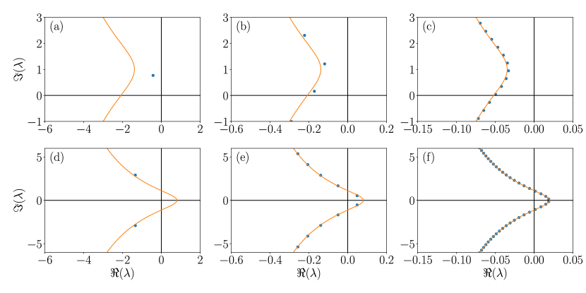
Figure 4.1. Spectrum (blue points) and the asymptotic continuous spectrum (4.7) (orange lines) of the scalar system (4.10). The upper panels (a-c) correspond to an absolutely stable case for the parameter values $a_{0}=-1+i$ and $a_{1}=0.5$. Time-delay is increasing from (a) to (c): $\tau=0.5$ (a), $\tau=5$ (b), and $\tau=20$ (c). Similarly, the lower panels (d-f) illustrate a case without absolute stability for the parameter values $a_{0}=-1$ and $a_{1}=-1.5$. Time-delays are: $\tau=0.5$ (d); $\tau=5$ (e), and $\tau=20$ (f).

4.5. Discussion of Corollary 6

Here we explain the physical meaning of the extended singular map (2.4), which appears in Corollary 6 and determines the absolute stability. According to the corollary assumptions, it must be exponentially stable for all $\omega\neq 0$ and any $\varphi\in\mathbb{T}$. The map (2.4) can be obtained form the single-delay DDE by substituting $x(t)=y(t)e^{i\omega t/\varepsilon}$, $\varphi=$$\omega/\varepsilon$, and formally neglecting the term $\varepsilon\dot{y}$. From the physical point of view, equation (2.4) regulates the amplification or damping of rapid oscillations with frequency $\omega/\varepsilon$. By rescaling the time back to the original form, these are frequencies $\omega$.

5. Multiple delays

5.1. Equivalence of absolute stability and asymptotic stability for hierarchically large delays

In this section we show that the criterium for the absolute stability for arbitrary positive delays is equivalent to the stability for hierarchically large time-delays, i.e., the asymptotic stability for $1\ll\tau_{1}\ll\cdots\ll\tau_{m}$. Such an equivalence is a generalization of Corollary 4 for one large delay. Interestingly, due to the symmetry of the conditions for the absolute stability with respect to the numbering of the delays, the order $\tau_{k}$ in this case does not play any role.

For the proof, we will need several Lemmas.

Lemma 14.

Let $A\in\mathbb{C}^{n\times n}$ and $i\omega_{0}\in\sigma(A)$. Then, for any $B\in\mathbb{C}^{n\times n}$, one of the following two mutually exclusive cases occurs:
I. There exist $\tilde{\omega}\neq 0$ and $\tilde{\varphi}\in\mathbb{T}$ such that $i\tilde{\omega}\in\sigma\left(A+Be^{i\tilde{\varphi}}\right)$.
II. $\omega_{0}=0$ and $0\in\sigma\left(A+Be^{i\varphi}\right)$ for all $\varphi\in\mathbb{T}$.

Proof.

Consider the function

$$Q(i\omega,z)=\det\left(-i\omega\text{I}+A+zB\right).$$

The Lemma’s assumption implies $Q(i\omega_{0},0)=0$. Two cases are possible:
1. The polynomial $Q(i\omega_{0},z)$ does not depend on $z$. In such a case, for arbitrary $z$, we have $Q(i\omega_{0},z)=Q(i\omega_{0},0)=0$. In particular, it holds $Q(i\omega_{0},e^{i\varphi})=0$, hence, $i\omega_{0}\in\sigma\left(A+Be^{i\varphi}\right)$ for all $\varphi$. If $\omega_{0}=0$, then the case II is realized. For $\omega_{0}\neq 0$, the case I is realized.
2) The polynomial $Q(i\omega_{0},z)$ depends non-trivially on $z$. Then, there exists a branch of complex roots $z(\omega)$ solving $Q(i\omega,z(\omega))=0$, which depends continuously on $\omega$, and $z(\omega_{0})=0$. Moreover, it holds $\left|z(\omega)\right|\to\infty$ as $\left|\omega\right|\to\infty$. Due to continuity, there exist $\tilde{\omega}_{1}\in(\omega_{0},\infty)$ and $\tilde{\omega}_{2}\in(-\infty,\omega_{0})$ such that $\left|z(\tilde{\omega}_{1,2})\right|=1.$ Hence, we obtain $i\tilde{\omega}_{1,2}\in\sigma\left(A+Be^{i\tilde{\varphi}_{1,2}}\right)$ with $\tilde{\varphi}_{1,2}=\arg(z(\tilde{\omega}_{1,2}))$. Since the two values $\tilde{\omega}_{1,2}$ cannot be zero simultaneously, we obtain the case I of the Lemma. ∎

Lemma 15.

Let $A_{0}\in\mathbb{C}^{n\times n}$ be Hurwitz and $A_{k}\in\mathbb{C}^{n\times n}$, $k=1,\dots,m$. Then, one of the following three mutually exclusive cases occurs:
I. $S(\text{$\Phi$})$ is Hurwitz for all $\Phi\in\mathbb{T}^{m}$;
II. There exist $\tilde{\omega}\neq 0$ and $\tilde{\Phi}\in\mathbb{T}^{m}$ such that $i\tilde{\omega}\in\sigma\left(S(\tilde{\text{$\Phi$}})\right)$;
III. There exists a nonempty set $\mathcal{T}_{0}\subset\mathbb{T}^{m}$, $\mathcal{T}_{0}\neq\mathbb{T}^{m}$, such that $0\in\sigma\left(S(\text{$\Phi$})\right)$ for $\Phi\in\mathcal{T}_{0}$, and $S(\text{$\Phi$})$ is Hurwitz for all $\Phi\in\mathbb{T}^{m}\setminus\mathcal{T}_{0}$.

Proof.

The proof follows from the consecutive application Lemmas 9 and 14 to the matrices

(5.1) $$M_{r}=A_{0}+\sum_{k=1}^{r}A_{k}e^{i\phi_{k}},r=0,...,m,$$

where $M_{r-1}$, $r=1,..,m$, plays the role of $A$ and $A_{r}$ plays the role of $B$. Note that in this way Case I of Lemma 9 transfers the Hurwitz property to the next level $r$, while Case II of Lemma 9 provides a resonance, which is then by Lemma 14 transfers to the next level. Case III of Lemma 9 detects a zero eigenvalue, which is transferred by Case II of Lemma 14. By considering all possible logical chains, wee see that I-III are the only possibilities that can be realized.

• Case I of Lemma 9 for all $r=1,\dots,m$. In this case, all matrices are Hurwitz for all $\Phi$.

• Case I of Lemma 9, followed by Case II of Lemma 9, possibly followed by Case I of Lemma 14. Here, we have $i\omega\in\sigma\left(M_{r}\right)$ for some $r\leq m$, $\omega\neq 0$. Then the sequential application of Lemma 14 $m-r$ times leads to $i\tilde{\omega}\in\sigma(S(\tilde{\Phi}))$ with $\tilde{\omega}\neq 0$ and some $\tilde{\Phi}$.

• Case I of Lemma 9, followed by Case III of Lemma 9, followed by Case I of Lemma 14. Here, the matrix $M_{r}$ contains zero eigenvalue for some $\Phi$ and otherwise it is Hurwitz for all other $\Phi$. At some further application of Lemma 14 on some level $r_{1}>r$, there appears a resonance $\omega\neq 0$ such that $i\omega\in\sigma\left(A_{0}+\sum_{k=1}^{r_{1}}A_{k}e^{i\tilde{\varphi_{k}}}\right)$, $r<r_{1}\leq m$. Further application of Lemma 14 $m-r_{1}$ times leads to the statement II of this Lemma.

• Case I of Lemma 9, followed by Case III of Lemma 9, followed by Case II of Lemma 14. Similarly to the previous case, some matrix $M_{r}$ contains zero eigenvalue and otherwise it is Hurwitz for all other $\Phi$. At some further applications of Lemma 14, only case II of Lemma 14 is realized. We must only show that $\mathcal{T}_{0}\neq\mathbb{T}^{m}$. Indeed, assuming opposite, we have $0\in S(\Phi)$ for all $\Phi$, which implies $0\in A_{0}$ and contradicts the assumption of $A_{0}$ Hurwitz.

• Case I of Lemma 9, followed by Case III of Lemma 9, followed by Case II of Lemma 14, followed by Case I of Lemma 14. This logical chain is similar to the previous one, with only difference that the case I of Lemma 14 is realized at some later iteration.

∎

Lemma 16.

Let $A_{k}\in\mathbb{C}^{n\times n}$, $k=1,\dots,m$, and $i\omega_{0}\in\sigma(A_{0})$. Then, one of the following two mutually exclusive cases occurs:
I. There exist $\tilde{\omega}\neq 0$ and $\tilde{\Phi}$ such that $i\tilde{\omega}\in\sigma(S(\tilde{\Phi}))$;
II. $\omega_{0}=0$ and $0\in\sigma(S(\text{$\Phi$}))$ for all $\Phi\in\mathbb{T}^{m}$.

Proof.

The proof follows from the sequential application of Lemma 14 in a similar way as above. ∎

Lemma 17 (Reappearance of resonances).

Let $A_{k}\in\mathbb{C}^{n\times n}$, $k=0,\dots,m$, and $i\omega_{0}\in\sigma(S(\Phi))$, $\omega_{0}\neq 0$. Then, it holds

(5.2) $$\det\left[-i\omega_{0}\text{I}+A_{0}+\sum_{k=1}^{m}A_{k}e^{-i\omega_{0}\tau_{k}}\right]=0$$

with

(5.3) $$\tau_{k}=\frac{2\pi}{\omega_{0}}n_{k}-\frac{\varphi_{k}}{\omega_{0}},\quad n_{k}\in\mathbb{Z}.$$

That is, $i\omega_{0}$ solves the characteristic equation (1.2) for countably many time-delays (5.3).
In particular, among these time-delays, one can choose the set $\left\{\tau_{1},\dots,\tau_{m}\right\}$ of hierarchically large delays, which satisfy the condition (2.1) with arbitrary small $\varepsilon>0$. Such delays are hierarchically ordered so that $\tau_{k}/\tau_{k+1}=\varepsilon(\nu_{k}/\nu_{k+1})$.

Proof.

The fact that Eq. (5.2) holds for time-delays (5.3) can be checked by substitution.

Let us show that time delays can be chosen to be hierarchical, i.e., satisfy the condition (2.1) with arbitrary small $\varepsilon>0$. We denote

$$\varepsilon=\frac{1}{\tau_{1}}=\frac{\omega_{0}}{2\pi n_{1}-\varphi_{1}},$$

which is a small parameter for sufficiently large $n_{1}$. We assume, in particular, that $n_{1}\gg\omega_{0}$. Such a definition of $\varepsilon$ implies equality (2.1) for $k=1$.

Let us show that $n_{k}$, and, hence $\tau_{k}$, can be chosen in such a way that (2.1) holds for some $\nu_{k}\in[1,1+\varepsilon^{k-1})$. The equality

$$\tau_{k}=\frac{2\pi n_{k}-\varphi_{k}}{\omega_{0}}=\nu_{k}\varepsilon^{-k}$$

leads to

(5.4) $$n_{k}=\frac{\varphi_{k}}{2\pi}+\frac{\omega_{0}\nu_{k}}{2\pi\varepsilon^{k}}.$$

By increasing $\nu_{k}$ from 1 to $1+\frac{2\pi\varepsilon^{k}}{\left|\omega_{0}\right|}$, the value of $n_{k}$ in Eq. (5.4) changes by 1. Hence, there exists such $\nu_{k}\in[1,1+\frac{2\pi\varepsilon^{k}}{\left|\omega_{0}\right|})$ that $n_{k}$ admits an integer value. Finally, by choosing $\varepsilon$ sufficiently small such that $\frac{2\pi\varepsilon}{\left|\omega_{0}\right|}<1$, we obtain that $\nu_{k}\in[1,1+\varepsilon^{k-1})$. ∎

We remark that Lemma (17) generalizes some of the statements shown for one delay in [71].

Proof of Theorem 5.

It is clear that the absolute stability implies the stability for hierarchically large time delays. Therefore, it remains to show that conditions (A1.1) [instantaneous stability], (A1.2) [nonsingular $S(0)$], and (A1.3) [no resonance] of Theorem 2 are necessary for the stability of the systems with hierarchically large time delays (2.1).

1. First, we show that (A1.1) [instantaneous stability] is necessary. Assume the opposite, i.e., the condition (A1.1) of Theorem 2 does not hold. Then either $i\omega_{0}\in\sigma\left(A_{0}\right)$ or $\lambda_{0}\in\sigma\left(A_{0}\right)$ with $\Re(\lambda_{0})>0$.

1a: Consider the case $i\omega_{0}\in\sigma\left(A_{0}\right)$. Then, Lemma 16 implies that one of the two cases can occur:

1aa: $i\tilde{\omega}\in\sigma(S(\tilde{\Phi}))$ with some $\tilde{\omega}\neq 0$. In such a case, Lemma 17 implies that $i\tilde{\omega}$ is a solution of the characteristic equation for hierarchically large time delays (2.1). We obtain the contradiction to the absolute stability and, hence, (A1.1) holds.

1ab: $\omega_{0}=0$ and $0\in\sigma(S(\Phi))$ for all $\Phi\in\mathbb{T}^{m}$. In particular, it holds $0\in\sigma(S(0))$, which means that $\lambda=0$ is an eigenvalue for arbitrary time-delays. This contradicts the absolute stability assumption for hierarchically large delays, hence, (A1.1) holds.

1b: Consider the case $\lambda_{0}\in\sigma\left(A_{0}\right)$ with $\Re(\lambda_{0})>0$. Let $\tau_{k}=\nu_{k}\varepsilon^{-k}$ be hierarchically large delays, and the corresponding characteristic equation

(5.5) $$P_{m}(\lambda)=\det\left[-\lambda\text{I}+A_{0}+\sum_{k=1}^{m}A_{k}e^{-\lambda\nu_{k}\varepsilon^{-k}}\right]=0.$$

Let $U(\lambda_{0})$ be a sufficiently small open neighborhood of $\lambda_{0}$ such that it does not contain other eigenvalues of $A_{0}$, and $\Re(U(\lambda_{0}))>0$. Then, the holomorphic function $P_{m}(\lambda)$ converges uniformly to $\det\left[-\lambda\text{I}+A_{0}\right]$ for $\varepsilon\to 0$. According to the Hurwitz theorem, the characteristic equation (5.5) has an unstable root in $\lambda\in U(\lambda_{0})$ for all sufficiently small $\varepsilon$. This contradicts the asymptotic stability assumption for hierarchically large delays, and, hence, (A1.1) holds.

2. We show that (A1.2) [nonsingular $S(0)$] is necessary. Assume that the condition (A1.2) of Theorem 2 does not hold. Then $0\in\sigma(S(0))$ and, hence the characteristic root $\lambda=0$ solves Eq. (1.2) for all delays. This contradicts the asymptotic stability assumption for hierarchically large delays, and, hence, (A1.2) holds.

3. We show that (A1.3) [no resonance] is necessary for the stability of systems with hierarchically large time delays. Assume (A1.3) does not hold. Then there exists

$$i\omega_{0}\in\sigma\left(S(\Phi)\right),\quad\omega_{0}\neq 0.$$

Lemma 17 implies that there are hierarchically large time delays, for which there exists the eigenvalue $i\omega_{0}$. This contradicts the asymptotic stability assumption and, hence, (A1.3) holds. ∎

5.2. Asymptotic spectrum for multiple hierarchically large delays and its relation to the conditions for absolute stability

Let us briefly review some concepts for the spectrum of systems with hierarchically large time-delays $\tau_{k}=\nu_{k}\varepsilon^{-k}$ from [72]. This spectrum can be generically divided into $m+1$ parts corresponding to different timescales:

(i) The strongly unstable part $\mathcal{S}_{\text{su}}$, which is approximated by the unstable spectrum of $A_{0}$, i.e. $\sigma(A_{0})$ with $\Re\left(A_{0}\right)>0$.

(ii) The asymptotic continuous spectrum on different timescales can be described by the following sets

(5.6) $$B_{k,j}=\left\{z\in\mathbb{C}:-\ln\left|Y_{k,j}(\omega,\varphi_{1},\dots,\varphi_{k-1})\right|\varepsilon^{k}+i\omega,\,\,\omega\in\mathbb{R}\right\},$$

where $k=1,\dots,m$. The functions $Y_{k,j}(\omega,\varphi_{1},\dots,\varphi_{k-1})$ are the $j$-th roots of the spectral polynomial

(5.7) $$P_{k}(\omega,\varphi_{1},\dots,\varphi_{k-1},Y)=\det\left[i\omega\cdot\mathrm{I}-A_{0}-\sum_{l=1}^{k-1}A_{l}e^{i\varphi_{j}}-A_{k}Y\right],$$

where the index $j$ numbers the roots. The sets $B_{k,j}$ correspond to the eigenvalues with the real parts converging to zero as $\varepsilon^{k}$. For $m=1$, the the sets $B_{1,j}$ contain the asymptotic continuous spectrum of systems with one large delay $\tau_{1}$.

In the non-degenerate case of $\det A_{m}\neq 0$, the asymptotic spectrum has the form

$$\mathcal{S}_{\text{su}}\bigcup\Biggl{[}\bigcup_{\begin{subarray}{c}k=1,\dots,m-1\\ j=1,\dots,\text{rank}A_{k}\end{subarray}}B_{k,j}^{+}\Biggr{]}\bigcup\Biggl{[}\bigcup_{j=1}^{\text{rank}A_{m}}B_{m,j}\Biggr{]},$$

where $B_{k.j}^{+}=B_{k,j}\bigcap\left\{z:\,\Re z>0\right\}$. That is, for all spectral components that correspond to the convergence of real parts as $\mathcal{O}(\varepsilon^{k})$ with $k=1,\dots,m-1$, only the unstable part is included. The stable part of the asymptotic continuous spectrum can contain only $B_{m,j}$, which has the slowest convergence $\varepsilon^{m}$ of the real parts to zero. This implies that the destabilization of the system with hierarchical delays with $\det A_{m}\neq 0$ can occur only due to some $B_{m,j}$ spectral component, which is caused by the largest delay $\tau_{m}$. In a degenerate case of $\det A_{m}=0$, stable parts of other spectral components may appear as well, see more details in [59, 5, 7, 72].

Taking into account different part of the asymptotic spectra, we can interpret the role of the conditions of Theorems 2 and 3 for the spectrum of systems with hierarchical time delays. Condition (A1.1) [instantaneous stability] guarantees the absence of the strongly unstable spectrum. Condition (A1.2) [nonsingular $S(0)$] guarantees the absence of the zero eigenvalue. Conditions (A1.3) [no resonance] and (A2.2) [almost Hurwitz S($\Phi$)] guarantee that the asymptotic continuous spectrum is stable and do not cross the imaginary axis.

5.3. Illustration in the case of two delays

Figure 5.1 illustrates the spectrum of the scalar DDE with two delays

(5.8) $$\dot{x}(t)=a_{0}x(t)+a_{1}x(t-\tau_{1})+a_{2}x(t-\tau_{2}).$$

In particular, Figs. 5.1(a)-(c) show an absolutely stable case for different values of time-delays. With the increasing of the delays, the spectrum fills certain regions of the complex plane but stays stable. Figs. 5.1(d)-(f) illustrate the case without absolute stability. One can observes a stability for small delays and destabilization with the increasing of the delays.

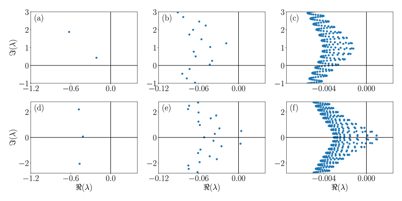
Figure 5.1. Spectrum (blue points) of the scalar system (5.8) with two delays. The upper panel (a-c) corresponds to an absolutely stable case for the parameter values $a_{0}=-1+i$, $a_{1}=0.5$, and $a_{2}=0.3$. Time-delay is increasing from (a) to (c): $\tau_{1}=0.5$, $\tau_{2}=2.5$ (a), $\tau_{1}=5$, $\tau_{2}=25$ (b), and $\tau_{1}=20$, $\tau_{2}=400$ (c). The lower panel (d-f) illustrates the case without absolute stability for $a_{0}=-1$, $a_{1}=-0.7$, and $a_{2}=0.5+0.1i$. Time-delays are: $\tau_{1}=0.5$, $\tau_{2}=2.5$ (d), $\tau_{1}=5$, $\tau_{2}=25$ (e), and $\tau_{1}=20$, $\tau_{2}=400$ (f).

6. Proof of Theorems 2 and 3

Lemma 18.

Let $A\in\mathbb{C}^{n\times n}$ be not Hurwitz and $0\not\in\sigma(A)$. Then, for any $B\in\mathbb{C}^{n\times n}$ , there exists $\varphi\in\mathbb{T}$ such that the matrix $A+Be^{i\varphi}$ is not Hurwitz and $\lambda\in\sigma(A+Be^{i\varphi})$ with $\lambda\neq 0$ and $\Re(\lambda)\geq 0$.

Proof.

1. Consider first the case $i\omega_{0}\in\sigma(A)$, $\omega_{0}\neq 0$. Then Lemma 14 implies that $i\tilde{\omega}\in A+Be^{i\tilde{\varphi}}$, $\tilde{\omega}\neq 0$ for some $\tilde{\varphi}$. Thus, the statement of the Lemma follows with $\lambda=i\tilde{\omega}$ and $\varphi=\tilde{\varphi}$.

2. Let $\lambda\in\sigma(A)$ with $\Re(\lambda)>0$. The following proof uses similar ideas as in the proof of Lemma 9. Consider the function

$$Q(\lambda,z)=\det\left(-\lambda\text{I}+A+zB\right).$$

As a polynomial in $\lambda$, it possesses a continuous branch of roots $\lambda(z)$ such that $\Re(\lambda(0))>0$. Due to continuity of $\lambda(z)$, two cases are possible:

2a. $\Re(\lambda(z))>0$ for all $z$ with $\left|z\right|\leq 1$. In this case, taking $z=e^{i\varphi}$, we obtain that $A+Be^{i\varphi}$ contains an eigenvalue with $\Re(\lambda(z))>0$ for all $\varphi$.

2b. There exists $\hat{z}$ such that $\lambda(\hat{z})=i\hat{\omega}$ and $\Re\left(\lambda(z)\right)>0$ for all $|z|<|\hat{z}|$. That is, we obtain

(6.1) $$Q(i\hat{\omega},\hat{z}) =\det\left(-i\hat{\omega}\text{I}+A+\hat{z}B\right)=0,\quad\left|\hat{z}\right|\leq 1,$$

(6.2) $$\Re\left(\lambda(z)\right)>0\,\,\,\text{for\,\,all}\,\,|z|<|\hat{z}|.$$

2b-i. Consider the case $|\hat{z}|=1$. We denote $\hat{z}=e^{i\hat{\varphi}}$. If $\hat{\omega}\neq 0$, we obtain $i\hat{\omega}\in A+Be^{i\hat{\varphi}}$, which is needed for the proof. If $\hat{\omega}\neq 0$, we observe that $\Re\left(\lambda(z)\right)\geq 0$ for all $z=e^{i\varphi}$. Moreover, the equality $\lambda(e^{i\varphi})=0$ cannot hold for all $\varphi$, since, otherwise, $0\in\sigma\left(A+Be^{i\varphi}\right)$ for all $\varphi$, which is only possible for $0\in\sigma(A)$. Therefore, there exists $\tilde{\varphi}$ such that $\lambda\in\sigma\left(A+Be^{i\tilde{\varphi}}\right)$ with $\lambda\neq 0$ and $\Re(\lambda)\geq 0$.

2b-ii. In the case $\left|\hat{z}\right|<1$, consider the function

$$Q(i\omega,z)=\det\left(-i\omega\text{I}+A+zB\right)$$

as a polynomial in $z$. It is nontrivial in $z$ at $\omega=\hat{\omega}$ and $z=\hat{z}$, and there exists a continuous branch of roots such that $z(\hat{\omega})=\hat{z}$, $\left|\hat{z}\right|<1$, and $\left|z(\omega)\right|\to\infty$ as $\left|\omega\right|\to\infty$. By continuity, we obtain the existence of $\tilde{\omega}_{1,2}$ with $z(\tilde{\omega}_{1,2})=e^{i\tilde{\varphi}_{1,2}}$. Hence, we have $i\tilde{\omega}_{1,2}\in\sigma\left(A+Be^{i\tilde{\varphi}_{1,2}}\right)$. Since $\tilde{\omega}_{1}$ and $\tilde{\omega_{2}}$ belong to disjoint intervals $(-\infty,\hat{\omega})$ and $(\hat{\omega},+\infty)$, at least one of them is nonzero. ∎

Proof of Theorems 2 and 3..

Firstly, we show that the conditions of Theorems 2 and 3 are equivalent.

1. The conditions (A2.2) [almost Hurwitz S($\Phi$)] and (A1.2) [nonsingular $S(0)$] imply that $A_{0}$ is Hurwitz, i.e., (A1.1) [instantaneous stability] holds. Assume the opposite, i.e., $A_{0}$ is not Hurwitz.

When $i\omega_{0}\in\sigma(A_{0}),$ Lemma 16 implies that one of the following two cases occur:

I. There exists $\omega\neq 0$ such that $i\omega\in\sigma(S(\Phi))$ for some $\Phi$. This contradicts the condition (A2.2) [almost Hurwitz S($\Phi$)].

II. $\omega_{0}=0$ and $0\in\sigma(S(\Phi))$ for all $\Phi\in\mathbb{T}^{m}$. Substituting $\Phi=0$, we obtain $0\in\sigma(S(0))$, which contradicts the condition (A1.2) [nonsingular $S(0)$].

Now assume that $\sigma(A_{0})$ does not contain purely imaginary eigenvalues. Since $A_{0}$ is not Hurwitz, we have $\lambda\in\sigma(A)$ with $\Re(\lambda)>0$. Applying Lemma (18) sequentially, we obtain that there is $\lambda\in\sigma(S(\Phi))$ with some $\Phi$ with $\Re(\lambda)\geq 0$ and $\lambda\neq 0$. This contradicts to the condition (A2.2) [almost Hurwitz S($\Phi$)].

We have shown that $A_{0}$ is Hurwitz under the assumptions of Theorem 3. Let us show that (A2.2) [almost Hurwitz S($\Phi$)] and (A1.3) [no resonance] are equivalent when $A_{0}$ is Hurwitz. Applying Lemma 15, one can see that cases I and III of Lemma 15 correspond to the condition (A2.2) [almost Hurwitz S($\Phi$)] of Theorem 3. Moreover, the condition (A1.3) [no resonance] of Theorem 2 excludes the case II of Lemma 15, hence, it is also equivalent to the case I or III of Lemma 15. Hence, (A1.3) and (A2.2) are equivalent.

The following steps (ii)–(iii) prove that (A1.2) [nonsingular $S(0)$] and (A2.2) [almost Hurwitz S($\Phi$)] are sufficient for the absolute stability.

2. First notice, that (A2.2) [almost Hurwitz S($\Phi$)] implies that $S(0)$ is almost Hurwitz, i.e., $S(0)$ is Hurwitz, except for a possible zero eigenvalue. However, zero eigenvalue is excluded by the condition (A1.2) [nonsingular $S(0)$]. Hence, $S(0)$ is Hurwitz.

The spectrum for $\tau_{k}=0$, $k=1,\dots,m$ coincides with the spectrum of $S(0)$, which is Hurwitz. Hence, all roots for $\tau_{k}=0$ possess negative real parts. The same also holds for sufficiently small delays, see e.g. [12].

3. Due to continuity of the roots $\lambda$ with respect to $\tau_{k}>0$, the only possible stability loss for positive delays is through the crossing of the imaginary axis. Let us assume that $\lambda=i\omega^{*}$ at some $\tau_{k}=\tau_{k}^{*}>0$, $k=1,\dots,m$, and subsequently show that it leads to a contradiction. Indeed $\lambda=i\omega^{*}$ implies

$$i\omega^{*}\in\sigma\left(S(\Phi^{*})\right),\quad\varphi_{k}^{*}=-\omega^{*}\tau_{k}^{*}.$$

Due to (A2.2) [almost Hurwitz S($\Phi$)], it holds $\omega^{*}=0$. However, in this case, $0\in\sigma\left(S(0)\right)$, which contradicts the assumption (A1.2) [nonsingular $S(0)$].

Hence, for all positive delays, the roots cannot cross the imaginary axis and the asymptotic stability holds, i.e. the conditions (A1.2) and (A2.2) imply the absolute stability.

The following steps (iv)-(vi) prove that (A1.1) [instantaneous stability], (A1.2) [nonsingular $S(0)$], and (A1.3) [no resonance] are necessary conditions for the absolute stability. We choose here the conditions (A1.1), (A1.2), (A1.3) from Theorem 2, since they are equivalent to (A1.2) and (A2.2), and they are more convenient for the proof of necessity. Hence, we assume that absolute stability holds and show (A1.1), (A1.2), and (A1.3).

(iv) Assume (A1.1) [instantaneous stability] does not hold, then there exists $\lambda_{0}\in\sigma(A_{0})$ with $\Re\left(\lambda_{0}\right)\geq 0$.

If $\Re\left(\lambda_{0}\right)>0$, consider the case of large delays $\tau_{k}=\varepsilon^{-1}$. The corresponding characteristic equation has the form

(6.3) $$P_{m}(\lambda)=\det\left[-\lambda\text{I}+A_{0}+\sum_{k=1}^{m}A_{k}e^{-\lambda/\varepsilon}\right]=0.$$

Let $U(\lambda_{0})\subset\mathbb{C}$ be a sufficiently small open neighborhood of $\lambda_{0}$ such that it does not contain other eigenvalues of $A_{0}$, and $\Re(U(\lambda_{0}))>0$. Then, the holomorphic function $P_{m}(\lambda)$ converges uniformly to $\det\left[-\lambda\text{I}+A_{0}\right]$ for $\varepsilon\to 0$ on $U(\lambda_{0})$. According to the Hurwitz theorem, the characteristic equation (6.3) has an unstable root in $\lambda\in U(\lambda_{0})$ for all sufficiently small $\varepsilon$. This contradicts to the absolute stability assumption and, hence, (A1.1) is a necessary condition.

If $i\omega_{0}\in\sigma\left(A_{0}\right)$, Lemma 16 implies that one of the two cases can occur:

1. $i\tilde{\omega}\in\sigma\left(S(\tilde{\Phi})\right)$ with some $\tilde{\omega}\neq 0$. In such a case, Lemma 17 implies that $i\tilde{\omega}$ is a solution of the characteristic equation for countable number of delays (5.3). We obtain the contradiction to the absolute stability and, hence, (A1.1) is necessary.

2. $\omega_{0}=0$ and $0\in\sigma\left(S(\Phi)\right)$ for all $\Phi\in\mathbb{T}^{m}$. In particular, it holds $0\in\sigma\left(S(0)\right)$, which means that $\lambda=0$ is an eigenvalue for arbitrary time-delays. This contradicts the absolute stability assumption, hence, (A1.1) is necessary.

(v) The necessity of (A1.2) [nonsingular $S(0)$] is evident, since otherwise there exists a root $\lambda=0$ for all delays.

(vi) We show that (A1.3) [no resonance] is necessary. Assume the opposite, i.e., $i\omega_{0}\in\sigma(S(\Phi))$, $\omega_{0}\neq 0$ for some $\Phi$. Then, accordingly to Lemma 17, systems with time-delays (5.3) possess the eigenvalues $i\omega_{0}$. This contradicts the absolute stability and proves that (A1.3) is necessary.

Finally, let us show the criterion for the absolute hyperbolicity from Theorem 2. We first prove that (A1.2) [nonsingular $S(0)$] and (A1.3) [no resonance] imply absolute hyperbolicity. Assume the opposite, so that there exists a solution $\lambda=i\omega$ of Eq. (1.2) for some time delays. Then, if $\omega=0$, then we obtain the contradiction to (A1.2); if $\omega\neq 0$, we obtain the contradiction to (A1.3) with $\varphi_{k}=-\omega\tau_{k}$. The backward statement “absolute hyperbolicity” $\Rightarrow$ (A1.2) and (A1.3) is also straightforward. Assuming that (A1.2) or (A1.3) does not hold, we obtain either $\lambda=0$ or $\lambda=i\omega\neq 0$, respectively. ∎

7. Conclusions

The obtained conditions for absolute stability determine a class of linear DDEs, which are asymptotically exponentially stable, independently on time-delays. Such class of systems can be useful for applications, where the robustness against time-delays is important. For nonlinear systems, these conditions exclude the possibility of any bifurcations at the corresponding equilibrium.

Bifurcations induced by varying time delay are also excluded in the case of absolute hyperbolicity. Linear systems that do not belong to one of these two classes have resonances, i.e. purely imaginary eigenvalues, which occur for countably many resonant delay times in each delayed argument, and are necessarily unstable for large delays. Note that such systems may or may not become stable for certain ranges of small delays. Even systems with strong instabilities for large delay may become stable for small delay, but only if they have unstable asymptotic continuous spectrum. This counter-intuitive conclusion follows from absolute hyperbolicity, which we showed for strongly unstable systems with stable asymptotic continuous spectrum.

Acknowledgment: SY was supported by the German Science Foundation (Deutsche Forschungsgemeinschaft, DFG) [project No. 11803875]. TP was supported by a Newton Advanced Fellowsip of the Royal Society NAF\R1\180236, by Serrapilheira Institute (Grant No. Serra-1709-16124), and FAPESP (grant 2013/07375-0).

References

- [1] Thomas Erneux. Applied Delay Differential Equations, volume 3 of Surveys and Tutorials in the Applied Mathematical Sciences. Springer, 2009.
- [2] Lionel Weicker, Thomas Erneux, Otti D’Huys, Jan Danckaert, Maxime Jacquot, Yanne Chembo, and Laurent Larger. Strongly asymmetric square waves in a time-delayed system. Physical Review E, 86(5):055201, nov 2012.
- [3] Miguel C. Soriano, Jordi García-Ojalvo, Claudio R. Mirasso, and Ingo Fischer. Complex photonics: Dynamics and applications of delay-coupled semiconductors lasers. Reviews of Modern Physics, 85(1):421–470, mar 2013.
- [4] A Glitzky, A Mielke, L Recke, M Wolfrum, and S Yanchuk. Mathematics of optoelectronic devices. In P Deuflhard Et al., editor, MATHEON - Mathematics for Key Technologies, volume 1 of EMS Series in Industrial and Applied Mathematics, pages 243–256. EMS, 2014.
- [5] Serhiy Yanchuk and Giovanni Giacomelli. Pattern formation in systems with multiple delayed feedbacks. Physical Review Letters, 112(17):1–5, may 2014.
- [6] Thomas Erneux, Julien Javaloyes, Matthias Wolfrum, and Serhiy Yanchuk. Introduction to Focus Issue: Time-delay dynamics. Chaos: An Interdisciplinary Journal of Nonlinear Science, 27(11):114201, nov 2017.
- [7] Serhiy Yanchuk and Giovanni Giacomelli. Spatio-temporal phenomena in complex systems with time delays. Journal of Physics A: Mathematical and Theoretical, 50(10):103001, mar 2017.
- [8] Yang Kuang. Delay differential equations with applications in population dynamics, volume 35 of Mathematics in science and engineering. Academic Press, 1993.
- [9] Hal L. Smith. Reduction of structured population models to threshold-type delay equations and functional differential equations: a case study. Mathematical Biosciences, 113(1):1–23, jan 1993.
- [10] Ferenc Hartung, Tibor Krisztin, Hans Otto Walther, and Jianhong Wu. Chapter 5 Functional Differential Equations with State-Dependent Delays: Theory and Applications. Handbook of Differential Equations: Ordinary Differential Equations, 2006.
- [11] Odo Diekmann and Mats Gyllenberg. Abstract Delay Equations Inspired by Population Dynamics. In Functional Analysis and Evolution Equations, pages 187–200. Birkhäuser Basel, Basel, 2007.
- [12] Hal L Smith. An Introduction to Delay Differential Equations with Applications to the Life Sciences, volume 57 of Texts in Applied Mathematics. Springer Science+ Business Media, New York, NY, 2010.
- [13] Johannes Müller and Christina Kuttler. Methods and Models in Mathematical Biology. Lecture Notes on Mathematical Modelling in the Life Sciences. Springer Berlin Heidelberg, Berlin, Heidelberg, 2015.
- [14] G.O. Agaba, Y.N. Kyrychko, and K.B. Blyuss. Dynamics of vaccination in a time-delayed epidemic model with awareness. Mathematical Biosciences, 294:92–99, dec 2017.
- [15] Lai Sang Young, Stefan Ruschel, Serhiy Yanchuk, and Tiago Pereira. Consequences of delays and imperfect implementation of isolation in epidemic control. Scientific Reports, 9(1):3505, dec 2019.
- [16] Stefan Ruschel, Tiago Pereira, Serhiy Yanchuk, and Lai-Sang Young. An SIQ delay differential equations model for disease control via isolation. Journal of Mathematical Biology, 79(1):249–279, jul 2019.
- [17] Jianhong Wu. Introduction to Neural Dynamics and signal Transmission Delay, volume 6. Walter de Gruyter, 2001.
- [18] Eugene M. Izhikevich. Polychronization: Computation with Spikes. Neural Computation, 18(2):245–282, feb 2006.
- [19] Tae-Wook Ko and G Bard Ermentrout. Effects of axonal time delay on synchronization and wave formation in sparsely coupled neuronal oscillators. Physical Review E (Statistical, Nonlinear, and Soft Matter Physics), 76(5):56206, 2007.
- [20] Oleksandr V. Popovych, Serhiy Yanchuk, and Peter A. Tass. Delay- and Coupling-Induced Firing Patterns in Oscillatory Neural Loops. Physical Review Letters, 107(22):228102, nov 2011.
- [21] Serhiy Yanchuk, Stefan Ruschel, Jan Sieber, and Matthias Wolfrum. Temporal Dissipative Solitons in Time-Delay Feedback Systems. Physical Review Letters, 123(5):053901, jul 2019.
- [22] L Appeltant, M.C. C Soriano, G Van der Sande, J Danckaert, S Massar, J Dambre, B Schrauwen, C.R. R Mirasso, and I Fischer. Information processing using a single dynamical node as complex system. Nature Communications, 2(1):468, sep 2011.
- [23] L Larger, M C Soriano, D Brunner, L Appeltant, J M Gutierrez, L Pesquera, C R Mirasso, and I Fischer. Photonic information processing beyond Turing: an optoelectronic implementation of reservoir computing. Opt. Express, 20(3):3241–3249, jan 2012.
- [24] Laurent Larger, Antonio Baylón-Fuentes, Romain Martinenghi, Vladimir S. Udaltsov, Yanne K. Chembo, and Maxime Jacquot. High-speed photonic reservoir computing using a time-delay-based architecture: Million words per second classification. Physical Review X, 7(1):1–14, feb 2017.
- [25] Florian Stelzer, André Röhm, Kathy Lüdge, and Serhiy Yanchuk. Performance boost of time-delay reservoir computing by non-resonant clock cycle. Neural Networks, 124:158–169, apr 2020.
- [26] Mirko Goldmann, Felix Köster, Kathy Lüdge, and Serhiy Yanchuk. Deep time-delay reservoir computing: Dynamics and memory capacity. Chaos: An Interdisciplinary Journal of Nonlinear Science, 30(9):93124, sep 2020.
- [27] Tsu-Chin Tsao, Mark W. McCarthy, and Shiv G. Kapoor. A new approach to stability analysis of variable speed machining systems. International Journal of Machine Tools and Manufacture, 33(6):791–808, dec 1993.
- [28] Tamás Insperger, Gábor Stépán, and Janos Turi. State-dependent delay in regenerative turning processes. Nonlinear Dynamics, 47(1-3):275–283, dec 2006.
- [29] T Insperger and G Stépán. Semi-discretization for time-delay systems - Engineering applications. Springer, 2011.
- [30] Andreas Otto and Günter Radons. Application of spindle speed variation for chatter suppression in turning. CIRP Journal of Manufacturing Science and Technology, 6(2):102–109, jan 2013.
- [31] Andreas Otto and Günter Radons. The influence of tangential and torsional vibrations on the stability lobes in metal cutting. Nonlinear Dynamics, 82(4):1989–2000, dec 2015.
- [32] L. S. Pontryagin. On the zeros of some elementary transcendental functions. Izv. Akad. Nauk SSSR, Ser. Mat., 6:115–134, 1942.
- [33] A.D. Myshkis. General theory of differential equations with retarded arguments. Uspekhi Mat. Nauk, 4(5(33)):99–141, 1949.
- [34] Richard Ernest Bellman and John M. Danskin. A Survey of the Mathematical Theory of Time-Lag, Retarded Control, and Hereditary Processes. RAND Corporation, Santa Monica, CA, 1954.
- [35] Richard E Bellman and Kenneth L Cooke. Differential-Difference Equations. 6:462, 1963.
- [36] G. Stepan. Retarded dynamical systems : stability and characteristic functions. Longman Scientific & Technical, 1989.
- [37] Jack K. Hale and Sjoerd M. Verduyn Lunel. Introduction to Functional Differential Equations, volume 99. Springer-Verlag, 1993.
- [38] Odo Diekmann, Sjoerd M. Verduyn Lunel, Stephan A. van Gils, and Hanns-Otto Walther. Delay Equations, volume 110 of Applied Mathematical Sciences. Springer New York, New York, NY, 1995.
- [39] Fatihcan M Atay, editor. Complex Time-Delay Systems. Understanding Complex Systems. Springer Berlin Heidelberg, Berlin, Heidelberg, 2010.
- [40] Shangjiang Guo and Jianhong Wu. Bifurcation Theory of Functional Differential Equations, volume 184 of Applied Mathematical Sciences. Springer-Verlag New York, 2013.
- [41] Chin Yuang-Shun. Unconditional stability of systems with time-lags. Acta Mathematica Sinica, English Series, 1:125–142, 1960.
- [42] L Elsgolz and S. Norkin. Introduction to the theory of differential equations with retarded argument. Nauka, Moscow, 1971.
- [43] K L Cooke and P Van Den Driessche. On zeros of some transcendental functions. Funkcial. Ekvac., 29:77–90, 1986.
- [44] Fred Brauer. Absolute stability in delay equations. Journal of Differential Equations, 69(2):185–191, sep 1987.
- [45] Shigui Ruan and Junjie Wei. On the zeros of transcendental functions with applications to stability of delay differential equations with two delays. Dynamics of Continuous, Discrete and Impulsive Systems Series A, 10:863–874, 2003.
- [46] N. D. Hayes. Roots of the Transcendental Equation Associated with a Certain Difference-Differential Equation. Journal of the London Mathematical Society, s1-25(3):226–232, jul 1950.
- [47] V. W. Noonburg. Roots of a Transcendental Equation Associated with a System of Differential-Difference Equations. SIAM Journal on Applied Mathematics, 17(1):198–205, jan 1969.
- [48] F. G. Boese. Stability Criteria for Second-Order Dynamical Systems Involving Several Time Delays. SIAM Journal on Mathematical Analysis, 26(5):1306–1330, 1995.
- [49] Margarete Baptistini and Plácido Táboas. On the Stability of Some Exponential Polynomials. Journal of Mathematical Analysis and Applications, 205(1):259–272, jan 1997.
- [50] F.G Boese. Stability with Respect to the Delay: On a Paper of K. L. Cooke and P. van den Driessche. Journal of Mathematical Analysis and Applications, 228(2):293–321, dec 1998.
- [51] Vladimir B. Kolmanovskii. On the Liapunov-Krasovskii functionals for stability analysis of linear delay systems. International Journal of Control, 72(4):374–384, jan 1999.
- [52] Zidong Wang, Biao Huang, and H. Unbehauen. Robust reliable control for a class of uncertain nonlinear state-delayed systems. Automatica, 35(5):955–963, may 1999.
- [53] Fen Wu and Karolos M. Grigoriadis. LPV systems with parameter-varying time delays: Analysis and control. Automatica, 37(2):221–229, feb 2001.
- [54] Xianwei Li, Huijun Gao, and Keqin Gu. Delay-independent stability analysis of linear time-delay systems based on frequency discretization. Automatica, 70:288–294, aug 2016.
- [55] Qi An, Edoardo Beretta, Yang Kuang, Chuncheng Wang, and Hao Wang. Geometric stability switch criteria in delay differential equations with two delays and delay dependent parameters. Journal of Differential Equations, 266(11):7073–7100, may 2019.
- [56] Jack K Hale. Theory of Functional Differential Equations, volume 3 of Applied Mathematical Sciences. Springer-Verlag, 1977.
- [57] F. G. Boese. Delay-independent stability of a special sequence of neutral difference-differential equations with one delay. Journal of Differential Equations, 1991.
- [58] Jie Chen, Demin Xu, and Bahram Shafai. On Sufficient Conditions for Stability Independent of Delay. IEEE Transactions on Automatic Control, 40(9):1675–1680, 1995.
- [59] M. Lichtner, M. Wolfrum, and S. Yanchuk. The Spectrum of Delay Differential Equations with Large Delay. SIAM Journal on Mathematical Analysis, 43(2):788–802, jan 2011.
- [60] Jan Sieber, Matthias Wolfrum, Mark Lichtner, and Serhiy Yanchuk. On the stability of periodic orbits in delay equations with large delay. Discrete and Continuous Dynamical Systems- Series A, 33(7):3109–3134, jan 2013.
- [61] John Mallet-Paret and Roger D Nussbaum. Global continuation and asymptotic behaviour for periodic solutions of a differential-delay equation. Annali di Matematica Pura ed Applicata, 145:33–128, 1986.
- [62] Shui-Nee Chow, Xiao-Biao Lin, and John Mallet-Paret. Transition layers for singularly perturbed delay differential equations with monotone nonlinearities. J. Dynam. Differential Equations, 1:3–43, 1989.
- [63] A F Ivanov. On a singular perturbed differential delay equation. Dynamical Systems and ergodic theory. Banach center publications, 23:347–350, 1989.
- [64] J Mallet-Paret and R D Nussbaum. A differential delay equations arising in optics and physiology. SIAM J. Math. Anal., 20:249–292, 1989.
- [65] Jack Hale and Wenzhang Huang. Periodic solutions of singularly perturbed delay equations. Z. Angew. Math. Phys., 47:57–88, 1996.
- [66] Wenzhang Huang. Stability of square wave periodic solution for singularly perturbed delay differential equations. J. Differ. Equ., 168:239–269, 2000.
- [67] Serhiy Yanchuk. Properties of stationary states of delay equations with large delay and applications to laser dynamics. Mathematical Methods in the Applied Sciences, 28(3):363–377, feb 2005.
- [68] Xavier Pellegrin, C. Grotta-Ragazzo, C.P. Malta, and K. Pakdaman. Metastable periodic patterns in singularly perturbed state-dependent delayed equations. Physica D: Nonlinear Phenomena, 271:48–63, mar 2014.
- [69] Serhiy Yanchuk, Leonhard Lücken, Matthias Wolfrum, and Alexander Mielke. Spectrum and amplitude equations for scalar delay-differential equations with large delay. Discrete & Continuous Dynamical Systems - A, 35(1):537–553, aug 2015.
- [70] Stefan Ruschel and Serhiy Yanchuk. Chaotic bursting in semiconductor lasers. Chaos: An Interdisciplinary Journal of Nonlinear Science, 27(11):114313, nov 2017.
- [71] S. Yanchuk and P. Perlikowski. Delay and periodicity. Physical Review E, 79(4):046221, apr 2009.
- [72] Stefan Ruschel and Serhiy Yanchuk. The spectrum of delay differential equations with multiple hierarchical large delays. Discrete & Continuous Dynamical Systems - S, 14(1):151–175, jan 2021.