Seed banks can help to maintain the diversity of interacting phytoplankton species

Abstract

Seed formation is part of the reproductive cycle, leading to the accumulation of resistance stages that can withstand harsh environmental conditions for long periods of time. At the community level, multiple species with such long-lasting life stages can be more likely to coexist. While the implications of this process for biodiversity have been studied in terrestrial plants, seed banks are usually neglected in phytoplankton multispecies dynamic models, in spite of widespread empirical evidence for such seed banks. In this study, we build a metacommunity model of interacting phytoplankton species, including a resting stage supplying the seed bank. The model is parameterized with empirically-driven growth rate functions and field-based interaction estimates, which include both facilitative and competitive interactions. Exchanges between compartments (coastal pelagic cells, coastal resting cells on the seabed, and open ocean pelagic cells) are controlled by hydrodynamical parameters to which the sensitivity of the model is assessed. We consider two models, i.e., with and without a saturating effect of the interactions on the growth rates. Our results are consistent between models, and show that a seed bank allows to maintain all species in the community over 30 years. Indeed, a fraction of the species are vulnerable to extinction at specific times within the year, but this process is buffered by their survival in their resting stage. We thus highlight the potential role of the seed bank in the recurrent re-invasion of the coastal community, and of coastal environments in re-seeding oceanic regions. Moreover, the seed bank enables populations to tolerate stronger interactions within the community as well as more severe changes to the environment, such as those predicted in a climate change context. Our study therefore shows how resting stages may help phytoplanktonic diversity maintenance.

¹Institute of Mathematics of Bordeaux, University of Bordeaux and CNRS, Talence, France ²Integrative and Theoretical Ecology, LabEx COTE, University of Bordeaux, Pessac, France

^∗corresponding author: coralie.picoche@u-bordeaux.fr

Keywords: dormancy; phytoplankton; coexistence; competition; facilitation

Published in Journal of Theoretical Biology (2022) doi:10.1016/j.jtbi.2022.111020

Introduction

How the high biodiversity of primary producers maintains is still an unresolved question for both experimental and theoretical ecology. Terrestrial plants and phytoplanktonic communities can present hundreds of species relying on similar resources, a situation where Gause’s principle implies that a handful of species should outcompete the others. Some degree of niche differentiation, perhaps hidden to the human observer, is generally expected for coexistence to maintain (Chesson, 2000). However, a complex life-history structure can further increase the likelihood of coexistence (e.g., Moll & Brown, 2008; Fujiwara et al., 2011), and so does the response of life history traits to variation in the environment (Chesson & Huntly, 1988; Huang et al., 2016).

Analyses of coexistence in terrestrial plant communities sometimes take into account several life stages (e.g., Aikio et al., 2002; Comita et al., 2010; Chu & Adler, 2015), though many models consider only a single life-stage (see, among others, Ellner, 1987; Levine & Rees, 2004; Martorell & Freckleton, 2014). When considering at least two stages, seeds/seedlings and adults, several mechanisms that can contribute to long-term coexistence in spatially and/or temporally fluctuating environment have been uncovered (Shmida & Ellner, 1984; Chu & Adler, 2015).

The storage effect, a major paradigm in modern coexistence theory (Chesson, 2000, 2018), which involves a positive covariance between the strength of competition and favourable environmental variation as well as buffered population growth, is one of them. It has been shown to arise from a combination of interspecific competition and a long-lived dormant stage, together with a temporally variable recruitment rate (Cáceres, 1997), which often arises when recruitment is a direct function of environmental conditions (Chesson, 2003). The presence of a seed bank may therefore lead to a storage effect (Angert et al., 2009), though not systematically (Aikio et al., 2002). However, although the storage effect usually captures theoreticians’ attention, the contribution of seeds to coexistence may be much larger than their potential contribution to the storage effect. A long-lived seed bank can help coexistence by other, simpler means. For instance, in the meta-community model of Wisnoski et al. (2019), when dormancy and dispersal are present (without seed dispersal), local diversity increases in temporally fluctuating environments. In their model, adding a dormant stage could increase species diversity both at the local and regional scales. These results suggest that considering a seed stage in dynamical models can profoundly alter our understanding of community persistence (see also Jabot & Pottier, 2017).

Although there is some awareness of the role of cryptic life stages in shaping terrestrial plant coexistence, the effect of such dormant life stages on aquatic plant communities, and more specifically that of phytoplanktonic algae, is often ignored. Such a gap is even more surprising that phytoplankton organisms constitute one of the most important photosynthetic groups on Earth, being responsible for half the global primary production (Field et al., 1998), and are the very basis of marine food webs. The classical view behind phytoplankton dynamics is that their blooms (peaks in abundances several orders of magnitude above their baseline level) are due to seasonal variation in light, temperature and nutrients, as well as hydrodynamic processes (Reynolds, 2006). In this mindset, differential responses to environmental signals ensure the coexistence of multiple species (Margalef, 1978; Smayda & Reynolds, 2001), while always assuming that vegetative cells are already present in the environment, or immigrating from a nearby water mass. Momentary disappearances of a species are viewed as sampling issues at low density. However, a complementary hypothesis suggests that resuspension and germination of phytoplanktonic resting cells is another major player allowing re-invasion from very low or locally zero population densities (Patrick, 1948; Marcus & Boero, 1998). This long-standing hypothesis is supported by recent reviews (Azanza et al., 2018; Ellegaard & Ribeiro, 2018) which confirm that life history strategies including dormant individuals are widespread in phytoplankton (see McQuoid & Hobson, 1996; Tsukazaki et al., 2018, for extensive lists of species with known resting stages). Formation of a resting cell can either be part of the life cycle of phytoplankton species and result from sexual reproduction or result from asexual processes triggered by specific environmental conditions (Ellegaard & Ribeiro, 2018). Hereafter, when using the term ‘seed banks’, we refer to the accumulation of all types of resting stages in the seabed, either sexual (dinoflagellate cysts) or asexual (diatom spores or resting cells). A variety of models have endeavoured to explain and predict amplitude, timing and/or spatial distribution of blooms by explicitly modeling multiple stages in the life cycle of a particular species, but without interactions with other organisms (see for example McGillicuddy et al., 2005; Hense & Beckmann, 2006; Hellweger et al., 2008; Yñiguez et al., 2012). Two-to-four species (Yamamoto et al., 2002; Estrada et al., 2010; Lee et al., 2018) models also exist, but include a single species or compartement having a resting stage. This state of affairs means that we currently have no clear understanding of how the resting stage might help maintaining biodiversity in species-rich communities. In the present paper, we demonstrate the potential role of seed banks using a phytoplankton community dynamics model.

Phytoplankton communities in coastal environments may benefit from seed banks even more than the oceanic communities (see for example McGillicuddy et al., 2005), as the distance to the sea bottom is smaller, which favours recolonization from the sea bottom, something that is impossible in the deep ocean. Moreover, ‘horizontal’ exchanges between oceanic and coastal pelagic phytoplanktonic communities are usually observed. A flow from the ocean to coastal communities has been noticed for dinoflagellates especially (Tester & Steidinger, 1997; Batifoulier et al., 2013). Conversely, in many other bloom-forming species, the shallower coastal areas might function as a reservoir for biodiversity in the ocean. Indeed, resting cells are able to germinate again after dozens of years (McQuoid et al., 2002; Ellegaard & Ribeiro, 2018) or even thousands of years (Sanyal et al., 2022) of dormancy. Therefore, we consider in this study three interlinked compartements: the coastal pelagic environment, the seed bank, and the pelagic open ocean. The coastal pelagic environment acts as a bridge between the seed bank and the open ocean.

Our model is parameterized from field data (growth and interaction rates within the phytoplankton community), and includes biotic and abiotic constraints (e.g., particle sinking). In our analyses, we examine how seed banks may influence the maintenance of biodiversity, including under changing biotic interactions or changing environmental conditions. We either add or remove the dormant compartment, which allows to pinpoint its contribution to coexistence. We find that the presence of resting stages prevents the extinction of several species. Seed banks also allow a community to maintain its richness even with strong disturbances of its interaction network, unless facilitative interactions completely eclipse competitive interactions. Changes in the environment, here represented by an increase in the mean temperature, can also be buffered by seed banks. Finally, we discuss what information would be required to further more accurate modeling of resting stages in phytoplankton community dynamics.

Methods

Models

Our models (Fig. 1) build atop recent models developed by Shoemaker & Melbourne (2016) and Wisnoski et al. (2019), although they diverge in several aspects developed below (e.g., possibility for facilitative interactions). These discrete-time models are designed for metacommunities with multiple interacting populations. Any discrete-time model requires an ordering of events; in our models, these unfold as follows: first, populations grow or decline according to a Beverton-Holt (BH) multispecies density-dependence (eqs. 1 and 3), and then, in a second step, exchanges occur between the different compartments or patches constituting the metacommunity (eq. 4).

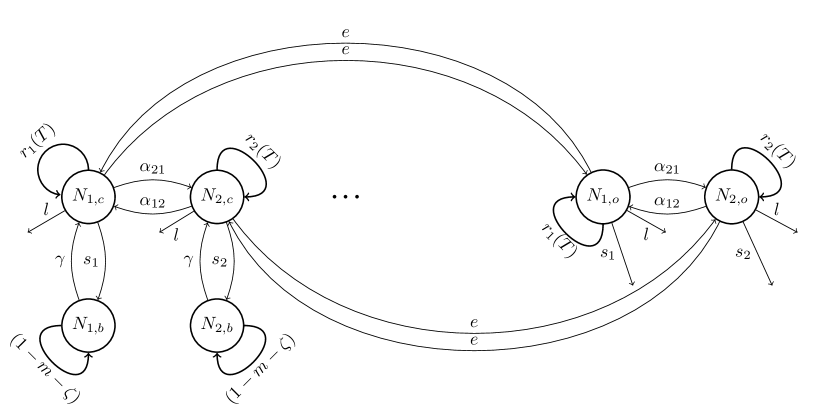
Figure 1: Structure of the model. Phytoplanktonic species (represented by circles) are present in the coast (subscript c), the ocean (o) and the seed bank (b). Parameters governing demography, interactions between organisms and exchanges between compartments are defined in Table 1. Only two species are shown here for the sake of simplicity but 11 species are present in the model.

In this paper, individuals are phytoplanktonic cells that move between the upper layer of coastal water, its bottom layer where a seed bank accumulates in the sediment, and the oceanic zone surrounding the coastal water masses (hereafter “the ocean"). Only oceanic and coastal pelagic cells are subject to BH-density dependence. Resting cells in the seed bank are only affected by mortality $m$ and burial due to sedimentation $\zeta$. Parameters and state variables are defined in Table 1.

Parameter	Name	Value (unit)	Status
$N_{t,i,c/o/b}$	Abundance of species $i$ at time $t$ in the coast ($c$), ocean ($o$), or coastal bank ($b$)	NA (Number of cells)	Dynamic
$T$	Temperature	NA ($K$)	Dynamic
$r_{i}(T)$	Intrinsic growth rate of species $i$	NA (day-1)	Dynamic
$b_{i}$	Thermal decay of species $i$	Field-based ($K^{3}$)	Calibrated
$T_{i}^{opt}$	Optimal temperature for species $i$	Field-based ($K$)	Calibrated
$d$	Daylength	$50$ (%)	Fixed
$\alpha_{ij}$	Interaction strength of species $j$ on $i$ in model I	Field-based (Cells${}^{-1})$	Calibrated
$a_{C}/a_{F}$	Maximum competitive/facilitative interaction strength in model II	Field-based (NA)	Calibrated
$H_{ij}$	Half-saturation for the interaction strength of species $j$ on $i$ in model II	Field-based (Cells$)$	Calibrated
$s_{i}$	Sinking rate of species $i$’s resting cell	$\{0.1;\mathbf{0.3};0.5\}\times\text{Beta}(0.55,1.25)$ (day-1)	Fixed
$e$	Exchange rate between ocean and coast	$\left\{0;\boldsymbol{0.4};0.9\right\}$ (day-1)	Fixed
$l$	Loss rate of pelagic phytoplanktonic cells	$\left\{0.04;0.1;\mathbf{0.2}\right\}$ (day-1)	Fixed
$m$	Resting cell mortality rate	$\mathbf{10^{-5}}$ (day-1)	Fixed
$\zeta$	Resting cell burial rate	$\left\{10^{-3},\mathbf{10^{-2}},10^{-1}\right\}$ (day-1)	Fixed
$\gamma$	Germination $(\gamma_{1})$ $\times$ Resuspension $(\gamma_{2})$ rate	$\left\{10^{-3},\mathbf{10^{-2}},10^{-1}\right\}\times\left\{10^{-5},10^{-3},\mathbf{10^{-1}}\right\}$ (day-1)	Fixed

Table 1: Definition of main state variables and model parameters. State variables and fluctuating parameters are indicated in the last column as “Dynamic”. Parameters that are constant through time are either “Fixed” (directly obtained from literature) or “Calibrated” (obtained through model fitting, with initial values arising from previous studies at the study site). When a range of values is given, the bold numbers indicate the reference values while the others are used for sensitivity analysis. Beta(0.55,1.25) is the Beta distribution with parameters 0.55 and 1.25. For $\gamma,$ germination values for sensitivity analysis were multiplied by the reference value for resuspension, and conversely.

The Beverton-Holt (BH) formulation of multispecies population dynamics, sometimes called Leslie-Gower (Cushing et al., 2004), is a Lotka-Volterra competition equivalent for discrete-time models, and is often used to represent terrestrial plant community dynamics. In our implementation of the model, the population growth rate is modified by both competitive and facilitative interactions, which translates into positive and negative $\alpha_{ij}$ coefficients, respectively. We present two different interaction models. We first use the classical multispecies BH model (model I, eq. 1), also present in the original models of Shoemaker & Melbourne (2016) and Wisnoski et al. (2019). However, the high number of facilitative interactions characterizing the modeled phytoplankton community (Picoche & Barraquand, 2020) combined to the mass-action assumption could have very irrealistic destabilizing consequences, which have been likened to an “orgy of mutual benefaction” (May, 1981): populations grow to infinity because there is no saturation of beneficial effects when density increases. In model I, we therefore forbid the realized growth rate to go above the intrinsic growth rate (its theoretical limit), by setting a minimum value of 1 to the denominator of the BH formulation. We subsequently define saturating interactions, inspired by Qian & Akçay (2020), in our model II (eq. 3). Model II provides a more process-orientated solution to the issue of excessive mutual benefaction (but at the cost of added parameters). Setting a miminum value of 1 to the denominator is still required for large increases or decreases in interaction strengths.

In our framework, the first step of model I can be written as

$$\left\{\begin{array}[]{ccc}N_{t^{\prime},i,c}&=&\frac{\exp(r_{i}(T))N_{t,i,c}}{1+\sum_{j}\alpha_{ij}N_{t,j,c}}-lN_{t,i,c}\\ N_{t^{\prime},i,o}&=&\frac{\exp(r_{i}(T))N_{t,i,o}}{1+\sum_{j}\alpha_{ij}N_{t,j,o}}-lN_{t,i,o}\\ N_{t^{\prime},i,b}&=&N_{t,i,b}(1-m-\zeta)\end{array}\right.$$ (1)

where the intrinsic growth rate $r_{i}(T)$ is a species-specific function of the temperature (see eq. 5), the interaction coefficients $\alpha_{ij}$ are per capita effects of species $j$ on species $i$, and the loss term $l$ accounts for lethal processes such as natural mortality, predation or parasitism. First estimates of interaction coefficients are inferred from a previous study of coastal community dynamics with Multivariate AutoRegressive (MAR) models (Picoche & Barraquand, 2020). We later calibrate these coefficients for model I, since MAR models were applied at a different timescale.

The intrinsic growth rate $r_{i}(T)$ is defined through a modified version of the formula used by Scranton & Vasseur (2016) (eq. 5), which classically decomposes $r_{i}(T)$ in two parts: the species-independent metabolism part $E(T)$ and the species-specific niche part $f_{i}(T)$:

$$r_{i}(T) = E(T)f_{i}(T)$$ (2)

$$\text{where }E(T) = d\times 0.81e^{0.0631(T-273.15)}$$

$$\textnormal{and }f_{i}(T) = \begin{cases}\exp(-|T-T_{i}^{opt}|^{3}/b_{i}),&T\leq T_{i}^{opt}\\ \exp(-5|T-T_{i}^{opt}|^{3}/b_{i}),&T>T_{i}^{opt}.\end{cases}$$

The metabolism part describes the maximum achievable intrinsic growth rate based on Bissinger et al. (2008). This maximum daily intrinsic growth rate is weighted by the daylength $d$ as no growth occurs at night. The realized niche part $f_{i}(T)$ describes the decrease in growth rate due to the difference between the temperature in the environment and the species-specific thermal optimum $T_{i}^{opt}$, and is controlled by the species-specific thermal decay $b_{i}$, which depends on the niche width. It is important to note that unlike $E(T)$, which models direct effects of temperature on metabolism, $f_{i}(T)$ is a phenomenological construct including all indirect effects of temperature, mediated by environmental variables correlated to temperature (light, nutrient inputs, predation, among other environmental conditions). In other words, $f_{i}(T)$ corresponds to a realized niche, pertaining to a given environment, which can be much more narrow than the fundamental thermal niche. Parameterisation is further detailed in Section S1 of the SI.

In model II, oceanic and coastal dynamics are governed by eq. 3:

$$N_{t^{\prime},i,c/o}=\frac{\exp(r_{i}(T))N_{t,i,c/o}}{1+\sum_{j\in\mathbb{C}}\frac{a_{C}N_{t,j,c/o}}{H_{ij}+N_{t,j,c/o}}+\sum_{j\in\mathbb{F}}\frac{a_{F}N_{t,j,c/o}}{H_{ij}+N_{t,j,c/o}}}-lN_{t,i,c/o}$$ (3)

where $a_{C}$ and $a_{F}$ are the maximum competition and facilitation strengths, respectively, with $\mathbb{C}$ and $\mathbb{F}$ the sets of competitors and facilitators of species $i$. We use here similar notations to Qian & Akçay (2020), but use different parameters that vary between species. Indeed, the half-saturation coefficients $H_{ij}$ vary between species, as opposed to the maximum rates in Qian & Akçay (2020). It did not make sense biologically for $H_{ij}$ to be fixed (e.g., in a resource competition context, different species are expected to feel resource limitations at different concentrations of nutrients and at different numbers of competitors). How to shift from MAR- to BH-interaction matrices in model I, and to use the parameter estimates of model I to specify parameters in model II is described in Section S2 of the SI.

After growth and mortality processes occur, exchanges take place between the three compartments, which constitutes the second step of the model (eq. 4):

$$\left\{\begin{array}[]{ccc}N_{t+1,i,c}&=&(1-s_{i}-e)N_{t^{\prime},i,c}+\gamma N_{t^{\prime},i,b}+eN_{t^{\prime},i,o}\\ N_{t+1,i,o}&=&(1-s_{i}-e)N_{t^{\prime},i,o}+eN_{t^{\prime},i,c}\\ N_{t+1,i,b}&=&(1-\gamma)N_{t^{\prime},i,b}+s_{i}N_{t^{\prime},i,c}\end{array}\right.$$ (4)

Each compartment (ocean, coast, coastal seed bank) contains $10^{3}$ cells at the beginning of the simulation, and the dynamics are run for 30 years with a daily time step. We model the temperature input as a noisy sinusoidal signal with the same mean and variance as the empirical data set described below: the amplitude of the sinusoid is 12.4°C and the standard deviation of the noise is 0.25°C.

Parameterization of the models

Literature-derived parameter values

Loss rate

The loss rate $l$ of vegetative cells can be attributed to natural mortality, predation or parasitism. This rate is quite variable in the literature: the model of Scranton & Vasseur (2016) considered a rate around 0.04 day^-1 while a review by Sarthou et al. (2005) indicates a grazing rate of the standing stock between 0.2 and 1.8 day^-1 and an autolysis rate between 0.005 and 0.24 day^-1 (in the absence of nutrients, or because of viral charge). A maximum value of 0.2 is fixed for the model, as a balance between using a high loss rate (probable because of predation) and keeping all species in the community in the reference model (see Section S3 of the SI for more details).

Sinking rate

Phytoplanktonic particles have a higher density than water and cannot swim to prevent sinking (although they are able to regulate their buoyancy, Reynolds 2006). Sinking is mostly affected by hydrodynamics, but at the species-level, size, shape, density-regulation and colony-formation capabilities are key determinants of the particle floatation. In this model, the sinking rate of each species resting cells is drawn from a Beta distribution with a mean value of 9%, and a maximum ($S_{\text{max}}$) around 30%, that is $s\backsim 0.3\beta(0.55,1.25)$ (see Fig. S4), adapted from observations by Passow (1991) and Wiedmann et al. (2016).

Exchange rate

The exchange rate $e$ between the ocean and the coast depends on the shape and location of the coast (estuary, cape, …). Our calibration site is located at an inlet. The flow at the inlet leads to a renewal time of the coastal area water evaluated between 1 and 2.5 days (Ascione Kenov et al., 2015), which corresponds to a daily exchange rate between 40 and 100 %.

Mortality and burial in the seed bank

Loss from the seed bank is the result of cells’ mortality $m$ and their burial by sedimentation $\zeta$. Mortality values range between $10^{-5}$ and $10^{-4}$ per day (more details on the approximation of mortality rates from McQuoid et al. 2002 are given in Section S3 of the SI). However, burial by sedimentation is the prevailing phenomenon. Indeed, once resting cells have been buried, they are not accessible for resuspension even if they could still germinate. Burial depends on the hydrodynamics of the site, but also on biotic processes (i.e., bioturbation) and anthropogenic disturbances such as fishing or leisure activities (e.g., jet skiing). This parameter is thus heavily dependent on the environmental context and varies here between 0.001 and 0.1 per day.

Germination/resuspension

Both germination ($\gamma_{1})$ and resuspension ($\gamma_{2}$) are needed for resting cells to contribute to the vegetative pool in the water column ($\gamma=\text{resuspension$\times$germination})$. As actual rates of germination are not easily deduced from the literature, a set of credible values has been tested (1%, 0.1%, 0.01%). Similarly, resuspension values are seldom computed for phytoplanktonic cells, but models for inorganic particles can be used (see Section S3 of the SI for literature and details). In this paper, we explore values between $10^{-5}$ (stratified water column) to 0.1 (highly mixed environment).

Initial interaction matrix

Initial values of interaction strengths between species are based on Multivariate AutoRegressive (MAR) model estimates (Picoche & Barraquand, 2020). MAR(1) models relate the log-abundance of each of the $S$ phytoplankton species at time $t+1$ to log-abundances of all species at time $t$, through an interaction matrix, and effects of abiotic variables at time $t+1$ (see Section S2 of the SI). Interactions are estimated only between species within the same trophic level, and are independent from the environmental variables that were included in the MAR model estimates as covariates, such as temperature in our case. This allows to remove at least some of the confounding factors, such as seasonality. A phylogeny-based interaction matrix resulted in a better fit to model the community dynamics, i.e. pennate/centric diatoms only interact with other pennate/centric diatoms, respectively, and dinoflagellates only interact with dinoflagellates.

The MAR model can only estimate apparent interaction strengths: complex processes can be at work behind values of competition and facilitation, either from abiotic (e.g., hydrodynamics) or biotic (e.g. consumption by predators or parasites) variables. For more consideration on apparent interactions detected in phytoplankton communities with the MAR model, we refer the reader to Barraquand et al. (2018). In the present model, while we tune interaction strength values (see below), the type of interaction (competition, facilitation or absence of interaction) remains the same as computed in Picoche & Barraquand (2020).

Parameter calibration

As explained above, we use initial interaction estimates from our previous time series modelling (Picoche & Barraquand, 2020, see Section S3 of the SI for the equations), which are then calibrated to the time series (thus possibly re-estimated, see below), to take into account the differences in model structure and timescale between this study and Picoche & Barraquand (2020). In SI Section S3, we present the formulas relating the MAR interaction coefficients to the Jacobian matrices of the Beverton-Holt multispecies models, as these formulas allow to obtain proper $\alpha_{ij}$ coefficient values.

The calibration procedure consists in launching 1000 simulations, each characterized by a specific set of interaction coefficients. More precisely, for each simulation, an interaction coefficient ($\alpha_{ij}$ in model I, $H_{ij}$ in model II) has probability $1/5$ to keep its present value, probability $1/5$ to increase by 10% , $1/5$ to decrease by 10%, $1/5$ to be halved and $1/5$ to be doubled. The numbers of coastal pelagic cells (which are the ones measured empirically) are then extracted over the last 2 years of the simulation, and compared to observations using the following summary statistics:

• average abundance $f_{1}=\sqrt{\frac{1}{S}\sum_{i}^{S}\left(\bar{n}_{i,obs}-\bar{n}_{i,sim}\right){}^{2}}$ where $S$ is the number of taxa and $\bar{n_{i}}$ is the logarithm of the mean abundance of taxon $i$.

• amplitude of the cycles $f_{2}=\sqrt{\frac{1}{S}\sum_{i}^{S}\left[\left(\max(n_{i,obs})-\min(n_{i,obs})\right)-\left(\max(n_{i,sim})-\min(n_{i,sim})\right)\right]{}^{2}}$ where $n_{i}$ is the logarithm of the abundance of taxon $i$.

• period of the bloom. The year is divided in 3 periods, i.e. summer, winter and the spring/autumn group (as taxa blooming in these periods can appear in either or both seasons). We give a score of 0 if the simulated taxon blooms in the same period as its observed counterpart and 1 otherwise.

Simulations with taxon extinction (i.e., the taxon is absent for more than 6 months in a compartment) are discarded, as extinctions are not observed in the field data. Parameter sets are then ranked according to their performance for each summary statistic, and we select the set of interactions minimizing the sum of the ranks.

Sensitivity analysis

Parameters taken from the literature may be site- or model- specific, or vary over several orders of magnitude in the literature, e.g., rates of sinking $s$, resuspension/germination $\gamma$, seed burial $\zeta$, and loss of pelagic cells $l$. We therefore performed a sensitivity analysis to these highly uncertain parameters. The set of tested values for each parameter is given in Table 1. We used average abundances and amplitudes at the community and taxon levels for the last 2 years of simulations as the major model diagnostics.

Empirical dataset used for calibration

The models are calibrated using time series of phytoplanktonic abundances that have been monitored biweekly for 21 years in the Marennes-Oléron Bay, on the French Atlantic Coast (the Auger site analysed in Picoche & Barraquand, 2020). We stress that we are not trying to model precisely this particular community, but rather to constrain our models with an empirically-derived interaction network and species-specific thermal niches, which helps to produce lifelike patterns of phytoplankton community dynamics resembling observable data (seasonal dynamics, high-amplitude blooms, differences in average abundances matching data).

Scenarii

The effect of the seed bank on biodiversity and community dynamics can be evaluated through the response to disturbance with and without the resting-stage compartment. Mortality in the seed bank is set to 100% to effectively remove the compartment. We evaluate two main disturbances:

1. increase or decrease in interaction strength

2. temperature change, either in mean value or variability

In the first scenario, interaction strengths are multiplied or divided by a factor ranging between 1 and 10. In order to differentiate the effects of facilitative and competitive interactions on coexistence, we vary only one type of interactions at a time. Here, both intra and interspecies interactions are modified; we present in Section S6 of the SI additional simulations with a change in interspecies interactions only.

In the second scenario, five different climate change trajectories are assessed. In the first three, the average temperature is increased by 2, 5, or 7°C (Boucher et al., 2020). In the next two, keeping the reference average temperature, the total variance of the temperature, including seasonality and noise, is either decreased or increased by 25%. Each climate change trajectory is run 5 times to account for the intrinsic stochasticity of the temperature signal.

In both scenarii, simulations are run for 30 years for both population growth models, with and without a seed compartment, and only the last 2 years are considered to evaluate effects of changes in parameters and in temperature. The code for all simulations is to be found at https://github.com/CoraliePicoche/SeedBank.

Results

Phytoplankton dynamics

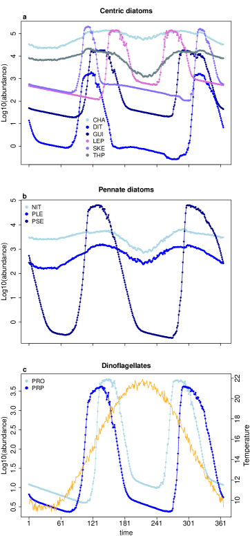
Figure 2: Simulated phytoplankton dynamics for a year in model I (time in days). Each panel corresponds to a cluster of interacting taxa: centric diatoms (a), pennate diatoms (b) and dinoflagellates (c). Taxa only interact within their cluster of related taxa (see Methods). The orange line in the third panel indicates the temperature.

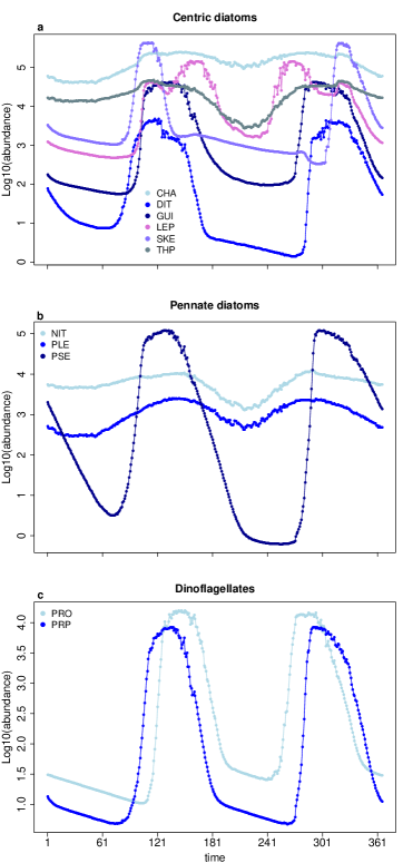
Figure S5: Simulated phytoplankton time series for a year in model II (with saturating interactions). Each panel corresponds to a cluster of interacting taxa: centric diatoms (a), pennate diatoms (b) and dinoflagellates (c). Taxa only interact within their cluster (see Methods in main text).

The classical mass-action (model I) and saturating interaction (model II) formulations of multispecies dynamics both reproduced the main characteristics of observed phytoplankton dynamics. They produced one or two blooms during the year and a range of abundances covering several orders of magnitude, with the right timing of the blooms. At the Auger site that was used for calibration, abundances increase in spring and can last over part of summer, or start a new bloom in autumn, which is what we observed as well in the models. Annual mean abundance of the various species was also well reproduced. That said, in some cases, abundances could be lower than expected and the variation in abundances due to seasonality was underestimated (Fig. 2). In all cases, saturating interactions led to higher abundances than mass-action interactions throughout the year (Fig. S5).

Sensitivity to uncalibrated parameters

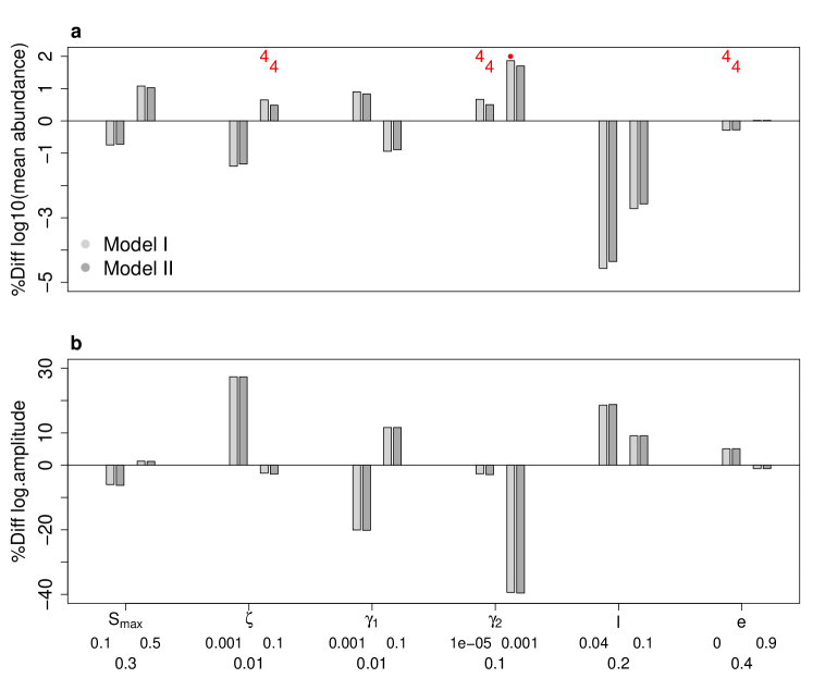
Figure 3: Sensitivity of the model to variation in parameters, measured as the difference between the reference simulation metric and the metric for the simulation including a change in parameter. The two metrics used were the decimal log average abundance (a) and the decimal logarithm of the ratio between maximum and minimum abundance (b) of the coastal phytoplanktonic community. The x-axis is divided in three rows: the symbol of the parameter defined in Table 1 (first row), values used in the sensitivity analysis (second row) and values used in the reference simulation (third row). Numbers in red in the top panel are the final number of species in the ocean and dots correspond to simulations in which at least one species abundance reached 0 at one point but the species did not disappear.

Phytoplankton abundances were not strongly affected by changes in the parameter values (Fig. 3). As parameters were varied in their plausible range, the average change in mean abundance on the coast between the reference simulation and the sensitivity simulations varied between -4.6 and 1.9% for model I and between -4.4 and 1.7% for model II, with similar deviations (same sign and magnitude) in the two models.

In the two models, the decrease in mortality rate of vegetative cells $l$ had the highest impact on the final average abundance, leading to an increase in abundances. The exchange rate between the ocean and the coast had a much lower effect on the coastal average abundance.

On the other hand, the amplitude (i.e., decimal logarithm of the maximum to minimum ratio of abundance) was more affected by changes in parameters and could vary by -39.6 to 18.8% in model I, and between -39.6% and 18.8% in model II. Results were qualitatively the same in the two models, with a decrease in resting-stage burial being the main driver of the decrease in amplitude, and a decrease in resuspension leading to an increase in amplitude.

In three cases (burial rate set to 0.1, resuspension set to 10^-5 or exchange rate set to 0), the final richness of the oceanic community decreased from 11 to 4. Extant species were the same in all simulations (CHA, THP, NIT, PLE, i.e. temperature generalist species; the correspondence between codes and groups of species is given in Section S4 of the SI). When resuspension was set to 0.001, a species periodically disappeared from the ocean, to be subsequently re-seeded by the coastal population.

For all parameters, except the sinking rate, an increase in mean abundance was associated to a decrease in amplitude.

Scenarii of environmental change

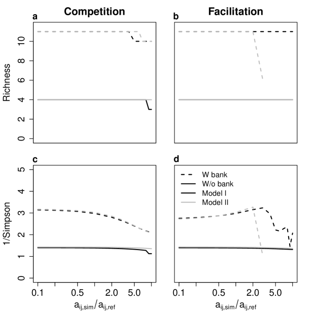
Figure S6: Measures of biodiversity in the ocean at the end of the simulation: a-b) richness and c-d) inverse of the Simpson index, with (dashed line) and without (solid line) a seed bank, as a function of the strength of competition and facilitation with a classical Beverton-Holt (black lines) or a saturating interaction (grey lines) formulation, keeping the same values for the intraspecific interaction strengths. The x-axis shows the factor by which each interaction coefficient was multiplied, e.g. the value 0.1 indicates that the interaction strengths in the simulation are 10 times lower than the interactions strengths in the reference simulation. Note the logarithmic scale.

Two scenarii were designed to test the buffering effect of the seed bank against disruption. In both cases, it consisted in removing the seed bank by setting resting-stage mortality to 100% per day. Without any other disturbance to the system, this led to a decrease in richness from 11 to 4 species at the end of the simulation (Fig. S6) while the total abundance of phytoplankton was not strongly affected (around $10^{5}$ in all cases). The inverse of the Simpson index (the second Hill number) decreased from approximately 3 to 1, showing that the disappearance of the seed bank did not affect only the rarest species.

Biotic effects

Figure 4: Measures of biodiversity in the ocean at the end of the simulation: a-b) richness and c-d) inverse of the Simpson index, with (dashed line) and without (solid line) a seed bank, as a function of the strength of competition and facilitation with a classical Beverton-Holt (black lines) or a saturating interaction (grey lines) formulation. The x-axis shows the factor by which each interaction coefficient was multiplied, e.g. the value 0.1 indicates that the interaction strengths in the simulation are 10 times lower than the interaction strengths in the reference simulation. Note the logarithmic scale.

Our first hypothesis was that the absence of the seed bank would cause the community to be more affected by a higher competition strength. Counter-intuitively, our results (Fig. S6) showed that an increase in competition strength only had negative effects with model I, and for high competition values (6 times the reference ones at least), shifting from 4 to 3 species in the oceanic compartment of a community without a seed bank. By contrast, an increase in competition strength did not affect the richness of a community with a seed bank. On the contrary, a decrease in competition (from a factor 0.5 and lower) or an increase in facilitation (starting from a factor 2 and higher) led to much smaller communities in model II in the presence of a seed bank.

The inverse of the Simpson index was also affected by the changes in interaction strengths, with similar patterns to richness, as it was lowest for high facilitation or low competition. Some species reached very high growth rates in these scenarios, which then fed back onto community dynamics, generating lower diversity in the end.

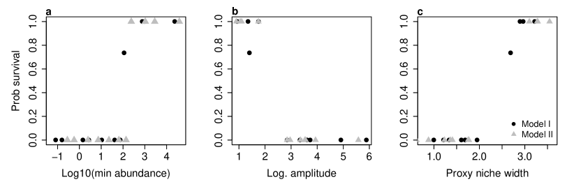
Figure 5: Probability of survival of species along a gradient of competition strength and in the absence of a seed bank, as a function of their population dynamics characteristics (minimum abundance, logarithm of amplitude and niche width) in the reference parameter set. Each dot corresponds to a species, and its survival using model I (black) or model II (grey).

Species which disappeared were characterized by a lower minimum abundance, a higher amplitude of fluctuations and a small niche (Fig. S7). However, their interactions were not qualitatively different from the other species.

Abiotic effects

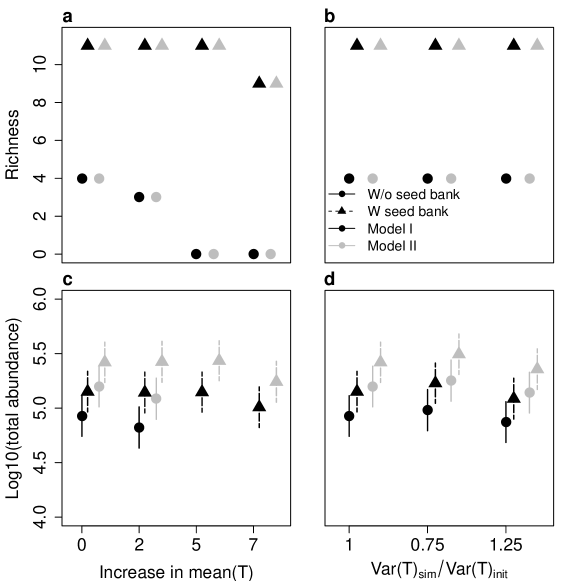
Figure 6: Variation in richness and total abundance with and without a seed bank as a function of the mean (left) and variance (right) of the temperature with a mass-action (black line, model I) or a saturating interaction (grey line, model II) formulation.

Our second hypothesis was that the absence of a seed bank would reduce the ability of a community to withstand changes in its abiotic environment, here represented by variation in the temperature. This was true for both models (Fig. 6), as the communities without a seed bank could not maintain their richness with an increase in temperature above 2°C, as opposed to communities with a seed bank, which could only be affected by a 7°C increase (scenario SSP5 8.5, Boucher et al. 2020). In all cases however, the total abundances were not strongly affected. Indeed, the total abundance of a community is driven by a small number of numerically dominant species, which did not disappear. High total abundances tended to correspond to the abundance of only one or two species. Model II consistenly led to higher abundances, as was already the case in the reference simulations.

The variance of the temperature did not affect richness nor total abundance of communities with a seed bank. This was also true without a seed bank. The presence of resting stages did increase total abundance though.

Some additional simulations were made to better understand the functioning of the model, during which the temperature was kept constant (equal to the average temperature of the fluctuating environment). For a constant and average temperature, the presence of a seed bank did not change the final richness of the communities. There were 9 extant species at the end of the constant-environment simulations, whether there was a seed bank or not. The two specialist species whose thermal optima were farthest from the constant temperature went extinct even when the seed bank was present, since the environmental fluctuations allowing them to benefit from cold or warm temperature were removed. The other species benefited from the constant environment, as 9 species instead of 4 persisted in the case where the seed bank was removed (see below for a discussion). The high persistence in a constant environment (9 out of 11) translates the stabilizing, data-driven interaction structure of our model. For both models I and II, the dynamical system reached a fixed point equilibrium in absence of the fluctuations induced by a variable temperature.

Discussion

Using a meta-community model which accounts for exchanges between the ocean and the coast, as well as movements between the top and the bottom of the coastal water column, we were able to show that a resting stage, leading to the formation of a seed bank, can help maintain biodiversity. Our phytoplanktonic community dynamics model was parameterized based on literature, field-based phenology, and interaction strength estimates. It was then calibrated on phytoplankton community time series. Our model was able to simulate realistic community dynamics (both mean abundances and temporal patterns), while including the effects of both positive and negative interactions on community dynamics. When removing the seed bank, biodiversity decreased drastically. The total abundance of the community decreased as well. This was true for the reference parameter values, as well as when species interaction strengths and environmental fluctuation levels were altered, in which cases the seed bank’s buffering influence disappeared. Moreover, when faced with a biotic or abiotic perturbation, communities where species could divert part of their population to a dormant stage were less prone to species loss and could maintain their biomass through the years. These results were consistent for the two interaction models that we considered, with and without progressive saturation in interaction strengths. Our results therefore demonstrate the major potential role of phytoplanktonic resting stages in maintaining biodiversity. These results align with the findings of previous theoretical studies, that have put forward similar effects of dormant stages in other taxa, such as plants (Levine & Rees, 2004; Jabot & Pottier, 2017), invertebrates (Wisnoski et al., 2019) or (smaller) microbes (Jones & Lennon, 2010).

The positive effect of a seed bank on species diversity in our model is contingent upon environmental fluctuations. Indeed, in a constant environment, the absence of a seed bank did not alter persistence, and final richness was higher than in a fluctuating environment (9 species in a constant environment vs. 4 species in a variable environment, both without a seed bank). The absence of abiotic perturbations of the intrinsic growth rates enabled species which were not too far from their thermal optima to maintain. This might be surprising for readers acquainted with Hutchinson’s nonequilibrium theory (Hutchinson, 1961). However, the theoretical literature on persistence in variable environments has shown that additional mechanisms (reviewed in Fox, 2013) are needed to maintain diversity in the long run, such as relative nonlinearities or the storage effect, which is at least absent from the pelagic part of our model due to the absence of buffered growth (see Section S8 in SI). There is a clear destabilizing effect of environmental variation in our model without the seed bank, which is probably heightened by the fact that environmental variation is positively autocorrelated through seasonality (Picoche & Barraquand, 2019; Schreiber, 2021). Although the storage effect could manifest itself when combining pelagic and seed bank parts of our model, it is very unlikely to be at play here as environmental conditions do not impact recruitment rates in our model, while this is usually a requirement for the storage effect to manifest in such models (Chesson, 2003).

Even in the absence of a storage effect, however, the high longevity of the resting stage itself can explain the effect of the seed bank in a fluctuating environment. Such longevity is due to dormancy, which has long been observed in field and experimental data, including for phytoplanktonic organisms (Eilertsen & Wyatt, 2000), and has been theorized to be an important and neglected process in the wider microbiology literature (Locey, 2010; Jones & Lennon, 2010). It allows recolonization of a community where counts of pelagic cells alone would suggest that some species have gone extinct. This colonization-in-time may of course combine with present recolonization from other spatial areas, as is known for plants (Shmida & Ellner, 1984). In our case, our focus on phytoplankton led us to assume that organisms moved between the coast and the ocean, which were largely synchronous environments. Spatial recolonization was therefore less important than temporal recolonization; the relative importance of the two processes may vary depending on the organisms and the degree of spatial synchrony of their environment (in plankton, see Montresor et al. 1998; Anderson et al. 2005).

The specificities of phytoplankton resting stages, that usually fall to the ocean bottom in coastal areas, led us to assume that only the “vegetative” stage (here, the classic pelagic form of planktonic cells) disperse. In some other metacommunity models with dormant seed banks (e.g. Wisnoski et al., 2019), the dormant stage can disperse as well. This would be true for most plants too (and perhaps some phytoplankters in situations where they are transported by animals). However, the restriction about which stage can move did not change the general conclusion already stated by Wisnoski et al. (2019): the combination of spatial dispersal and dormancy through seed banks greatly helps biodiversity maintenance. In our study, this main result was also robust to changes in exchange parameters and mean interaction values in the community.

Species persistence varied between the coastal and oceanic compartment. Temporary species disappearance could happen periodically in the ocean but species were able to reinvade from the coast, thanks to the connection of the coast to the seed bank. Local extinction in the absence of a seed bank confirms conclusions from Hellweger et al. (2008) on a single species. This suggests that some species may be locally transient: they are filtered out from certain patches, but can reinvade more or less periodically the environment (as found by Guittar et al. 2020, for grasslands).

Survival probabilities of species within the community in the absence of a seed bank also depended on their characteristics – and therefore species rescued by the seed bank also have specific characteristics. While extinct species growth rates tended to be less affected by interactions for average densities (Fig. S7 in SI), such species had higher amplitudes of population variation as well as a smaller niche width. Specialists species, growing at specific temperatures, therefore typically benefit the most from a seed bank.

Despite the evidence for seed bank effects that we and others uncovered, phytoplanktonic community models designed to explain biodiversity usually avoid modelling seed banks. In our view, this may decrease the possibility of spontaneous re-colonization at the coast (at very low densities initially), which can then spill to the open ocean by progressive dispersal by the currents. Ignoring the seed bank may also decrease overall persistence, as fitting models I and II without a seed bank does not allow all species to persist here. If the goal of a community-level model is very short-term prediction (days, weeks), this recolonization can probably be neglected, and there are no risks of extinction over these short time frames. However, over multiple years, ignoring cryptic life stages allowing recolonization could strongly bias downwards our view of long-term coexistence. Long-term phytoplankton coexistence modelling (over multiple decades or more) likely requires that we take into account resting stages, whose influence may become only more important as the timescale increases, due to the very long possible dormancies that have been evidenced (Ellegaard & Ribeiro, 2018; Sanyal et al., 2022). When modelling different stages of the life cycle in a detailed manner – as done here – is impractical, the recolonization could perhaps be simplified to a stochastic immigration term (as done in Stock et al. 2005 in a single-species context). This technical suggestion certainly extends to models of (terrestrial) plant community dynamics.

More research on dormant stages may be needed to parameterize truly predictive mechanistic phytoplankton models with multiple life stages, in particular to inform parameters such as the sinking rate of resting cells, as well as burial and resuspension parameters. These parameters are all linked to hydrodynamics (Yamamoto et al., 2002; Yñiguez et al., 2012) and may locally vary. Sinking rates show an interesting conflict between short- and long-term survival: in coastal areas, a fraction of sinking cells contribute to the seed bank, increasing the odds of species long-term survival at the cost of short-term individual cell survival. But high sinking rates are essentially “wasted” in the open ocean – whether different sinking rates can be selected, to some degree, by such different environments could be quite revealing. How cells get up rather than down in water column might be as interesting but more difficult to study. The likely idiosyncratic nature of recolonization by resting cells – due to the contingency on local hydrodynamics – means that experimentation might be the only manner in which the frequency of reinvasion can be assessed. Currently, one of the only recolonization-related parameters measured in the field is the rate of survival of the cells found in the sediment (Montresor et al., 2013; Solow et al., 2014). While very important, this parameter is a necessary not sufficient condition for reinvasion of the population at future times. We need more information about the abilities of resting cells buried in the sediment to come up to the pelagic zone, which is required for recolonization to actually occur. Many factors may contribute: bottom currents, benthic animals,… We therefore encourage both experiments and field observations to follow actual seed trajectories, in order to help us understand this cryptic part of the diversity maintenance process.

Declaration of Competing Interest

The authors declare that they have no known competing financial interests or personal relationships that could have appeared to influence the work reported in this paper.

Author contribution statement

CP and FB designed the project and the models. CP wrote the computer code and produced the figures. CP and FB interpreted the results and wrote the manuscript.

Acknowledgements

We thank Nathan Wisnoski and Frank Jabot for useful feedback. FB and CP were supported by grants ANR-10-LABX-45 and ANR-20-CE45-0004. CP was supported by a PhD grant from the French Ministry of Research.

Supporting Information for Seed banks can help to maintain the diversity of interacting phytoplankton species by C. Picoche & F. Barraquand. (doi:10.1016/j.jtbi.2022.111020)

S1 Intrinsic growth rate modeling

The intrinsic growth rate can be decomposed in 2 elements:

$$r_{i}(T)=E(T)f_{i}(T)$$ (5)

with $E(T)$ the response to temperature common to all species and $f_{i}(T)$ the species-specific response. This section provides detailed information regarding $E(T)$ and $f_{i}(T)$ estimates.

Common response to temperature

Phytoplanktonic growth rates cover a broad range of values: between 0.2 and 1.78 day^-1 for diatoms in Reynolds (2006), even reaching 3 day^-1 in the meta-analysis of 308 experiments by Edwards et al. (2015). These values are often computed from measurements on isolated species or on small communities in laboratory conditions, in a constant environment. A broader perspective is therefore necessary to understand general responses to changes in the environment (Bissinger et al., 2008; Edwards et al., 2016), especially temperature.

We first used the equation by Scranton & Vasseur (2016) as a starting point, but it was not able to reproduce the observed values found in Edwards et al. (2015) (see low values of the growth rate in Fig. S1a, between 0.05 and 0.8, in place of values between 0.2 and 3 day^-1). In this context, we decided to use the formula by Bissinger et al. (2008) to compute the maximum growth rate response to the temperature. There are two reasons for this choice. First, their model is a general function that can be applied to all species. Second, Bissinger et al. (2008) is an update of the seminal work of Eppley (1972) (which was used in Scranton & Vasseur, 2016, but might be outdated).

The relationship between temperature and growth rate is then $E(T)\thinspace=\thinspace 0.81\exp^{0.0631(T-273.15)}$, with $T$ in Kelvin degrees. In this case, growth rates vary between 0.81 and 3.9 day^-1 for temperatures between 0 and 25°C, in line with previous observations. However, these daily growth rates need to be proportional to the daylength as no growth occurs at night: we therefore divide $E(T)$ by two in our models.

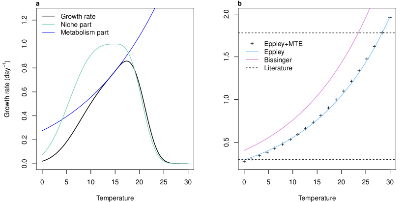
Figure S1: Decomposition of the Scranton & Vasseur (2016) growth rate formula (a). The black line indicates the final growth rate with their model. The blue line corresponds to the species-specific response to temperature for a thermal optimum of 15°C and the green line is the maximum achievable growth rate, a composite of the metabolic theory of ecology (MTE) and the formula by Eppley (1972). This formula is shown by black crosses in (b) and compared to the Eppley (1972) curve in blue and Bissinger et al. (2008) formula in purple. Horizontal lines show limits found in the literature (Reynolds, 2006).

Species-specific response to temperature

The niche part of the growth rate $f_{i}(T)$ is mainly defined by two parameters which drive the phenology of a species: the thermal optimum $T_{i}^{opt}$ and a proxy of the niche width $b_{i}$ (eq. 6).

$$f_{i}(T)=\begin{cases}\exp(-|T-T_{i}^{opt}|^{3}/b_{i}),&T\leq T_{i}^{opt}\\ \exp(-5|T-T_{i}^{opt}|^{3}/b_{i}),&T>T_{i}^{opt}\end{cases}$$ (6)

The annual dynamics of phytoplanktonic organisms is usually characterized by a blooming period and a lower concentration during the rest of the year. The bloom can be triggered by a combination of nutrient and light input, as well as a sufficient temperature. All these variables being more or less correlated to the seasonal rythm, it is reasonable to restrain this study to the effect of one variable, temperature. Thus, the niche computed here is not the fundamental thermal niche, but a composite of all environmental conditions covarying with the temperature and promoting population growth. Such environmental conditions of course include solar irradiance which is strongly correlated to temperature in the field, but could also account for other factors, such as predation, that have a seasonal rythm which is partly captured by temperature. The niche part of the growth rate $f_{i}(T)$ therefore describes the realized niche of species $i$, not its fundamental niche.

We base our estimates of $T_{i}^{opt}$ and $b_{i}$ on field observations. For each taxon and each year, we define the beginning of the bloom as the date when the taxon abundance exceeds its median abundance over the year. The duration of the bloom is the number of days between the beginning and the date where abundance falls below the median value. Taxa are then separated into two groups. In the field, generalists are characterized by one long bloom in the year or several blooms during which the abundances oscillate around their median. Specialists tend to appear only once or twice in the year for shorter amounts of time. A genus is therefore defined as a generalist if the duration of its cumulated bloom days over a year last more is above the average duration of all blooms (137 days) for at least 15 years over the 20 years of the time series, and as a specialist if they fall below this threshold.

In the models, we assume that generalists have a niche width between 15 and 30° and specialists, between 5 and 10°. In order to compute $b_{i},$ we make the additional assumption that temperatures outside of this range lead to a growth rate at least 10 times inferior to the growth rate obtained at their thermal optimum ($\exp(-|7.5|^{3}/b_{i}=0.1$ for a niche width of 15°). This leads to values of $b_{i}$ between 180 and 1500 for generalists, and 7 and 55 for specialists. A set of $b$ values is drawn from a uniform distribution within these boundaries. Meanwhile, taxa are ordered as a function of the mean cumulated bloom length and larger niche values are attributed to longer mean bloom length, i.e. $\sum\overline{L}_{i}>\sum\overline{L}_{j}\Rightarrow b_{i}>b_{j}$ where $\overline{L}$ is the mean over 20 years of the annual cumulated bloom lengths.

The thermal optimum $T_{i}^{opt}$ was first defined as the mean minimum temperature of the bloom throughout the whole time series. However, this value led to blooms occuring mainly in the winter and needed to be increased by 5° in order to simulate realistic phytoplankton cycles.

It should be noted that a variation in niche width also affects the final shape of thermal preferences. Indeed, when $b_{i}$ increases, the niche term $f_{i}$ has smaller variation in values around the thermal optimum. In this case, the final value of the growth rate is driven by the metabolism part of the equation (Fig. S2).

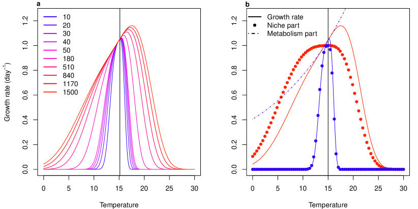
Figure S2: Relationship between daily growth rates and temperature with different values of niche width $b$ (whose values are indicated in the legend, corresponding to specialist and generalist species) and the same thermal optimum, 15°C, indicated by the solid black line (a). On the right panel, only the two extreme values of $b$ (10 and 1500) are shown in blue and red respectively. Solid lines then correspond to the final growth rate, points correspond to $f_{i}(T)$ values (see eq. 5) and the dotted line corresponds to $E(T)$ values.

We show the growth rates $r_{i}(T)$ as a function of temperature for each modeled taxon below (Fig S3).

Figure S3: Growth rate as a function of temperature for the taxa used in the model (names are defined in Table S2).

S2 Initial estimates of interaction values

Model I: Lotka-Volterra interactions

Interactions between taxa have previously been computed with a Multivariate AutoRegressive model (eq. 7, Picoche & Barraquand, 2020).

$$\mathbf{n}_{t+1}=\mathbf{B}\mathbf{n}_{t}+\textbf{C}\textbf{u}_{t+1}+\mathbf{e}_{t},\mathbf{e}_{t}\thicksim\mathcal{{N_{S}}}(0,\mathbf{Q})$$ (7)

where $S$ is the number of taxa, $\mathbf{n}_{t}$ is the $S\times 1$ vector of log-abundance of phytoplankton taxa, $\mathbf{B}$ is the $S\times S$ interaction matrix with elements $b_{ij}$ (the effect of taxon $j$ on taxon $i$), $\mathbf{C}$ is the $S\times V$ environment matrix describing the effects of variables $\mathbf{u}_{t+1}$ on growth rates and the noise $\mathbf{e}_{t}$ is a $S\times 1$ noise vector following a multivariate normal distribution with a variance-covariance matrix $\mathbf{Q}$. The interaction model we use in the present paper is a Beverton-Holt multispecies model (eq. 1 in main text), also called at times Leslie-Gower. In Picoche & Barraquand (2020)’s Supporting Information, we showed that MAR and BH interaction coefficients, respectively $b_{ij}$ and $\alpha_{ij}$, could map once abundances at equilibrium $N_{i}^{*}$ are defined.

$$\begin{cases}b_{ii}-1=&\frac{-\alpha_{ii}N_{i}^{*}}{1+\sum_{l}\alpha_{il}N_{l}^{*}}\\ b_{ij,i\neq j}=&\frac{-\alpha_{ij}N_{j}^{*}}{1+\sum_{l}\alpha_{il}N_{l}^{*}}\end{cases}$$

Let’s define $\tilde{b}_{ij}$ with $\tilde{b}_{ii}=b_{ii}-1$, and $f_{A}(i)=\sum_{l}\alpha_{ij}N_{l}^{*}$.

$$\tilde{b}_{ij}(1+f_{A}(i))=-\alpha_{ij}N_{j}^{*}$$

We then sum on columns (on $j$):

$$\sum_{j}[\tilde{b}_{ij}(1+f_{A}(i))]=-f_{A}(i)$$

$$\Leftrightarrow-f_{A}(i)(1+\sum_{j}\tilde{b}_{ij})=\sum_{j}\tilde{b}_{ij}$$

$$\Leftrightarrow f_{A}(i)=-\frac{\sum_{j}\tilde{b}_{ij}}{(1+\sum_{j}\tilde{b}_{ij})}$$

$$\Leftrightarrow\alpha_{ij}=-\frac{1}{N_{j}^{*}}\tilde{b}_{ij}(1-\frac{\sum_{j}\tilde{b}_{ij}}{1+\sum_{j}\tilde{b}_{ij}})$$

$$\Leftrightarrow\alpha_{ij}=-\frac{1}{N_{j}^{*}}\frac{\tilde{b}_{ij}}{1+\sum_{j}\tilde{b}_{ij}}.$$

This gives an exact correspondence between $\alpha_{ij}$ and $b_{ij}$. In the multispecies BH model, the presence of mutualistic interactions can lead to an orgy of mutual benefaction (May, 1981). We impose a minimum value of 1 to the denominator of the BH formulation, meaning that the growth rate cannot be higher than the maximum growth rate calculated, $r_{i}(T)$.

Model II: saturating interactions

We now move to a model with saturating interactions between taxa:

$$N_{t+1,i}=\frac{e^{r_{i}(T)}N_{t,i}}{1+\sum_{j/a\in\mathbb{C}}\frac{a_{C}N_{t,j}}{H_{ij}+N_{t,j}}+\sum_{j/a\in\mathbb{F}}\frac{a_{F}N_{t,j}}{H_{ij}+N_{t,j}}}$$ (8)

where coefficients $a_{C}$ and $a_{F}$ are the maximum interaction strengths for competition and facilitation, respectively, $H_{ij}$ is the abundance of taxon $j$ to reach half of the maximum effect of taxon $j$ on taxon $i$, and $\mathbb{C}$ and $\mathbb{F}$ are the sets of competitive and facilitative interactions. This formula can be linked to the Unique Interaction Model by Qian & Akçay (2020), i.e., each taxon provides a unique type of benefit or disadvantage to the focus taxon.

There is no single solution for matching the $\mathbf{B}$ matrix of the MAR model to model II including $H_{ij}$, $a_{C}$ and $a_{F}$. We approximate the maximum interaction strength $a_{C}$ as the average sum of all taxon effects $\alpha_{ij}N_{j}$ exerted on a given taxon if all interactions were competitive (eq. 9). To compute $a_{F}$, we make two assumptions: on average, a) there is 70% facilitation in our dataset and b) the realized growth rate on a log-scale should not exceed $r_{i}(T)$, as in model I. We consider that the relationships that apply to individual interactions $\alpha_{ij}$ should also apply to the saturation point (eq. 10), so that:

$$a_{C} = \frac{1}{S}\sum_{i}\left(\sum_{j}|\alpha_{ij}|N_{j,\text{max}}\right)$$ (9)

$$(1-0.7)a_{C}+0.7a_{F} = 0$$ (10)

where $N_{j,\text{max}}$ is the maximum observed abundance of species $j$. We use $N_{j,\text{max}}$ and the absolute value of interactions $|\alpha_{ij}|$ (i.e., all interactions are considered competitive in this case) to make sure that we maximise $a_{C}$.

At low abundances, we can consider that interactions are far from saturation. Taking the tangent of the function at this point, $H_{ij}$ can be approximated by $f\frac{a_{C/F}}{\alpha_{ij}}$, where $f=2$ is a correction factor that takes into account the fact that the slope at origin for the type II response is likely higher than the slope for a linear effect of density.

S3 Choice of parameters derived from literature

This section contains additional information on “fixed” parameter definitions (i.e., parameter not estimated from field data) and their chosen values. Note that these values are then subjected to sensitivity analysis, where by definition they are modified.

Loss rate

The loss rate corresponds to multiple mortality processes. The Lotka-Volterra model of Scranton & Vasseur (2016) considered a rate around 0.04 day^-1. In Jewson et al. (1981), washout (0.5%), parasitism (4% of cells are infested and die) and grazing still remained low (about 0.05%) when compared to growth rates. Li et al. (2000) found values between 0.02 and 0.1 day^-1 for natural mortality only, while a review by Sarthou et al. (2005) indicated a loss of daily primary productivity around 45% due to grazing only, while cell autolysis only can lead to a loss rate between 0.005 and 0.24 day^-1 (in the absence of nutrients, or because of viral charge). Cumulating both natural mortality (cell autolysis) and grazing, we know that maximum rates should be above 0.24 day^-1. Trying to make a compromise emerge from the literature above, given that we are not always at the maximal loss rates, we set the reference value to 0.2 day^-1. This strikes a balance between acknowledging all sources of mortality and the need to keep all species in the reference model.

Sinking rate

Among the hydrodynamics processes that drive the sinking rate, turbulence and eddies – themselves driven by tidal currents, the shape of the coast or wind conditions – are influential in keeping the cells at the top of the water column. For that reason, laboratory experiments on sinking rates are not sufficient to calibrate a field-based model. We therefore chose sinking rate values from field studies. In the Gotland Basin (central Baltic Sea), Passow (1991) measured a large variability in sinking rates, even within the same genus (e.g., between 1 and 30% for Chaetoceros spp.). However, a pattern could be highlighted, with a small number of genera that sank more than the rest of the community. The mean sinking rate for Chaetoceros and Thalassiosira was around 10% while it was around 1% for the other species. Sinking rate values around 10% are consistent with the loss rates in Kowe et al. (1998) in a river and Wiedmann et al. (2016) in an estuary (mouth of Adventfjorden). When estimating changes of the sinking rate over time, values between 4 and 50% were obtained (Jewson et al., 1981). We therefore chose to represent the sinking rates with a Beta-distribution (Fig. S4) which accounts for observed maximum and mean values, while still allowing a highly skewed distribution of sinking rates between species. High sinking rates are attributed to the morphotypes corresponding to Chaetoceros (CHA) and Thalassiosira (THP).

Figure S4: Assumed Beta-distribution of sinking rates

Mortality and burial in the seed bank

McQuoid et al. (2002) present maximum and mean depth of sediment at which germination of diatoms and dinoflagellates could still occur when incubated. The authors also present sediment datation according to depth. Depth can therefore be related to maximum and mean age of phytoplankton resting cells before death. Assuming $m$ is the probability of mortality and survival follows a geometric law, the life expectancy of a resting cell is $\frac{1}{m}\Leftrightarrow m=\frac{1}{L_{\text{mean}}}$ where $L_{\text{mean}}$ is the average duration of the dormant cell viability. Another way to look at the process is that life expectancy $L$ follows the distribution $p(L>l)=e^{-ml}.$ We arbitrarily chose that for the oldest dormant cells (i.e., the ones buried the deepest), $p(L>l_{\text{max}})=0.05$. Following this, $m=-\frac{\ln(0.05)}{l_{\text{max}}}$ where $l_{\text{max}}$ derives from maximum depth values (for each species) in McQuoid et al. (2002). For both methods, $m$ varies between $10^{-5}\text{ \text{day}}^{-1}$ and $10^{-4}\text{\text{ day}}^{-1}$ for all species considered.

As we highlight in the main text, burial is a very important process that controls the availability of resting cells, conditional to their survival in the sediment. However, burial rate is almost entirely dependent on the local sedimentation and no generally applicable literature could be found. We varied the burial rate $\zeta$ between 0.001 and 0.1 per day.

In scenarios where we remove the seed bank, we set $m+\zeta$ to 100% (for simplicity, we do not eliminate resting stage formation, only resting stage survival).

Resuspension

As mentioned in the main text, resuspension values are mostly taken from models or data for inorganic particles. Rates vary greatly from one publication to another: in Fransz & Verhagen (1985), in a coastal area, the resuspension rate of sediments is evaluated around $5\times 10^{-5}$ day^-1 in winter and decreases in summer, with a relationship between resuspension and the light extinction coefficient. In Kowe et al. (1998), the resuspension rate of diatoms is evaluated around $1.9\times 10^{-5}$ day^-1. In Le Pape et al. (1999), resuspension rate of sediments and dead diatoms is 0.002 day^-1. In this paper, we explore values between $10^{-5}$ (stratified water column) to 0.1 (highly mixed environment).

Finally, it should be noted that burial, sinking rate and resuspension are all highly contingent upon the local hydrodynamics and therefore are intermingled processes.

S4 Phytoplankton taxa at the calibration site

Code	Taxa
CHA	Chaetoceros
DIT	Ditylum
GUI	Guinardia
LEP	Leptocylindrus
NIT	Nitzschia+Hantzschia
PLE	Pleurosigma+Gyrosigma
PRO	Prorocentrum
PRP	Protoperidinium+Archaeperidinium+Peridinium
PSE	Pseudo-nitzschia
SKE	Skeletonema
THP	Thalassiosira+Porosira

Table S2: Name and composition of the phytoplanktonic groups used in main text, see Picoche & Barraquand (2020) for more information on these taxa.

S5 Phytoplankton time series with model II

S6 Scenario: changing interspecific interaction strengths but not intraspecific interaction strengths

When intraspecific interaction strengths do not change, reducing the values of interspecific competition has very little effect on both richness and the inverse of the Simpson index. Increasing facilitation finally destabilizes the community and leads to the observed diversity decrease in the absence of a seed bank. We do stress, however, that this scenario is more of a thought experiment changing niche differentiation rather than anything mimicking an environmental perturbation, where the factors that change the degree of competition between species will likely change competition within species too.

S7 Growth rates and survival without a seed bank

In order to investigate the relationships between population dynamics and survival probabilities, we computed the realized per capita growth rates (PCGR${}_{i}=\exp(r_{i}(T))/C_{i}$, where the competition $C_{i}$ is defined in Section S8) of each species in simplified conditions (Fig. S7):

• when all species abundances are set to 1, so that there is nearly no competition

• when all species abundances are set to their average abundance in the environment, as a proxy of competition endured by each species throughout the year

• when temperature is set to the average temperature of the environment

• when temperature is either optimal for each species, or too high for all species

The population grows when PCGR${}_{i}>1+l$, with $l$ the loss rate.

It should be noted that the realized growth rate is not computed using long-term simulation, but for a set of fixed environmental and competition values, in the abovementioned conditions. Growth rates are then related to the probability of survival in the ocean without a seed bank when varying interaction strengths (scenario 1 in the main text). Probability of survival is itself computed over different values of interaction strengths.

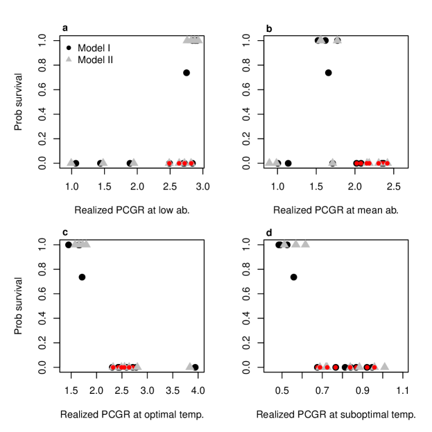
Figure S7: Probability of survival in the absence of a seed bank, as a function of the realized per capita growth rates (PCGR) of each species in different conditions. We consider (a) mean temperature and low densities, i.e., temperature is set to 15°C and all species densities are 1 cell/L, or (b) mean temperature (15°C) and average densities, i.e., all species are at their simulated average density values; or (c) optimal temperature for each species and average densities, or (d) suboptimal temperatures (30°C) and average densities. Red points correspond to species which have a high growth rate at low density but still go extinct.

Extinction in the absence of the seed bank is mostly due to a narrow niche: extinct species are always specialists (Fig. 5), even though these species should be able to invade a typical environment (Fig. S7 a) and tend to be less regulated than surviving species (Fig. S7 c, d).

S8 Absence of a storage effect in the model

The first step of our model (eq. 1 and 3 in main text) describes the increase in abundance of coastal and oceanic populations due to both environmental fluctuations and interactions with other organisms. The formula may be interpreted by certain readers as already including a storage effect, as shown by Miller & Klausmeier (2017) for a similar continuous-time model, or due to its apparent similarity to the model of Chesson (2003) in discrete time. We show below why the results of the cited analyses do not apply here and that the intra-compartment growth in discrete-time model does not lead to a storage effect.

The storage effect requires three elements: (a) a positive covariance between good environmental conditions and competition, (b) species-specific environmental responses and (c) subadditivity of environmental and competitive effects on the growth rate (Chesson, 2003). Condition (a) is met as covariance may be created by temporally correlated fluctuations in the environmental signal (Schreiber, 2021). Condition (b) is also met, as shown in Figure S3. Condition (c), however, is not met. Subadditivity of environmental and competitive effects can be mathematically expressed as $\frac{\partial}{\partial E}\left(\frac{\partial g}{\partial C}\right)<0$ where $g$ is the growth rate, and $E$ and $C$ are the effects of the environment and competition on the growth rate respectively.

In model I, the growth rate of a population is defined by the following equation:

$$N_{t+1,i}=\frac{\exp(r_{i}(T))N_{t,i}}{1+\sum_{j}\alpha_{ij}N_{t,j}}-lN_{t,i}$$

Here $E_{i}(t)=\exp(r_{i}(T))$ and $C_{i}(t)=1+\sum_{j}\alpha_{ij}N_{t,j}$. Therefore,

$$\begin{array}[]{ccc}g_{i}&=&\log\left(\frac{N_{t+1,i}}{N_{i}}\right)\\ &=&\log\left(\frac{\exp(r_{i}(T))}{1+\sum_{j}\alpha_{ij}N_{t,j}}-l\right)\\ &=&\log\left(\frac{E}{C}-l\right)\end{array}$$

Miller & Klausmeier (2017) consider instead a per capita growth rate (fitness) in continuous time $\frac{1}{N_{i}}\frac{dN_{i}}{dt}$.

While the discrete-time formula is at first sight very similar to the one in Chesson (2003), we wish to draw the reader’s attention to the fact that, contrary to Chesson (2003), interaction strengths do not depend on environmental effects, nor are they linearly correlated.

If we take derivatives with regards to competition effect $C$:

$$\begin{array}[]{ccc}\frac{\partial g}{\partial C}&=&-\frac{1}{C^{2}}\frac{E}{\frac{E}{C}-l}\\ &=&-\frac{E}{CE-lC}\end{array}$$

Finally, we take a derivative with respect to $E$:

$$\begin{array}[]{ccc}\frac{\partial}{\partial E}\left(\frac{\partial g}{\partial C}\right)&=&-\frac{CE-lC-EC}{(CE-lC)^{2}}\\ &=&\frac{lC}{(CE-lC)^{2}}\end{array}$$

As $C=1+\sum_{j}\alpha_{ij}N_{t,j}$ in the first model, or $C=1+\sum_{j\in\mathbb{C}}\frac{a_{C}N_{t,j,c/o}}{H_{ij}+N_{t,j,c/o}}+\sum_{j\in\mathbb{F}}\frac{a_{F}N_{t,j,c/o}}{H_{ij}+N_{t,j,c/o}}$ in the second model, which is never negative and always above 1, we always have $\frac{\partial}{\partial E}\left(\frac{\partial g}{\partial C}\right)>0$. There is no buffered growth in the effective growth rate itself, and therefore no storage effect in the coastal or oceanic compartment dynamics.

Now we highlight a more delicate point, in models that include the seed bank compartment. The storage effect could also be due to the presence of the seed bank, whose exchanges with other compartments are described in the second step of the model (eq. 4 in main text). The presence of a seed bank is indeed often associated with a storage effect maintaining coexistence (Angert et al., 2009), even though models show that this association is not systematic (Aikio et al., 2002). However, for the storage effect to happen due to the seed bank, theory currently highlights that environmental variations have to affect the recruitment rate, i.e. in our case, the germination and resuspension rates (Chesson, 2003). In our model, neither environmental nor competition effects affect the exchanges with the seed bank: the sinking and germination/resuspension rates are fixed and independent from both past and current environmental conditions. The storage effect is therefore unlikely to happen in our model. A thorough analysis of the storage effect based on simulations, as described by Ellner et al. (2016), would however be needed to conclude with complete certainty, as the presence of three distinct compartments may create non-obvious non-addivities or non-linearities.

References

- Aikio et al. (2002) Aikio, S., Ranta, E., Kaitala, V. & Lundberg, P. (2002). Seed bank in annuals: Competition between banker and non-banker morphs. Journal of Theoretical Biology, 217, 341–349.
- Anderson et al. (2005) Anderson, D.M., Stock, C.A., Keafer, B.A., Bronzino Nelson, A., Thompson, B., McGillicuddy, D.J., Keller, M., Matrai, P.A. & Martin, J. (2005). Alexandrium fundyense cyst dynamics in the Gulf of Maine. Deep Sea Research Part II: Topical Studies in Oceanography, 52, 2522–2542.
- Angert et al. (2009) Angert, A.L., Huxman, T.E., Chesson, P. & Venable, D.L. (2009). Functional tradeoffs determine species coexistence via the storage effect. PNAS, 106, 11641–11645.
- Ascione Kenov et al. (2015) Ascione Kenov, I., Muttin, F., Campbell, R., Fernandes, R., Campuzano, F., Machado, F., Franz, G. & Neves, R. (2015). Water fluxes and renewal rates at Pertuis d’Antioche/Marennes-Oléron Bay, France. Estuarine, Coastal and Shelf Science, 167, 32–44.
- Azanza et al. (2018) Azanza, R.V., Brosnahan, M.L., Anderson, D.M., Hense, I. & Montresor, M. (2018). The role of life cycle characteristics in harmful algal bloom dynamics. In: Global Ecology and Oceanography of Harmful Algal Blooms (eds. Glibert, P.M., Berdalet, E., Burford, M.A., Pitcher, G.C. & Zhou, M.). Springer International Publishing, Cham, vol. 232, pp. 133–161.
- Barraquand et al. (2018) Barraquand, F., Picoche, C., Maurer, D., Carassou, L. & Auby, I. (2018). Coastal phytoplankton community dynamics and coexistence driven by intragroup density-dependence, light and hydrodynamics. Oikos, 127, 1834–1852.
- Batifoulier et al. (2013) Batifoulier, F., Lazure, P., Velo-Suarez, L., Maurer, D., Bonneton, P., Charria, G., Dupuy, C. & Gentien, P. (2013). Distribution of Dinophysis species in the Bay of Biscay and possible transport pathways to Arcachon Bay. Journal of Marine Systems, 109-110, S273–S283.
- Bissinger et al. (2008) Bissinger, J., Montagnes, D., Harples, J. & Atkinson, D. (2008). Predicting marine phytoplankton maximum growth rates from temperature: Improving on the Eppley curve using quantile regression. Limnology and Oceanography, 53, 487–493.
- Boucher et al. (2020) Boucher, O. et al. (2020). Presentation and evaluation of the IPSL-CM6A-LR Climate Model. Journal of Advances in Modeling Earth Systems, 12.
- Cáceres (1997) Cáceres, C.E. (1997). Temporal variation, dormancy, and coexistence: A field test of the storage effect. Proceedings of the National Academy of Sciences, 94, 9171–9175.
- Chesson (2000) Chesson, P. (2000). Mechanisms of maintenance of species diversity. Annual review of Ecology and Systematics, pp. 343–366.
- Chesson (2003) Chesson, P. (2003). Quantifying and testing coexistence mechanisms arising from recruitment fluctuations. Theoretical population biology, 64, 345–357.
- Chesson (2018) Chesson, P. (2018). Updates on mechanisms of maintenance of species diversity. Journal of Ecology, 106, 1773–1794.
- Chesson & Huntly (1988) Chesson, P. & Huntly, N. (1988). Community consequences of life-history traits in a variable environment. Annales Zoologici Fennici, 25, 5–16.
- Chu & Adler (2015) Chu, C. & Adler, P.B. (2015). Large niche differences emerge at the recruitment stage to stabilize grassland coexistence. Ecological Monographs, 85, 373–392.
- Comita et al. (2010) Comita, L.S., Muller-Landau, H.C., Aguilar, S. & Hubbell, S.P. (2010). Asymmetric density dependence shapes species abundances in a tropical tree community. Science, 329, 330–332.
- Cushing et al. (2004) Cushing, J.M., Levarge, S., Chitnis, N. & Henson, S.M. (2004). Some discrete competition models and the competitive exclusion principle. Journal of difference Equations and Applications, 10, 1139–1151.
- Edwards et al. (2015) Edwards, K., Thomas, M., Klausmeier, C. & Litchman, E. (2015). Light and growth in marine phytoplankton: allometric, taxonomic, and environmental variation. Limnology and Oceanography, 60, 540–552.
- Edwards et al. (2016) Edwards, K., Thomas, M., Klausmeier, C. & Litchman, E. (2016). Phytoplankton growth and the interaction of light and temperature: A synthesis at the species and community level. Limnology and Oceanography, 61, 1232–1244.
- Eilertsen & Wyatt (2000) Eilertsen, H. & Wyatt, T. (2000). Phytoplankton models and life history strategies. South African Journal of Marine Science, 22, 323–337.
- Ellegaard & Ribeiro (2018) Ellegaard, M. & Ribeiro, S. (2018). The long-term persistence of phytoplankton resting stages in aquatic ‘seed banks’. Biological Reviews, 93, 166–183.
- Ellner (1987) Ellner, S. (1987). Alternate plant life history strategies and coexistence in randomly varying environments. Vegetatio, 69, 199–208.
- Ellner et al. (2016) Ellner, S., Snyder, R. & Adler, P. (2016). How to quantify the temporal storage effect using simulations instead of math. Ecology Letters, 19, 1333–1342.
- Eppley (1972) Eppley, R. (1972). Temperature and phytoplankton growth in the sea. Fishery Bulletin, 70, 1063–1085.
- Estrada et al. (2010) Estrada, M., Solé, J., Anglès, S. & Garcés, E. (2010). The role of resting cysts in Alexandrium minutum population dynamics. Deep Sea Research Part II: Topical Studies in Oceanography, 57, 308–321.
- Field et al. (1998) Field, C.B., Behrenfeld, M.J., Randerson, J.T. & Falkowski, P. (1998). Primary production of the biosphere: integrating terrestrial and oceanic components. science, 281, 237–240.
- Fox (2013) Fox, J.W. (2013). The intermediate disturbance hypothesis should be abandoned. Trends in Ecology & Evolution, 28, 86–92.
- Fransz & Verhagen (1985) Fransz, H. & Verhagen, J. (1985). Modelling research on the production cycle of phytoplankton in the Southern Bight of the North Sea in relation to riverborne nutrient loads. Netherlands Journal of Sea Research, 19, 241–250.
- Fujiwara et al. (2011) Fujiwara, M., Pfeiffer, G., Boggess, M., Day, S. & Walton, J. (2011). Coexistence of competing stage-structured populations. Scientific Reports, 1.
- Guittar et al. (2020) Guittar, J., Goldberg, D., Klanderud, K., Berge, A., Boixaderas, M.R., Meineri, E., Töpper, J. & Vandvik, V. (2020). Quantifying the roles of seed dispersal, filtering, and climate on regional patterns of grassland biodiversity. Ecology, 101, e03061.
- Hellweger et al. (2008) Hellweger, F.L., Kravchuk, E.S., Novotny, V. & Gladyshev, M.I. (2008). Agent-based modeling of the complex life cycle of a cyanobacterium (Anabaena) in a shallow reservoir. Limnology and Oceanography, 53, 1227–1241.
- Hense & Beckmann (2006) Hense, I. & Beckmann, A. (2006). Towards a model of cyanobacteria life cycle-effects of growing and resting stages on bloom formation of N2-fixing species. Ecological Modelling, 195, 205–218.
- Huang et al. (2016) Huang, Z., Liu, S., Bradford, K.J., Huxman, T.E. & Venable, D.L. (2016). The contribution of germination functional traits to population dynamics of a desert plant community. Ecology, 97, 250–261.
- Hutchinson (1961) Hutchinson, G.E. (1961). The paradox of the plankton. The American Naturalist, 95, 137–145.
- Jabot & Pottier (2017) Jabot, F. & Pottier, J. (2017). Macroecology of seed banks: The role of biogeography, environmental stochasticity and sampling. Global Ecology and Biogeography, 26, 1247–1257.
- Jewson et al. (1981) Jewson, D.H., Rippey, B.H. & Gilmore, W.K. (1981). Loss rates from sedimentation, parasitism, and grazing during the growth, nutrient limitation, and dormancy of a diatom crop. Limnology and Oceanography, 26, 1045–1056.
- Jones & Lennon (2010) Jones, S.E. & Lennon, J.T. (2010). Dormancy contributes to the maintenance of microbial diversity. PNAS, 107, 5881–5886.
- Kowe et al. (1998) Kowe, R., Skidmore, R., Whitton, B. & Pinder, A. (1998). Modelling phytoplankton dynamics in the River Swale, an upland river in NE England. Science of The Total Environment, 210, 535–546.
- Le Pape et al. (1999) Le Pape, O., Jean, F. & Ménesguen, A. (1999). Pelagic and benthic trophic chain coupling in a semi-enclosed coastal system, the Bay of Brest (France): a modelling approach. Marine Ecology Progress Series, 189, 135–147.
- Lee et al. (2018) Lee, S., Hofmeister, R. & Hense, I. (2018). The role of life cycle processes on phytoplankton spring bloom composition: a modelling study applied to the Gulf of Finland. Journal of Marine Systems, 178, 75–85.
- Levine & Rees (2004) Levine, J.M. & Rees, M. (2004). Effects of temporal variability on rare plant persistence in annual systems. The American Naturalist, 164, 350–363.
- Li et al. (2000) Li, M., Gargett, A. & Denman, K. (2000). What determines seasonal and interannual variability of phytoplankton and zooplankton in strongly estuarine systems? Estuarine, Coastal and Shelf Science, 50, 467–488.
- Locey (2010) Locey, K.J. (2010). Synthesizing traditional biogeography with microbial ecology: the importance of dormancy. Journal of Biogeography, 37, 1835–1841.
- Marcus & Boero (1998) Marcus, N. & Boero, F. (1998). Minireview: The importance of benthic-pelagic coupling and the forgotten role of life cycles in coastal aquatic systems. Limnology and Oceanography, 43, 763–768.
- Margalef (1978) Margalef, R. (1978). Life-forms of phytoplankton as survival alternatives in an unstable environment. Oceanologica acta, 1, 493–509.
- Martorell & Freckleton (2014) Martorell, C. & Freckleton, R.P. (2014). Testing the roles of competition, facilitation and stochasticity on community structure in a species-rich assemblage. Journal of Ecology, 102, 74–85.
- May (1981) May, R.M. (1981). Theoretical Ecology: Principles and Applications. Oxford University Press UK.
- McGillicuddy et al. (2005) McGillicuddy, D., Anderson, D., Lynch, D. & Townsend, D. (2005). Mechanisms regulating large-scale seasonal fluctuations in Alexandrium fundyense populations in the Gulf of Maine: Results from a physical-biological model. Deep Sea Research Part II: Topical Studies in Oceanography, 52, 2698–2714.
- McQuoid et al. (2002) McQuoid, M.R., Godhe, A. & Nordberg, K. (2002). Viability of phytoplankton resting stages in the sediments of a coastal Swedish fjord. European Journal Phycology, 37, 191–201.
- McQuoid & Hobson (1996) McQuoid, M.R. & Hobson, L.A. (1996). Diatom Resting Stages. Journal of Phycology, 32, 889–902.