Volumetric Objectives for Multi-Robot Exploration of Three-Dimensional Environments

Abstract

Volumetric objectives for exploration and perception tasks seek to capture a sense of value (or reward) for hypothetical observations at one or more camera views for robots operating in unknown environments. For example, a volumetric objective may reward robots proportionally to the expected volume of unknown space to be observed. We identify connections between existing information-theoretic and coverage objectives in terms of expected coverage, particularly that mutual information without noise is a special case of expected coverage. Likewise, we provide the first comparison, of which we are aware, between information-based approximations and coverage objectives for exploration, and we find, perhaps surprisingly, that coverage objectives can significantly outperform information-based objectives in practice. Additionally, the analysis for information and coverage objectives demonstrates that Randomized Sequential Partitions—a method for efficient distributed sensor planning—applies for both classes of objectives, and we provide simulation results in a variety of environments for as many as 32 robots.

I Introduction

Efficient exploration of unstructured three-dimensional environments can enable mapping of caves [1] and assistance in search and rescue [2] and is key to autonomy for aerial and ground robots. Planners for such robots seek to maximize various measures of reward for future camera views such as the volume of unknown space that the robots will observe. However, when the environment geometry is unknown, there is uncertainty in what the robots will observe and, in turn, how to assign rewards to as-yet unknown observations.

Methods for assigning volumetric rewards can be divided roughly into two groups: coverage-like and information-theoretic methods. Coverage methods compute rewards for observations given an assumed realization of the environment [3, 4, 5, 6]. While these approaches are simple the rewards they compute may not be representative of the actual observations. Alternatively, information-theoretic methods seek to compute reward (mutual information) given a distribution over environments via Bayesian priors [7, 8, 9, 10, 11]. However, information-theoretic methods are limited: all assume that cells in the map are independent; and, while rewards for depth observations along individual rays are accurate, rewards for multiple camera views are approximate [8]. This work relates these two families via connections to expected coverage, and our results, the first we are aware of comparing these two classes, suggest that coverage objectives may outperform existing information-theoretic methods in practice.

The same connections between mutual information and coverage also enable efficient distributed sensor planning. Many multi-robot sensing problems can be solved efficiently via greedy sequential planning methods for certain submodular objectives [12, 13, 14, 15]. However, these algorithms require robots to plan sequentially which causes planning time to increase with the size of the team and prevents designers from taking advantage of parallel computation. Some recent works study similar greedy planners where some robots can plan in parallel [16, 17, 18, 19, 20, 21]. However, many of these works provide suboptimality guarantees that degrade with increasing numbers of robots [19, 20, 21]. Now, while our earlier work on distributed exploration did not provide a-priori guarantees on solution quality [16], our recent work on planning via Randomized Sequential Partitions (RSP) provides guarantees on suboptimality that depend on an amount of inter-robot redundancy and for a slightly narrower class of objectives [18, 17]. The analysis in this paper demonstrates that these suboptimality guarantees are also applicable to exploration, for both mutual information and coverage objectives. Further, the results evaluate a variety of environments and numbers of robots and demonstrate that planning via RSP improves solution quality compared to more myopic planners while running with fewer steps than existing sequential methods.

Additionally, we note that an earlier (and slightly longer) version of this work appears in [18, Chapter 7].

II Background on submodular maximization

This work applies methods for maximizing submodular set functions to solve multi-robot receding-horizon sensor planning problems. Consider a collection of finite spaces of actions (or trajectories) ${\mathscr{B}}_{1},\ldots,{\mathscr{B}}_{{n_{\mathrm{r}}}}$ called blocks available to a team of ${{n_{\mathrm{r}}}}$ robots. The set of all of these actions ${\mathscr{U}}=\bigcup_{r\in\{1,\ldots,{{n_{\mathrm{r}}}}\}}{\mathscr{B}}_{r}$ is the ground set, and, while planning, each robot can select one action from its set of actions. Further, the set of complete and partial assignments ${\mathscr{I}}=\{I\subseteq{\mathscr{U}}\mid 1\geq|I\cap{\mathscr{B}}_{r}|\}$ forms a simple partition matroid [22, Sec. 39.4].

Then, a set function $g:2^{\mathscr{U}}\rightarrow$ maps a collection of such actions to a scalar such as to quantify sensor coverage or information gain. We treat unions implicitly so that $g(A,B)=g(A\cup B)$ for $A,B\subseteq{\mathscr{U}}$ and automatically wrap elements of subsets in sets so $g(x)=g(\{x\})$ for $x\in{\mathscr{U}}$.

Monotonicity conditions are important to many works that seek maximize set functions [23, 12], and many sensing objectives are known to have two such monotonicity conditions: monotonicity and submodularity [24]. Foldes and Hammer [25] defined a sequence of such monotonicity conditions. If a function is monotonically increasing, then for any $X\subseteq{\mathscr{U}}$ and $x\in{\mathscr{U}}\setminus X$ marginal gains are always positive

$$g(x|X)\geq 0$$ (1)

where $g(x|X)=g(x,X)-g(X)$, and this forms the 1-increasing condition [25]. Further, submodularity states that marginal gains decrease in the presence of a growing set of prior selections which forms the 2-decreasing condition. Specifically, given $A\!\subseteq\!B\subseteq\!{\mathscr{U}}$ and $x\!\in\!{\mathscr{U}}\!\setminus\!B$ submodularity states that

$$g(x|A)-g(x|B)\leq 0.$$ (2)

The coverage and mutual information objectives we study are known to be monotonic, submodular and normalized ($g(\emptyset)=0$). Additionally, set functions may also be 3-increasing which is useful for modeling redundancy between pairs of actions for efficient distributed planning [18, 17]. While weighted coverage objectives are 3-increasing, submodular mutual information objectives may not satisfy this requirement [17]. We then seek to determine whether or not mutual information objectives specific to exploration are 3-increasing as well.

III Minimum time exploration problem

Consider a team of robots ${\mathcal{R}}=\{1,\ldots,{n_{\mathrm{r}}}\}$ mapping a discretized environment $E=[c_{1},\ldots,c_{{n_{\mathrm{m}}}}]$ consisting of cells ${\mathcal{C}}=\{1,\ldots,{n_{\mathrm{m}}}\}$ that are each either free ($\bm{0}$) or occupied ($\bm{1}$) ($c_{i}\in\{0,1\}$), according to a probability distribution $\mathcal{E}_{\text{dist}}$. Each robot $r\in{\mathcal{R}}$ moves about with states $\mathbf{x}_{t,r}\in^{3}$ at each discrete time $t$ according to the dynamics

$$\mathbf{x}_{t,r} =f(\mathbf{x}_{t-1,r},u_{t,r})$$ (3)

where $u_{t,r}\in\mathcal{U}$ belongs to a finite set of control inputs. Robots must also remain in free space which induces the constraint that they remain in a safe set

$$\mathbf{x}_{t,r}\in\mathcal{X}_{\text{safe}}(E).$$ (4)

As they move about, the robots observe the environment with depth cameras. Assuming measurements are deterministic, without noise, robots can infer definitively that cells in the path of each ray are free up to the first occupied cell or the maximum range. Thus, when robots obtain observations from their depth cameras they can infer the occupancy of the set of cells ${F^{\mathrm{cam}}}(\mathbf{x},E)\subseteq{\mathcal{C}}$ which have occupancy values

$$\mathbf{y}_{t,r} =h(\mathbf{x}_{t,r},E)=\{(i,c_{i}):i\in{F^{\mathrm{cam}}}(\mathbf{x},E)\}.$$ (5)

The robots seek to observe as much of the environment as possible in terms of environment coverage:

$$J(\mathbf{X}_{1:t},\mathbf{Y}_{1:t})=\left|\bigcup\nolimits_{t^{\prime}\in\{1,\ldots,t\},r\in{\mathcal{R}}}{F^{\mathrm{cam}}}(\mathbf{x}_{t^{\prime},r},E)\right|.$$ (6)

Specifically, we seek to minimize time to reach a threshold on environment coverage, completing the exploration task.

IV Planning for exploration

Robots explore via receding-horizon planning and collectively maximize an objective $g$ over an $L$-step horizon

$$\max_{u^{\prime}_{1:L,1:{n_{\mathrm{r}}}}}~{} g(\mathbf{X}_{t:t+L,1:{n_{\mathrm{r}}}})$$

$$\mathrm{s.t.}~{} \mathbf{x}_{t+l,r}\in\mathcal{X}_{\text{safe}}(\mathbf{Y}_{1:t})$$

$$\mathbf{x}_{t+l,r}=f(\mathbf{x}_{t+l,r},u^{\prime}_{l,r})$$

$$\mathbf{y}_{t+l,r}=h(\mathbf{x}_{t+l,r},E)$$

$$\mbox{for all }l\in\{1\ldots L\}\mbox{ and }r\in{\mathcal{R}},$$ (7)

where $\mathcal{X}_{\text{safe}}(\mathbf{Y}_{1:t})$ refers to the set of states known to be safe given available observations (unlike (4) which refers to the complete set of safe states). Robots then execute the first control actions in the sequences $u^{\prime}_{1,1:{n_{\mathrm{r}}}}$ and repeat.

Additionally, we can interpret $g$ as a set function and rewrite (7) as a submodular maximization problem with a simple partition matroid constraint [16, 14, 15]. From this perspective, the ground set consists of assignments of control actions to robots ${\mathscr{U}}={\mathcal{R}}\times\mathcal{U}^{L}$, and the blocks of the partition matroid are assignments ${\mathscr{B}}_{r}=\{r\}\!\times\mathcal{U}^{L}$ to robots $r\in{\mathcal{R}}$.

We propose an objective that consists of two components $g_{\text{view}}$ and $g_{\text{dist}}$ so that, given $X\subseteq{\mathscr{U}}$, then

$$g(X) =g_{\text{view}}(X)+\sum_{r\in{\mathcal{R}}}g_{\text{dist}}(X_{r}),$$ (8)

where $X_{r}={\mathscr{B}}_{r}\cap X$ is the assignment to robot $r\in{\mathcal{R}}$. The view (or volumetric) reward $g_{\text{view}}$ seeks to capture the value of observations from camera views over the planning horizon while the distance component $g_{\text{dist}}$ rewards moving toward regions of the environment—often beyond the planning horizon—where valuable observations can be obtained.

The distance reward is based on our prior work [26] and rewards robots for reducing the distance to the nearest view with value ($g_{\text{view}}$) above a given threshold. This can be thought of as an analogue of nearest frontier exploration [27] for three-dimensional environments. Note that $g$ will remain normalized ($g(\emptyset)=0$) and retain the monotonicity properties of $g_{\text{view}}$ given that $g_{\text{dist}}$ is non-negative and zero when trajectories are not assigned (due to $g_{\text{dist}}$ being additive).

IV-A Sequential greedy assignment for submodular maximization

Sequentially maximizing $g$ for each robot provides solutions to receding-horizon planning problems (7) within half of optimal if individual robots plan optimally [12] or nearly so if robots plan approximately [13] so long as objective is submodular, monotonic, and normalized. Specifically, robots obtain solutions $X^{\mathrm{g}}=\{x_{1}^{\mathrm{g}},\ldots,x_{{n_{\mathrm{r}}}}^{\mathrm{g}}\}$ by planning greedily in sequence, maximizing $g$ conditional on prior solutions:

$$x_{r}^{\mathrm{g}}\in\operatorname*{arg\,max}_{x\in{\mathscr{B}}_{r}}g(x|X^{\mathrm{g}}_{1:r-1}).$$ (9)

This approach is simple and relatively efficient given that obtaining optimal solutions is NP-Hard. However, distributed implementations are intractable for large teams of robots as planning time increases because robots must plan in sequence rather than in parallel.

IV-B Distributed planning via Randomized Sequential Partitions

If $g$ is also 3-increasing, planning with Randomized Sequential Partitions (RSP) can take advantage of parallel computation and guarantee solutions approaching the original bound of one-half, depending on a measure of redundancy between robots [17, 18].

RSP planners run in a fixed number of steps ${n_{\mathrm{d}}}$ that does not grow with the number of robots (${{n_{\mathrm{r}}}}$). Robots planning via RSP assign themselves independently and randomly to one of ${n_{\mathrm{d}}}$ sequential steps. Then, robots assigned to the same step plan in parallel and maximize $g$ conditional on decisions from prior planning steps. Additionally, while this work does not focus on implementation, readers may refer to Corah [18] for a distributed, time-synchronous implementation of RSP.

V Volumetric rewards

The volumetric reward $g_{\text{view}}$ seeks to capture the joint value of observations (camera views) in terms of the amount of unknown space that the robots will collectively observe. Ideally, $g_{\text{view}}$ would correspond directly to actual increments in environment coverage (6). Except, the environment $E$ is unknown and, in turn, so are future values of the environment coverage. To mitigate this issue, prior works predominantly either compute rewards given an assumed [3, 4, 5, 6] (or possibly learned) guess at the environment instantiation or else by approximating mutual information for observations given a Bayesian prior [8, 9, 7, 11] so far always assuming independent (Bernoulli) cell occupancy. The following discussion unifies and contrasts these two families of exploration rewards and demonstrates that both coverage and information-based rewards satisfy the requirements for RSP planning.

V-A Expected coverage

We will relate different exploration rewards in terms of expected coverage. Consider some assumed distribution over possible environments $\mathcal{E}_{\text{dist}}$ with the requirement that any environment $\mathcal{E}_{\text{dist}}$ assigns non-zero probability $E^{\prime}\sim\mathcal{E}_{\text{dist}}$ must be consistent with observations up to the current time $\mathbf{Y}_{1:t}$ (although $\mathcal{E}_{\text{dist}}$ may assign non-zero probability to only a single realization). For convenience, define the set of future states that robots will visit while executing actions $X\subseteq{\mathscr{U}}$ as $\Phi(X)$. Given non-negative rewards for observing each cell $w_{\text{cell}}:{\mathcal{C}}\rightarrow_{\geq 0}$ the expected weighted coverage is

$$g_{\text{cov}}(X) ={{\mathds{E}}}_{E^{\prime}\sim\mathcal{E}_{\text{dist}}}\left[\sum_{i\in C_{\text{cov}}(X,E^{\prime})}w_{\text{cell}}(i)\right]$$ (10)

where $C_{\text{cov}}$ is the set of cells that the robots could observe:

$$C_{\text{cov}}(X,E^{\prime})=\bigcup\nolimits_{\mathbf{x}\in\Phi(X)}{F^{\mathrm{cam}}}(\mathbf{x},E^{\prime}).$$ (11)

We apply a weighting wcheme which provides a unit reward for each newly observed cell

$$w_{\text{new}}(i) =\begin{cases}0&i\in\bigcup\nolimits_{t^{\prime}\in\{1,\ldots,t\},r\in{\mathcal{R}}}{F^{\mathrm{cam}}}(\mathbf{x}_{t^{\prime},r},E)\\ 1&\text{otherwise (newly observed cells)}\end{cases}.$$ (12)

However, other weighting schemes are also relevant. For example, Yoder and Scherer [28] propose an objective for inspection tasks that encourages observing surfaces. Later, we will also find weighting cells by entropy produces a mutual information objective.

V-Aa Expected coverage retains monotonicity properties

The expected coverage (10) is normalized, monotonic, submodular, and 3-increasing because these conditions hold for weighted coverage [17, Theorem 5] and because the expectation over environments in (10) forms a convex combination which preserves monotonicity conditions (and being normalized) [25]. Likewise, suboptimality guarantees for RSP planning [17, 18] apply to receding-horizon planning for exploration with expected coverage.

V-B Noiseless mutual information for depth sensors

Most existing works on mutual information for occupancy mapping assume noisy measurements via either a general [7] noise model or simplified (often Gaussian) models [8, 10]. However, Zhang et al. [10] observed that the choice of information metric and noise model has little impact on performance in exploration experiments. Likewise, Henderson et al. [11] noted that sensor noise for modern lidar sensors and depth cameras is typically small compared to the maximum range. For these reasons, we assume that sensor noise is negligible for the purpose of evaluating mutual information for exploration and so ignore sensor noise in this work. Additionally, we assume that cell occupancy probabilities are independent according to the prior $\mathcal{E}_{\text{dist}}$ like previous works on mutual information for mapping [8, 7, 10].

The combination of cell independence and lack of sensor noise produces a special case of expected coverage:

Theorem 1 (Noiseless mutual information with independent cells is expected coverage).

The mutual information ${{\mathds{I}}}(E;\mathbf{Y}(X))$ between an environment $E$ with uncertain occupancy according to the distribution $\mathcal{E}_{\text{dist}}$ and hypothetical future observations $\mathbf{Y}(X)$ can be written as

$${{\mathds{I}}}(E;\mathbf{Y}(X)) ={{\mathds{E}}}_{E^{\prime}\sim\mathcal{E}_{\text{dist}}}\left[\sum\nolimits_{i\in C_{\text{cov}}(X,E^{\prime})}{{\mathds{H}}}(c_{i})\right].$$ (13)

where ${{\mathds{H}}}(c_{i})$ is the entropy of cell $c_{i}$, assuming:

1. Cell occupancy probabilities $\mathcal{E}_{\text{dist}}$ are independent, and

2. There is no sensor noise.

This expression (13) has the form of expected weighted coverage (10) and is therefore 3-increasing.

The proof is included in Appendix A. Theorem 1 produces insights into objective design and implies that suboptimality guarantees for RSP planning for 3-increasing functions apply to noiseless mutual information just as for expected coverage, even though mutual information is not 3-increasing in general [17].

V-C Design of volumetric objectives for exploration

Let us now expand on the prior two sections (Sec. V-A and Sec. V-B) which define volumetric exploration objectives and their properties and discuss the ramifications of the choice of a volumetric reward.

V-Ca Optimistic coverage

The definition of expected coverage also applies to degenerate priors over environments. Optimistic coverage is an expected coverage objective that optimistically assumes that unobserved space is empty and provides unit rewards (12) on unobserved cells; and numerous works on exploration develop similar objectives [3, 4]. Moreover, evaluation of optimistic coverage consists simply of counting newly observed cells. Thus, implementation is trivial even for joint observations by teams of robots.

V-Cb Occupancy priors for mutual information and optimism

Mapping applications and works exploration [7, 8, 10] frequently assume that unobserved cells are independent and occupied with a probability of 0.5. However, the environments that robots explore may predominantly consist of open space, and robots may actually observe more unknown space than they would otherwise predict. For this reason, our prior works [30, 31] select priors with relatively low occupancy probabilities. Similarly, Henderson [32] provides detailed discussion and illustrations that demonstrate how the occupancy prior can affect decisions.

A prior with a low occupancy probability assumes that unobserved cells are unoccupied like the optimistic coverage objective. As such, optimistic coverage is equivalent to mutual information in the limit after applying a scaling factor to (13) to normalize entropies of unobserved cells, assuming entropies of observed cells are zero. This is useful because optimistic coverage for multiple robots can be evaluated exactly while methods based on mutual information are approximate for multiple camera views [8, 11, 10].

VI Online bounds on solution quality

The 3-increasing condition establishes that RSP satisfies problem-dependent suboptimality guarantees for solving (7). Additionally, submodular objectives, such as the ones in this work, satisfy certain online bounds [33] which can provide much tighter guarantees for specific solutions [34, 35, 36]. Further, these bounds apply to any feasible solution which makes them suitable for comparison across different planners—even planners that do not satisfy specific guarantees.

While existing works study these online bounds in the context of cardinality-constrained problems, adapting these bounds to simple partition matroids is straightforward. Consider any—possibly incomplete—feasible solution $X\in{\mathscr{I}}$ to a receding-horizon planning problem as in Sec. IV and an optimal solution $X^{\star}$. The following holds, respectively, by monotonicity, submodularity, and greedy choice:

$$g(X^{\star}) \leq g(X,X^{\star})\leq g(X)+\sum_{x^{\star}\in X^{\star}}g(x^{\star}|X)$$

$$\leq g(X)+\sum_{r\in{\mathcal{R}}}\max_{x\in{\mathscr{B}}_{r}}g(x|X).$$ (14)

We apply two instances of the above bound. In the first, the online bound, $X$ is the full solution returned by the planner (assigning actions to all robots). Next, we call the case where $X=\emptyset$ (the empty set) the oblivious bound.

Figure 1 illustrates these bounds for a small set of exploration experiments. Observe that the tighter bound typically exceeds 70% which is significantly tighter than the a-priori bound of 1/2 for sequential planning. Later, we will use these bounds to characterize solution quality across trials with different planner configurations in lieu of comparison on common subproblems.

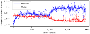
Figure 1: The above illustrates the online and oblivious bounds on suboptimality (solution value over bound) with five trials, sequential planning, and 16 robots with robots starting near the same position. The online bound is tighter early when robots are close together, and the oblivious bound becomes tighter later, as robots spread out. Note that the exploration process is nearly complete by 1000 robot-iterations, and evaluation is not exact due to approximation of (14) with MCTS. Shaded regions here and in the rest of the results delineate the standard error.

VII Experiment design

(a) 80 robot-iters.

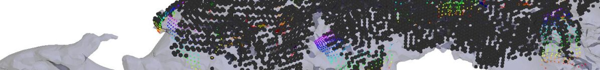
(b) 448 robot-iters.

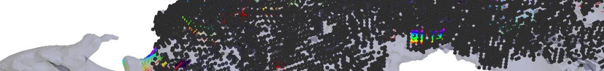
(c) 816 robot-iters.

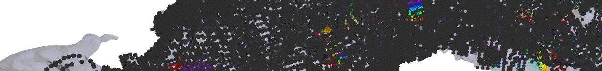
(d) 1184 robot-iters.

Figure 2: The images above visualize the process of exploration of the Skylight environment with 16 robots and RSP planning with ${n_{\mathrm{d}}}=6$. Additionally, a video providing examples of the exploration process is available at: %for␣each␣environment␣and␣number␣of␣robotshttps://youtu.be/B9j8LVIs384

This section describes the design of the exploration experiments. For intuition, Fig. 2 visualizes an example of the exploration process and provides a link to a video providing examples for all environments and numbers of robots.

VII-a Robot and sensor models

The robot dynamics are based on a kinematic quadcopter model. The set of control actions consists of $0.3\,$\mathrm{m}$$ translations in the cardinal directions with respect to the body frame as well as $\pi/2\,$\mathrm{rad}$$ yawing motions. Each robot obtains observations from a depth camera with a range of $2.4\,$\mathrm{m}$$, a resolution of $19\times 12$, and a field of view of $43.6$\mathrm{\SIUnitSymbolDegree}$\times 34.6$\mathrm{\SIUnitSymbolDegree}$$. Cameras face forward, oriented with the long axis vertical.

VII-b Single- and multi-robot planning

Robots plan by collectively solving receding-horizon planning problems (7) with optimistic coverage rewards (Sec. V-Ca). They plan to maximize the objective individually via Monte-Carlo tree search (MCTS) [37, 38, 39, 31] with 200 samples and collectively via specified methods for submodular maximization (Secs. IV-A and IV-B). The planners also discount rewards, treating each robot as having an independent probability of failure after each time-step. Although we do not provide detail, the discounts are compatible with the analysis of the objectives (Secs. V-A and V-B), and evaluation remains straightforward.

VII-c Environments and simulation scenarios

The simulation results evaluate performance across a variety of environments (listed in Table I). In each case, robots start with random yaw and slightly perturbed positions near a fixed starting location. We determined maximum coverage values and the lengths of the simulation trials (iterations per robot) through longer preliminary experiments with conservative parameters. Additionally, all maps use a $0.1\,$\mathrm{m}$$ discretization. So, a volume of $1\,${\mathrm{m}}^{3}$$ contains 1000 grid cells.

TABLE I: This table lists details of the test environments. While the bounding box volume provides the volume of a bounding box around the environment, the exploration volume lists the approximate maximum environment coverage volume for exploration.

Image	Name	14exBounding Box
Volume	12exExploration Volume
	Boxes	$216\,${\mathrm{m}}^{3}$$	$199\,${\mathrm{m}}^{3}$$
	Hallway-Boxes	$217\,${\mathrm{m}}^{3}$$	$202\,${\mathrm{m}}^{3}$$
	Plane-Boxes	$227\,${\mathrm{m}}^{3}$$	$212\,${\mathrm{m}}^{3}$$
	Empty	$500\,${\mathrm{m}}^{3}$$	$500\,${\mathrm{m}}^{3}$$
	Skylight	N/A	$220\,${\mathrm{m}}^{3}$$
	Office	$1300\,${\mathrm{m}}^{3}$$	$1180\,${\mathrm{m}}^{3}$$

VIII Results: Varying the distributed planner

TABLE II: Planner parameters for receding-horizon exploration. The myopic and sequential planners were tuned separately to maximize performance for 16 robots in the Boxes and Empty environments (Table. I). The parameter $c_{p}$ belongs to the MCTS planner [38] and is set to roughly half the typical value of the objective for a single robot. All RSP planners use parameters for sequential planning.

Planner	$c_{p}$	9exHorizon ($L$)	11exView Value
Threshold ($\epsilon_{\text{view}}$)	11exView Distance Factor ($\alpha$)	9exDiscount Factor
Sequential	1500	10	900	500	0.7
Myopic	1500	10	300	700	1.0

The first study evaluates the effect of the method of multi-robot coordination on exploration performance. The results compare sequential planning (Sec. IV-A), myopic planning (wherein robots plan via MCTS and ignore others’ decisions), and RSP with 1, 3, and 6 rounds (${n_{\mathrm{d}}}$). Parameters (see Table VIII) were selected separately for myopic and sequential planners with RSP inheriting parameters for sequential planning. We provide results for 10 trials per each configuration, varying planners, environments, and numbers of robots (4, 8, 16, and 32).

Figure 3 summarizes the exploration process for these simulations in terms of environment coverage (6). Although, there is not always much variation across planner configurations, these results also illustrate consistency in coverage rates, graceful degradation in efficiency (per-robot) with increasing numbers, and reliably complete exploration. The latter, reliable completion, is evident in convergence toward the maximum environment coverage and low variance toward the end of exploration trials.

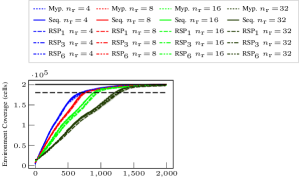
(e) Boxes

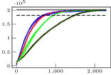
(f) Hallway-Boxes

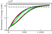
(g) Plane-Boxes

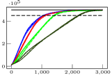
(h) Empty

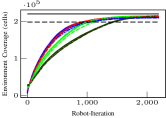
(i) Skylight

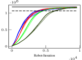
(j) Office

Figure 3: Environment coverage results for each environment with different planners. Black lines demarcate the maximum environment coverage for a given environment and dashed black lines mark a threshold at 90% of that value to represent task completion. Note, total coverage rates always increase with numbers of robots despite decrease in efficiency evident here.

VIII-A Online bounds on suboptimality

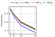
(a) Boxes

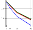
(b) Hallway-Boxes

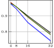
(c) Plane-Boxes

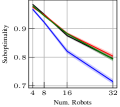
(d) Empty

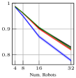
(e) Skylight

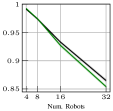
(f) Office

Figure 4: Lower bounds on suboptimality for receding-horizon planning for exploration in each environment. Plots provide mean values and standard error (w.r.t. the standard deviation of trial means) for data up to completion of the exploration task. These results demonstrate how the performance of RSP planning approaches that of sequential planning with increasing numbers of planning rounds from ${n_{\mathrm{d}}}=1$ to ${n_{\mathrm{d}}}=6$. We exclude the Myopic planner as the suboptimality bounds are not necessarily comparable to those of the other planners because the choice of parameters (Table VIII) changes the objective values. Instead, RSP₁ also plans myopically but has the same problem parameters as other planner configurations.

Figure 4 presents results on mean values of the lower bounds on suboptimality (the greater of the two bounds from Sec. VI). These plots demonstrate that the suboptimality of RSP planning approaches sequential planning (Sec. IV-A) with increasing numbers of planning rounds (${n_{\mathrm{d}}}$) as the performance bounds for these planners suggest [17]. Additionally, the actual suboptimality is consistently better than the worst case bound of 1/2 for sequential planning which is consistent with observations from related works [34, 35, 36]. Still, solutions for larger numbers of robots are more suboptimal for all planners and exhibit greater differences in suboptimality (reaching 8% for Empty). The decrease in these bounds with increasing numbers of robots is representative of robots operating in closer proximity and with greater overlap between observations over the planning horizon. As a whole, these results demonstrate RSP providing solution quality comparable to sequential planning with only 3 or 6 computation steps versus as many as 32 for sequential planning.

IX Results: Varying the objective

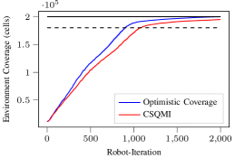
Figure 5: The above compares exploration with optimistic coverage and information-based CSQMI objectives [8] in terms of environment coverage in the Boxes environment. Black lines demarcate the maximum environment coverage, and a threshold at 90% to represent task completion.

Now, let us consider the effect of the choice of objective. This study, compares optimistic coverage (Sec. V-Ca) to an information-based objective, Cauchy-Schwarz quadratic mutual information (CSQMI) [8] with an occupancy prior of 0.125. Recall that optimistic coverage is equivalent to mutual information in the limit for small priors and is accurate for multiple rays and camera views. On the other hand, CSQMI and other information-based objectives [8, 7, 10, 11] can evaluate individual rays accurately but rely on approximations for collections of rays and views. Figure 5 plots the environment coverage for ten trials with sixteen robots in the Boxes environment. We compare performance in terms of time to complete the exploration task, defined as the time to reach 90% of the maximum exploration volume (see Tab. VIII).

Interestingly, robots planning with optimistic coverage explore the environment 16% faster than with CSQMI (averaging 890 robot-iterations versus 1067 respectively). While this result is limited in scope, the significant difference in performance suggests that accurate evaluation for multiple views may be more important than accurate evaluation of information gain for individual rays for robotic exploration.

X Conclusion and future work

This work has studied multi-robot exploration of three-dimensional environments from the perspective of design of objectives that quantify collections of camera views to reward observation of unknown space. Establishing that mutual information without noise is a special case of expected coverage enabled us to re-interpret coverage objectives as limiting cases of mutual information. Toward this end, simulation results found that employing a coverage-based objective improved completion time by 16% compared to a ray-based approximation of mutual information [8]. In future work, these results and our analysis may also produce improvements in approximation of mutual information based on expected coverage (see discussion in [18]).

The analysis also overcame an important challenge for distributed, receding-horizon planning for multi-robot exploration. By proving that mutual information without noise is expected coverage, we proved that this case satisfies suboptimality guarantees for distributed planning via Randomized Sequential Partitions (RSP) [17]. RSP runs with a fixed numbers of sequential steps rather than one per robot, unlike existing sequential methods [13, 12], so this is a significant result for distributed exploration. Additionally, the results demonstrated that distributed submodular maximization can provide consistent improvements in suboptimality on receding-horizon subproblems.

Appendix A Proof of Theorem 1

The following proves that noiseless mutual information with independent cells is 3-increasing by taking advantage of cell independence liberally to write mutual information in terms of the expected entropy of the cells that the robots will observe.

Proof.

We can write the mutual information between the environment $E$ and future observations $\mathbf{Y}(X)$ in terms of entropies:

$${{\mathds{I}}}(E;\mathbf{Y}(X)) ={{\mathds{H}}}(E)-{{\mathds{H}}}(E|\mathbf{Y}(X)).$$ (15)

The conditional entropy can then be rewritten in terms of the expected entropy given the direct observations of cell occupancy (5) associated with a hypothetical instantiation of the environment $E^{\prime}$ while abbreviating observed cells as $C^{\prime}=C_{\text{cov}}(X,E^{\prime})$:

$${{\mathds{I}}}(E;\mathbf{Y}(X)) ={{\mathds{H}}}(E)-{{\mathds{E}}}_{E^{\prime}\sim\mathcal{E}_{\text{dist}}}\left[{{\mathds{H}}}(E|E_{C^{\prime}}\!=\!E^{\prime}_{C^{\prime}})\right].$$ (16)

Then, observing that conditional entropy is simply the entropy of the cells that have not yet been observed $D^{\prime}={\mathcal{C}}\setminus C^{\prime}$, due to independence:

$${{\mathds{I}}}(E;\mathbf{Y}(X)) ={{\mathds{H}}}(E)-{{\mathds{E}}}_{E^{\prime}\sim\mathcal{E}_{\text{dist}}}\left[{{\mathds{H}}}(E_{D^{\prime}})\right].$$ (17)

Next, bringing the entropy of $E$ into the expectation does not change its value, and separating the independent observed and unobserved cells simplifies the expression:

$${{\mathds{I}}}(E;\mathbf{Y}(X)) ={{\mathds{E}}}_{E^{\prime}\sim\mathcal{E}_{\text{dist}}}\left[{{\mathds{H}}}(E_{C^{\prime}})+{{\mathds{H}}}(E_{D^{\prime}})-{{\mathds{H}}}(E_{D^{\prime}})\right].$$ (18)

$$={{\mathds{E}}}_{E^{\prime}\sim\mathcal{E}_{\text{dist}}}\left[{{\mathds{H}}}(E_{C^{\prime}})\right].$$ (19)

Finally, the joint entropy of the cells the robot will observe is the sum of their individual entropies

$${{\mathds{I}}}(E;\mathbf{Y}(X)) ={{\mathds{E}}}_{E^{\prime}\sim\mathcal{E}_{\text{dist}}}\left[\sum\nolimits_{i\in C_{\text{cov}}(X,E^{\prime})}{{\mathds{H}}}(c_{i})\right].$$ (20)

This expresses a weighted expected coverage objective (10) where the weight $w_{\text{cell}}(i)$ of each cell $i\in{\mathcal{C}}$ is equal to its entropy ${{\mathds{H}}}(c_{i})$. Observing that weighted expected coverage is 3-increasing (Sec. V-Aa) completes the proof. ∎

References

- Tabib et al. [2020] W. Tabib, K. Goel, J. Yao, C. Boirum, and N. Michael, “Autonomous cave surveying with an aerial robot,” arXiv preprint arXiv:2003.13883, 2020.
- Murphy et al. [2016] R. R. Murphy, S. Tadokoro, and A. Kleiner, “Disaster robotics,” Springer Handbook of Robotics, pp. 1577–1604, 2016.
- Simmons et al. [2000] R. Simmons, D. Apfelbaum, W. Burgard, D. Fox, M. Moors, S. Thrun, and H. Younes, “Coordination for multi-robot exploration and mapping,” in Assoc. for Adv. of Artif. Intell., 2000, pp. 852–858.
- Butzke and Likhachev [2011] J. Butzke and M. Likhachev, “Planning for multi-robot exploration with multiple objective utility functions,” in 2011 IEEE/RSJ International Conference on Intelligent Robots and Systems. IEEE, 2011, pp. 3254–3259.
- Delmerico et al. [2018] J. Delmerico, S. Isler, R. Sabzevari, and D. Scaramuzza, “A comparison of volumetric information gain metrics for active 3D object reconstruction,” Auton. Robots, vol. 42, no. 2, pp. 197–208, 2018.
- Bircher et al. [2018] A. Bircher, M. Kamel, K. Alexis, H. Oleynikova, and R. Siegwart, “Receding horizon path planning for 3D exploration and surface inspection,” Auton. Robots, vol. 42, no. 2, pp. 291–306, 2018.
- Julian et al. [2014] B. J. Julian, S. Karaman, and D. Rus, “On mutual information-based control of range sensing robots for mapping applications,” Intl. Journal of Robotics Research, vol. 33, no. 10, pp. 1357–1392, 2014.
- Charrow et al. [2015a] B. Charrow, S. Liu, N. Michael, and V. Kumar, “Information-theoretic mapping using Cauchy-Schwarz quadratic mutual information,” in Proc. of the IEEE Intl. Conf. on Robot. and Autom., Seattle, WA, May 2015.
- Charrow et al. [2015b] B. Charrow, G. Kahn, S. Patil, S. Liu, K. Goldberg, P. Abbeel, N. Michael, and V. Kumar, “Information-theoretic planning with trajectory optimization for dense 3D mapping,” in Proc. of Robot.: Sci. and Syst., Rome, Italy, Jul. 2015.
- Zhang et al. [2020] Z. Zhang, T. Henderson, S. Karaman, and V. Sze, “FSMI: Fast computation of shannon mutual information for information-theoretic mapping,” Intl. Journal of Robotics Research, 2020.
- Henderson et al. [2020] T. Henderson, V. Sze, and S. Karaman, “An efficient and continuous approach to information-theoretic exploration,” in Proc. of the IEEE Intl. Conf. on Robot. and Autom., May 2020.
- Fisher et al. [1978] M. L. Fisher, G. L. Nemhauser, and L. A. Wolsey, “An analysis of approximations for maximizing submodular set functions-II,” Polyhedral Combinatorics, vol. 8, pp. 73–87, 1978.
- Singh et al. [2009] A. Singh, A. Krause, C. Guestrin, and W. J. Kaiser, “Efficient informative sensing using multiple robots,” J. Artif. Intell. Res., vol. 34, pp. 707–755, 2009.
- Atanasov et al. [2015] N. A. Atanasov, J. Le Ny, K. Daniilidis, and G. J. Pappas, “Decentralized active information acquisition: Theory and application to multi-robot SLAM,” in Proc. of the IEEE Intl. Conf. on Robot. and Autom., Seattle, WA, May 2015.
- Schlotfeldt et al. [2018] B. Schlotfeldt, D. Thakur, N. Atanasov, V. Kumar, and G. J. Pappas, “Anytime planning for decentralized multi-robot active information gathering,” IEEE Robot. Autom. Letters, vol. 3766, no. c, pp. 1–8, 2018.
- Corah and Michael [2017] M. Corah and N. Michael, “Efficient online multi-robot exploration via distributed sequential greedy assignment,” in Proc. of Robot.: Sci. and Syst., Cambridge, MA, 2017.
- Corah and Michael [2018] ——, “Distributed submodular maximization on partition matroids for planning on large sensor networks,” in Proc. of the IEEE Conf. on Decision and Control, Miami, FL, Dec. 2018.
- Corah [2020] M. Corah, “Sensor planning for large numbers of robots,” Ph.D. dissertation, Carnegie Mellon University, 2020.
- Grimsman et al. [2018] D. Grimsman, M. S. Ali, J. P. Hespanha, and J. R. Marden, “The impact of information in greedy submodular maximization,” IEEE Transactions on Control of Network Systems, 2018.
- Gharesifard and Smith [2017] B. Gharesifard and S. L. Smith, “Distributed submodular maximization with limited information,” IEEE Trans. Control Netw. Syst., 2017, to appear.
- Sun et al. [2020] H. Sun, D. Grimsman, and J. R. Marden, “Distributed submodular maximization with parallel execution,” in Proc. of the Amer. Control Conf., Denver, CO, 2020.
- Schrijver [2003] A. Schrijver, Combinatorial optimization: polyhedra and efficiency. Springer Science & Business Media, 2003, vol. 24.
- Nemhauser and Wolsey [1978] G. L. Nemhauser and L. A. Wolsey, “Best algorithms for approximating the maximum of a submodular set function,” Mathematics of operations research, vol. 3, no. 3, pp. 177–188, 1978.
- Krause and Guestrin [2005] A. Krause and C. E. Guestrin, “Near-optimal nonmyopic value of information in graphical models,” in Proc. of the Conf. on Uncertainty in Artif. Intell., Edinburgh, Scotland, 2005.
- Foldes and Hammer [2005] S. Foldes and P. L. Hammer, “Submodularity, supermodularity, and higher-order monotonicities of pseudo-boolean functions,” Mathematics of Operations Research, vol. 30, no. 2, pp. 453–461, 2005.
- Corah et al. [2019] M. Corah, C. O’Meadhra, K. Goel, and N. Michael, “Communication-efficient planning and mapping for multi-robot exploration in large environments,” IEEE Robot. Autom. Letters, vol. 4, no. 2, pp. 1715–1721, 2019.
- Yamauchi [1997] B. Yamauchi, “A frontier-based approach for autonomous exploration,” in Proc. of the Intl. Sym. on Comput. Intell. in Robot. and Autom., Monterey, CA, Jul. 1997.
- Yoder and Scherer [2016] L. Yoder and S. Scherer, “Autonomous exploration for infrastructure modeling with a micro aerial vehicle,” in Field and Service Robotics. Springer, 2016, pp. 427–440.
- Cover and Thomas [2012] T. M. Cover and J. A. Thomas, Elements of Information Theory. New York, NY: John Wiley & Sons, 2012.
- Tabib et al. [2016] W. Tabib, M. Corah, N. Michael, and R. Whittaker, “Computationally efficient information-theoretic exploration of pits and caves,” in Proc. of the IEEE/RSJ Intl. Conf. on Intell. Robots and Syst., Daejeon, Korea, Oct. 2016.
- Corah and Michael [2019] M. Corah and N. Michael, “Distributed matroid-constrained submodular maximization for multi-robot exploration: theory and practice,” Auton. Robots, vol. 43, no. 2, pp. 485–501, 2019.
- Henderson [2019] T. Henderson, “A continuous approach to information-theoretic exploration with range sensors,” Master’s thesis, Massachusetts Institute of Technology, 2019.
- Minoux [1978] M. Minoux, “Accelerated greedy algorithms for maximizing submodular set functions,” in Optimization techniques. Springer, 1978, pp. 234–243.
- Leskovec et al. [2007] J. Leskovec, A. Krause, C. Guestrin, C. Faloutsos, J. VanBriesen, and N. Glance, “Cost-effective outbreak detection in networks,” in Proceedings of the 13th ACM SIGKDD international conference on Knowledge discovery and data mining, 2007, pp. 420–429.
- Golovin and Krause [2011] D. Golovin and A. Krause, “Adaptive submodularity: Theory and applications in active learning and stochastic optimization,” Journal of Artificial Intelligence Research, vol. 42, pp. 427–486, 2011.
- Krause et al. [2008] A. Krause, J. Leskovec, C. Guestrin, J. VanBriesen, and C. Faloutsos, “Efficient sensor placement optimization for securing large water distribution networks,” Journal of Water Resources Planning and Management, vol. 134, no. 6, pp. 516–526, 2008.
- Chaslot [2010] G. Chaslot, “Monte-Carlo tree search,” Ph.D. dissertation, Universiteit Maastricht, 2010.
- Browne et al. [2012] C. Browne, E. Powley, D. Whitehouse, S. Lucas, P. I. Cowling, P. Rohlfshagen, S. Tavener, D. Perez, S. Samothrakis, and S. Colton, “A survey of Monte Carlo tree search methods,” IEEE Trans. on Comput. Intell. and AI in Games, vol. 4, no. 1, pp. 1–43, 2012.
- Lauri and Ritala [2016] M. Lauri and R. Ritala, “Planning for robotic exploration based on forward simulation,” Robot. Auton. Syst., vol. 83, pp. 15–31, 2016.