Learn-to-Race: A Multimodal Control Environment for Autonomous Racing

Abstract

Existing research on autonomous driving primarily focuses on urban driving, which is insufficient for characterising the complex driving behaviour underlying high-speed racing. At the same time, existing racing simulation frameworks struggle in capturing realism, with respect to visual rendering, vehicular dynamics, and task objectives, inhibiting the transfer of learning agents to real-world contexts. We introduce a new environment, where agents Learn-to-Race (L2R) in simulated competition-style racing, using multimodal information—from virtual cameras to a comprehensive array of inertial measurement sensors. Our environment, which includes a simulator and an interfacing training framework, accurately models vehicle dynamics and racing conditions. In this paper, we release the Arrival simulator for autonomous racing. Next, we propose the L2R task with challenging metrics, inspired by learning-to-drive challenges, Formula-style racing, and multimodal trajectory prediction for autonomous driving. Additionally, we provide the L2R framework suite, facilitating simulated racing on high-precision models of real-world tracks. Finally, we provide an official L2R task dataset of expert demonstrations, as well as a series of baseline experiments and reference implementations. We make all code available: https://github.com/learn-to-race/l2r.

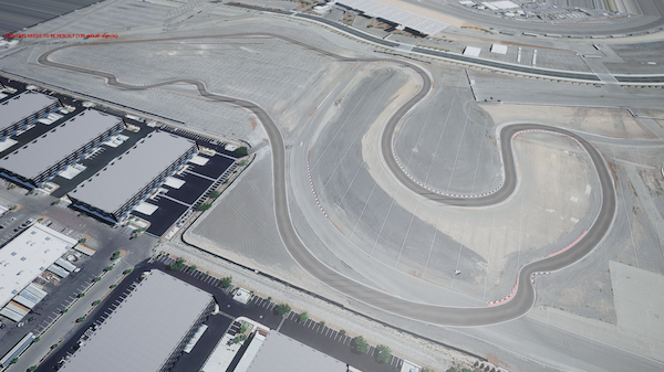
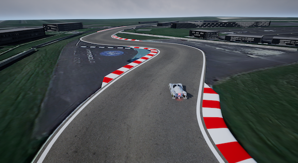
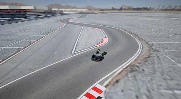
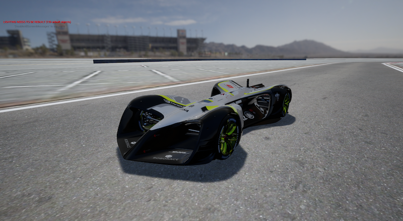
Figure 1: Learn-to-Race interfaces with a racing simulator, which features numerous real-world racetracks such as the Thruxton Circuit (top-left) and Las Vegas Motor Speedway (top-right). Simulated race cars (bottom) are empowered with learning agents, tasked with the challenge of learning to race for the fastest lap-times and best metrics.

1 Introduction

Progress in the field of autonomous driving relies on the existence of challenging tasks and well-defined evaluation metrics, which enable researchers to effectively assess and improve algorithms. Models developed in learning-to-drive settings continue to struggle with issues in sample-complexity, safety, and unseen generalisation, calling for more suitable benchmarks [9, 16, 28]. We hypothesise that high-fidelity simulation environments, together with well-defined metrics and evaluation procedures, are conducive to developing more sophisticated agents; and, in turn, such agents will be better-suited to real-world deployment.

Simulated autonomous racing exhibits task complexity on several factors: (i) agents must perform real-time decision making, requiring computationally-efficient policy updates as well as robustness to latency; (ii) agents must be able to deal with realistic vehicle and environmental dynamics (whereas agents in less-realistic environments have been able to achieve super-human performance); (iii) agents must leverage more informative intrinsic reward schemes that enable replication of human-like driving behaviour, e.g., trading off safety and performance; and (iv) agents must use offline demonstrations effectively, without overfitting, and must leverage interactions with the environment sample-efficiently. We highlight simulated racing (Figure 1) as an opportunity for developing learning strategies that are capable of meeting these stringent requirements.

In this work, we release the Arrival Autonomous Racing Simulator, which includes numerous interfaces for both simulated and real vehicle instrumentation. Furthermore, we introduce Learn-to-Race (L2R), a multimodal and continuous control environment for training and evaluating autonomous racing agents. Through the L2R environment, we simulate competition-style racetracks that are based off real-world counterparts, we provide mechanisms for fully-characterising realistic racing agents (e.g., flexible sensor placements, multimodal cameras, and various vehicle dynamics profiles), and we provide numerous tools for fine-grained agent evaluation (e.g., random and fixed spawn locations, custom racing map construction, and injection of external disturbances). Using these facilities, we enable research in problems that require agents to make safety-critical, sub-second decisions in dynamically unstable contexts, such as autonomous racing, real-time uncertainty analysis in highway driving, and trajectory forecasting. In this paper, we exemplify algorithm development and benchmarking of methods under learning from demonstrations, reinforcement learning, and model-predictive control.

Concretely, our contributions include: (i) the Arrival Autonomous Racing Simulator, which simulates high-fidelity competition-style tracks, vehicles, and various sensor signals; (ii) the Learn-to-Race (L2R) framework, a plug-and-play environment, which defines interfaces for various sensor modalities and provides an OpenAI-gym compliant training and testing environment for learning-based agents; (iii) an official L2R task and dataset with expert demonstrations, metrics, and reference evaluation procedures; and (iv) an academic release of the simulator, code for the L2R framework, and implementations of baseline agents to facilitate full reproducibility and extension.

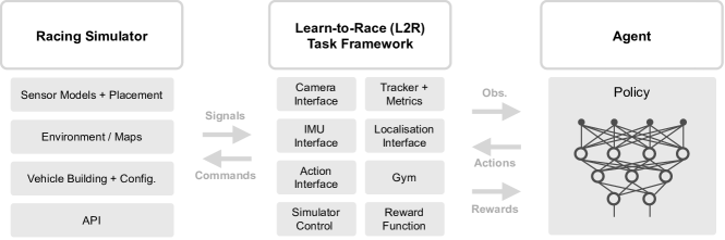
Figure 2: Learn-to-Race allows agents to interact with the racing simulator through a series of interfaces for observations, actions, and simulator control.

2 Related Work

2.1 Reinforcement Learning Environments

Research progress in the fields of Reinforcement Learning (RL), Planning, and Control has relied on various simulation environments, for benchmarking agent performance on game-playing and robot control tasks [32, 8, 33, 18, 30]. These tasks require sequential decision-making in order to complete objectives and are generally characterised by their state dimensionality, the nature of their action space (e.g., discrete or continuous), agent cardinality (i.e., single- or multi-agent), and by the capability of the underlying simulator in capturing real-world physical dynamics [18]. Whereas the vast majority of tasks offered by, e.g., the DeepMind Control Suite [32], OpenAI Gym [8], and the MuJoCo physics engine [33] have been solved—with agents often achieving superhuman performance—no existing environments focus on high-fidelity simulation of high-speed driving, in dynamically unstable contexts.

2.2 Simulation of Autonomous Driving

Urban driving. CARLA [14] is an open-source simulator for autonomous driving, wherein various tasks have been defined to challenge agents’ street-legal urban driving abilities. Duckietown [29, 10] provides a customisable platform for urban autonomous driving, as well as hardware support for miniature vehicles controlled via RaspberryPi’s. In this paper, we focus primarily on autonomous racing environments, which present challenges outside the conventional scope of urban and highway driving.

Track racing. In autonomous racing, agents must make sub-second decisions in regimes of unstable physical dynamics, wherein the ramifications of control actions can be amplified or suppressed, non-linearly, depending on vehicular and environmental state. CarRacing-v0, an OpenAI-gym environment [8], is a simple racing environment, which uses only bird’s-eye-view (BEV) observations. In [17], researchers trained agents to race in the video game Gran Turismo Sport, but have not yet released their environment. Moreover, instead of using sensory perception, agents were directly provided with privileged information, e.g., distance to obstacles and road boundaries. TORCS [3] is an open-source simulator and is used by the Simulated Car Racing Championship [27], despite its game-like qualities. As the goal of simulators should be to accurately model the dynamics of the real-world, we assert that the potential for model transfer from these frameworks remains limited.

2.3 Learning Paradigms

We discuss various learning paradigms that are enabled by the simulation of autonomous driving.

Simulation-to-real transfer. DeepRacer [5], developed by Amazon Web Services, provides an end-to-end framework for training and deploying 1/18th-scale autonomous racing cars. The Indy Autonomous Challenge [1] encourages institutions to create autonomous vehicle technology; participants are given the proprietary VRXPERIENCE driving simulator, which focuses more on optimising human-machine interactions within the vehicle, in the context of situational highway driving, which contrasts with our focus in this work on autonomous racing. Roborace [2] is the first international championship for full-size, real-world autonomous racing. Here, teams develop self-driving software and compete in challenges, using Roborace-owned vehicles. Roborace provides teams with proprietary software-in-the-loop (SIL) and hardware-in-the-loop (HIL) simulators, with a base driving stack. These simulators are predominately used for developing classical control methods, however, and do not include facilities for training learning-based agents [7, 22, 23, 31]. The authors obtained a podium finish at the Thruxton Circuit (UK), in the Season Beta Roborace competitions (2020-2021), and we now wish to enable new technologies through open-sourcing our autonomous racing research: to our knowledge, we publicly release the first environment that is specifically intended for simulating autonomous competition-style track racing and for transferring learning-based agents to the real world.

Safe and efficient learning. Imposing safety constraints in, e.g., RL algorithms, has become popular for the potential of reducing failures in simulation-to-real transfer settings and for enabling agent robustness to environmental stochasticity [20]. The goal is to embed safety guarantees in policies, without compromising their performance or sample-efficiency. While a few works consider detection and avoidance of unsafe states, in urban driving [13] and human-assistive robotics [19], no existing works focus on safe learning and control, for autonomous racing in dynamically unstable contexts. Popular Safe-RL benchmarks (e.g., OpenAI Safety Gym) lack realistic dynamics and they evaluate agents at much lower speeds; thus, the numerous limitations of existing methods cannot be studied comprehensively. We assert that the physical realism that L2R provides facilitates improvement of those underlying approaches.

3 Simulation Environment

3.1 Arrival Autonomous Racing Simulator

The Arrival simulator is a powerful tool for the development and testing of autonomous vehicles. It is based on Unreal Engine 4 and includes such features as: (i) a vehicle prototyping framework; (ii) full software-in-the-loop (SIL) simulation, to model all vehicle control devices; (iii) controller area network (CAN) bus interface; (iv) camera, inertial measurement unit (IMU), light detection and ranging (LiDAR), ultrasonic, and radar sensor models; (v) semantic segmentation; (vi) sensor placement and configuration facilities; (vii) V2V/V2I interface subsystem; (vii) dynamic racing scenario creation; (viii) race track generation from scanned datasets; (ix) support for full integration with the CARLA simulator [14]; and (x) an application programming interface (API), which is automatically generated based on C++ code analysis. Details in supplementary.

3.2 Learn-to-Race Environment

Learn-to-Race (L2R) is a multimodal control environment that provides a series of interfaces for an agent to interact with the racing simulator, including the capabilities to send control commands and make observations of the environment and vehicle state via different sensors (Figure 2). L2R is implemented as a Gym environment [8], enabling quick prototyping of control policies. While we release the L2R environment and task (Section 4) alongside the Arrival simulator, we note that other simulators may be used with L2R, including those provided by [2].

Agent-Simulator Interaction. At each step $t$, an agent selects an action $a_{t}$, based on its current observation $s_{t}$, using its policy $\pi_{\theta}$: $a_{t}\sim\pi_{\theta}(\cdot|s_{t})$. The control action from the agent is forwarded to the simulator as a UDP message. L2R receives updates from the simulator, i.e., images from the virtual camera and/or measurements from other vehicle sensors, through TCP and UDP socket connections. As in reality, update frequencies across the various sensor modalities are not equal, so L2R synchronizes observations by providing agents with the most recent data from each (Algorithm 1). The step method of the environment returns the new observation $s_{t+1}$, along with a calculated reward to the agent, $r_{t}=R(s_{t},a_{t},s_{t+1})$, and a Boolean terminal state flag. The reward function and evaluation metrics are defined in Section 4.3.

Algorithm 1 Agent-Simulator Interaction

1:function Sensor Thread

2:     $data\leftarrow$ Initial value

3:     function Get Data

4:         return $data$      

5:     while $not\>terminated$ do

6:         $data\leftarrow$ Receive Data      

7:

8:function Step($a_{t}$)

9:     Send $a_{t}$ as UDP message

10:     $s_{t+1}\leftarrow$ Get Data $\forall$ Sensor Threads

11:     $r_{t}\leftarrow R(s_{t},a_{t},s_{t+1})$

12:     $done\leftarrow$ IsTerminal($s_{t},s_{t+1}$)

13:     return $s_{t+1},\>r_{t},\>done$

Episodic control. The control interface communicates with the simulator to automatically setup and execute simulations in an episodic manner. L2R conveniently allows for training to be launched in one command, as all aspects of the racing simulator and learning environment are parameterised. A state is considered terminal if all laps are successfully completed, if at least 2 of the vehicle’s wheels go outside of the drivable area, or if progress is minimally insufficient. The episode begins by resetting the vehicle to a standing start position, at a parameterised location along with configured sensor interfaces and initialised reward function. Discrete steps are taken by the agent until one of the aforementioned episode termination criteria is met.

4 Task: Learn-to-Race

The Learn-to-Race (L2R) task tests an agent’s ability to execute the requisite behaviours for competition-style track racing, through multimodal perceptual input. In this section, we provide a task overview and describe task properties, dataset characteristics, and metrics.

4.1 Task Overview

L2R provides an OpenAI Gym [8] compliant learning environment, where researchers could flexibly select among the available sensor modalities. This early version of the environment enables single-agent racing on three racetracks (with custom track construction facility), modeled after their real-world counterparts. Included tracks are the Thruxton Circuit (Track01:Thruxton) and Anglesey National Circuit (Track02:Anglesey) from the United Kingdom, and the North Road Track at Las Vegas Motor Speedway (Track03:Vegas), located in the United States. Analogous to having separate town maps for training and testing in other simulation environments, e.g., CARLA [14], we use Track01 and Track02 for training and Track03 for testing. Consequently, we generate expert traces from the training tracks, for inclusion in our initial dataset release (see Section 4.2). Many avenues for research can be explored within L2R, including various learning paradigms, such as: (constrained) reinforcement learning, learning from demonstrations, multitask learning, transfer learning and domain adaptation, simulation-to-real transfer, fast decision-making, classical/neural hybrid modeling, etc. Regardless of the method chosen, agents’ multimodal perception capabilities—i.e., their ability to fuse and align sensory information—are of critical importance.

Table 1: Summary of the observation and continuous action spaces, for the Learn-to-Race task. When the simulator is initialised in vision-only mode, the observation space consists of just the images from the ego-vehicle’s front-facing camera. The additional observation data, all of which is realistically accessible on a real racing car, is available in multimodal mode. *Whereas gear is permitted as a controllable parameter, we do not use it in our experiments.

	Signal	Description	Dimension
Action	Acceleration	Command in [-1.0, 1.0]	$\mathbb{R}^{1}$
	Steering	Command in [-1.0, 1.0]	$\mathbb{R}^{1}$
	Gear	{park, drive, neutral, reverse}	—
Observation	Image	RGB image	$\mathbb{R}^{W\times H\times 3}$
	Steering	Observed steering direction	$\mathbb{R}^{1}$
	Gear	{park, drive, neutral, reverse}	—
	Mode	Vehicle mode	$\mathbb{R}^{1}$
	Velocity	In ENU coordinate ($m/s$)	$\mathbb{R}^{3}$
	Acceleration	In ENU coordinate ($m/s^{2}$)	$\mathbb{R}^{3}$
	Yaw, Pitch, Roll	Orientation of the car ($rad$)	$\mathbb{R}^{3}$
	Angular Velocity	Rate of change of the orientation ($rad/s$)	$\mathbb{R}^{3}$
	Location	Location of the vehicle center in ENU ($m$)	$\mathbb{R}^{3}$
	Wheel Rotational Speed	per wheel (RPM)	$\mathbb{R}^{4}$
	Braking	Brake pressure per wheel ($Pa$)	$\mathbb{R}^{4}$
	Torque	per wheel ($N\dot{m}$)	$\mathbb{R}^{4}$

4.2 Learn-to-Race Dataset

We generate a rich, multimodal dataset of expert demonstrations from training tracks, Track01:Thruxton and Track02:Anglesey, in order to facilitate pre-training of agents via, e.g., imitation learning (IL). The L2R dataset contains multi-sensory input at a 100-millisecond resolution, in both the observation and action spaces. Depending on the selected simulator perception mode, agents have access to one (vision-only mode) or all modalities (multimodal mode). See Table 1 for a complete list of available modalities. The action space is defined by continuous values for acceleration and steering, in the ranges $[-1.0,1.0]$, where negative acceleration values will decelerate the vehicle to a halted position. Note that Gear is a controllable action, but fixed to drive in all our experiments.

The expert demonstrations were collected using a model predictive controller (MPC) (Section 5), which follows the centerline of the race track at a pre-specified reference speed. This first version of the dataset contains 10,600 samples of each sensor and action dimension, for 9 complete laps around each track. Future version releases of L2R will include access to new simulated tracks (modeled after other real tracks, around the world) as well as expert traces generated from these additional tracks—across various weather conditions, in challenging multi-agent settings, and within dangerous obstacle-avoidance scenarios.

4.3 Task Metrics

The primary objective of the L2R task is to minimise the time taken for an agent to successfully complete racing laps, with additional requirements on the agent’s driving quality. We do not restrict the agent’s learning paradigms to, e.g., IL or RL; on the contrary, we can envision a wealth of combination strategies and other methods that are applicable to the task. While we do not include planning-only approaches as those that are consistent with the official L2R task, (i) we do encourage hybrid or model-based learning approaches; furthermore, (ii) we do encourage the simulator and the L2R interface to be used to further research in these areas, more generally. Agnostic to the learning paradigm used, and inspired by concepts from high-speed driving, robot navigation [18], and trajectory forecasting [28], we define the core modalities, metrics, and objectives that shall be used to train L2R agents and assess their performance. We summarise agents’ action and observation spaces in Table 1 and the official L2R task metrics in Table 2.

We define the successful completion of an episode in the L2R task to be 3 completed laps, from a standing start; Episode Completion Percentage (ECP) measures the amount of the episode completed, and Episode Duration (ED) measures the minimum amount of time that the agent took to progress to its furthest extent, through the episode. We define Average Adjusted Track Speed (AATS) as a metric that measures the average speed of the agent, across all three laps of the episode. Metrics may also include adjustments for environmental factors, such as wheel slippage and weather effects as the task matures. Average Displacement Error (ADE), a common metric in trajectory forecasting [28], measures the agent’s average deviation from a reference path—in this case, the centerline of the track. Trajectory Admissibility (TrA) is the dimensionless metric $\alpha$, defined in Equation 1, where $t_{e}$ is the duration of the episode and $t_{u}$ is the cumulative time spent driving unsafely with exactly one wheel outside of the drivable area.

$$\alpha=1-\sqrt{\frac{t_{\text{u}}}{t_{e}}}$$ (1)

We also utilise metrics that measure the smoothness of agent behaviour: Trajectory Efficiency (TrE) measures the ratio of track curvature to agent trajectory curvature, i.e., in terms of agent heading deviations; Movement Smoothness (MS) quantifies the smoothness of the agent’s acceleration profile, adjusted for gravity, using the negated log dimensionless jerk, $\eta_{ldj}$ in Equation 2, inspired by [6]:

$$\eta_{ldj}=\ln\left(\frac{(t_{2}-t_{1})^{3}}{v_{peak}^{2}}\int_{t_{1}}^{t_{2}}\left\lvert\frac{d^{2}v}{dt^{2}}\right\rvert^{2}dt\right)$$ (2)

Rather than restricting agents to predefined incentive policies, input dimensions, or even input modalities, L2R allows and encourages flexibility so that agents can learn to race effectively. The default reward function for L2R is inspired by [17]: this policy provides dense rewards for progression, consistent with the goal of minimising lap times, and negative rewards for going out-of-bounds.

4.4 Task Evaluation Procedure

Agent assessment is conducted through a leaderboard competition, with two distinct stages: (1) pre-evaluation and (2) evaluation. Predicated on industry standards, we adopt a racing-centric pre-evaluation step, for assessing agent performance, giving agents a warm start on the test track before formal evaluation. Much like how human racing drivers are permitted to acquaint themselves with a new racing track, before competition, we run a pre-evaluation on models, with unfrozen weights, allowing for some initial (albeit constrained) exploration. In this pre-evaluation period, agents may explore the environment for a fixed time of 60 minutes, defined in the number of time-steps of discrete observation from the L2R framework. In the pre-evaluation, we further define a “competency check” that agents must pass, in order to successfully proceed through to the main evaluation phase. For the North Road track at Las Vegas Motor Speedway, the only competency check is that agents are able to successfully complete a lap during the pre-evaluation period with acceleration capped at 50% of maximum allowed in the action space. A successful episode is defined the completion of 3 laps from a standing start and the agent not going out of the driveable areas of the track. If the agent is unsuccessful in the pre-evaluation phase, it is disqualified and not evaluated further. As we continue to provide support for new tracks (necessitating more novel driving maneuvers), we will also continue to add and permute the driving competency checks, to maintain fairness of evaluation on those tracks.

Post a successful pre-evaluation stage, the final test stage occurs: agents are provided all the various input modalities and have to compete on the metrics defined Section 4.3. When the agent successfully passes through the pre-evaluation stage, the user is not provided with the results of the competency checks and instead is able to view the results of the complete evaluation directly on the leaderboard.

Table 2: Learn-to-Race defines multiple metrics for the assessment of agent performance. These metrics measure overall success—e.g., whether and how fast the task is completed—along with more specific properties, such as trajectory admissibility and smoothness.

Metric	Definition
Episode Completion Percentage	Percentage of the 3-lap episode completed
Episode Duration	Duration of the episode, in seconds
Average Adjusted Track Speed	Average speed, across all three laps, adjusted for environmental conditions, in km/h
Average Displacement Error	Euclidean displacement from (unobserved) track centerline, in meters
Trajectory Admissibility	Complement of the square root of the proportion of cumulative time spent unsafe
Trajectory Efficiency	Ratio of track curvature to trajectory curvature (i.e., in agent heading)
Movement Smoothness	Log dimensionless jerk based on accelerometer data, adjusted for gravity

Table 3: Baseline agent results on Learn-to-Race task while training on Thruxton track, with respect to the task metrics in Table 2: Episode Completion Percentage (ECP), Episode Duration (ED), Average Adjusted Track Speed (AATS), Average Displacement Error (ADE), Trajectory Admissibility (TrA), Trajectory Efficiency (TrE), and Movement Smoothness (MS). Arrows ($\uparrow\downarrow$) indicate directions of better performance. Asterisks (*) in Tables 3 and 4 indicate metrics which may be misleading, for incomplete racing episodes.

Agent	ECP ($\uparrow$)	ED ($\downarrow$)	AATS ($\uparrow$)	ADE ($\downarrow$)	TrA ($\uparrow$)	TrE ($\uparrow$)	MS ($\uparrow$)
HUMAN	$100.0(\pm 0.0)$	$235.8(\pm 1.7)$	$171.2(\pm 3.4)$	$2.4(\pm 0.1)$	$0.93(\pm 0.01)$	$1.00(\pm 0.02)$	$11.7(\pm 0.1)$
RANDOM	$0.5(\pm 0.3)$	$14.0(\pm 5.5)$	$11.9(\pm 3.8)$	$1.5(\pm 0.6)$	$0.81(\pm 0.04)$	$0.33(\pm 0.38)^{*}$	$6.7(\pm 1.1)$
MPC	$100.0(\pm 0.0)$	$904.2(\pm 0.7)$	$45.1(\pm 0.0)$	$0.9(\pm 0.1)$	$0.98(\pm 0.01)$	$0.85(\pm 0.03)$	$10.4(\pm 0.6)$
RL-SAC	$31.1(\pm 0.0)$	$251.2(\pm 1.4)$	$50.5(\pm 0.3)$	$0.5(\pm 0.0)$	$0.97(\pm 0.0)$	$0.48(\pm 0.0)^{*}$	$11.1(\pm 0.4)$

Table 4: Baseline agent results on Learn-to-Race task while testing on Las Vegas track.

Agent	ECP ($\uparrow$)	ED ($\downarrow$)	AATS ($\uparrow$)	ADE ($\downarrow$)	TrA ($\uparrow$)	TrE ($\uparrow$)	MS ($\uparrow$)
HUMAN	$100.0(\pm 0.0)$	$176.2(\pm 3.4)$	$114.2(\pm 2.3)$	$1.7(\pm 0.1)$	$0.88(\pm 0.01)$	$1.09(\pm 0.02)$	$10.1(\pm 0.3)$
RANDOM	$1.0(\pm 0.6)$	$21.9(\pm 9.6)$	$9.2(\pm 1.5)$	$1.4(\pm 0.3)$	$0.74(\pm 0.01)$	$0.18(\pm 0.05)^{*}$	$8.4(\pm 1.0)$
MPC	$69.5(\pm 10.7)$	$353.2(\pm 54.8)$	$40.5(\pm 0.1)$	$0.8(\pm 0.1)$	$0.91(\pm 0.02)$	$1.07(\pm 0.01)^{*}$	$10.4(\pm 0.2)$
RL-SAC	$11.8(\pm 0.1)$	$109.9(\pm 7.5)$	$22.1(\pm 1.5)$	$1.3(\pm 0.1)$	$0.95(\pm 0.01)$	$0.58(\pm 0.01)^{*}$	$9.9(\pm 0.2)$

5 Baseline Agents

We define a series of learning-free (e.g., RANDOM, MPC) and learning-based (e.g., reinforcement learning, imitation learning) baselines, to illustrate the performance of various algorithmic classes on the L2R task. We also benchmark human performance, through a series of expert trials.

Random. The RANDOM agent is mainly intended as a simple demonstration of how to interface with the L2R environment. The RANDOM agent is spawned at the start of the track, and uniformly samples actions, i.e., steering and acceleration, from the action space. The agent then proceeds to execute these random actions.

MPC. The MPC was used to generate expert demonstrations (Section 4.2) and is intended as a reference solution of L2R via classical control approaches. The MPC minimizes the tracking error with respect to the centerline of the race track at a pre-specified reference speed. We use the iterative linear quadratic regulator (iLQR) proposed in [26], which iteratively linearizes the non-linear dynamics along the current estimate of trajectory, solves a linear quadratic regulator problem based on the linearized dynamics, and repeats the process until convergence. Specifically, we used the implementation for iLQR from [4]. We adopt the kinematic bike model [25] to characterize the vehicle dynamics. Further MPC details are provided in the supplementary.

While MPC implies optimal control performance, we want to point out the limitations of our current implementation. Firstly, the ground truth vehicle parameters were not known to us and we used estimated values. Secondly, we asked the MPC to follow the centerline of the track, which is not the trajectory expert drivers would have taken, especially when cornering. Finally, we pre-specified the MPC to drive at a conservative speed (12.5m/s), which makes the expert demonstrations easier to learn from.

Conditional Imitation Learning. We adopted the same neural architecture from [11], except that we do not have different commands in our case, e.g., turn left, turn right, go straight, and stop. Thus, we used a single branch for decoding actions. We assume both front view images and sensor measurements are available for the IL agent. In each sample, the input consists of a $512\times 384$ image and 30 sensor measurements, and output is 2 actions (as listed in Table 1). The implementation of CIL automatically adjusts the neural network architecture based on specified input-output dimensions. The imitation loss (Equation 3) is the mean squared error between the predicted action, $\hat{a}_{t}$, and the action taken by the expert, $a_{t}$.

$$\mathcal{L}=\sum_{i=1}^{n}||\hat{a}_{i}-a_{i}||^{2}_{2}$$ (3)

Soft Actor-Critic. We provide a reference implementation of Soft-Actor Critic (SAC) [12, 21], which is generally performant and known to be robust [15]. SAC belongs to the family of maximum entropy reinforcement learning (RL) algorithms, wherein an agent maximizes expected return, subject to an entropy regularization term (Equation 4), as a principled way to trade-off exploration and exploitation.

$$\mathcal{J}(\theta)=\sum_{t=1}^{T}\mathbb{E}_{\pi_{\theta}}[R(s_{t},a_{t})-\mathcal{H}(\pi_{\theta}(a_{t}|s_{t}))]$$ (4)

Our RL-SAC agent demonstrates several of features in the environment: it operates in vision-only mode, but rather than learning directly from pixels, we pre-trained a convolutional, variational auto-encoder [24] made on sample camera images. Therefore, our agent only need to learns to decode actions from image embeddings using a multi-layer perceptron with two hidden layers of 64 hidden units each. Our agent’s reward function was the environment’s default with the inclusion of a bonus if the agent remained near the center of the track.

Human. We additionally establish a HUMAN performance baseline, by collecting simulated racing results from human expert players. The collection procedure involved a private crowd-sourcing event, which was split into two separate phases—practice/training and recording/testing. Expert players were already familiar with the simulator, task, and objective, prior to engaging in the event. In the training phase, players were instructed to engage in the race, until the variance in finished lap-times, for three consecutive runs, fell below a certain threshold. After this training phase, players were allowed to proceed to the testing phase, for which their top-3 laps were recorded. We averaged the top-3 results in the testing phase, from all experts, for each track; the training results were discarded.

6 Experiments and Results

We evaluate each of the baseline agents—HUMAN, RANDOM, MPC, and RL-SAC—on the L2R task, with the objective of finishing 3 consecutive laps in minimal time. For all approaches, agents complete model training and tuning on Track01:Thruxton. We present the average of each metric across 3 consecutive episodes, in Table 3. Afterwards, agents are evaluated based on their performance on Track03:Vegas, following the 1-hour pre-evaluation period described in Section 4.4. Learning-free agents, RANDOM and MPC, simply perform inference in the testing environment. The RL-SAC agent, a learning-based approach, operates in vision-only mode and utilizes the pre-evaluation stage to perform simple transfer learning to the new racetrack. The agent’s image encoder does not have access to the test track prior to pre-evaluation and is not updated during this phase, but the model weights of the agent do update as new experience becomes available. Following the pre-evaluation phase, agents completed 3 consecutive episodes, and we present metric averages in Table 4.

Human experts. Human experts strongly outperform during both training and testing, suggesting a general understanding of racing: they can quickly adapt to a new track, despite different features, including frequent and severe turns. Human experts fully complete 3 lap episodes at speeds near the vehicle’s physical limits and estimate their lap-time performance to be within 10% of optimal. We expect strong agents to execute trajectories which are of lower curvature than the racetrack’s centerline, or a TrE of at least 1.0, allowing the vehicle to maintain higher AATS. Only human experts were able to achieve this, considering that failure to complete an episode distorts the metric. However, such trajectories are aggressive and risky, because they often involve cutting corners with the wheels nearly outside of the driveable area; this is apparent by higher ADE values and relatively low TrA. Additionally, human experts performed well relative to other agents terms of MS, demonstrating the ability to anticipate the need for acceleration and to apply smooth control.

Baseline agents. There are several notable conclusions that we make based on the performance of our baseline agents which we do not claim to be state-of-the-art. The first is that the task is indeed challenging, as even the MPC agent with an approximate car model failed to consistently complete laps on the test track. Even after over 1 million steps environment steps on the training track, the RL-SAC agent only completes about 90% of a lap due to the challenging speed trap near the finish line at Thruxton. However, the RL-SAC agent demonstrates better control than the MPC in training in both ADE and MS. Second, we note the lack of generalization and poor sample efficiency of the RL-SAC agent whose performance dropped significantly in terms of ability to progress down the track, ECP, and stay near the centerline, ADE, despite being directly incentivised to do so. The agent learns to simply stop altogether to avoid going out-of-bounds about 1/3rd of the way around the test track. We note that imitation learning has potential for providing agents with strong priors. However, in our experiments, automatic network sizing based on input/output dimensions and step-wise supervision alone, suggested by [14], did not yield good performance. This demonstrates the challenge that L2R poses to this family of approaches, necessitating consideration of, e.g., joint IL/RL strategies.

7 Discussion

We are confident that agents can achieve superhuman performance for any given track given that (1) they are sufficiently complex and (2) that they have interacted with that environment enough times. What is not clear, is how well agents can generalize to new racetracks in a realistic simulation environment. We believe the Learn-to-Race task will effectively assess models, based on their general understanding of vehicle dynamics, high-speed and high-risk control, racetrack perception, and intelligent racing tactics.

To challenge state-of-the-art learning approaches, which continue to demonstrate superhuman performance in simplistic environments, we believe that the direction of future tasks must be towards higher complexity and realism. Our racing simulator has been used as a primary modeling tool for autonomous agents which have demonstrated real-world racing speeds in excess of 200 km/h, an order of magnitude faster, and more complex, than comparable environments. Limitations of our simulation environment with respect to competing simulators include multi-agent racing and a (currently) limited supply of tracks—however, both multi-agent racing and additional tracks will follow. Future enhancements also include additional vehicle sensors, domain randomization, and support for distributed training in learning-based approaches. We believe these enhancements serve as a precursor to real-world transfer and safety learning.

8 Conclusion

We have presented: (i) a high-fidelity simulator for the development and testing of autonomous race cars, (ii) the Learn-to-Race environment which enables rapid prototyping, training, and testing in this simulated environment, and (iii) the L2R task which defined dataset characteristics and concrete driving-inspired metrics for evaluation. L2R addresses the lack of complex learning environments and introduces the challenging task of simulated, high-performance racing. While human experts have demonstrated strong results on this task, both using the L2R framework as well as in competition racing, learning agents have not. We have provided relevant racing metrics and baseline results for classical control, RL, and IL agents as well as human experts, and we are releasing reference implementations and model checkpoints to further advance the research. The L2R suite of tasks and metrics will continue to expand in the future including the introduction of multi-agent racing. We hope to someday see agents reach superhuman, real-world performance in autonomous racing.

Appendix A Racing Simulator Details

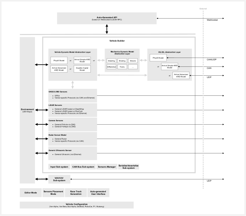
Figure 3: Overview of the racing simulator.

A.1 Client and Server Information Exchange

The agents and the racing simulator act together as a client-server system. The racing simulator includes both a physics and graphics engine and provides numerous communications mechanisms for a variety of use cases. Figure 3 summarises the simulator system architecture.

A.1.1 Simulator State

Management of the simulator’s state is done through a web-socket interface, allowing for two-way communication and for clients to update the state of the simulator including the ability to:

• Change the map

• Change the type of vehicle

• Change the pose of the vehicle

• Change the input mode

• Turn on/off debugging routines

• Turn on/off sensors

• Modify sensor parameters

• Modify vehicle parameters

A.1.2 Simulator-to-Agent Communication

The simulator communicates to agents primarily with sensory information including:

• LiDAR data from 4 independent sensors

• RADAR data from the vehicle’s radar sensor

• Images from the front-facing camera

• Pose information from the inertial measurement unit on the vehicle

• Additional data about the state of the vehicle such as brake pressure and tire speed per wheel

• Ground-truth information about other vehicles

• Ground-truth information about virtual objects

The camera publishes images using Transmission Control Protocol (TCP) while the others publish sensory data using User Data Protocol (UDP) or over a Controller Area Network (CAN). While the Learn-to-Race framework exclusively supports software-in-the-loop simulation, and therefore, only virtual CAN buses, the racing simulator also supports hardware-in-the-loop simulation and physical CAN buses.

A.1.3 Agent-to-Simulator Communication

Agents can communicate racing actions to the simulator in a variety of ways:

• Via a keyboard or joystick for human drivers

• UDP packets with steering, acceleration, and gear requests

• Through a safety layer with longitudinal acceleration and curvature requests

• Via various API modes which allow for more granular control of the vehicle including individual motor torques and brake pressure requests

Consistent with the simulator-to-agent above, agent-to-simulator communication can be done over virtual or physical CAN buses.

A.2 Additional Visualisation

The racing simulator features multiple real world racetracks each with unique features that challenge human and autonomous agents alike (see Figure 4).

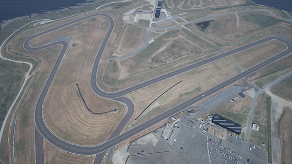
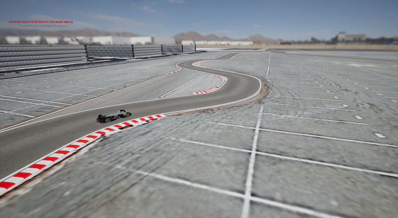
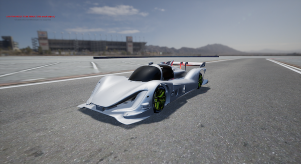
Figure 4: First column, top four rows: the Thruxton Circuit race track, United Kingdom, is infamous for its long straightaways, high speeds, and a difficult speed-trap near the finish line. Second column, top four rows: the North Road race track at Las Vegas Motor Speedway, United States, includes the sharp turns and merciless speed traps and adds a vision-processing challenge for learning agents, due to the lower contrast between the track and its surroundings. Third column, top four rows: the Anglesey Circuit race track, United Kingdom, features two prominent straights and several harrowing turns. Last row: the racing simulator features multiple car models, sensor placements, weather conditions, and additional tracks.

Appendix B Dataset Details

We generate a rich, multimodal dataset of expert demonstrations from the training racetracks (Track01:Thruxton and Track02:Anglesey), in order to facilitate pre-training of agents via, e.g., imitation learning (IL). The L2R dataset contains multi-sensory input at a 100-millisecond resolution, in both the observation and action spaces. See Table 1 in the main paper for a complete list of available modalities. The expert demonstrations were collected using a model predictive controller (MPC) that tracks the centerline of the race track at a pre-specified reference speed. Important parameters for this centerline MPC expert included acceleration range of [-1, 1], steering range of [-1, 1], and image H$\times$W dimensions of $384\times 512$. This training dataset contains 10,600 samples of each sensory and action dimension, in this first version, which includes 9 complete laps around the track. Demonstrations were saved as invidual step-wise transitions, using numpy.savez_compressed, with the following as dict fields in the data: (i) img with shape $(384,512,3)$; (ii) multimodal_data with shape $(30,)$; (iii) and action with shape $(2,)$. The fields in multimodal_data correspond to the vector dimension mappings, indicated in Table 5.

Table 5: Vector dimension mappings, to which the data fields in multimodal_data $(30,)$ correspond.

Array indices	Description
0	steering request
1	gear request
2	mode
3, 4, 5	directional velocity in $m/s$
6, 7, 8	directional acceleration in $m/s^{2}$
9, 10, 11	directional angular velocity
12, 13, 14	vehicle yaw, pitch, and roll, respectively
15, 16, 17	center of vehicle coordinates in $(y,x,z)$
18, 19, 20, 21	wheel revolutions per minute (per wheel)
22, 23, 24, 25	wheel braking (per wheel)
26, 27, 28, 29	wheel torque (per wheel)

Future version releases of L2R will include access to new simulated tracks (also modelled after real tracks, from around the world) as well as expert traces generated from these additional tracks—across various weather scenarios, in challenging multi-agent settings, and within dangerous obstacle-avoidance conditions.

Appendix C Additional Agent Details

C.1 RL-SAC Model Details

Table 6: RL-SAC model hyperparameters

Hyperparameter	Value
Buffer size	100,000
Gamma	0.99
Polyak	0.995
Learning rate	0.001
Alpha	0.2
Batch size	256
Start steps	1000
Learning steps	5

The RL-SAC agent learns from image embeddings rather than raw pixels. The encoder used is a convolutional variational autoencoder (VAE) which was trained prior to, and frozen during, the RL-SAC agent learning. The VAE was trained to encode RGB images of with a width and height of 144 pixels each into a latent space of size 32. The encoder architecture consisted of 4 convolutional layers, each followed by a ReLu activation, with a kernel size and stride of 4 and 2, respectively. The result of the convolutions was passed through a single fully connected layer to the compressed representation. Binary cross entropy loss and an Adam optimiser were used for training.

The RL-SAC agent was trained for 1,000 episodes which was approximately 1 million steps in the environment. We trained this agent in vision-only mode, so it only had access to the camera’s images. The agent passed the encoded images through two fully connected layers with 64 units each and a final layer with an output shape of 2, matching the environment’s action space. Gradient updates were taken at the conclusion of episodes, and the training hyperparameters are listed in Table 6.

C.2 MPC Agent Details

The MPC problem is summarised by Equation 5. The objective (Equation 5a) is to minimise the tracking error with respect to a reference trajectory, in this case the centerline of the race track at a pre-specified reference speed, with regularisation on actuations, over a planning horizon of T time steps. $\mathbf{Q}$ and $\mathbf{R}$ are both diagonal matrices corresponding to cost weights for tracking reference states and regularising actions. At the same time, the MPC respects the system dynamics of the vehicle (Equation 5b), and allowable action range (Equation 5c).

$$\min_{\mathbf{a}_{1:T}}\quad \sum_{t=1}^{T}\left[(\mathbf{s}_{t}-\mathbf{s}_{ref,i})^{T}\mathbf{Q}(\mathbf{s}_{i}-\mathbf{s}_{ref,i})+\mathbf{a}_{i}^{T}\mathbf{R}\mathbf{a}_{i}\right]$$ (5a)

s.t. $$\mathbf{s}_{t+1}=f(\mathbf{s}_{t},\mathbf{a}_{t}),\quad\forall t=1,\dots,T$$ (5b)

$$\underline{\mathbf{a}}\leq\mathbf{a}_{t}\leq\bar{\mathbf{a}}$$ (5c)

Specifically, we characterise the vehicle with the kinematic bike model [25] given in Equation 6, where the state is $\mathbf{s}=[x,y,v,\phi]$, and the action is $\mathbf{a}=[a,\delta]$. $x,y$ are the vehicle location in local east, north, up (ENU) coordinates, $v$ is the vehicle speed, and $\phi$ is the yaw angle (measured anti-clockwise from the local east-axis). $a$ is the acceleration, and $\delta$ is the steering angle at the front axle.

$$\dot{x} =v\cos(\phi)$$ (6a)

$$\dot{y} =v\sin(\phi)$$ (6b)

$$\dot{v} =a$$ (6c)

$$\dot{\phi} =v\tan{\delta}/L$$ (6d)

A key challenge is that the ground truth vehicle parameters were not known to us. Aside from $L$ defined as the distance between the front and rear axle, the kinematic bike model expects actions, i.e. acceleration and steering, in physical units, while the environment expects commands in $[-1,1]$. The mapping is unknown to us, and non-linear based on our observations. For instance, acceleration command = 1 results in smaller acceleration at higher speed. In the current implementation, we make a simplifying assumption that $a=k_{1}\times$ acceleration command, and $\delta=k_{2}\times$ steering command.

We use the iterative linear quadratic regulator (iLQR) proposed in [26], which iteratively linearizes the non-linear dynamics (Equation 6) along the current estimate of trajectory, solves a linear quadratic regulator problem based on the linearized dynamics, and repeats the process until convergence. Specifically, we used the implementation for iLQR from [4]. The parameters used by the MPC are summarised in Table 7.

Table 7: MPC parameters

Parameter	Value
$\mathbf{Q}$	$\text{diag}([1,1,1,16])$
$\mathbf{R}$	$\text{diag}([0.1,1])$
$v_{ref}$	12.5 m/s
$\mathbf{\bar{a}}$	$[1,0.2]$
$\mathbf{\underline{a}}$	$[-1,-0.2]$
$L$	2.7 m
$k_{1}$	10
$k_{2}$	6
$T$	6

Appendix D Metric Equations

We quantify the parametric curvature of a trajectory in Eqn. 7, with $x_{t}^{\prime}$ denoting $\frac{dx}{dt}$ at time $t$, and we summarise the curvature of the entire path as $\kappa_{rms}$ in Eqn. 8:

$$\kappa_{t}=\frac{x_{t}^{\prime}y_{t}^{\prime\prime}-y_{t}^{\prime}x_{t}^{\prime\prime}}{\Big{(}(x_{t}^{\prime})^{2}+(y_{t}^{\prime})^{2}\Big{)}^{\frac{3}{2}}}$$ (7)

$$\kappa_{rms}=\sqrt{\frac{1}{T}\left(\sum_{t=0}^{T}\kappa_{t}^{2}\right)}$$ (8)

We measure Trajectory efficiency as $\rho$ in Eqn. 9 based on the curvature, $\kappa_{rms}$, of the race track and the racing agent’s trajectory.

$$\rho=\frac{\kappa_{rms,\>racetrack}}{\kappa_{rms,\>trajectory}}$$ (9)

References

- [1] Indy autonomous challenge. https://www.indyautonomouschallenge.com/. Last accessed: 2021-01-30.
- [2] Roborace. https://roborace.com/. Last accessed: 2021-01-30.
- [3] Torcs, the open racing car simulator. http://torcs.sourceforge.net/index.php?name=Sections&op=viewarticle&artid=19. Last accessed: 2021-01-30.
- [4] Brandon Amos, Ivan Dario Jimenez Rodriguez, Jacob Sacks, Byron Boots, and J Zico Kolter. Differentiable mpc for end-to-end planning and control. arXiv preprint arXiv:1810.13400, 2018.
- [5] B. Balaji, S. Mallya, S. Genc, S. Gupta, L. Dirac, V. Khare, G. Roy, T. Sun, Y. Tao, B. Townsend, E. Calleja, S. Muralidhara, and D. Karuppasamy. Deepracer: Autonomous racing platform for experimentation with sim2real reinforcement learning. In 2020 IEEE International Conference on Robotics and Automation (ICRA), pages 2746–2754, 2020.
- [6] S. Balasubramanian, A. Melendez-Calderon, and E. Burdet. A robust and sensitive metric for quantifying movement smoothness. IEEE Transactions on Biomedical Engineering, 59(8):2126–2136, 2012.
- [7] J. Betz, A. Wischnewski, A. Heilmeier, F. Nobis, T. Stahl, L. Hermansdorfer, and M. Lienkamp. A software architecture for an autonomous racecar. In 2019 IEEE 89th Vehicular Technology Conference (VTC2019-Spring), pages 1–6, 2019.
- [8] G. Brockman, V. Cheung, L. Pettersson, J. Schneider, J. Schulman, J. Tang, and W. Zaremba. Openai gym, 2016.
- [9] Dian Chen, Brady Zhou, Vladlen Koltun, and Philipp Krähenbühl. Learning by cheating. In Conference on Robot Learning, pages 66–75. PMLR, 2020.
- [10] M. Chevalier-Boisvert, F. Golemo, Y. Cao, B. Mehta, and L. Paull. Duckietown environments for openai gym. https://github.com/duckietown/gym-duckietown, 2018.
- [11] Felipe Codevilla, Matthias M”uller, Antonio L’opez, Vladlen Koltun, and Alexey Dosovitskiy. End-to-end driving via conditional imitation learning. In 2018 IEEE International Conference on Robotics and Automation (ICRA), pages 4693–4700. IEEE, 2018.
- [12] P. Dhariwal, C. Hesse, O. Klimov, A. Nichol, M. Plappert, A. Radford, J. Schulman, S. Sidor, Y. Wu, and P. Zhokhov. Openai baselines. https://github.com/openai/baselines, 2017.
- [13] Wenhao Ding, Baiming Chen, Bo Li, Kim Ji Eun, and Ding Zhao. Multimodal safety-critical scenarios generation for decision-making algorithms evaluation. IEEE Robotics and Automation Letters, 6(2):1551–1558, 2021.
- [14] Alexey Dosovitskiy, German Ros, Felipe Codevilla, Antonio Lopez, and Vladlen Koltun. CARLA: An open urban driving simulator. In Proceedings of the 1st Annual Conference on Robot Learning, pages 1–16, 2017.
- [15] Benjamin Eysenbach and Sergey Levine. Maximum entropy rl (provably) solves some robust rl problems. arXiv preprint arXiv:2103.06257, 2021.
- [16] Angelos Filos, Panagiotis Tigas, Rowan McAllister, Nicholas Rhinehart, Sergey Levine, and Yarin Gal. Can autonomous vehicles identify, recover from, and adapt to distribution shifts? In International Conference on Machine Learning (ICML), 2020.
- [17] F. Florian, S. Yunlong, E. Kaufmann, D. Scaramuzza, and P. Duerr. Super-human performance in gran turismo sport using deep reinforcement learning, 2020.
- [18] Jonathan Francis, Nariaki Kitamura, Felix Labelle, Xiaopeng Lu, Ingrid Navarro, and Jean Oh. Core challenges in embodied vision-language planning. arXiv preprint arXiv:2106.13948, 2021.
- [19] David Fridovich-Keil, Andrea Bajcsy, Jaime F Fisac, Sylvia L Herbert, Steven Wang, Anca D Dragan, and Claire J Tomlin. Confidence-aware motion prediction for real-time collision avoidance1. The International Journal of Robotics Research, 39(2-3):250–265, 2020.
- [20] Javier Garcıa and Fernando Fernández. A comprehensive survey on safe reinforcement learning. Journal of Machine Learning Research, 16(1):1437–1480, 2015.
- [21] T. Haarnoja, A. Zhou, P. Abbeel, and S. Levine. Soft actor-critic: Off-policy maximum entropy deep reinforcement learning with a stochastic actor. In Jennifer Dy and Andreas Krause, editors, Proceedings of the 35th International Conference on Machine Learning, volume 80 of Proceedings of Machine Learning Research, pages 1861–1870, Stockholmsmässan, Stockholm Sweden, 10–15 Jul 2018. PMLR.
- [22] T. Herrmann, F. Passigato, J. Betz, and M. Lienkamp. Minimum race-time planning-strategy for an autonomous electric racecar. 2020 IEEE 23rd International Conference on Intelligent Transportation Systems (ITSC), Sep 2020.
- [23] T. Herrmann, A. Wischnewski, L. Hermansdorfer, J. Betz, and M. Lienkamp. Real-time adaptive velocity optimization for autonomous electric cars at the limits of handling. IEEE Transactions on Intelligent Vehicles, pages 1–1, 2020.
- [24] D. P. Kingma and M. Welling. Auto-Encoding Variational Bayes. In 2nd International Conference on Learning Representations, ICLR 2014, Banff, AB, Canada, April 14-16, 2014, Conference Track Proceedings, 2014.
- [25] Jason Kong, Mark Pfeiffer, Georg Schildbach, and Francesco Borrelli. Kinematic and dynamic vehicle models for autonomous driving control design. In 2015 IEEE Intelligent Vehicles Symposium (IV), pages 1094–1099. IEEE, 2015.
- [26] Weiwei Li and Emanuel Todorov. Iterative linear quadratic regulator design for nonlinear biological movement systems. In ICINCO (1), pages 222–229. Citeseer, 2004.
- [27] D. Loiacono, L. Cardamone, and P. L. Lanzi. Simulated car racing championship: Competition software manual. arXiv preprint arXiv:1304.1672, 2013.
- [28] Seong Hyeon Park, Gyubok Lee, Manoj Bhat, Jimin Seo, Minseok Kang, Jonathan Francis, Ashwin R Jadhav, Paul Pu Liang, and Louis-Philippe Morency. Diverse and admissible trajectory forecasting through multimodal context understanding. In European Conference on Computer Vision (ECCV), 2020.
- [29] L. Paull, J. Tani, H. Ahn, J. Alonso-Mora, L. Carlone, M. Cap, Y. F. Chen, C. Choi, J. Dusek, Y. Fang, D. Hoehener, S. Liu, M. Novitzky, I. F. Okuyama, J. Pazis, G. Rosman, V. Varricchio, H. Wang, D. Yershov, H. Zhao, M. Benjamin, C. Carr, M. Zuber, S. Karaman, E. Frazzoli, D. Del Vecchio, D. Rus, J. How, J. Leonard, and A. Censi. Duckietown: An open, inexpensive and flexible platform for autonomy education and research. In 2017 IEEE International Conference on Robotics and Automation (ICRA), pages 1497–1504, 2017.
- [30] K. Shao, Z. Tang, Y. Zhu, N. Li, and D. Zhao. A survey of deep reinforcement learning in video games, 2019.
- [31] T. Stahl, A. Wischnewski, J. Betz, and M. Lienkamp. Multilayer graph-based trajectory planning for race vehicles in dynamic scenarios. In 2019 IEEE Intelligent Transportation Systems Conference (ITSC), pages 3149–3154, 2019.
- [32] Y. Tassa, Y. Doron, A. Muldal, T. Erez, Y. Li, D. de Las Casas, D. Budden, A. Abdolmaleki, J. Merel, A. Lefrancq, T. Lillicrap, and M. Riedmiller. Deepmind control suite, 2018.
- [33] E. Todorov, T. Erez, and Y. Tassa. Mujoco: A physics engine for model-based control. In 2012 IEEE/RSJ International Conference on Intelligent Robots and Systems, pages 5026–5033, 2012.