Switching Controller Synthesis for Delay Hybrid Systems
under Perturbations

Abstract.

Delays are ubiquitous in modern hybrid systems, which exhibit both continuous and discrete dynamical behaviors. Induced by signal transmission, conversion, the nature of plants, and so on, delays may appear either in the continuous evolution of a hybrid system such that the evolution depends not only on the present state but also on its execution history, or in the discrete switching between its different control modes. In this paper we come up with a new model of hybrid systems, called delay hybrid automata, to capture the dynamics of systems with the aforementioned two kinds of delays. Furthermore, based upon this model we study the robust switching controller synthesis problem such that the controlled delay system is able to satisfy the specified safety properties regardless of perturbations. To the end, a novel method is proposed to synthesize switching controllers based on the computation of differential invariants for continuous evolution and backward reachable sets of discrete jumps with delays. Finally, we implement a prototypical tool of our approach and demonstrate it on some case studies.

1. Introduction

With the broad applications of cyber-physical systems (CPS) in our daily life, the correct design of reliable CPS is getting increasingly important, especially in safety-critical domains such as automotive, medicine, etc. Due to the bidirectional conversion between analog and digital signals, the periodicity of collecting data by sensors, and executing the commands by actuators, and the data transmission through networks with different bandwidths, etc., time delay is becoming ubiquitous and inevitable in CPS, giving rise to the difficulty of CPS design, as delays may invalidate the certificates of stability and safety obtained with abstracting them away, even well annihilate control performance.

Generally, two kinds of delays appear commonly in CPS. One is in continuous evolution of systems, resulting in that the evolution not only depends on the current state, but also on the historical states. As an appropriate generalization of ordinary differential equations (ODEs), delay differential equations (DDEs) are widely used to capture time-delay continuous dynamical systems. The other one occurs at discrete jumps between different control modes of the underlying systems.

In this paper, we propose a new model of hybrid systems, called delay hybrid automata (dHA), which is an extension of classical hybrid automata (HA) (Henzinger et al., 1995), in order to capture the dynamics of systems involving the aforementioned two kinds of delays. Based on the proposed dHA, we investigate the safe switching controller synthesis problem for delay hybrid systems, i.e., given a dHA $\mathcal{H}$ and a safety property $\mathcal{S}$, to synthesize a refined dHA $\mathcal{H}^{*}$ by strengthening the invariant in each mode and the guard condition for each discrete jump such that $\mathcal{H}^{*}$ satisfies $\mathcal{S}$ robustly, with additional condition that $\mathcal{H}^{*}$ is non-blocking if $\mathcal{H}$ is non-blocking. Our approach is invariant-based, which is a classical approach to synthesizing safe switching controllers for HA (Asarin et al., 2000; Zhao et al., 2013). However, the computation of differential invariants (the definition will be given in Section 3) for the DDE in each mode as well as a global invariant (the definition will be given in Section 4.2) among these modes is much involved than the counterparts in HA when the two kinds of delays are considered. To compute differential invariants for DDEs, we propose a two-step approach: the first step is to reduce differential invariant generation problem to $T$-differential invariant generation problem using global ball-convergence condition derived in terms of Metzler matrix for a class of linear DDEs, where $T$ is a bounded time horizon; the second step is to obtain an over-approximation of the $T$-bounded reachable set based on the growth bound adapted from (Reissig et al., 2017). Non-linear DDEs can be reduced to the linear case by means of the linearization technique, in case that global ball-convergence is replaced by local ball-convergence. A global invariant is generated based on fixed point iteration, and the computation of differential invariants for continuous evolution in each mode and backward reachable sets for discrete jumps by taking delays into account, which is similar to compute reachable sets of HA, e.g., with dReach (Kong et al., 2015). Our approach is finally illustrated on some interesting case studies.

The main contributions of this work are summarized below:

• a new model language, called dHA, is proposed to model delay hybrid systems, which exhibit delays in both continuous- and discrete-time dynamics.

• in this new model dHA, a novel approach based on the computation of differential invariants is proposed to address the switching controller synthesis problem for delay hybrid systems, such that the controlled delay hybrid system is able to satisfy the specified safety property.

1.1. Related Work

Controller synthesis through correct-by-construction manner provides mathematical guarantees to the correctness and reliablity of (hybrid) systems. In the literature, this problem has been extensively studied and various approaches have been proposed, which can be categorized into abstraction based, e.g., (P.Tabuada, 2009; Belta et al., 2017; Girard, 2012; Reissig et al., 2017; Nilsson et al., 2017; Hsu et al., 2018), and constraint solving based, e.g., (Zhao et al., 2013; Taly and Tiwari, 2010). The basic idea of abstraction based approaches is to abstract the original system under consideration to a finite-state two-players game, and then solve reactive synthesis using automata-theoretic algorithms with respect to temporal control objectives. In contrast, the basic idea of constrains solving based approaches is to reduce the synthesis problem to an invariant generation problem, which can be further reduced to a constraint solving problem. As a generalization of (Taly and Tiwari, 2010), an optimal switching controller synthesis is investigated in (Jha et al., 2011) by solving an unconstrained numerical optimization problem. Based on reachable set computation and fixed point iteration, a general framework of controller synthesis for HA is proposed in (Asarin et al., 2000; Tomlin et al., 2000). However, all these existing works focus on ODEs, therefore cannot be applied to DDEs, let alone delay hybrid systems directly. This is because ODEs are Markovian, but DDEs are non-Markovian, whose states are functionals with infinite dimension. In (Chen et al., 2018; Chen et al., 2020), a controller synthesis problem for time-delay discrete dynamical systems was first investigated by reduction to solving imperfect two-player safety game, but it is unclear whether their approach can be extended to time-delay continuous dynamical systems and delay hybrid systems.

Recently, verification and synthesis for time-delay systems attract increasing attention, we just name a few below. Prajna and Jadbabaie extended the notion of barrier certificate to time-delay systems (Prajna and Jadbabaie, 2005). In (Zou et al., 2015), Zou et al. first proposed interval Taylor model for DDEs, and then discussed automatic stability analysis and safety verification based on interval Taylor model and stability analysis of discrete dynamical systems. However, their approach can only be applied to specific DDEs, whose right sides are independent of current states. Following this line, more efficient algorithms for analyzing Taylor models to inner and outer approximate reachable sets of more general DDEs in finite time horizon were given (Goubault and Putot, 2019). In (Feng et al., 2019), Feng et al. further considered how to utilize stability analysis of linear delay dynamical systems and linearization to reduce the unbounded verification to the bounded verification for a class of general DDEs. Based on (Feng et al., 2019), (Bai et al., 2021) investigated switching controller synthesis problem of delay hybrid systems, in which time-delay in discrete jumps is not taken into account. In contrast, the approach proposed in this paper can compute differential invariants for DDEs using ball-convergence based on Metzler matrix analysis, growth bound and linearization, it could be more powerful and applied to verify more DDEs (see Example 4). In (Chen et al., 2016), a simulation-based approach to approximate reachable sets of ODEs was extended to DDEs. Meanwhile, a topological homeomorphism-based approach was proposed to over- and under-approximate reachable sets of a class of DDEs (Xue et al., 2017). Later, this approach was further extended to deal with perturbed DDEs in (Xue et al., 2021). Like (Goubault and Putot, 2019), these approaches can only be applied to compute reachable sets in finite time horizon. In addition, in (Pola et al., 2010, 2015), Pola et al. proposed approaches how to construct symbolic abstractions for time-invariant and time-varying delay systems by approximating functional space using spline analysis. In (Huang et al., 2017), Huang et al. proposed a bounded verification method for nonlinear networks with discrete delays. Nonetheless, the dynamics of each subsystem modelled by ODEs and the analysis is done over a finite time horizon. Evidently, only one kind of delays is considered in all these existing works, either continuous or discrete. There is indeed a lack of appropriate formal models to handle both situations uniformly.

1.2. A Motivating Example

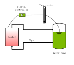
Figure 1. A heating system

To illustrate the main idea of our approach, we use a heating system as a motivating example, as depicted in Fig. 1, consisting of the following four components:

• a water tank with water,

• a heater with on and off two states,

• a thermometer monitoring the temperature of the water in the tank, and echoing warning signals whenever the temperature of the water is above or below certain thresholds,

• pipes connecting the heater and the tank.

Additionally, we add a controller that observes the signals produced in the thermometer, and computes a command to the heater in order to maintain the temperature of the water within a given range. The temperature of water in the tank is desired to stay between $20$ and $90$ degrees through switching the heating on and off. The behavior of the temperature of water in the tank is mixed continuous evolution with discrete switches, which can be modelled by a hybrid automaton (Alur et al., 1995). However, the delay impact of pipes and thermometer monitoring are both neglected in these models. In (Richard Kicsinya, 2012), it was pointed out that energy efficiency can be increased by $5-10\%$ if the delay impact of pipes is considered. Moreover, due to the delay possibly caused by measuring the thermometer, sending the signals, executing the control commands and so on, the temperature of water in the tank could be beyond the thresholds, which is definitely unsafe. Therefore, the delay impacts of the pipes and the thermometer have to be taken into account when we model the temperature of water in the tank.

1.3. Basic Notations and Definitions

Notations. Let $\mathbb{N}$, $\mathbb{R}$ and $\mathbb{C}$ be the set of natural, real and complex numbers, $\mathbb{R}_{+}$ be the set of positive real numbers. For $z=a+ib\in\mathbb{C}$ with $a,b\in\mathbb{R}$, $\Re(z)=a$ and $\Im(z)=b$, respectively, denote the real and imaginary parts of $z$. $\mathbb{R}^{n}$ is the set of $n$-dimensional real vectors, denoted by boldface letters. Given a vector $\mathbf{x}\in\mathbb{R}^{n}$, $x_{i}$ denotes the $i$-th coordinate of $\mathbf{x}$ for $i\in\{1,2,\ldots,n\}$, and its maximal norm is $\|\mathbf{x}\|_{\infty}=\max_{1\leq i\leq n}|x_{i}|$. For a vector $\mathbf{y}\in\mathbb{R}^{n}_{+}$, let $(\mathbf{y})_{\min}=\min_{1\leq i\leq n}y_{i}$. Given two vectors $\mathbf{x},\mathbf{y}\in\mathbb{R}^{n}$, we define $\mathbf{x}\geq\mathbf{y}$ iff $x_{i}\geq y_{i}$ for all $1\leq i\leq n$, and $\mathbf{x}>\mathbf{y}$ iff $x_{i}>y_{i}$ for all $1\leq i\leq n$. Given $\epsilon>0$, we define $\mathfrak{B}(\epsilon)=\{\mathbf{x}\in\mathbb{R}^{n}\mid\|\mathbf{x}\|_{\infty}\leq\epsilon\}$ as the $\epsilon$-closed ball around $\mathbf{0}$. Let $\mathbb{R}^{n\times m}$ be the set of real $n\times m$ matrices. The entry in the $i$-th row and $j$-th column of a matrix $M\in\mathbb{R}^{n\times m}$ is denoted as $m_{ij}$ with $1\leq i\leq n$ and $1\leq j\leq m$. For $t_{1}<t_{2}$, $\mathcal{C}\{[t_{1},t_{2}],\mathbb{R}^{n}\}$ is the space of continuous functions from $[t_{1},t_{2}]$ to $\mathbb{R}^{n}$. For a set $\mathbb{A}\subseteq\mathbb{R}_{+}^{n}$, $\mathbf{a}=\sup\mathbb{A}$ iff for all $\mathbf{x}\in\mathbb{A}$, $\mathbf{x}\leq\mathbf{a}$, and for any upper bound $\mathbf{y}\in\mathbb{R}_{+}^{n}$, then $\mathbf{y}\geq\mathbf{a}$. Finally, we denote $(x)^{+}=\max(0,x)$ for any real number $x\in\mathbb{R}$.

In this paper, we consider a class of time-delay systems under perturbations described as follows:

(1) $$\left\{\begin{array}[]{lr}\dot{\mathbf{x}}(t)=\bm{f}(\mathbf{x}(t),\mathbf{x}(t-r_{1}),\ldots,\mathbf{x}(t-r_{k}),\mathbf{w}(t)),&t\in[0,\infty)\\ \mathbf{x}(t)=\bm{\phi}(t),&t\in[-r_{k},0]\end{array}\right.$$

where $\mathbf{x}\in\mathbb{R}^{n}$ is the state vector, $t\in\mathbb{R}$ models time, The discrete delays are assumed to satisfy $0<r_{1}<r_{2}<\cdots<r_{k}$. $\mathbf{w}(\cdot):[0,\infty)\mapsto\mathbb{R}^{m}$ is external disturbance vector, which is unknown but assumed to be bounded by a given constant $w_{max}$, i.e., $\|\mathbf{w}(t)\|_{\infty}\leq w_{max}$ for all $t\geq 0$. $\bm{\phi}(\cdot)\in\mathcal{C}\{[-r_{k},0],\mathbb{R}^{n}\}$ is the initial condition. Suppose that $\bm{f}$ is continuous and satisfies the Lipschitz condition, then from a given initial condition $\bm{\phi}$ and $\mathbf{w}(t)$, there exists a unique solution $\bm{\xi_{\phi}}^{\mathbf{w}}(\cdot):[-r_{k},\infty)\mapsto\mathbb{R}^{n}$.

Definition 0 (Metzler matrix(Berman and Plemmons, 1994)).

A matrix $M\in\mathbb{R}^{n\times n}$ is called a Metzler matrix if all off-diagonal elements of $M$ are non-negative, i.e., $m_{ij}\geq 0$ whenever $i\neq j$.

Regarding Metzler matrices, the following proposition holds, please refer to (Berman and Plemmons, 1994) for the detail.

Proposition 0 ((Berman and Plemmons, 1994)).

For any Metzler matrix $M$, the following two properties are equivalent

• $\mu(M)<0$, where $\mu(M)=\max\{\Re(\alpha)\mid\alpha\in\mathbb{C}:\det(\alpha\mathcal{I}-M)=0)\}$, $\mathcal{I}$ is the $n\times n$ identity matrix.

• there exists $\bm{\zeta}\in\mathbb{R}^{n}$ and $\bm{\zeta}>\bm{0}$ such that $M\bm{\zeta}<\bm{0}$.

The structure of this paper is organized as: the notion of delay hybrid automata and the safe switching controller synthesis problem of interest are defined in Section 2. After presenting an approach for invariant generation of delay hybrid systems in Section 3, Section 4 concentrates on the controller synthesis framework based on the global invariants generation for delay hybrid systems. We demonstrate our approach with two examples in Section 5. Finally Section 6 concludes this paper.

2. Delay Hybrid Automata and Problem Statement

Hybrid automata (HA) (Henzinger et al., 1995) are popular models for dynamical systems with complex mixed continuous-discrete behaviors. In order to characterize behaviors of hybrid systems with the two type of time delays aforementioned, we introduce an extension of HA, called delay hybrid automata (dHA), formally defined as follows:

Definition 0 (Delay hybrid automaton, dHA).

A dHA is a tuple $\mathcal{H}=(Q,X,U,I,\Xi,F,E,D,G,R)$, where,

• $Q=\{q_{1},\ldots,q_{m}\}$ is a finite set of modes;

• $X$ is a set of state variables;

• $U\subseteq\mathcal{C}\{[t_{1},t_{2}],\mathbb{R}^{n}\}$, where $t_{1}<t_{2}$, is a set of continuous functionals;

• $I:Q\mapsto 2^{\mathbb{R}^{n}}$ gives each mode $q\in Q$ an invariant $I(q)\subseteq\mathbb{R}^{n}$;

• $\Xi:Q\mapsto 2^{U}$ gives each mode $q\in Q$ its initial states set $\Xi(q)\subseteq U$;

• $F=\{\bm{f}_{q_{1}},\ldots,\bm{f}_{q_{m}}\}$ is the set of vector fields, each mode $q\in Q$ has unique vector field $\bm{f}_{q}$, which is used to form a delayed differential equation (1) to model the continuous evolution, i.e.,

  $$\dot{\mathbf{x}}(t)=\bm{f}_{q}(\mathbf{x}(t),\mathbf{x}(t-r^{q}_{1}),\ldots,\mathbf{x}(t-r^{q}_{k}),\mathbf{w}(t));$$

• $E\subseteq Q\times Q$ is the set of discrete transition relations between modes;

• $D:E\mapsto\mathbb{R}_{+}$ gives each discrete transition $e\in E$ a delay time $D(e)\in\mathbb{R}_{+}$;

• $G:E\mapsto 2^{\mathbb{R}^{n}}$ denotes guard conditions;

• $R:E\times X_{D}\mapsto U$ denotes reset functions.

Compared with the definition of HA, there are several notable changes in Definition 1: a new item $U\subseteq\mathcal{C}\{[-r_{k}^{q},0],\mathbb{R}^{n}\}$ is introduced to represent the set of all possible initial states. Note that the solution to a DDE is a functional, and correspondingly a state is a function standing the execution history up to the considered instant starting from the given initial state, rather than a point in $\mathbb{R}^{n}$ as for ODE. Additionally, another new item $D$ is used to specify the delays in discrete transitions: for each $e=(q,q^{\prime})\in E$, the delay is denoted by $D(e)\in\mathbb{R}_{+}$. Moreover, the reset function $R$ is changed to $E\times X_{D}\mapsto U$ accordingly, where $X_{D}$ is the set of reachable states satisfying the corresponding guard condition. Intuitively, when a mode switching happens, e.g., a transition from $q$ to $q^{\prime}$ at time $t$, there exists time $\theta\in[-r_{k}^{q},0]$, the system has to satisfy: $\mathbf{x}_{t}^{\bm{\phi}}(\theta)\in G(e)$, and the update state is $\bm{\phi}^{\prime}=R(e,\mathbf{x}_{t+D(e)}^{\bm{\phi}}(\cdot))$.

Example 0.

For the heating system shown in the motivating example, it is straightforward to present its dHA textually as follows:

• $Q=\{q_{1},q_{2}\}$; (two modes of discrete states, heater on and off);

• $X=\{x\}$; (the temperature of water in the tank);

• $U=\mathcal{C}$; (all continuous functionals);

• $I(q_{1})=\{x\in\mathbb{R}\mid 20\leq x\leq 90\}$ and $I(q_{2})=\{x\in\mathbb{R}\mid 20\leq x\leq 90\}$;

• $\Xi(q_{1})=\{x(t)\mid x(t)=50-10\sin{t},t\in[-1,0]\}$ and $\Xi(q_{2})=\{x(t)\mid x(t)=85-5\sin{t},t\in[-1,0]\}$;

• $F=\{f_{q_{1}},f_{q_{2}}\}$, where $f_{q_{1}}=K_{1}(h-x(t))+K_{2}x(t-1)+w_{1}$ and $f_{q_{2}}=-K_{1}x(t)+K_{2}x(t-1)+w_{2}$, $K_{1}$, $K_{2}$, $h$, $w_{1}$ and $w_{2}$ are real constants. That is, the temperature rises and decreases following the respective DDE in $q_{1}$ and $q_{2}$, respectively;

• $E=\{e_{1}=(q_{1},q_{2}),e_{2}=(q_{2},q_{1})\}$;

• $D(e_{1})=2$ and $D(e_{2})=2$;

• $G(e_{1})=\mathbb{R}$ and $G(e_{2})=\mathbb{R}$;

• $R(e_{1},x_{t+D(e_{1})}(\cdot))=x(\theta),\theta\in[t+D(e_{1})-1,t+D(e_{1})]$ with $x(t)\in G(e_{1})$ and $R(e_{2},x_{t+D(e_{1})}(\cdot))=x(\theta),\theta\in[t+D(e_{2})-1,t+D(e_{2})]$ with $x(t)\in G(e_{2})$.

Pictorially, the dHA is shown in Fig. 2.

Figure 2. The dHA for the heating system

Definition 0 (Hybrid execution).

For a dHA $\mathcal{H}$, given an initial hybrid state $(q_{0},\bm{\xi}^{\mathbf{w}}_{\bm{\phi}_{0}}(0))$ and $\mathbf{w}(\cdot):[0,\infty)\mapsto\mathbb{R}^{m}$, an execution $\pi$ of the delay hybrid automaton $\mathcal{H}$ is a sequence of $\langle t_{i},q_{i},\bm{\xi}_{\bm{\phi}_{i}}^{\mathbf{w}}(t_{i})\rangle$, for $i\in\mathbb{N}$ and $q_{i}\in Q$, satisfying that any transition $\langle t_{i},q_{i},\bm{\xi}^{\mathbf{w}}_{\bm{\phi}_{i}}(t_{i})\rangle\mapsto\langle t_{i+1},q_{i+1},\bm{\xi}_{\bm{\phi}_{i+1}}^{\mathbf{w}}(t_{i+1})\rangle$ is either :

• the continuous evolution: $q_{i}=q_{i+1}$, $\bm{\phi}_{i}=\bm{\phi}_{i+1}$, $t_{i}<t_{i+1}$, and for all $t\in[t_{i},t_{i+1}]$, the solution of DDE $\dot{\mathbf{x}}=\bm{f}_{q_{i}}$ is $\bm{\xi}_{\bm{\phi}_{i}}^{\mathbf{w}}(\cdot):[t_{i},t_{i+1}]\mapsto\mathbb{R}^{n}$, and $\bm{\xi}_{\bm{\phi}_{i}}^{\mathbf{w}}(t)\in I(q_{i})$;

• the discrete transition: $e=(q_{i},q_{i+1})\in E$, $t_{i}=t_{i+1}$, and there exists $t$ such that $t_{i+1}=t+D(e)$ and $\bm{\xi}_{\bm{\phi}_{i}}^{\mathbf{w}}(t)\in G(e)$ and $\bm{\phi}_{i+1}=R(e,\mathbf{x}_{t+D(e)}^{\bm{\phi}_{i}}(\cdot))$.

An execution $\pi$ is called finite if it is a finite sequence ending with a closed time interval. Otherwise, the execution $\pi$ is called infinite if it is an infinite sequence or if $\sum_{i=0}^{N}(t_{i+1}-t_{i})=\infty$, where $N\in\mathbb{N}$. A dHA $\mathcal{H}$ is called non-blocking if there exists at least one infinite execution starting from any initial state.

Definition 0 (Reachable set).

Given a dHA $\mathcal{H}$, the reachable set $\mathrm{R}_{\mathcal{H}}(t)$ for the delay hybrid system within $[-r^{q_{0}}_{k},t]$ is

$$\mathrm{R}_{\mathcal{H}}(t)=\left\{\mathbf{x}(t)\,\middle|\,\begin{array}[]{cc}\forall\,q_{0}\in Q,\,\forall\,\bm{\xi}^{\mathbf{w}}_{\bm{\phi}_{0}}(0)\in\Xi(q_{0}),\\ \exists\,\pi=\langle t_{0},q_{0},\bm{\xi}^{\mathbf{w}}_{\bm{\phi}_{0}}(0)\rangle,\cdots,\langle t,q_{i},\bm{\xi}_{\bm{\phi}_{i}}^{\mathbf{w}}(t)\rangle\\ s.t.\,\mathbf{x}(t)=\bm{\xi}_{\bm{\phi}_{i}}^{\mathbf{w}}(t)\end{array}\right\}.$$

Example 0.

An execution for the heating system in the motivating example is given below.

From the initial state $(q_{1},x=50.00)$, the system reaches the state $(q_{1},x=68.86)$ in green after $10s$, which is indicated by transition $(1)$. Assume that the state $(q_{1},x=68.86)$ in green satisfies the guard condition, the system chooses to jump from mode $q_{1}$ to mode $q_{2}$. However, there is a delay $D(e_{1})=2$ incurred by the edge $e_{1}$. The system keeps evolving in mode $q_{1}$ until hitting the state $(q_{1},x=71.12)$ revealed by transition $(2)$, and completes the switching by reaching the state $(q_{2},x=71.12)$ displayed by transition $(3)$ in blue. Continue this execution as above.

Definition 0 (Safety).

Given a dHA $\mathcal{H}$ with a safe set $\mathcal{S}=\cup_{q\in Q}\mathcal{S}_{q}$, where $\mathcal{S}_{q}\subseteq\mathbb{R}^{n}$, the automaton $\mathcal{H}$ is $T$-safe with respect to $\mathcal{S}$ in time $T$, if for any time $t\in[-r^{q}_{k},T]$, all reachable states $\mathrm{R}_{\mathcal{H}}(t)$ of the system starting from any initial states are contained in $\mathcal{S}$, i.e.,

$$\mathrm{R}_{\mathcal{H}}(t)\subseteq\mathcal{S},\forall t\in[-r^{q}_{k},T].$$

If $T$ is infinite, then the dHA is safe over the infinite-time horizon.

Now, the problem of interest can be formally formulated as follows:

Problem 1 (Safe Switching Controller Synthesis Problem).

Given a dHA $\mathcal{H}=(Q,X,U,I,\Xi,F,E,D,G,R)$ and a safety property $\mathcal{S}$, the switching controller problem is to synthesize a new dHA $\mathcal{H}^{*}=(Q,X,U^{*},I^{*},\Xi^{*},F,E,D,G^{*},R)$ such that $\mathcal{H}^{*}$ satisfies:

1. $\mathcal{H}^{*}$ is safe, i.e. in $[-r^{q}_{k},\infty)$, the reachable set $\mathrm{R}_{\mathcal{H}^{*}}\subseteq\mathcal{S}$.

2. $\mathcal{H}^{*}$ is a refinement of $\mathcal{H}$, i.e., it holds: $\Xi^{*}\subseteq\Xi\cap\mathcal{S}$, $I^{*}\subseteq I$, $U^{*}\subseteq U$, and for any $e\in E$, it holds: $\forall\mathbf{x}(t)\in G^{*}(e)$, $\mathbf{x}(t+D(e))\in G(e)\cap I^{*}(q)$.

3. if $\mathcal{H}$ is non-blocking in the safe set $\mathcal{S}$, then $\mathcal{H}^{*}$ is non-blocking.

$SC=\{G^{*}(e)\subseteq\mathbb{R}^{n}\mid e\in E\}$ is called a safe switching controller of $\mathcal{H}$, if $\mathcal{H}^{*}$ satisfies above three requirements. We call $SC$ is a trivial switching controller of $\mathcal{H}$, if there exists one mode $q\in Q$ or one edge $e\in E$ with $I^{*}(q)=\emptyset$ or $G^{*}(e)=\emptyset$.

3. Differential Invariant Generation

Differential invariant generation plays a central role in our framework to synthesize switching controllers for delay hybrid systems with perturbations. In this section, inspired by the work in (Feng et al., 2019), we present a two-step procedure to synthesize differential invariants for a delay dynamical system. The first step is to calculate a bounded horizon $T$ using ball convergence analysis, which reduces the differential invariant generation problem to the $T$-differential invariant generation problem. The second step is to compute an over-approximation of the reachable set in time $T$, which is a $T$-differential invariant.

We first develop the aforementioned two-step method for linear delay dynamical systems, and then generalize it to nonlinear delay dynamical systems.

Definition 0 (Differential invariant).

Given a mode $q\in Q$ of a delay hybrid automaton $\mathcal{H}$: $(\Xi(q),\bm{f}_{q},I(q))$ and time $T$, a set $I^{*}(q)$ is called a $T$- invariant if for any trajectory starting from a given initial function $\bm{\phi}(t)\in\Xi(q)$, $t\in[-r^{q}_{k},0]$, the following condition holds for $\mathbf{w}(\cdot):[-r^{q}_{k},T]\mapsto\mathbb{R}^{m}$:

$$\forall t\in[-r^{q}_{k},T],\ \bm{\xi}_{\bm{\phi}}^{\mathbf{w}}(t)\in I(q)\implies\forall t\in[-r^{q}_{k},T],\bm{\xi}_{\bm{\phi}}^{\mathbf{w}}(t)\in I^{*}(q).$$

If $T$ is infinite, then $I^{*}(q)$ is a differential invariant of mode $q$.

$T$- invariant $I^{*}(q)$ requires that every trajectory starting from initial set $\Xi(q)$ in time $T$ remains inside the differential invariant $I^{*}(q)$ if it remains in the domain $I(q)$. A safe differential invariant requires $I^{*}(q)\subseteq\mathcal{S}_{q}$.

3.1. Linear Systems

We consider linear DDEs with the form (1) first, i.e.,

(2) $$\left\{\begin{array}[]{lr}\dot{\mathbf{x}}(t)=A\mathbf{x}(t)+B\mathbf{x}(t-r)+C\mathbf{w}(t),&t\in[0,\infty)\\ \mathbf{x}(t)=\bm{\phi}(t),&t\in[-r,0]\end{array}\right.\,,$$

where $A,B\in\mathbb{R}^{n\times n}$ and $C\in\mathbb{R}^{n\times m}$ are real matrices with appropriate dimensions.

Definition 0 (Global ball-convergence).

Given a $\mathfrak{r}>0$, (2) is called globally exponentially convergent within the ball $\mathfrak{B}(\mathfrak{r})$, if there exist a constant $\gamma>0$ and a non-decreasing function $\kappa(\cdot)$ such that

$$\|\bm{\xi}_{\bm{\phi}}^{\mathbf{w}}(t)\|_{\infty}\leq\mathfrak{r}+\kappa(\|\bm{\phi}\|_{\infty})\mathrm{e}^{-\gamma t},\ \forall t\geq 0$$

holds for all $\bm{\phi}\in\mathcal{C}\{[-r,0],\mathbb{R}^{n}\}$ and $\|\mathbf{w}(t)\|_{\infty}\leq w_{max},\forall t\geq 0$.

In Definition 2, $\gamma$ represents the rate of decay, i.e., an estimate of how quickly the solution of (2) converges to the ball $\mathfrak{B}(\mathfrak{r})$. Especially, when the radius $\mathfrak{r}=\mathbf{0}$, the definition of ball convergence is consistent with Lyapunov exponential stability (Lyapunov, 1992). Moreover, in (Hien and Trinh, 2014), it was proved that

Theorem 3 ((Hien and Trinh, 2014)).

Suppose in (2) $M=A+B$ is a Metzler matrix satisfying one of the properties in Proposition  2. Then, there exist positive constants $\beta$, $\gamma$, $\delta$, $\eta$ such that for all initial functions $\bm{\phi}$ and $\|\mathbf{w}(t)\|_{\infty}\leq w_{max},\forall t\geq 0$

$$\|\bm{\xi}_{\bm{\phi}}^{\mathbf{w}}(t)\|_{\infty}\leq\frac{C_{max}w_{max}}{\eta}+\beta(\|\bm{\phi}\|_{\infty}-\frac{C_{max}w_{max}}{\delta})^{+}\mathrm{e}^{-\gamma t},\ \forall t\geq 0$$

holds, where $C_{max}=\max_{i\in n}\sum_{j=1}^{m}C_{ij}$.

In Theorem 3, based on the notion of Metzler matrix, (2) is globally exponentially convergent to the ball $\mathfrak{B}(\frac{C_{max}w_{max}}{\eta})$ for all perturbations $\|\mathbf{w}(t)\|_{\infty}\leq w_{max},\forall t\geq 0$. Moreover, the size of the ball increases as the perturbation bound increases. Particularly, without perturbation by letting $\mathbf{w}(t)=0$ for all $t\in[-r,\infty)$, the equilibrium $\mathbf{0}$ is exponentially stable. (Hien and Trinh, 2014) also provides the way to obtain the constants $\beta,\gamma,\delta,\eta$ in Theorem 3, which can be sketched as: let $\bm{\zeta}>\mathbf{0}$ with $\|\bm{\zeta}\|_{\infty}=1$ and $M\bm{\zeta}<\mathbf{0}$, then $\beta=(\bm{\zeta})^{-1}_{min}$, $\eta=(-M\bm{\zeta})_{min}$, $\delta=\eta(\bm{\zeta})^{-1}_{min}$, $\gamma=\min_{i\in n}\gamma_{i}$, where $\gamma_{i}$ is the solution of the equation

$$H_{i}(\gamma)=\gamma\zeta_{i}+\sum_{j=1}^{n}\zeta_{j}B_{ij}(e^{\gamma r-1})-\eta=0.$$

Algorithm 1 Safe Differential Invariant Synthesis

1:procedure DInvariant( $\Xi(q)$, $\bm{f}_{q}$, $T^{*}$, $\tau$, $\bm{\rho}$, $\mathcal{S}_{q}$, $\mathfrak{r}_{1}$, $\epsilon$)

2:     $P_{0}(q)\leftarrow\Xi(q)\cap\mathcal{S}_{q}$; $i\leftarrow 0$; $t\leftarrow 0$

3:     while $t\leq T^{*}$ do

4:         $\mathrm{R}_{P_{i}(q)}\leftarrow\emptyset$

5:         $\widehat{P_{i}}(q)\leftarrow$ select a $C\in\mathrm{C}(P_{i}(q),\bm{\rho})$

6:         for each $\hat{\mathbf{x}}\in\widehat{P_{i}}(q)$ do

7:              $\mathrm{R}_{\hat{\mathbf{x}}}\leftarrow$ SafeR($\bm{\rho}$, $\hat{x}$, $\tau$, $\mathcal{S}_{q}$)

8:              if $\mathrm{R}_{\hat{\mathbf{x}}}\neq\emptyset$ then

9:                  $\mathrm{R}_{P_{i}(q)}\leftarrow\mathrm{R}_{P_{i}(q)}\cup\mathrm{R}_{\hat{\mathbf{x}}}$

10:              end if

11:         end for

12:         if  $\mathrm{R}_{P_{i}(q)}\neq\emptyset$ then

13:              if $\mathrm{R}_{P_{i}(q)}\subseteq P_{i}(q)\cup\mathfrak{B}(\mathfrak{r}_{1}+\epsilon)$ then

14:                  return $P_{i}(q)\cup(\mathfrak{B}(\mathfrak{r}_{1}+\epsilon)\cap\mathcal{S}_{q})$

15:              else

16:                  $P_{i+1}(q)\leftarrow P_{i}(q)\cup\mathrm{R}_{P_{i}(q)}$

17:                  $i\leftarrow i+1$; $t\leftarrow t+\tau$

18:              end if

19:         else

20:              Break;

21:         end if

22:     end while

23:     return $P_{i}(q)\cup(\mathfrak{B}(\mathfrak{r}_{1}+\epsilon)\cap\mathcal{S}_{q})$

24:end procedure

25:procedure SafeR($\bm{\rho}$, $\hat{x}$, $\tau$, $\mathcal{S}_{q}$)

26:     compute $\mathrm{R}_{\hat{\mathbf{x}}}$ over $t\in[0,\tau]$

27:     if $\mathrm{R}_{\hat{\mathbf{x}}}\subseteq\mathcal{S}_{q}$ then

28:         return $\mathrm{R}_{\hat{\mathbf{x}}}$

29:     else if $\mathrm{R}_{\hat{\mathbf{x}}}\cap\mathcal{S}_{q}\neq\emptyset\wedge\bm{\rho}/2\geq\bm{\rho}_{th}$  then

30:         $\hat{Y}\leftarrow$ $\mathrm{C}(\hat{\mathbf{x}},\bm{\rho}/2)$

31:         $\mathrm{R}_{\hat{\mathbf{x}}}\leftarrow\emptyset$

32:         for each $\hat{y}\in\hat{Y}$ do

33:              $R_{y}\leftarrow$ SafeR($\bm{\rho}/2$, $\hat{y}$, $\tau$, $\mathcal{S}_{q}$ )

34:              $\mathrm{R}_{\hat{\mathbf{x}}}\leftarrow\mathrm{R}_{\hat{\mathbf{x}}}\cup R_{y}$

35:         end for

36:     else

37:         return $\emptyset$

38:     end if

39:     return $\mathrm{R}_{\hat{\mathbf{x}}}$

40:end procedure

Reducing to $T$-differential invariant generation problem:

According to Theorem 2, the first step of differential invariant generation can be achieved by the following theorem:

Theorem 4.

Suppose $M=A+B$ is a Metzler matrix in (2) satisfying one of the properties in Proposition 2. Given an initial function $\bm{\phi}$ and a disturbance $\mathbf{w}$ with $\|\mathbf{w}(t)\|_{\infty}\leq w_{max},\forall t\geq 0$, let $\mathfrak{r}_{1}=\frac{C_{max}w_{max}}{\eta}$ and $\mathfrak{r}_{2}=\beta(\|\bm{\phi}\|_{\infty}-\frac{C_{max}w_{max}}{\delta})$, for any $\epsilon>0$, let

$$T^{*}=\max\{0,\inf\{T\mid\forall t\geq T:\mathfrak{r}_{2}^{+}\mathrm{e}^{-\gamma t}<\epsilon\}\}\,,$$

then $\|\bm{\xi}_{\bm{\phi}}^{\mathbf{w}}(T)\|_{\infty}-\mathfrak{r}_{1}<\epsilon$ for any $T\geq T^{*}$, where $\beta$, $\gamma$, $\delta$ and $\eta$ satisfy the condition in Theorem 3.

Proof.

The proof for the necessity part is straightforward. For the sufficiency part, by Theorem 3, $\|\bm{\xi}_{\bm{\phi}}^{\mathbf{w}}(t)\|_{\infty}\leq\mathfrak{r}_{1}+\mathfrak{r}_{2}^{+}\mathrm{e}^{-\gamma t}$ for any $t\geq 0$, $\bm{\phi}$ and $\mathbf{w}(t)$. Moreover, $\mathfrak{r}_{2}^{+}\mathrm{e}^{-\gamma t}$ is strictly monotonically decreasing w.r.t $t$, hence there exists an upper bound $T^{*}$ such that for any $t\geq T^{*}$, $\mathfrak{r}_{2}^{+}\mathrm{e}^{-\gamma t}$ is exponentially close to the ball $\mathfrak{B}(\mathfrak{r}_{1})$ within a prescribed precision $\epsilon$. Therefore, for the given precision $\epsilon$, for any $t\geq T^{*}$, all trajectories starting from $\bm{\phi}$ are exponentially convergent to the ball $\mathfrak{B}(\mathfrak{r}_{1})$. ∎

Lemma 5.

Suppose in (2) $M=A+B$ is a Metzler matrix with one of the properties in Proposition 2. Given $\epsilon>0$, the ball $\mathfrak{B}(\mathfrak{r}_{1}+\epsilon)$ is an attractor, i.e., any trajectory originating from a state in $\mathfrak{B}(\mathfrak{r}_{1}+\epsilon)$ is guaranteed to evolve into $\mathfrak{B}(\mathfrak{r}_{1}+\epsilon)$.

Theorem 4 and Lemma 5 set up a sound guarantee that synthesizing differential invariant problem can be reduced to synthesizing $T$-differential invariant problem. Now we are ready to introduce the second step of synthesizing differential invariants.

Computing an over-approximation of reachable set within $T^{*}$:

we adapt the method in (Reissig et al., 2017) for ODEs to compute an over-approximation of the reachable set for (2) with a growth bound defined below.

Definition 0 (Growth bound).

Given $t>0$, $\bm{\rho}\in\mathbb{R}^{n}_{+}$ and a compact set $K\subseteq I(q)$, a growth bound is a map $\Lambda:\mathbb{R}^{n}_{+}\times\mathbb{R}_{+}\mapsto\mathbb{R}^{n}_{+}$ satisfying the following conditions:

• $\Lambda(\bm{\rho},t)\geq\Lambda(\bm{\rho}^{\prime},t)$ whenever $\bm{\rho}\geq\bm{\rho}^{\prime}$,

• given $\bm{\phi}(t)\in\mathcal{C}\{[-r,0],K\}$, then

  $$\sup_{\theta_{1},\theta_{2}\in[-r,0]}|\mathbf{x}_{t}^{\bm{\phi}}(\theta_{1})-\mathbf{x}_{t}^{\bm{\phi}}(\theta_{2})|\leq\Lambda(\sup_{\theta_{1},\theta_{2}\in[-r,0]}|\bm{\phi}(\theta_{1})-\bm{\phi}(\theta_{2})|,t)\,,$$

  where $|\cdot|$ represents the element-wise absolute value.

Theorem 7 below tells how to construct a specific growth bound $\Lambda(\cdot,\cdot)$.

Theorem 7.

Given a $\bm{\rho}\in\mathbb{R}^{n}_{+}$, let $t>0$, the map $\Lambda(\bm{\rho},t)$, defined by

$$\Lambda(\bm{\rho},t)=\mathrm{e}^{Lt}\bm{\rho}+\int_{0}^{t}\mathrm{e}^{L(t-s)}|B|\Lambda(\bm{\rho},s-r)\ \mathrm{d}s\,,$$

is a growth bound of (2), where $L$ satisfies

$$L_{ij}\geq\left\{\begin{array}[]{lr}A_{ij},&i=j\\ |A_{ij}|,&\text{otherwise}\end{array}\right..$$

Proof.

Given any states $\mathbf{x}(t),\mathbf{y}(t)\in I(q)$, let $\mathbf{z}(t)=\mathbf{y}(t)-\mathbf{x}(t)$. From (2), $\dot{\mathbf{z}}(t)=\dot{\mathbf{y}}(t)-\dot{\mathbf{x}}(t)=A\mathbf{z}(t)+B\mathbf{z}(t-r)$. Hence, by Lemma 6 in (Reissig et al., 2017), we get

$$|\mathbf{z}(t)|\leq\mathrm{e}^{Lt}\bm{\rho}+\int_{0}^{t}\mathrm{e}^{L(t-s)}|B|\mathbf{z}(s-r)\mathrm{d}s.$$

∎

A hyper-rectangle $[\![\mathbf{a},\mathbf{b}]\!]$ with $\mathbf{a},\mathbf{b}\in(\mathbb{R}\cup\{\pm\infty\})^{n}$ defines the set $\{x\in\mathbb{R}^{n}\mid a_{i}\leq x_{i}\leq b_{i}\ \text{for}\ i\in\{1,\ldots,n\}\}$; it is non-empty if $\mathbf{a}\leq\mathbf{b}$ (element-wise). For $\bm{\rho}\in\mathbb{R}^{n}_{+}$, we say that a hyper-rectangle $[\![\mathbf{a},\mathbf{b}]\!]$ has the diameter $\bm{\rho}$ if $\frac{|\mathbf{b}-\mathbf{a}|}{2}=\bm{\rho}$. Given a set $K\in\mathbb{R}^{n}$, we denote by $\mathrm{C}(K,\bm{\rho})$ the set of covers of $K$, each of which is a cover of $K$, and consists of a set of hyper-rectangles with diameter $\bm{\rho}$.

Algorithm 1 summarizes the second step to construct a safe differential invariant: it repeats to compute the reachable set over time horizon $[0,T^{*}]$ in a forward way with step size $\tau$ (line 3-22); in each iteration, it first finds a hyper-rectangle cover of the initial set, and any element in the cover stands for an abstract state, that is a hyper-rectangle with diameter $\bm{\rho}$ (line 5). Then for each abstract state, SafeR is invoked to compute the set of reachable states from the abstract state within $\tau$ (line 6-11). If the reachable set is not contained in the safe set, the abstract state will be refined, and SafeR is recursively invoked until either the computed reachable set is contained in the safe set or the diameter of the abstract state is smaller than the given threshold $\bm{\rho}_{th}$ (line 25-40); this procedure terminates whenever a fixed point is reached (line 13) or the accumulated time is greater than $T^{*}$, and returns the union of the computed reachable set before $T^{*}$ (i.e., $P_{i}(q)$) and the over-approximation of the reachable set after $T^{*}$ (i.e., $\mathfrak{B}(\mathfrak{r}_{1}+\epsilon)\cap\mathcal{S}_{q}$).

Theorem 8.

Given a delay dynamical system $(\Xi(q),\bm{f}_{q},I(q))$ and a safety requirement $\mathcal{S}_{q}$, where $\bm{f}_{q}$ is with the form (2) such that $M=A+B$ is a Metzler matrix satisfying one of the properties in Proposition 2. Let $T^{*}$, $\epsilon$ and $\mathfrak{r}_{1}$ be defined by Theorem 4, $\bm{\rho}$ and $\tau$ be the discretization parameter and step size, then Algorithm 1 terminates and returns a differential invariant for (2).

Proof.

Termination: Obviously.

Soundness: (i) If the algorithm returns the result at line 14, we have $\mathrm{R}_{P_{i}(q)}\subseteq P_{i}(q)\cup\mathfrak{B}(\mathfrak{r}_{1}+\epsilon)$, then

$$P_{i+1}(q)\cup\mathfrak{B}(\mathfrak{r}_{1}+\epsilon) =P_{i}(q)\cup\mathrm{R}_{P_{i}(q)}\cup\mathfrak{B}(\mathfrak{r}_{1}+\epsilon)$$

$$\subseteq P_{i}(q)\cup\mathfrak{B}(\mathfrak{r}_{1}+\epsilon).$$

By recursion, $P_{i}(q)\cup\mathfrak{B}(\mathfrak{r}_{1}+\epsilon)$ is an over-approximation of the reachable set over the infinite time horizon from the initial set for (2), i.e., $P_{i}(q)\cup(\mathfrak{B}(\mathfrak{r}_{1}+\epsilon)\cap\mathcal{S}_{q})$ is a safe differential invariant of (2). (ii) If the algorithm terminates at line 23, evidently $P_{i}(q)$ is an over-approximation of the reachable set over time $[0,T^{*}]$ from the initial set of (2). By Theorem 4 and Lemma 5, $P_{i}(q)\cup(\mathfrak{B}(\mathfrak{r}_{1}+\epsilon)\cap\mathcal{S}_{q})$ is a safe differential invariant for (2). ∎

3.2. Nonlinear Systems

In this subsection, we generalize the two-step method in Section 3.1 for nonlinear systems by means of linearization techniques.

For simplifying the presentation, we first consider the form of DDE (1) with one single delay, i.e.,

(3) $$\left\{\begin{array}[]{lr}\begin{aligned} \dot{\mathbf{x}}(t)=\bm{f}(\mathbf{x}(t),\mathbf{x}(t-r),\mathbf{w}(t)),\end{aligned}&t\in[0,\infty)\\ \mathbf{x}(t)=\bm{\phi}(t),&t\in[-r,0]\end{array}\right..$$

Let

$$A=\left.\frac{\partial\bm{f}}{\partial\mathbf{x}(t)}\right|_{(\mathbf{0},\mathbf{0})}\text{and}\ B=\left.\frac{\partial\bm{f}}{\partial\mathbf{x}(t-r)}\right|_{(\mathbf{0},\mathbf{0})}$$

be the Jacobian matrices of DDE (3) with respect to $\mathbf{x}(t)$ and $\mathbf{x}(t-r)$, evaluated at the origin $(\mathbf{0},\mathbf{0})$, respectively. Thus, we can linearize DDE (3) as

(4) $$\left\{\begin{array}[]{lr}\begin{aligned} \dot{\mathbf{x}}(t)=A\mathbf{x}(t)+B\mathbf{x}(t-r)+C\mathbf{w}(t)\\ +\mathbf{g}(\mathbf{x}(t),\mathbf{x}(t-r)),\end{aligned}&t\in[0,\infty)\\ \mathbf{x}(t)=\bm{\phi}(t),&t\in[-r,0]\end{array}\right.\,,$$

where $\mathbf{g}(\cdot,\cdot)$ is the higher-order term, which is very closed to zero when $\mathbf{x}$ is sufficiently close to the equilibrium. By dropping the higher-order term in (4), we can obtain the approximation of (3), which is exactly the same linear system specified in (2).

Definition 0 (Local ball-convergence).

Given a $\mathfrak{r}>0$, (3) is called locally exponentially convergent within the ball $\mathfrak{B}(\mathfrak{r})$, if there exist constant $\gamma>0$, $\iota>0$ and a non-decreasing function $\kappa(\cdot)$ such that for all $\|\mathbf{w}(t)\|_{\infty}\leq w_{max}$

$$\|\bm{\phi}(t)\|_{\infty}\leq\iota\implies\|\bm{\xi}_{\bm{\phi}}^{\mathbf{w}}(t)\|_{\infty}\leq\mathfrak{r}+\kappa(\|\bm{\phi}\|_{\infty})\mathrm{e}^{-\gamma t},\ \forall t\geq 0$$

holds.

Theorem 10.

Suppose that $M=A+B$ is a Metzler matrix in (4) satisfying one of two properties in Proposition 2, then there exist positive constants $\iota$, $\beta$, $\gamma$, $\delta$ and $\eta$ such that for all $\|\mathbf{w}(t)\|_{\infty}\leq w_{max}$

$$\|\bm{\phi}(t)\|_{\infty}\leq\iota\implies \|\bm{\xi}_{\bm{\phi}}^{\mathbf{w}}(t)\|_{\infty}\leq\frac{\mathcal{G}}{\eta}+\beta(\|\bm{\phi}\|_{\infty}-\frac{\mathcal{G}}{\delta})^{+}\mathrm{e}^{-\gamma t},\ \forall t\geq 0$$

holds, where $C_{max}=\max_{i\in n}\{\sum_{j=1}^{m}C_{ij}\}$.

Proof.

Let $\mathcal{G}=C_{max}w_{max}+g_{max}$, where $\|\mathbf{g}(\mathbf{x}(t),\mathbf{x}(t-r))\|_{\infty}\leq g_{max}$, and $\iota\leq\frac{\mathcal{G}}{\eta}+\beta(\|\bm{\phi}\|_{\infty}-\frac{\mathcal{G}}{\delta})^{+}$, then it can be proved similar to that of Theorem 3. ∎

Similarly, Theorem 11 says that the differential invariant generation problem for nonlinear DDEs can be equivalently reduced to to the $T$-invariant generation problem.

Theorem 11.

Given an initial function $\bm{\phi}$ and a disturbance $\mathbf{w}$ with $\|\mathbf{w}(t)\|_{\infty}\leq w_{max},\forall t\geq 0$, for (1), suppose that the positive constants $\iota$, $\beta$, $\gamma$, $\delta$, $\eta$ and $g_{max}$ satisfy the condition in Theorem 10, let $\mathfrak{r}_{1}=\frac{\mathcal{G}}{\eta}$ and $\mathfrak{r}_{2}=\beta(\|\bm{\phi}\|_{\infty}-\frac{\mathcal{G}}{\delta})$, and for any $\epsilon>0$, let $T^{*}=\max\{0,\inf\{T\mid\forall t\geq T:\mathfrak{r}_{2}^{+}\mathrm{e}^{-\gamma t}<\epsilon\}\}$, then for any $\|\bm{\phi}(t)\|_{\infty}\leq\iota$ and any $T\geq T^{*}$ it follows $\|\bm{\xi}_{\bm{\phi}}^{\mathbf{w}}(T)\|_{\infty}-\mathfrak{r}_{1}<\epsilon$. That is, a differential invariant of (1) exactly corresponds to one of its $T$-differential invariant.

Proof.

Similar to the proof of Theorem 4. ∎

Remark 1.

The fact that Theorem 11 holds with the condition $\|\bm{\phi}(t)\|_{\infty}\leq\iota$ implies the locality of linearization. Moreover, in order to alleviate conservativeness of linearization, we need to compute a tighter parameter $g_{max}$, which is used to bound the high-order terms discarded during linearization.

Note that the above discussion can be straightforwardly extended to DDEs (1) with multiple delays by just letting $M=A+\sum_{1}^{k}B_{i}$.

4. Switching Controller Synthesis with Delays and Perturbations

In this section we present our synthesis framework based on invariant generation for delay hybrid systems with perturbations modelled by dHA.

Algorithm 2 Backward Reachable Set Computation

1:procedure BackReach($\widetilde{G}(e)$, $D(e)$, $I^{*}(q)$, $\bm{\rho}$, $\tau$)

2:     $G^{*}(e)\leftarrow\emptyset$

3:     $\widehat{I}^{*}(q)\leftarrow\mathrm{C}(I^{*}(q),\bm{\rho})$

4:     $\mathbf{d}\leftarrow|\sup_{\mathbf{x}\in I^{*}(q),\|\mathbf{w}(t)\|_{\infty}\leq w_{max}}\bm{f}|\cdot D(e)$

5:     for each $\hat{\mathbf{x}}\in\widetilde{G}(e)\uplus\mathbf{d}$ do

6:         compute $\mathrm{R}_{\hat{\mathbf{x}}}(t)$ for $t\in[0,D(e)]$ with step size $\tau$

7:         if $\mathrm{R}_{\hat{\mathbf{x}}}(D(e))\subseteq\widetilde{G}(e)\bigwedge\mathrm{R}_{\hat{\mathbf{x}}}(t)\subseteq I^{*}(q),$

8: $\qquad\qquad\qquad\qquad\quad\qquad\forall t\in[0,D(e)]$ then

9:              $G^{*}(e)\leftarrow G^{*}(e)\cup\hat{\mathbf{x}}$

10:         end if

11:         if $\mathrm{R}_{\hat{\mathbf{x}}}(D(e))\cap\widetilde{G}(e)\neq\emptyset\bigwedge\mathrm{R}_{\hat{\mathbf{x}}}(t)\subseteq I^{*}(q),$

12: $\qquad\qquad\qquad\qquad\quad\qquad\forall t\in[0,D(e)]$  then

13:              refine $\hat{\mathbf{x}}$ with $\bm{\rho}^{\prime}\leftarrow\bm{\rho}/2$, ($\bm{\rho}^{\prime}\geq\bm{\rho}_{th}$)

14:         end if

15:     end for

16:     return $G^{*}(e)$

17:end procedure

4.1. Computing Guards of Discrete Jumps

In this subsection, by computing a reachable set from the set of states reachable to the edge without the jump delay backwards, we focus on how to synthesize a new guard $G^{*}(e)$ of each discrete jump $e$ in order to guarantee the safety when taking the jump delay into consideration.

Definition 0 (Backward reachable set).

For a mode $q$ of the dHA $\mathcal{H}$ : $(\Xi(q),\bm{f}_{q},I^{*}(q))$, given a target region $\widetilde{G}(e)$ and a finite time $t=D(e)$, the reachable set $G^{*}(e)$ from the target region $\widetilde{G}(e)$ backwards after $t$ time units is defined as

$$G^{*}(e)=\left\{\mathbf{x}_{0}\,\middle|\,\begin{array}[]{cc}&\forall\ t\in[0,D(e)],\forall\ \mathbf{w}(t).\\ &\bm{\xi}_{\mathbf{x}_{0}}^{\mathbf{w}}(D(e))\in\widetilde{G}(e)\wedge\bm{\xi}_{\mathbf{x}_{0}}^{\mathbf{w}}(t)\in I^{*}(q)\end{array}\right\}.$$

Now, we present an algorithm, which is presented in Algorithm 2, to under-approximate the backward reachable set based on discretization in a symbolic way. The basic idea is: Given a discretization step size $\bm{\rho}\in\mathbb{R}^{n}_{+}$, let $\widehat{I}^{*}(q)$ be in $\mathrm{C}(I^{*}(q),\bm{\rho})$, and $\mathbf{d}\in\mathbb{R}^{n}$ be $|\sup_{\mathbf{x}\in I^{*}(q),\|\mathbf{w}(t)\|_{\infty}\leq w_{max}}\bm{f}|\cdot D(e)$, standing for the maximal distance following the DDE from $I^{*}(q)$ within the time delay $D(e)$ subject to any disturbance. So, a necessary condition that an abstract state in $\widehat{I}^{*}(q)$ can reach $\widetilde{G}$ within $D(e)$ is that the distance from the state to $\widetilde{G}$ is less than or equal to $\mathbf{d}$, i.e., in the following set

$$\widetilde{G}(e)\uplus\mathbf{d}=\left\{\hat{\mathbf{x}}\in\widehat{I}^{*}(q)\,\middle|\,\begin{array}[]{cc}\hat{\mathbf{x}}\in\widetilde{G}(e)\vee\exists\ \hat{\mathbf{x}}^{\prime}\in\widetilde{G}(e):\\ |ctr(\hat{\mathbf{x}})-ctr(\hat{\mathbf{x}}^{\prime})|\leq\mathbf{d}+4\bm{\rho}\end{array}\right\}\,,$$

where $ctr(\hat{\mathbf{x}})$ is the center of the abstract state $\hat{\mathbf{x}}$, standing for the hyper-rectangle $[\![\mathbf{a},\mathbf{b}]\!]$, i.e., the point $(\frac{1}{2}(b_{1}-a_{1}),\ldots,\frac{1}{2}(b_{n}-a_{n}))$. Obviously, all trajectories starting from the set $\widehat{I}^{*}(q)\setminus(\widetilde{G}(e)\uplus\mathbf{d})$ are impossible to reach to $\widetilde{G}(e)$ within $D(e)$. Therefore, we only need to consider the set $\widetilde{G}(e)\uplus\mathbf{d}$. For each abstract state $\hat{\mathbf{x}}\in\widetilde{G}(e)\uplus\mathbf{d}$, the over-approximation of the backward reachable set $\mathrm{R}_{\hat{\mathbf{x}}}$ is calculated by checking whether it keeps $I^{*}(q)$ satisfied over $[0,D(e)]$ and all elements of $\mathrm{R}_{\hat{\mathbf{x}}}(D(e))$ should satisfy $\widetilde{G}(e)$. If the answer is yes, then it is done; otherwise, if some of reachable states in $\mathrm{R}_{\hat{\mathbf{x}}}(D(e))$ satisfy $\widetilde{G}(e)$, then refine the abstract state $\hat{\mathbf{x}}$ with a smaller discretization parameter $\bm{\rho}^{\prime}$, say $\bm{\rho}^{\prime}=\bm{\rho}/2$. Repeat the above procedure until all abstract states in the set $\widetilde{G}(e)\uplus\mathbf{d}$ are done.

4.2. Switching Controller Synthesis

Algorithm 3 Switching Controller Synthesis

1:   $\mathcal{H}=(Q,X,U,I,\Xi,F,E,D,G,R)$, $\mathcal{S}$, $\bm{\rho}$, $\tau$, $\{T^{*}_{q}\mid q\in Q\}$,  $\{\mathfrak{r}^{q}_{1}\mid q\in Q\}$, $\{\epsilon_{q}\mid q\in Q\}$

2:$K_{0}\leftarrow\Xi$; $I_{0}\leftarrow\emptyset$; $\textit{flag}\leftarrow\textbf{true}$; $\widetilde{G}_{0}\leftarrow\emptyset$; $n\leftarrow 0$

3:while  flag do

4:     $n\leftarrow n+1$

5:     for each $q\in Q$ do

6:         $K_{n}(q)\leftarrow K_{n-1}(q)\cup\{\bm{\phi}\mid\exists e=(q^{\prime},q)\in E,\exists t>0,$

7:$\qquad\quad\exists\theta\in[-r_{k}^{q},0].\ \bm{\phi}=R(e,\mathbf{x}_{t}^{\bm{\phi}}(\cdot))\wedge\mathbf{x}_{t}^{\bm{\phi}}(\theta)\in\widetilde{G}_{n-1}(e)\}$

8:         $I_{n}(q)\leftarrow$ DInvariant$(K_{n}(q),\bm{f}_{q},T^{*}_{q},\tau,\bm{\rho},\mathcal{S}_{q},\mathfrak{r}^{q}_{1},\epsilon_{q})$

9:         $\Xi(q)\leftarrow\Xi(q)\cap\mathcal{S}_{q}$

10:     end for

11:     for  each $e=(q,q^{\prime})\in E$ do

12:         $\widetilde{G}_{n}(e)\leftarrow G(e)\cap I_{n}(q)\cap\{\mathbf{x}_{t}^{\bm{\phi}}(\theta)\in I_{n}(q)\mid\exists t>0,$

13:$\qquad\qquad\qquad\qquad\qquad\forall\theta\in[-r_{k}^{q},0].\ R(e,\mathbf{x}_{t}^{\bm{\phi}}(\cdot))\in U_{q^{\prime}}\}$

14:         $G^{*}_{n}(e)\leftarrow$ BackReach($\widetilde{G}_{n}(e)$, $D(e)$, $I_{n}(q)$, $\bm{\rho},\tau$)

15:     end for

16:     if $I_{n}==I_{n-1}$ then

17:         $\textit{flag}\leftarrow\textbf{false}$

18:     end if

19:end while

20:$\Xi^{*}\leftarrow\{\Xi(q)\mid q\in Q\}$

21:$I^{*}\leftarrow\{I_{n}(q)\mid q\in Q\}$

22:$U^{*}\leftarrow\{\mathbf{x}_{t}^{\bm{\phi}}(\cdot)\in U\mid\exists q\in Q,\ \mathbf{x}_{t}^{\bm{\phi}}(\theta)\in I^{*}(q),\forall\theta\in[-r_{k}^{q},0]\}$

23:$G^{*}\leftarrow\{(e,G^{*}_{n}(e))\mid e\in E\}$

24:if $\forall e\in E,G^{*}(e)\neq\emptyset$  then

25:     return $\mathcal{H^{*}}\leftarrow(Q,X,U^{*},I^{*},\Xi^{*},F,E,D,G^{*},R)$

26:end if

To present our approach on switching controller synthesis, we need to introduce the notion of global invariant, which can be formally defined as follows.

Definition 0 (Global invariant).

Given a dHA $\mathcal{H}$, $I^{*}=\cup_{q\in Q}I^{*}(q)$ is global invariant of $\mathcal{H}$, if $I^{*}$ satisfies the following conditions:

1. for each $q\in Q$, the set $I^{*}(q)$ is a differential invariant of $(\Xi(q),\bm{f}_{q},I(q))$,

2. for each $e=(q,q^{\prime})\in E$, if $\bm{\xi}^{\mathbf{w}}_{\bm{\phi}}(t)\in G^{*}(e)$, then

   $$\forall\theta\in[t^{\prime}-r^{q^{\prime}}_{k},t^{\prime}],\ \bm{\phi}^{\prime}(\theta)\in I^{*}(q^{\prime}),$$

   where $\bm{\phi}^{\prime}(\cdot)=R(e,\mathbf{x}_{t^{\prime}}^{\bm{\phi}}(\cdot))$ and $t^{\prime}=t+D(e)$.

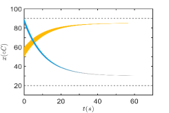
Figure 3. The over-approximate reachable sets for two modes of the heating system. Black dashed lines denote the safety set.

Algorithm 3 presents a procedure to compute a global invariant repeatedly until the safety requirement can be guaranteed by a computed global invariant (when flag holds, line 2-16), then a switching controller solving Problem 1 can be defined by the global invariant (line 17-23). In each iteration, for each mode (line 4-8), we compute a new mode invariant (line 5), a new differential invariant that can guarantee the safety requirement (line 6) by invoking Algorithm 1 (line 8), and a new initial condition satisfying the safety requirement (line 7); for each discrete transition (line 9-12), we compute a new guard condition without considering the discrete delay (line 10), and then a new guard condition considering the discrete delay by calling Algorithm 2 (line 14); then we test whether a global invariant that can guarantee the safety requirement is achieved (line 13-15).

The soundness of our approach is guaranteed by the following theorem.

Theorem 3 (Soundness).

Given a hybrid automaton $\mathcal{H}=(Q,X,U,I,\Xi,F,E,D,G,R)$ and its safety property $\mathcal{S}$, a dHA $\mathcal{H}^{*}=(Q,X,U^{*},I^{*},\Xi^{*},F,E,D,G^{*},R)$ constructed by Algorithm 3 fulfills the three requirements (r1)-r(3) in Problem 1.

Proof.

We first prove that $I^{*}$ is a safe global invariant of $\mathcal{H}^{*}$ if Algorithm 3 terminates and returns $\mathcal{H}^{*}=(Q,X,U^{*},I^{*},\Xi^{*},F,E,$ $D,G^{*},R)$, i.e., the conditions (c1) and (c2) in Definition 2 with restriction of safety requirement $\mathcal{S}$ hold. From line 8 in Algorithm 3, Definition 1 and the soundness of Algorithm 1, we have $I^{*}(q)$ is a safe differential invariant of $(\Xi^{*}(q),f_{q},I(q)$, then (c1) holds. Let $e=(q,q^{\prime})\in E$, and $\bm{\xi}_{\bm{\phi}}^{\mathbf{w}}(t)\in G^{*}(e)$. From line 7, 8 in Algorithm 3, we have

$$\left\{\bm{\phi}\,\middle|\,\begin{array}[]{cc}\exists e=(q^{\prime},q)\in E,\exists t>0,\exists\theta\in[-r_{k}^{q},0].\\ \bm{\phi}=R(e,\mathbf{x}_{t}^{\bm{\phi}}(\cdot))\wedge\mathbf{x}_{t}^{\bm{\phi}}(\theta)\in\widetilde{G}(e)\end{array}\right\}\subseteq I^{*}(q).$$

From line 14, it follows

$$G^{*}_{n}(e)=\textbf{BackReach}(\widetilde{G}_{n}(e),D(e),I_{n}(q),\bm{\rho},\tau),$$

which implies (c2) holds. Now, we prove that (r1), (r2) and (r3) in Problem 1 are satisfied. Since each $I_{n}(q)$ is calculated by Algorithm 1, which can guarantee $I_{n}(q)$ is safe, thus $\mathcal{H}^{*}$ is safe, i.e., (r1) holds. In Algorithm 3, line 9 makes $\Xi^{*}\subseteq\Xi\cap\mathcal{S}$, line 8 makes $I^{*}\subseteq I$. From line 22, and $I^{*}\subseteq I$, it follows $U^{*}\subseteq U$. For any $e\in E$, as there exists $\theta\in[-r^{q}_{k},0]$ such that $\mathbf{x}^{\bm{\phi}}_{t}(\theta)\in G^{*}(e)$, hence $\mathbf{x}^{\bm{\phi}}_{t+D(e)}(\theta)\in\widetilde{G}(e)$. From line 13 and 14, it follows $\mathbf{x}^{\bm{\phi}}_{t+D(e)}(\theta)\in G(e)\cap I^{*}(q)$. Thus, (r2) holds. Clearly, $I^{*}$ contains all safe trajectories of $\mathcal{H}$, so if $\mathcal{H}$ is non-blocking with respect to the safe requirement $\mathcal{S}$, then $\mathcal{H}^{*}$ is also non-blocking, i.e., (r3) holds. ∎

Example 0.

We continue to consider the heating system example. Let $K_{1}=0.25$, $K_{2}=0.15$, $h=32$, $w_{1}=0.5$, and $w_{2}=3$ for the dHA of the heating system in Example 2. For mode $q_{1}$, $M_{q_{1}}=-0.1$ is trivially a Metzler matrix. Applying Theorem 4, we have $T^{*}_{q_{1}}=56.567$s. The same procedure applies to mode $q_{2}$, we have $T^{*}_{q_{2}}=60.043$s. By Algorithm 3, we obtain differential invariants $I^{*}(q_{1})=\{x\mid 30\leq x\leq 84.91\}$ and $I^{*}(q_{2})=\{x\mid 30.2056\leq x\leq 90\}$. Also, strengthened guarded conditions on $e_{1}$ and $e_{2}$ can be easily computed as $G^{*}(e_{1})=\{x\mid 30\leq x\leq 84.30\}$ and $G^{*}(e_{2})=\{x\mid 34.5\leq x\leq 90\}$. The over-approximation of the reachable sets from the initial sets in the two modes respectively are displayed in Figure 3.

Mode	$\epsilon$	$\zeta$	$\beta$	$\eta$	$\gamma$	$\delta$
$q_{1}$	0.001	$\begin{bmatrix}1\\ 1\end{bmatrix}$	1	12.58	5.1642	12.58
$q_{2}$	0.001	$\begin{bmatrix}1\\ 1\end{bmatrix}$	1	24.66	4.2270	24.66

Table 1. The value of parameters in Section 5.1

Mode	$\epsilon$	$\zeta$	$\beta$	$\eta$	$\gamma$	$\delta$	$g_{max}$	$\mathcal{G}$	$\iota$
$q_{1}$	$10^{-4}$	$\begin{bmatrix}1\\ 1\end{bmatrix}$	1	0.8	0.626	0.8	0.008	0.078	0.2
$q_{2}$	$10^{-4}$	$\begin{bmatrix}1\\ 1\end{bmatrix}$	1	1.85	0.88	1.85	0.0046	0.0746	0.2

Table 2. The value of parameters in Section 5.2

5. Experimental Results

We implement our algorithms in Matlab, based upon the interval data-structure in CORA (Althoff and Grebenyuk, 2016). We adopt the discretization parameters from (Althoff and Grebenyuk, 2016) and (Ghafli and Salman, 2020) for the two examples, respectively. All experiments are performed on an Intel(R) Core(TM) i5-8265U CPU (1.60GHz) with 8GB RAM.

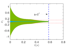
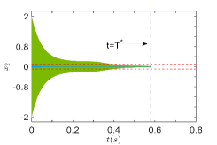
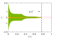
(a)

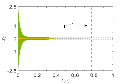
Figure 4. In the low-pass filter system, the over-approximation of the reachable set of mode $q_{1}$ is shown in (a)&(b), and the one of mode $q_{2}$ is shown in (c)&(d). All trajectories, marked with blue for mode $q_{1}$ (yellow for mode $q_{2}$), starting from the states contained in the first ball $\mathfrak{B}(\dfrac{w_{max}}{\delta})$, are always enclosed in the second ball $\mathfrak{B}(\dfrac{w_{max}}{\eta})$ denoted by two red dashed lines.

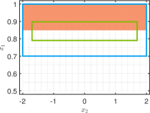
(a) $e_{1}$

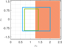
(b) $e_{2}$

Figure 5. The synthesized switching controller on the edge $e_{1}$ and $e_{2}$ of the low-pass filter system. $\widetilde{G}$ is indicated by the blue box, and $G^{*}$ is indicated by the red region. The green box stands for the forward reachable set in $0.01$s from $G^{*}(e_{1})$ ($0.02$s from $G^{*}(e_{2})$).

5.1. Low-pass Filter System

We first consider a low-pass filter system with delays, adapted from CORA (Althoff and Grebenyuk, 2016). It includes two first order low-pass filters $q_{1}$ and $q_{2}$, represented by

$$q_{1}:\left\{\begin{array}[]{lr}\left\{\begin{array}[]{lr}\dot{x}_{1}(t)=-14.58x_{1}(t)+2x_{1}(t-0.1)+0.5\sin(t)\\ \dot{x}_{2}(t)=-20.05x_{2}(t)+2x_{2}(t-0.1)+0.5\sin(t)\end{array}\right.&\\ \Xi(q_{1})=[-1,1]\times[-2,2]&\\ I(q_{1})=\mathbb{R}^{2},&\end{array}\right.$$

$$q_{2}:\left\{\begin{array}[]{lr}\left\{\begin{array}[]{lr}\dot{x}_{1}(t)=-32.66x_{1}(t)+8x_{1}(t-0.1)+0.5\sin(t)\\ \dot{x}_{2}(t)=-47.25x_{2}(t)+8x_{2}(t-0.1)+0.5\sin(t)\end{array}\right.&\\ \Xi(q_{2})=[-2.25,2.5]\times[-2.5,2.5]&\\ I(q_{2})=\mathbb{R}^{2}.&\end{array}\right.$$

There are two discrete transitions $e_{1}=(q_{1},q_{2})$ and $e_{2}=(q_{2},q_{1})$ between $q_{1}$ and $q_{2}$, and the corresponding guard conditions are $G(e_{1})=\{(x_{1},x_{2})\in\mathbb{R}^{2}\mid x_{1}\geq 0.7\}$, $G(e_{2})=\{(x_{1},x_{2})\in\mathbb{R}^{2}\mid x_{2}\geq 0.6\}$. Reset functions are identity mappings. Moreover, both discrete transitions are taken with delays $D(e_{1})=0.02$ and $D(e_{2})=0.02$, respectively. The safety requirement is $\mathcal{S}=\{(x_{1},x_{2})\in\mathbb{R}^{2}\mid-2.7\leq x_{1}\leq 2.7\wedge-2.6\leq x_{2}\leq 2.6\}$.

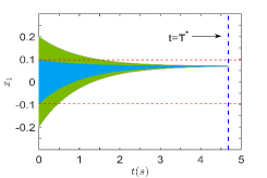
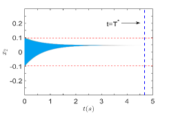
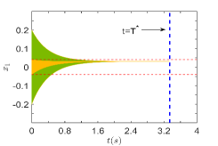
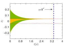
Figure 6. In the predator-prey populations system, the over-approximation of the reachable set of mode $q_{1}$ is shown in (a)&(b), and the one of mode $q_{2}$ is shown in (c)&(d). All trajectories, marked with blue for mode $q_{1}$ (yellow for mode $q_{2}$), starting from the states contained in the first ball $\mathfrak{B}(\dfrac{\mathcal{G}}{\delta})$, are always enclosed in the second ball $\mathfrak{B}(\dfrac{\mathcal{G}}{\eta})$ denoted by two red dashed lines.

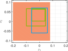
(a) $e_{1}$

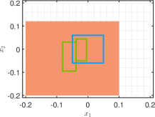
(b) $e_{2}$

Figure 7. The synthesized switching controllers on the edge $e_{1}$ and $e_{2}$ of the predator-prey population system. $\widetilde{G}$ is indicated by the blue box, and $G^{*}$ by the red region. The green boxes stand for the over-approximation of the reachable sets in $0.5$s and $0.8$s from $G^{*}(e_{1})$ (in $0.3$s and $0.5$s from $G^{*}(e_{2})$), respectively.

For mode $q_{1}$, $M_{q_{1}}=\begin{bmatrix}-12.58&0\\ 0&-18.05\end{bmatrix}$ is obviously a Metzler matrix satisfying the two properties listed in Proposition 2. By Theorem 4, the differential invariant synthesis problem is reduced to a $T^{*}_{q_{1}}$-differential invariant synthesis problem, where $T^{*}_{q_{1}}=0.5782s$ is computed with the parameters listed in Table 2. Similarly, for mode $q_{2}$, $M_{q_{2}}=\begin{bmatrix}-4.66&0\\ 0&-39.25\end{bmatrix}$ is also a Metzler matrix satisfying the two properties listed in Proposition 2. $T^{*}_{q_{2}}=0.7605s$ is computed with the parameters listed in Table 2. The computed over-approximation of the reachable set within $T^{*}_{q_{1}}$ for mode $q_{1}$ using our approach is given in Fig. 4 and 4. The over-approximation of the reachable set in $T^{*}_{q_{2}}$ for mode $q_{2}$ is shown in Figure 4(a) and 4 with our approach. Clearly, the delay dynamical system in this mode satisfies the ball convergence property. The guard conditions without discrete delays are $\widetilde{G}(e_{1})=\{(x_{1},x_{2})\in\mathbb{R}^{2}\mid 0.7\leq x_{1}\leq 1\wedge-2\leq x_{2}\leq 2\}$ and $\widetilde{G}(e_{2})=\{(x_{1},x_{2})\in\mathbb{R}^{2}\mid-1\leq x_{1}\leq 1\wedge 0.6\leq x_{2}\leq 2\}$. Finally, applying Algorithm 2, the strengthened guard conditions $G^{*}(e_{1})$ and $G^{*}(e_{2})$, that can guarantee the safety, are computed as showed in Fig. 5.

5.2. Predator-prey Populations

We consider a nonlinear predator-prey population dynamics under seasonal succession: a hybrid Lotka–Volterra competition model with delays adapted from (Li et al., 2017). Two modes for two seasons are modelled as follows:

$$q_{1}:\left\{\begin{array}[]{lr}\left\{\begin{array}[]{lr}\dot{x}_{1}(t)=-x_{1}(t)(1-\frac{x_{1}(t)}{100})+0.2d_{1}+w_{11}(t)\\ \dot{x}_{2}(t)=-1.5x_{2}(t)(1-\frac{x_{2}(t)}{100})+0.1d_{2}+w_{12}(t)\end{array}\right.&\\ \Xi(q_{1})=[-0.2,0.2]\times[-0.1,0.1]&\\ I(q_{1})=\mathbb{R}^{2}.&\end{array}\right.\\$$

$$q_{2}:\left\{\begin{array}[]{lr}\left\{\begin{array}[]{lr}\dot{x}_{1}(t)=-2.5x_{1}(t)+0.2x_{1}(t-0.01)(1+x_{2}(t))+w_{21}(t)\\ \dot{x}_{2}(t)=-2x_{2}(t)+0.15x_{2}(t-0.01)(1+x_{2}(t))+w_{22}(t)\end{array}\right.&\\ \Xi(q_{2})=[-0.2,0.2]\times[-0.2,0.2]&\\ I(q_{2})=\mathbb{R}^{2}.&\end{array}\right.$$

where $q_{1}$ and $q_{2}$ represent two seasons, $d_{1}=x_{1}(t-0.1)(1+x_{1}(t))$, $d_{2}=x_{2}(t-0.1)(1+x_{2}(t))$, $x_{1}$ is the number of prey (for example, rabbits), $x_{2}$ is the number of some predator (for example, foxes), $w_{ij}(t)=0.07\cos{2t}$ ($i,j=1,2$) denote the perturbations. The real coefficients describe the interaction of the two species, the intrinsic growth rate and the environment capacity of the population in season $i$, respectively. There are two discrete transitions $e_{1}=(q_{1},q_{2})$ and $e_{2}=(q_{2},q_{1})$ between mode $q_{1}$ and mode $q_{2}$, and their corresponding guard conditions initially are $G(e_{1})=\{(x_{1},x_{2})\in\mathbb{R}^{2}\mid-0.06\leq x_{1}\leq 0.06\wedge-0.06\leq x_{2}\leq 0.07\}$, $G(e_{2})=\{(x_{1},x_{2})\in\mathbb{R}^{2}\mid-0.05\leq x_{1}\leq 0.05\wedge-0.06\leq x_{2}\leq 0.06\}$. Reset functions are identity mappings. Moreover, both discrete transitions are taken with delays $D(e_{1})=1$ and $D(e_{2})=0.55$, respectively. The safety requirement is $\mathcal{S}=\{(x_{1},x_{2})\in\mathbb{R}^{2}\mid-0.20\leq x_{1}\leq 0.21\wedge-0.21\leq x_{2}\leq 0.22\}$.

By linearizing mode $q_{1}$, we have:

$$\left\{\begin{array}[]{lr}\dot{x}_{1}(t)=-x_{1}(t)+0.2x_{1}(x-0.1)+w_{11}(t)\\ \dot{x}_{2}(t)=-1.5x_{2}(t)+0.1x_{2}(x-0.1)+w_{12}(t)\end{array}\right..$$

Clearly, $M_{q_{1}}=\begin{bmatrix}-0.8&0\\ 0&-1.4\end{bmatrix}$ is a Metzler matrix satisfying the two properties listed in Proposition 2. By Theorems 10 and 11, the differential invariant synthesis problem for mode $q_{1}$ is reduce to a $T^{*}_{q_{1}}$-differential invariant synthesis problem, where $T^{*}_{q_{1}}=4.6825$s is computed using our approach with the parameters listed in Table 2.

Here it is noteworthy that $\iota=0.2$, covering the entire initial set. Similarly, for mode $q_{2}$, the linearization of its dynamics is :

$$\left\{\begin{array}[]{lr}\dot{x}_{1}(t)=-2.5x_{1}(t)+0.2x_{1}(t-0.01)+w_{21}(t)\\ \dot{x}_{2}(t)=-2x_{2}(t)+0.15x_{2}(t-0.01)+w_{22}(t)\end{array}\right..$$

Clearly, $M_{q_{2}}=\begin{bmatrix}-2.3&0\\ 0&-1.85\end{bmatrix}$ is also a Metzler matrix satisfying the two properties listed in Proposition 2. With the parameters listed in Table 2, a bounded time $T^{*}_{q_{2}}=3.3326$s is computed. The computed over-approximation of the reachable set within $t\geq T^{*}_{q_{1}}$ for mode $q_{1}$ is showed in Fig. 6&6. And the computed over-approximation of the reachable set within $t\geq T^{*}_{q_{2}}$ for mode $q_{2}$ are shown in Fig. 6&6 using our approach. The guard conditions without discrete delays are computed as $\widetilde{G}(e_{1})=\{(x_{1},x_{2})\in\mathbb{R}^{2}\mid-0.06\leq x_{1}\leq 0.06\wedge-0.06\leq x_{2}\leq 0.07\}$ and $\widetilde{G}(e_{2})=\{(x_{1},x_{2})\in\mathbb{R}^{2}\mid-0.05\leq x_{1}\leq 0.05\wedge-0.06\leq x_{2}\leq 0.06\}$. Finally, applying Algorithm 2, the strengthened guard conditions $G^{*}(e_{1})$ and $G^{*}(e_{2})$, which can guarantee the safety requirement, are obtained as shown in Fig. 7.

6. Conclusion

We introduced the notion of delay hybrid automata (dHA) in order to model continuous delays and discrete delays in cyber-physical systems uniformly. Based on dHA, we proposed an approach on how to automatically synthesize a switching controller for a delay hybrid system with perturbations against a given safety requirement. To the end, we presented a new approach for over-approximating a nonlinear DDE with perturbation using ball-convergence analysis based on Metzler matrix. Two case studies were provided to indicate the effectiveness and efficiency of the proposed approach.

For future work, it deserves to investigate how to synthesize a switching controller for a dHA against much richer properties defined e.g. by signal temporal logic (Maler and Nickovic, 2004) or metric temporal logic (Koymans, 1990). In addition, it is interesting to consider our method to deal with more general forms of DDEs. Besides, it is a challenge how to guarantee the completeness of our approach, which essentially corresponds to a long-standing problem on how to compute reachable sets of hybrid systems in the infinite time horizon.

References

- (1)
- Althoff and Grebenyuk (2016) M. Althoff and D. Grebenyuk. 2016. Implementation of Interval Arithmetic in CORA 2016. In Proc. of the 3rd International Workshop on Applied Verification for Continuous and Hybrid Systems.
- Alur et al. (1995) R. Alur, C. Courcoubetis, N. Halbwachs, T.A. Henzinger, P.-H. Ho, X. Nicollin, A. Olivero, J. Sifakis, and S. Yovine. 1995. The algorithmic analysis of hybrid systems. Theoretical Computer Science 138, 1 (1995), 3 – 34. https://doi.org/10.1016/0304-3975(94)00202-T Hybrid Systems.
- Asarin et al. (2000) E. Asarin, O. Bournez, T. Dang, O. Maler, and A. Pnueli. 2000. Effective synthesis of switching controllers for linear systems. Proc. IEEE 88, 7 (2000), 1011–1025.
- Bai et al. (2021) Yunjun Bai, Ting Gan, Li Jiao, Bai Xue, and Naijun Zhan. 2021. Switching Controller Synthesis for Time-delayed Hybrid Systems. Science China Mathematica 51, 1(1-2) (2021), 97–114. in Chinese.
- Belta et al. (2017) C. Belta, B. Yordanov, and E. Aydin Gol. 2017. Formal Methods for Discrete-Time Dynamical Systems. Springer.
- Berman and Plemmons (1994) Abraham Berman and Robert J Plemmons. 1994. Nonnegative matrices in the mathematical sciences. Vol. 9. Siam.
- Chen et al. (2020) Mingshuai Chen, Martin Fraenzle, Yangjia Li, Peter N. Mosaad, and Naijun Zhan. 2020. Indecision and delays are the parents of failure – Taming them algorithmically by synthesizing delay-resilient control. Acta Informatica (2020). https://doi.org/10.1007/s00236-020-00374-7
- Chen et al. (2016) M. Chen, M. Fränzle, Y. Li, P. Mosaad, and N. Zhan. 2016. Validated Simulation-Based Verification of Delayed Differential Dynamics. In FM 2016 (LNCS), Vol. 9995. 137–154.
- Chen et al. (2018) Mingshuai Chen, Martin Fränzle, Yangjia Li, Peter Nazier Mosaad, and Naijun Zhan. 2018. What’s to Come is Still Unsure - Synthesizing Controllers Resilient to Delayed Interaction. In ATVA 2018 (LNCS), Vol. 11138. 56–74.
- Feng et al. (2019) Shenghua Feng, Mingshuai Chen, Naijun Zhan, Martin Fränzle, and Bai Xue. 2019. Taming Delays in Dynamical Systems. In CAV 2019 (LNCS), Vol. 11561. Springer, 650–669.
- Ghafli and Salman (2020) Ahmed A. Al Ghafli and Hassan J. Al Salman. 2020. An optimal error bound for a finite element approximation of spatially extended predator-prey interaction model. Numerical Algorithms 85, 1 (2020), 209–229. https://doi.org/10.1007/s11075-019-00810-x
- Girard (2012) Antoine Girard. 2012. Controller synthesis for safety and reachability via approximate bisimulation. Automatica 48, 5 (2012), 947–953.
- Goubault and Putot (2019) Eric Goubault and Sylvie Putot. 2019. Inner and outer reachability for the verification of control systems.. In HSCC. 11–22.
- Henzinger et al. (1995) Thomas A Henzinger, Peter W Kopke, Anuj Puri, and Pravin Varaiya. 1995. What’s decidable about hybrid automata? Technical Report. Cornell University.
- Hien and Trinh (2014) Le Van Hien and Hieu Minh Trinh. 2014. A new approach to state bounding for linear time-varying systems with delay and bounded disturbances. Automatica 50, 6 (2014), 1735 – 1738. https://doi.org/10.1016/j.automatica.2014.04.025
- Hsu et al. (2018) K. Hsu, R. Majumdar, K. Mallik, and A.-K. Schmuck. 2018. Multi-Layered Abstraction-Based Controller Synthesis for Continuous-Time Systems. In HSCC’18. ACM, 120–129.
- Huang et al. (2017) Zhenqi Huang, Chuchu Fan, and Sayan Mitra. 2017. Bounded invariant verification for time-delayed nonlinear networked dynamical systems. Nonlinear Analysis: Hybrid Systems 23 (2017), 211–229.
- Jha et al. (2011) S. Jha, S. A. Seshia, and A. Tiwari. 2011. Synthesis of optimal switching logic for hybrid systems. In EMSOFT 2011. 107–116.
- Kong et al. (2015) Soonho Kong, Sicun Gao, Wei Chen, and Edmund M. Clarke. 2015. dReach: -Reachability Analysis for Hybrid Systems. In TACAS 2015 (LNCS), Christel Baier and Cesare Tinelli (Eds.), Vol. 9035. Springer, 200–205.
- Koymans (1990) Ron Koymans. 1990. Specifying Real-Time Properties with Metric Temporal Logic. Real Time Syst. 2, 4 (1990), 255–299.
- Li et al. (2017) Yanqing. Li, Long. Zhang, and Zhidong. Teng. 2017. Single-species model under seasonal succession alternating between Gompertz and Logistic growth and impulsive perturbations. GEM - International Journal on Geomathematics 8, 6 (2017), 241––260. https://doi.org/10.1007/s13137-017-0092-9
- Lyapunov (1992) A. M. Lyapunov. 1992. The general problem of the stability of motion. Internat. J. Control 55, 3 (1992), 531–534. https://doi.org/10.1080/00207179208934253
- Maler and Nickovic (2004) Oded Maler and Dejan Nickovic. 2004. Monitoring Temporal Properties of Continuous Signals. In FORMATS 2004 + FTRTFT (LNCS), Yassine Lakhnech and Sergio Yovine (Eds.), Vol. 3253. Springer, 152–166.
- Nilsson et al. (2017) Petter Nilsson, Necmiye Ozay, and Jun Liu. 2017. Augmented finite transition systems as abstractions for control synthesis. Discrete Event Dynamic Systems 27, 2 (2017), 301–340.
- Pola et al. (2015) Giordano Pola, Pierdomenico Pepe, and Maria Domenica Di Benedetto. 2015. Symbolic models for time-varying time-delay systems via alternating approximate bisimulation. International Journal of Robust and Nonlinear Control 25, 14 (2015), 2328–2347.
- Pola et al. (2010) Giordano Pola, Pierdomenico Pepe, Maria D Di Benedetto, and Paulo Tabuada. 2010. Symbolic models for nonlinear time-delay systems using approximate bisimulations. Systems & Control Letters 59, 6 (2010), 365–373.
- Prajna and Jadbabaie (2005) S. Prajna and A. Jadbabaie. 2005. Methods for safety verification of time-delay systems. In CDC 2005. 4348–4353.
- P.Tabuada (2009) P.Tabuada. 2009. Verification and control of hybrid systems: a symbolic approach. Springer.
- Reissig et al. (2017) G. Reissig, A. Weber, and M. Rungger. 2017. Feedback Refinement Relations for the Synthesis of Symbolic Controllers. IEEE Trans. Automat. Control 62, 4 (2017), 1781–1796.
- Richard Kicsinya (2012) Farkasb Richard Kicsinya. 2012. Improved differential control for solar heating systems. Solar Energy 86, 11 (2012), 3489–3498.
- Taly and Tiwari (2010) Ankur Taly and Ashish Tiwari. 2010. Switching logic synthesis for reachability. In EMSOFT 2010. ACM, 19–28.
- Tomlin et al. (2000) C. J. Tomlin, J. Lygeros, and S. Shankar Sastry. 2000. A game theoretic approach to controller design for hybrid systems. Proc. IEEE 88, 7 (2000), 949–970.
- Xue et al. (2017) Bai Xue, Peter Nazier Mosaad, Martin Fränzle, Mingshuai Chen, Yangjia Li, and Naijun Zhan. 2017. Safe over-and under-approximation of reachable sets for delay Differential equations. In FORMATS 2017 (LNCS), Vol. 10419. Springer, 281–299.
- Xue et al. (2021) Bai Xue, Qiuye Wang, Shenghua Feng, and Naijun Zhan. 2021. Over- and Under-Approximating Reachable Sets for Perturbed Delay Differential Equations. IEEE Trans. Automat. Control 66, 1 (2021), 283–290.
- Zhao et al. (2013) Hengjun Zhao, Naijun Zhan, and Deepak Kapur. 2013. Synthesizing switching controllers for hybrid systems by generating invariants. In Theories of Programming and Formal Methods. Springer, 354–373.
- Zou et al. (2015) L. Zou, M. Fränzle, N. Zhan, and P. Mosaad. 2015. Automatic Verification of Stability and Safety for Delay Differential Equations. In CAV 2015 (LNCS), Vol. 9207. 338–355.