Metastability of Blume–Capel Model with Zero Chemical Potential and Zero External Field

Abstract.

In this study, we investigate the metastable behavior of Metropolis-type Glauber dynamics associated with the Blume–Capel model with zero chemical potential and zero external field at very low temperatures. The corresponding analyses for the same model with zero chemical potential and positive small external field were performed in [Cirillo and Nardi, Journal of Statistical Physics, 150: 1080-1114, 2013] and [Landim and Lemire, Journal of Statistical Physics, 164: 346-376, 2016]. We obtain both large deviation-type and potential-theoretic results on the metastable behavior in our setting. To this end, we perform highly thorough investigation on the energy landscape, where it is revealed that no critical configurations exist and alternatively a massive flat plateau of saddle configurations resides therein.

1. Introduction

Within the context of statistical mechanics, metastability is a phenomenon of first-order phase transition that occurs in various systems consisting of multiple locally stable states. Extensive research has been carried out on metastability since the mid-20th century, ranging from the early works [6, 7] to recently developed methodologies [1, 2, 3, 17]. As a result, various stochastic systems have been known to exhibit such behavior; important examples include the small random perturbations of dynamical systems [6, 18, 25], condensing interacting particle systems [12, 13, 17, 26], and ferromagnetic spin systems at low temperatures [4, 10, 15, 16, 21, 23]. We refer to the classic monographs [5, 24] for detailed explanation on the history and perspectives regarding the phenomenon of metastability.

We investigate the metastable behavior of the well-known Blume–Capel model on two-dimensional (2D) lattices. This model is a ferromagnetic spin system that consists of three spins, namely $-1$, $0$, and $+1$, and it was originally introduced to study the ${}^{3}\mathrm{He}$–${}^{4}\mathrm{He}$ phase transition. In this system, spin $0$ at a site indicates the absence of particles, whereas spin $-1$ (resp. $+1$) at a site means that the site is occupied by a particle with spin $-1$ (resp. $+1$). The system is controlled by the Hamiltonian function (cf. (2.2)) that is defined on the collection of spin configurations. This Hamiltonian represents the ferromagnetic behavior of the spins in the sense that more aligned spin configurations exhibit greater stability. Thus, the most stable configurations are the monochromatic ones (cf. (2.5)). The system is controlled by Metropolis-type Glauber dynamics (cf. (2.7)), where $\beta$ is the inverse temperature, so that it becomes exponentially difficult to overcome the energy barrier in each spin update. According to the dynamics, we investigate the long-time metastable transitions between the monochromatic spin configurations in the low-temperature regime $\beta\rightarrow\infty$.

An inspection of formula (2.2) reveals that the Hamiltonian has two variables: the chemical potential $\lambda$ and external magnetic field $h$. We are interested in the metastable behavior when these external effects are small; that is, when $(\lambda,\,h)$ is close to $(0,\,0)$. The case of $0<|\lambda|<h$ was thoroughly investigated in [10, 20], where [10] worked on fixed finite square tori and [20] worked on the infinite lattice $\mathbb{Z}^{2}$. Subsequently, the case of $\lambda=0$ and $h>0$ was studied in [8, 9, 15, 16], where [8, 9, 15] considered fixed finite square tori and [16] considered finite square tori whose lengths increase to infinity. In all of the above works, the authors established the existence of a special form of critical saddle configurations, whereby the metastable transitions between the monochromatic configurations must pass through a configuration of this type.

In this study, we investigate the Blume–Capel model on fixed finite lattices in the case of $\lambda=h=0$, in which it is remarkable that no critical saddle configurations exist. Instead, a metastable transition starting from a monochromatic configuration must occur along a massive flat plateau of saddle configurations to reach another. Hence, to analyze the exact behavior of the metastable transitions quantitatively, the overall energy landscape of spin configurations in the system must be investigated. This is the main mathematical obstacle that is successfully overcome in the current study.

The massive flat saddle plateau is indeed the essence of the energy landscape in our model. We denote by typical configurations (cf. Definition 5.1) those that are reachable by metastable transitions with respect to the correct scale. Then, we obtain two types of typical configurations, namely bulk ones and edge ones. Bulk typical configurations form the main component of metastable transitions and their structure is very simple in that the transitions occur one-dimensionally therein. Edge typical configurations constitute the initiating and finalizing components of metastable transitions and their structure is complex compared to that of the bulk ones. Hence, the edge typical configurations need to be handled much more delicately, as described in Section 6.

The structure of edge typical configurations is strongly dependent on the boundary conditions on the lattice. More specifically, if the lattice has open boundaries (i.e., $\Lambda=\llbracket 1,\,K\rrbracket\times\llbracket 1,\,L\rrbracket\subseteq\mathbb{Z}^{2}$), the structure is relatively simple and the exact behavior of the dynamics can be computed. However, if the lattice has periodic boundaries (i.e., $\Lambda=\mathbb{T}_{K}\times\mathbb{T}_{L}$), the situation becomes complex and the structure becomes a Markov chain on certain subtrees of a $K\times 2$-shaped ladder graph. Although we cannot characterize the exact behavior of the dynamics in this case, our estimate is sufficient to deduce the main results of this study. We refer to Remarks 2.6, 2.10, and A.2 for further details.

The main results obtained in this study are divided into two types: large deviation-type results (cf. Section 2.2) and potential theory-type results (cf. Section 2.3). For the former, we use the pathwise approach [7] to metastability; in particular, the recent methodology [22], which enables us to estimate certain concepts regarding metastability (the transition time, mixing time, and spectral gap) by analyzing the valley depths of the energy landscape. For the latter, we use the potential-theoretic [6] and martingale [1, 2, 3] approaches to metastability. These methods offer the advantage of providing the sharp asymptotics of the transition time by analyzing the capacity (cf. (3.4)), which is unattainable with the classic pathwise approach to metastability.

The Blume–Capel model has many similar features to the stochastic Potts model with three spins, which generalizes the number of spins of the well-known stochastic Ising model (which has two spins, $-1$ and $+1$). The metastable behavior of the Ising and Potts models has been studied extensively in the past several decades [4, 21, 23]. Recently, we conducted in [14] (which is our companion paper) a quantitative analysis on the metastable behavior of the Ising and Potts models with zero external fields on two- and three- dimensional lattices, and we frequently refer to [14] for insights into and details on the deductions presented in this article.

Natural open questions arise in two directions. The first objective is to investigate the dynamics with $\lambda=h=0$ on growing lattices, as demonstrated by the authors of [16] for the case of $\lambda=0$ and $h>0$. In this case, the growth rate of the lattice and transition rate between the saddle configurations need to be compared to deduce the exact time scale. The second objective is to study the dynamics with $\lambda=h=0$ in the infinite volume lattice, as accomplished in [20], for which it is necessary to investigate whether a specific form of critical configurations still fails to exist in the infinite volume case or emerges in this particular setting.

2. Main Results

2.1. Model definition

Blume–Capel model

We define the Blume–Capel model on the finite 2D lattice box $\Lambda=\llbracket 1,\,K\rrbracket\times\llbracket 1,\,L\rrbracket$, where $K$ and $L$ are fixed positive integers. For convenience, we assume that

$$5\leq K\leq L.$$ (2.1)

We impose either open or periodic boundary conditions on $\Lambda$. If $K=L$ under the periodic boundary conditions, the lattice is indeed $\mathbb{T}_{L}\times\mathbb{T}_{L}$ as in the previous studies [8, 9, 15]. For $x,\,y\in\Lambda$, we write $x\sim y$ if they are nearest neighbors; that is, $|x-y|=1$.

We have three spins in this model, namely $-1$, $0$, and $+1$. We denote by $\mathcal{X}=\{-1,\,0,\,+1\}^{\Lambda}$ the space of the spin configurations on $\Lambda$. Subsequently, we define the Hamiltonian $H:\mathcal{X}\rightarrow\mathbb{R}$ as

$$H(\sigma)=\sum_{x\sim y}\{\sigma(x)-\sigma(y)\}^{2}-\lambda\sum_{x\in\Lambda}\sigma(x)^{2}-h\sum_{x\in\Lambda}\sigma(x).$$ (2.2)

Here, $\sigma(x)$ is the spin of configuration $\sigma\in\mathcal{X}$ at site $x\in\Lambda$. Moreover, we assume that the chemical potential $\lambda$ and external field $h$ are both zero, so that

$$H(\sigma)=\sum_{x\sim y}\{\sigma(x)-\sigma(y)\}^{2}.$$ (2.3)

We denote by $\mu_{\beta}$ the Gibbs measure on $\mathcal{X}$ associated with the Hamiltonian $H$ at the inverse temperature $\beta>0$:

$$\mu_{\beta}(\sigma)=\frac{1}{Z_{\beta}}e^{-\beta H(\sigma)},\;\;\;\;Z_{\beta}=\sum_{\sigma\in\mathcal{X}}e^{-\beta H(\sigma)}.$$ (2.4)

We denote by $\mathbf{-1},\,\mathbf{0},\,\mathbf{+1}\in\mathcal{X}$ the monochromatic configurations, of which all spins are $-1,\,0,\,+1$, respectively. We write

$$\mathcal{S}=\{\mathbf{-1},\,\mathbf{0},\,\mathbf{+1}\}.$$ (2.5)

When we select spins $a$ or $b$, the corresponding monochromatic configuration is denoted by $\mathbf{a}\in\mathcal{S}$ or $\mathbf{b}\in\mathcal{S}$, respectively. It is precisely on $\mathcal{S}$ that $H(\cdot)$ attains its minimum $0$, and hence, $\mathcal{S}$ denotes the collection of ground states. The following estimates are straightforward:

$$Z_{\beta}=3+O(e^{-2\beta})\;\;\;\;\text{and}\;\;\;\;\lim_{\beta\rightarrow\infty}\mu_{\beta}(\mathbf{s})=\frac{1}{3}\text{ for all }\mathbf{s}\in\mathcal{S}.$$ (2.6)

Continuous-time Metropolis dynamics

For $\sigma\in\mathcal{X}$, $x\in\Lambda$, and spin $a$, we denote by $\sigma^{x,a}\in\mathcal{X}$ the configuration obtained from $\sigma$ by updating the spin at site $x$ to $a$. Thereafter, the dynamics is defined as the continuous-time Markov chain $\{\sigma_{\beta}(t)\}_{t\geq 0}$ on $\mathcal{X}$, the transition rates of which are given by

$$c_{\beta}(\sigma,\,\zeta)=\begin{cases}e^{-\beta[H(\zeta)-H(\sigma)]_{+}}&\text{if }\zeta=\sigma^{x,a}\neq\sigma\text{ for some }x\in\Lambda\text{ and spin }a,\\ 0&\text{otherwise},\end{cases}$$ (2.7)

where $[t]_{+}=\max\{t,\,0\}$. It is easy to observe that $\sigma_{\beta}(\cdot)$ is irreducible. For $\sigma,\,\zeta\in\mathcal{X}$, we write $\sigma\sim\zeta$ if $c_{\beta}(\sigma,\,\zeta)>0$. It is clear that $\sigma\sim\zeta$ if and only if $\zeta\sim\sigma$, and that the relation $\sigma\sim\zeta$ does not depend on the exact value of $\beta>0$. Moreover, for each $\mathcal{A}\subseteq\mathcal{X}$, we define the collection of edges in $\mathcal{A}$ as follows:

$$E(\mathcal{A})=\{\{\sigma,\,\zeta\}\subseteq\mathcal{A}:\sigma\sim\zeta\}.$$ (2.8)

For the above dynamics, the detailed balance condition holds; that is,

$$\mu_{\beta}(\sigma)c_{\beta}(\sigma,\,\zeta)=\mu_{\beta}(\zeta)c_{\beta}(\zeta,\,\sigma)=\begin{cases}\min\{\mu_{\beta}(\sigma),\,\mu_{\beta}(\zeta)\}&\text{if }\sigma\sim\zeta,\\ 0&\text{otherwise}.\end{cases}$$ (2.9)

Hence, the invariant measure of this Metropolis dynamics $\sigma_{\beta}(\cdot)$ is exactly $\mu_{\beta}$, and $\sigma_{\beta}(\cdot)$ is reversible with respect to $\mu_{\beta}$. We denote by $\mathbb{P}_{\sigma}^{\beta}$ and $\mathbb{E}_{\sigma}^{\beta}$ the law and expectation, respectively, of the process $\sigma_{\beta}(\cdot)$ starting from $\sigma\in\mathcal{X}$.

Remark 2.1.

We remark on the model symmetry. First, our model is fully symmetric with respect to the spin correspondence $-1\leftrightarrow+1$. However, our model is not symmetric with respect to $-1\leftrightarrow 0$ or $0\leftrightarrow+1$. Therefore, spins $-1$ and $+1$ play the same role, but spin $0$ does not. This is the main difference from the Potts model studied in [14, 21], in which all of the spins play the same role. More specifically, we present the following differentiated features in this study:

• The canonical transitions occur only along good pairs of spins (cf. Notation 4.1). Thus, when analyzing the relevant configurations, care should be taken with this underlying asymmetry of the model.

• The typical configurations are defined individually for each good pair, whereas the corresponding ones are globally defined in [14]. This is because the edge typical configurations near $\mathbf{-1}$ and $\mathbf{+1}$ possess a different structure compared to those near $\mathbf{0}$ (cf. Section 6; see also Remark 6.1).

• We cannot estimate the capacities in a unified manner owing to the model asymmetry; thus, we first construct fundamental test functions and flows in Section 7, which serve as the building blocks for the actual test objects. Subsequently, in Section 8, we construct individual test objects for each capacity (cf. Theorem 3.3).

2.2. Main results: large deviation-type results

In this subsection, we explain the large deviation-type main results on the metastable behavior.

Energy barrier between ground states

First, we introduce the energy barrier of the energy landscape, which is the level of energy that must be overcome to enable a metastable transition from one ground state to another.

Definition 2.2.

We define the following objects:

1. A sequence of configurations $(\omega_{n})_{n=0}^{N}=(\omega_{0},\,\omega_{1},\,\dots,\,\omega_{n})\subseteq\mathcal{X}$ is called a path if $\omega_{n}\sim\omega_{n+1}$ for all $n\in\llbracket 0,\,N-1\rrbracket$. We state that this path connects $\sigma$ and $\zeta$ if $\omega_{0}=\sigma$ and $\omega_{N}=\zeta$, or vice versa. Moreover, we state that this path is in $\mathcal{A}\subseteq\mathcal{X}$ if $\omega_{n}\in\mathcal{A}$ for all $n\in\llbracket 0,\,N\rrbracket$. For $c\in\mathbb{R}$, a path $(\omega_{n})_{n=0}^{N}$ is called a $c$-path if $H(\omega_{n})\leq c$ for all $n\in\llbracket 0,\,N\rrbracket$.

2. The communication height between two configurations $\sigma,\,\zeta\in\mathcal{X}$ is defined by

   $$\Phi(\sigma,\,\zeta)=\min_{(\omega_{n})_{n=0}^{N}}\max_{n\in\llbracket 0,N\rrbracket}H(\omega_{n}),$$

   where the minimum is taken over all paths $(\omega_{n})_{n=0}^{N}$ that connect $\sigma$ and $\zeta$. Furthermore, the communication height between two disjoint sets $\mathcal{A},\,\mathcal{B}\subseteq\mathcal{X}$ is defined by

   $$\Phi(\mathcal{A},\,\mathcal{B})=\min_{\sigma\in\mathcal{A}}\min_{\zeta\in\mathcal{B}}\Phi(\sigma,\,\zeta).$$

3. For two spins $a$ and $b$, we define the energy barrier between $\mathbf{a},\,\mathbf{b}\in\mathcal{S}$ by

   $$\Gamma_{a,b}=\Gamma_{a,b}(K,\,L)=\Phi(\mathbf{a},\,\mathbf{b}).$$ (2.10)

   It is clear that $\Gamma_{a,b}=\Gamma_{b,a}$.

The following theorem characterizes the exact energy barrier; we recall (2.1).

Theorem 2.3 (Energy barrier).

Define a constant $\Gamma$ by

$$\Gamma=\begin{cases}2K+2&\text{under periodic boundary conditions},\\ K+1&\text{under open boundary conditions}.\end{cases}$$ (2.11)

Then, it holds that

$$\Gamma_{-1,0}=\Gamma_{0,+1}=\Gamma_{-1,+1}=\Gamma.$$ (2.12)

The proof of Theorem 2.3 is provided in Section 4.2.

Large deviation-type results

We first define the following concepts:

• For $\mathcal{A}\subseteq\mathcal{X}$, we denote by $\tau_{\mathcal{A}}$ the hitting time of the set $\mathcal{A}$. Subsequently, for $\mathbf{s}\in\mathcal{S}$, the hitting times $\tau_{\mathcal{S}\setminus\{\mathbf{s}\}}$ and $\tau_{\mathbf{s}^{\prime}}$, $\mathbf{s}^{\prime}\in\mathcal{S}\setminus\{\mathbf{s}\}$ are called the (metastable) transition times starting from $\mathbf{s}$.

• The mixing time with respect to $\epsilon\in(0,\,1)$ is defined by

  $$t_{\beta}^{\mathrm{mix}}(\epsilon)=\min\big{\{}t\geq 0:\max_{\sigma\in\mathcal{X}}\|\mathbb{P}_{\sigma}^{\beta}[\sigma_{\beta}(t)\in\cdot]-\mu_{\beta}(\cdot)\|_{\mathrm{TV}}\leq\epsilon\big{\}},$$

  where $\|\cdot\|_{\mathrm{TV}}$ denotes the total variation distance (cf. [19, Chapter 4]).

• We denote by $\lambda_{\beta}$ the spectral gap of our dynamics (cf. [19, Chapter 12]).

Theorem 2.4 (Large deviation-type results).

The following statements hold.

1. (Transition time) For all $\mathbf{s},\,\mathbf{s}^{\prime}\in\mathcal{S}$ and $\epsilon>0$, we have

   $$\lim_{\beta\rightarrow\infty}\mathbb{P}_{\mathbf{s}}^{\beta}[e^{\beta(\Gamma-\epsilon)}<\tau_{\mathcal{S}\setminus\{\mathbf{s}\}}\leq\tau_{\mathbf{s}^{\prime}}<e^{\beta(\Gamma+\epsilon)}]=1,$$ (2.13)

   $$\lim_{\beta\rightarrow\infty}\frac{1}{\beta}\log\mathbb{E}_{\mathbf{s}}^{\beta}[\tau_{\mathcal{S}\setminus\{\mathbf{s}\}}]=\lim_{\beta\rightarrow\infty}\frac{1}{\beta}\log\mathbb{E}_{\mathbf{s}}^{\beta}[\tau_{\mathbf{s}^{\prime}}]=\Gamma.$$ (2.14)

   Moreover, under $\mathbb{P}_{\mathbf{s}}^{\beta}$, as $\beta\rightarrow\infty$,

   $$\frac{\tau_{\mathcal{S}\setminus\{\mathbf{s}\}}}{\mathbb{E}_{\mathbf{s}}^{\beta}[\tau_{\mathcal{S}\setminus\{\mathbf{s}\}}]}\rightharpoonup\mathrm{Exp}(1)\;\;\;\;\text{and}\;\;\;\;\frac{\tau_{\mathbf{s}^{\prime}}}{\mathbb{E}_{\mathbf{s}}^{\beta}[\tau_{\mathbf{s}^{\prime}}]}\rightharpoonup\mathrm{Exp}(1),$$ (2.15)

   where $\mathrm{Exp}(1)$ represents the exponential distribution with parameter $1$.

2. (Mixing time) For all $\epsilon\in(0,\,1/2)$, the mixing time $t_{\beta}^{\mathrm{mix}}(\epsilon)$ satisfies

   $$\lim_{\beta\rightarrow\infty}\frac{1}{\beta}\log t_{\beta}^{\mathrm{mix}}(\epsilon)=\Gamma.$$

3. (Spectral gap) There exist constants $0<c_{1}=c_{1}(K,\,L)\leq c_{2}=c_{2}(K,\,L)$ such that

   $$c_{1}e^{-\beta\Gamma}\leq\lambda_{\beta}\leq c_{2}e^{-\beta\Gamma}.$$

Remark 2.5.

The connection between Theorems 2.3 and 2.4 is that the concepts discussed in Theorem 2.4 (the transition time, mixing time, and inverse spectral gap) have an exponential scale with respect to the inverse temperature $\beta\rightarrow\infty$, and the precise scale is the energy barrier $\Gamma$ between the ground states that are determined in Theorem 2.3.

Remark 2.6.

We remark that in Theorem 2.4, the only difference between the two boundary types (periodic and open) relates to the exact value of $\Gamma$, whereas the other features regarding the three concepts are identical. Thus, we state that they share the same exponential features in the study of metastability. However, crucial differences between them arise in more quantitative analyses of the metastable transitions, which are presented in Section 2.3. That is, the sub-exponential prefactor differs between the two boundary types because it depends on the number of possible metastable transition paths between the ground states. The reason for this difference is briefly discussed in Section 9.

The proof of Theorem 2.4 is provided in Section 4.4.

Metastable transition paths between ground states

We obtain the following theorem for the metastable transition paths. We remark that part (1) of Theorem 2.7 implies the same behavior of the metastable transition from $\mathbf{-1}$ to $\mathbf{+1}$ as that demonstrated in [15, Proposition 2.1], where the authors investigated the case of $\lambda=0$ and $h>0$.

Theorem 2.7 (Transition paths).

We have the following asymptotics for the metastable transitions:

1. Starting from $\mathbf{-1}$, the chain must visit $\mathbf{0}$ on its way to visiting $\mathbf{+1}$:

   $$\lim_{\beta\rightarrow\infty}\mathbb{P}_{\mathbf{-1}}^{\beta}[\tau_{\mathbf{0}}<\tau_{\mathbf{+1}}]=1.$$

   Similarly, we have $\lim_{\beta\rightarrow\infty}\mathbb{P}_{\mathbf{+1}}^{\beta}[\tau_{\mathbf{0}}<\tau_{\mathbf{-1}}]=1$.

2. Starting from $\mathbf{0}$, the probability of hitting $\mathbf{-1}$ before $\mathbf{+1}$ is equal to the opposite case; that is,

   $$\lim_{\beta\rightarrow\infty}\mathbb{P}_{\mathbf{0}}^{\beta}[\tau_{\mathbf{-1}}<\tau_{\mathbf{+1}}]=\lim_{\beta\rightarrow\infty}\mathbb{P}_{\mathbf{0}}^{\beta}[\tau_{\mathbf{+1}}<\tau_{\mathbf{-1}}]=\frac{1}{2}.$$

Using the potential-theoretic terminology (which is reviewed in Section 3), the above theorem is equivalent to

$$\lim_{\beta\rightarrow\infty}h_{\mathbf{0},\mathbf{+1}}^{\beta}(\mathbf{-1})=\lim_{\beta\rightarrow\infty}h_{\mathbf{0},\mathbf{-1}}^{\beta}(\mathbf{+1})=1\;\;\;\;\text{and}\;\;\;\;\lim_{\beta\rightarrow\infty}h_{\mathbf{-1},\mathbf{+1}}^{\beta}(\mathbf{0})=\frac{1}{2}.$$

We remark that part (2) of Theorem 2.7 is straightforward based on the symmetry of our model (cf. Remark 2.1). The proof of part (1) of this theorem is presented in Section 5.3.

2.3. Main results: potential-theoretic results

Whereas the preceding main results focused on the exponential estimates (as $\beta\rightarrow\infty$) of the metastable quantities, the following main results provide more quantitative analyses based on potential-theoretic methods. The Eyring–Kramers formula (Theorem 2.8) substantially generalizes (2.14), and the Markov chain reduction (Theorem 2.13), in the sense of [1, 2], describes the successive metastable transitions between the ground states.

A crucial difference between the results in the current and preceding subsections is that the quantitative results in this subsection are dependent on the selection of the boundary conditions. For simplicity, we assume open boundary conditions in this subsection. The periodic case can be handled in a similar manner; thus, we briefly discuss the periodic case in Section 9.

Eyring–Kramers formula

The following result generalizes (2.14), in the sense that it characterizes the sub-exponential prefactor with respect to the exponential factor $e^{\beta\Gamma}$ that appears in the quantities in Theorem 2.4.

Theorem 2.8 (Eyring–Kramers law).

Under open boundary conditions on $\Lambda$, there exists a constant $\kappa=\kappa(K,\,L)>0$ such that the following estimates hold:

1. $\mathbb{E}_{\mathbf{-1}}^{\beta}[\tau_{\{\mathbf{0},\mathbf{+1}\}}]=\mathbb{E}_{\mathbf{+1}}^{\beta}[\tau_{\{\mathbf{-1},\mathbf{0}\}}]\simeq\kappa e^{\beta\Gamma}$ and $\mathbb{E}_{\mathbf{0}}^{\beta}[\tau_{\{\mathbf{-1},\mathbf{+1}\}}]\simeq\frac{\kappa}{2}e^{\beta\Gamma}$.

2. $\mathbb{E}_{\mathbf{-1}}^{\beta}[\tau_{\mathbf{0}}]=\mathbb{E}_{\mathbf{+1}}^{\beta}[\tau_{\mathbf{0}}]\simeq\kappa e^{\beta\Gamma}$.

3. $\mathbb{E}_{\mathbf{0}}^{\beta}[\tau_{\mathbf{-1}}]=\mathbb{E}_{\mathbf{0}}^{\beta}[\tau_{\mathbf{+1}}]\simeq 2\kappa e^{\beta\Gamma}$.

4. $\mathbb{E}_{\mathbf{-1}}^{\beta}[\tau_{\mathbf{+1}}]=\mathbb{E}_{\mathbf{+1}}^{\beta}[\tau_{\mathbf{-1}}]\simeq 3\kappa e^{\beta\Gamma}$.

Moreover, the constant $\kappa$ satisfies (cf. (2.1))

$$\lim_{K\rightarrow\infty}\frac{\kappa(K,\,L)}{KL}=\begin{cases}1/4&\text{if }K<L,\\ 1/8&\text{if }K=L.\end{cases}$$ (2.16)

Part (1) of Theorem 2.8 provides the estimate of $\mathbb{E}_{\mathbf{s}}^{\beta}[\tau_{\mathcal{S}\setminus\{\mathbf{s}\}}]$ for $\mathbf{s}\in\mathcal{S}$, which is the expected time for a transition from $\mathbf{s}$ to another ground state. This is the so-called Eyring–Kramers law for the Metropolis dynamics. The proof of Theorem 2.8 is discussed in Section 3.

Remark 2.9.

The limit (2.16) provides the prefactor estimate of the metastable transition times. According to Remark 2.6, it can be expected that in the periodic boundary case, a different estimate on the prefactor $\kappa=\kappa(K,\,L)$ will be obtained. This is indeed the case and the precise estimate in the periodic case is (9.1) provided in Section 9. The asymptotic factor difference between the conditions on the boundaries is $KL$, which is fundamentally owing to the number of possible paths for the canonical transitions (cf. Definition 4.3). We refer to Section 9 for a more detailed explanation of this comparison.

Remark 2.10.

A notable feature that only the open boundary model possesses is that we can explicitly compute the constant $\kappa$, which is provided in Definition 3.2. More specifically, the edge constant $\mathfrak{e}=\mathfrak{e}(K)$ can be completely characterized, which is described in Section A by solving the symmetric recurrence formulas (cf. (A.4) and (A.5)). This is not the case in the periodic boundary case; we can clearly characterize the asymptotic limit (9.1), but we cannot obtain such an explicit formula for the edge constant $\mathfrak{e}^{\prime}=\mathfrak{e}^{\prime}(K,\,L)$ (note that $\mathfrak{e}^{\prime}$ depends on both $K$ and $L$). We overcome this drawback in the periodic case by providing a sufficient upper bound on $\mathfrak{e}^{\prime}$ (cf. (9.3)).

Remark 2.11.

We compare the precise asymptotics obtained in Theorem 2.8 to those obtained in [15, Propositions 2.4 and 2.5] and [9, Theorems 5 and 6] for the case of $\lambda=0$ and $h>0$. The main observable difference is that the asymptotics are dependent on the lattice size $K\times L$, which was not the case in previous studies. This is because in our setting, canonical metastable transitions (cf. Definition 4.3) occur by updating the spins of the entire lattice line by line; each spin update of a line constitutes a positive portion of the expected transition time. Hence, the exact lattice size is relevant in this case. However, in the case of $\lambda=0$ and $h>0$, the essence of the metastable transition is the construction of a specific form of critical saddle configurations. Following the formulation, the process rapidly proceeds to the target ground state. Hence, the lattice only needs to be sufficiently large to contain such critical configurations and the exact size is irrelevant to the sharp transition time.

Remark 2.12.

An interesting phenomenon occurs in [15, Propositions 2.4 and 2.5] for the case of $\lambda=0$ and $h>0$, which is that the time scale of the expected transition time $\mathbb{E}_{\mathbf{-1}}^{\beta}[\tau_{\mathbf{0}}]$ is larger than the time scale of $\mathbb{E}_{\mathbf{-1}}^{\beta}[\tau_{\mathbf{+1}}]$ and $\mathbb{E}_{\mathbf{0}}^{\beta}[\tau_{\mathbf{+1}}]$. This is owing to the fact that the main contribution to the quantity $\mathbb{E}_{\mathbf{-1}}^{\beta}[\tau_{\mathbf{0}}]$ originates from the event that the process (starting from $\mathbf{-1}$) first hits $\mathbf{+1}$ and subsequently arrives at $\mathbf{0}$, which means that the valley with respect to $\mathbf{+1}$ is much deeper than the others. This is not the case in our model, because the valley depths are all equal to $\Gamma$ according to Theorem 2.3. Hence, we determine that all of the relevant expected transition times share the same time scale, which is $e^{\beta\Gamma}$.

Markov chain reduction

In our model, the ground states in $\mathcal{S}$ have the same depth of energy $0$. Moreover, Theorem 2.3 states that the energy barriers between these are also identical as $\Gamma$. Therefore, the metastable transitions between the ground states occur in the same time scale $e^{\beta\Gamma}$. From this perspective, we attempt to analyze all of these successive transitions simultaneously. The general method for carrying this out is the Markov chain reduction technique that was introduced in [1, 2, 3]. According to this methodology, we prove that the process of the (properly accelerated) metastable transitions converges to a certain Markov chain on the ground states.

To explain this result, we first introduce the trace process on $\mathcal{S}$. In view of Theorem 2.8, the process needs to be accelerated by the factor $e^{\beta\Gamma}$ to govern the metastable transitions in the ordinary time scale. Hence, we denote by $\widehat{\sigma}_{\beta}(t)=\sigma_{\beta}(e^{\beta\Gamma}t)$, $t\geq 0$ the accelerated process. Subsequently, we define a random time $T(t)$, $t\geq 0$ as

$$T(t)=\int_{0}^{t}\mathbf{1}\{\widehat{\sigma}_{\beta}(u)\in\mathcal{S}\}du,$$

which is the local time of the process $\widehat{\sigma}_{\beta}(\cdot)$ in $\mathcal{S}$. Let $S(t)$, $t\geq 0$ be the generalized inverse of $T$; that is,

$$S(t)=\sup\{u\geq 0:T(u)\leq t\}.$$

The trace process $\{X_{\beta}(t)\}_{t\geq 0}$ on the set $\mathcal{S}$ is defined by

$$X_{\beta}(t)=\widehat{\sigma}_{\beta}(S(t)).$$ (2.17)

Subsequently, the trace process $X_{\beta}(\cdot)$ is the continuous-time, irreducible Markov chain on $\mathcal{S}$. We refer to [1, Proposition 6.1] for the proof of this fact.

Thereafter, we define the limiting Markov chain $\{X(t)\}_{t\geq 0}$ on $\mathcal{S}$ as the continuous-time Markov chain that is associated with the transition rate

$$r_{X}(\mathbf{s},\,\mathbf{s}^{\prime})=\begin{cases}\kappa^{-1}&\text{if }\{\mathbf{s},\,\mathbf{s}^{\prime}\}=\{\mathbf{-1},\,\mathbf{0}\}\text{ or }\{\mathbf{0},\,\mathbf{+1}\},\\ 0&\text{otherwise}.\end{cases}$$ (2.18)

Theorem 2.13 (Markov chain reduction).

Under open boundary conditions on $\Lambda$, the following statements hold.

1. For $\mathbf{s}\in\mathcal{S}$, the law of the Markov chain $X_{\beta}(\cdot)$ starting from $\mathbf{s}$ converges to the law of the limiting Markov chain $X(\cdot)$ starting from $\mathbf{s}$ in the limit $\beta\rightarrow\infty$.

2. The accelerated process spends negligible time outside $\mathcal{S}$; that is,

   $$\lim_{\beta\rightarrow\infty}\sup_{\mathbf{s}\in\mathcal{S}}\mathbb{E}_{\mathbf{s}}^{\beta}\Big{[}\int_{0}^{t}\mathbf{1}\{\widehat{\sigma}_{\beta}(u)\notin\mathcal{S}\}du\Big{]}=0.$$

As the process spends most of its time in $\mathcal{S}$ according to part (2) of Theorem 2.13, the trace process $X_{\beta}(\cdot)$ on $\mathcal{S}$ indeed fully describes the process $\widehat{\sigma}_{\beta}(\cdot)$ in the limit $\beta\rightarrow\infty$. Based on this observation, part (1) of Theorem 2.13 describes the successive metastable transitions of the Metropolis dynamics. The proof of Theorem 2.13 is discussed in Section 3.

Remark 2.14.

In this study, we select the continuous-time version of the Metropolis dynamics as in [15, 16, 20]. As an alternative, we may also select the discrete-time Metropolis dynamics on the Blume–Capel model, as in [8, 9, 10]. In this case, the jump probability is defined as

$$p_{\beta}(\sigma,\,\zeta)=\begin{cases}\frac{1}{2|\Lambda|}e^{-\beta[H(\zeta)-H(\sigma)]_{+}}&\text{if }\zeta=\sigma^{x,a}\neq\sigma\text{ for some }x\in\Lambda\text{ and spin }a,\\ 1-\sum_{\zeta^{\prime}:\,\zeta^{\prime}\neq\sigma}p_{\beta}(\sigma,\,\zeta^{\prime})&\text{if }\zeta=\sigma.\end{cases}$$

The only difference is that the process is $2|\Lambda|$ times slower than the original continuous-time process. Therefore, Theorems 2.3, 2.4, and 2.7 hold without modification, whereas Theorems 2.8 and 2.13 hold with $2|\Lambda|\kappa$ instead of $\kappa$. Rigorous verifications can be conducted in the same manner, and thus, we omit the details.

3. Outline of Proofs

In this section, we provide an outline of the proofs of the main theorems presented in Section 2. Henceforth, we assume that the lattice $\Lambda$ is given open boundary conditions; that is, $\Lambda=\llbracket 1,\,K\rrbracket\times\llbracket 1,\,L\rrbracket\subseteq\mathbb{Z}^{2}$, except in Section 9, where we briefly discuss the case of periodic boundaries.

First, we introduce the potential-theoretic approach to metastability. Thereafter, based on the methodologies, we reduce the proofs of Theorems 2.8 and 2.13 to capacity estimates between the ground states (cf. Theorem 3.3).

We review several potential-theoretic notions. The Dirichlet form $D_{\beta}(\cdot)$ is defined as follows for $f:\mathcal{X}\rightarrow\mathbb{R}$:

$$D_{\beta}(f)=\frac{1}{2}\sum_{\sigma,\zeta\in\mathcal{X}}\mu_{\beta}(\sigma)c_{\beta}(\sigma,\,\zeta)[f(\zeta)-f(\sigma)]^{2}.$$ (3.1)

Definition 3.1.

Let $\mathcal{A}$ and $\mathcal{B}$ be disjoint and non-empty subsets of $\mathcal{X}$. The equilibrium potential between $\mathcal{A}$ and $\mathcal{B}$ is the function $h_{\mathcal{A},\mathcal{B}}^{\beta}:\mathcal{X}\rightarrow\mathbb{R}$, which is defined as

$$h_{\mathcal{A},\mathcal{B}}^{\beta}(\sigma)=\mathbb{P}_{\sigma}^{\beta}[\tau_{\mathcal{A}}<\tau_{\mathcal{B}}].$$ (3.2)

By definition, we immediately obtain

$$h_{\mathcal{A},\mathcal{B}}^{\beta}\equiv 1\text{ on }\mathcal{A},\;\;\;\;h_{\mathcal{A},\mathcal{B}}^{\beta}\equiv 0\text{ on }\mathcal{B},\;\;\;\;0\leq h_{\mathcal{A},\mathcal{B}}^{\beta}\leq 1,\;\;\;\;\text{and}\;\;\;\;h_{\mathcal{A},\mathcal{B}}^{\beta}=1-h_{\mathcal{B},\mathcal{A}}^{\beta}.$$ (3.3)

Subsequently, we define the capacity between $\mathcal{A}$ and $\mathcal{B}$ as

$$\mathrm{Cap}_{\beta}(\mathcal{A},\,\mathcal{B})=D_{\beta}(h_{\mathcal{A},\mathcal{B}}^{\beta}).$$ (3.4)

Moreover, we define the following constants that characterize the constant $\kappa$ that appears in Theorem 2.8.

Definition 3.2.

We define the constants $\mathfrak{b}$, $\mathfrak{e}$, and $\kappa$.

• The bulk and edge constants $\mathfrak{b}=\mathfrak{b}(K,\,L)$ and $\mathfrak{e}=\mathfrak{e}(K)$ are defined as

  $$\mathfrak{b}=\begin{cases}\frac{K(L-4)}{4}&\text{if }K<L\\ \frac{K(L-4)}{8}&\text{if }K=L\end{cases}\;\;\;\;\text{and}\;\;\;\;\mathfrak{e}=\begin{cases}1/(4\mathfrak{c}_{K})&\text{if }K<L,\\ 1/(8\mathfrak{c}_{K})&\text{if }K=L,\end{cases}$$ (3.5)

  where $\mathfrak{c}_{K}$ is the constant defined in (A.2).

• The constant $\kappa=\kappa(K,\,L)$ is defined as

  $$\kappa=\mathfrak{b}+2\mathfrak{e}.$$ (3.6)

We thus obtain the following theorem, which provides the main capacity estimate.

Theorem 3.3 (Capacitiy estimates).

The following estimates hold for the relevant capacities:

1. $\mathrm{Cap}_{\beta}(\mathbf{-1},\,\{\mathbf{0},\,\mathbf{+1}\})=\mathrm{Cap}_{\beta}(\mathbf{+1},\,\{\mathbf{-1},\,\mathbf{0}\})\simeq\frac{1}{3\kappa}e^{-\beta\Gamma}$.

2. $\mathrm{Cap}_{\beta}(\mathbf{-1},\,\mathbf{0})=\mathrm{Cap}_{\beta}(\mathbf{+1},\,\mathbf{0})\simeq\frac{1}{3\kappa}e^{-\beta\Gamma}$.

3. $\mathrm{Cap}_{\beta}(\mathbf{0},\,\{\mathbf{-1},\,\mathbf{+1}\})\simeq\frac{2}{3\kappa}e^{-\beta\Gamma}$.

4. $\mathrm{Cap}_{\beta}(\mathbf{-1},\,\mathbf{+1})\simeq\frac{1}{6\kappa}e^{-\beta\Gamma}$.

We explain the strategy for proving this theorem in Section 3.1. At this point, we prove Theorems 2.8 and 2.13, assuming that Theorems 2.7 and 3.3 hold.

Proof of Theorem 2.8.

According to Definition 3.2 and Lemma A.1, $\kappa$ satisfies the condition (2.16) stated in Theorem 2.8. Thus, it suffices to prove the formulas in parts (1) to (4) of Theorem 2.8.

We first prove part (1) of Theorem 2.8. For $\mathbf{s}\in\mathcal{S}$, according to [1, Proposition 6.10], the following formula holds for the mean transition time:

$$\mathbb{E}_{\mathbf{s}}^{\beta}[\tau_{\mathcal{S}\setminus\{\mathbf{s}\}}]=\frac{1}{\mathrm{Cap}_{\beta}(\mathbf{s},\,\mathcal{S}\setminus\{\mathbf{s}\})}\sum_{\sigma\in\mathcal{X}}\mu_{\beta}(\sigma)h_{\mathbf{s},\mathcal{S}\setminus\{\mathbf{s}\}}^{\beta}(\sigma).$$

By (2.6) and (3.3), we have

$$\mathbb{E}_{\mathbf{s}}^{\beta}[\tau_{\mathcal{S}\setminus\{\mathbf{s}\}}]=\frac{1+o(1)}{3\mathrm{Cap}_{\beta}(\mathbf{s},\,\mathcal{S}\setminus\{\mathbf{s}\})}.$$

Hence, we obtain the desired estimates from parts (1) and (3) of Theorem 3.3.

For part (2), by symmetry (cf. Remark 2.1), it suffices to prove that $\mathbb{E}_{\mathbf{-1}}^{\beta}[\tau_{\mathbf{0}}]\simeq\kappa e^{\beta\Gamma}$. Again, from [1, Proposition 6.10], we have

$$\mathbb{E}_{\mathbf{-1}}^{\beta}[\tau_{\mathbf{0}}]=\frac{1}{\mathrm{Cap}_{\beta}(\mathbf{-1},\,\mathbf{0})}\sum_{\sigma\in\mathcal{X}}\mu_{\beta}(\sigma)h_{\mathbf{-1},\mathbf{0}}^{\beta}(\sigma).$$

By (2.6), (3.3), and part (1) of Theorem 2.7, we have

$$\mathbb{E}_{\mathbf{-1}}^{\beta}[\tau_{\mathbf{0}}]=\frac{1+o(1)}{3\mathrm{Cap}_{\beta}(\mathbf{-1},\,\mathbf{0})}.$$

Hence, part (2) of Theorem 3.3 concludes the proof of this case.

For parts (3) and (4), similar deductions using Theorem 2.7 yield

$$\mathbb{E}_{\mathbf{0}}^{\beta}[\tau_{\mathbf{-1}}]=\frac{2+o(1)}{3\mathrm{Cap}_{\beta}(\mathbf{0},\,\mathbf{-1})}\;\;\;\;\text{and}\;\;\;\;\mathbb{E}_{\mathbf{-1}}^{\beta}[\tau_{\mathbf{+1}}]=\frac{1+o(1)}{2\mathrm{Cap}_{\beta}(\mathbf{-1},\,\mathbf{+1})}.$$

Therefore, we conclude the proof again by means of parts (2) and (4) of Theorem 3.3. ∎

Proof of Theorem 2.13.

We first consider part (1) of Theorem 2.13. We denote by $r_{\beta}:\mathcal{S}\times\mathcal{S}\rightarrow[0,\,\infty)$ the transition rate of the trace process $X_{\beta}(\cdot)$ (cf. (2.17)). Subsequently, according to [1, Theorem 2.7], it suffices to prove that $r_{\beta}$ converges to the limiting transition rate $r_{X}$ in (2.18). Thus, we claim that

$$r_{\beta}(\mathbf{s},\,\mathbf{s}^{\prime})=\begin{cases}(1+o(1))/\kappa&\text{if }\{\mathbf{s},\,\mathbf{s}^{\prime}\}=\{\mathbf{-1},\,\mathbf{0}\}\text{ or }\{\mathbf{0},\,\mathbf{+1}\},\\ o(1)&\text{otherwise}.\end{cases}$$

To this end, we recall the following result from [1, Lemma 6.8]:

$$\mu_{\beta}(\mathbf{s})r_{\beta}(\mathbf{s},\,\mathbf{s}^{\prime})=\frac{1}{2}\big{[}\mathrm{Cap}_{\beta}(\mathbf{s},\,\mathcal{S}\setminus\{\mathbf{s}\})+\mathrm{Cap}_{\beta}(\mathbf{s}^{\prime},\,\mathcal{S}\setminus\{\mathbf{s}^{\prime}\})-\mathrm{Cap}_{\beta}(\{\mathbf{s},\,\mathbf{s}^{\prime}\},\,\mathcal{S}\setminus\{\mathbf{s},\,\mathbf{s}^{\prime}\})\big{]}.$$

Hence, parts (1) and (3) of Theorem 3.3 together with (2.6) conclude the proof of part (1) of Theorem 2.13.

We consider part (2) of Theorem 2.13. We denote by $\mathbb{P}_{\mu_{\beta}}^{\beta}$ the law of the Metropolis dynamics $\sigma_{\beta}(\cdot)$ for which the initial distribution is $\mu_{\beta}$. Thus, for any $u>0$,

$$\mathbb{P}_{\mathbf{s}}^{\beta}[\sigma_{\beta}(u)\notin\mathcal{S}]\leq\frac{1}{\mu_{\beta}(\mathbf{s})}\mathbb{P}_{\mu_{\beta}}^{\beta}[\sigma_{\beta}(u)\notin\mathcal{S}]=\frac{\mu_{\beta}(\mathcal{X}\setminus\mathcal{S})}{\mu_{\beta}(\mathbf{s})},$$ (3.7)

where the equality holds because $\mu_{\beta}$ is the invariant distribution. Therefore, by the Fubini theorem, we deduce

$$\mathbb{E}_{\mathbf{s}}^{\beta}\Big{[}\int_{0}^{t}\mathbf{1}\{\widehat{\sigma}_{\beta}(u)\notin\mathcal{S}\}du\Big{]}=\int_{0}^{t}\mathbb{P}_{\mathbf{s}}^{\beta}[\sigma_{\beta}(e^{\beta\Gamma}u)\notin\mathcal{S}]du\leq t\cdot\frac{\mu_{\beta}(\mathcal{X}\setminus\mathcal{S})}{\mu_{\beta}(\mathbf{s})},$$

which vanishes as $\beta\rightarrow\infty$ by (2.6). ∎

3.1. Capacity estimates

In this subsection, we describe the strategy for proving Theorem 3.3. More specifically, we review two variational principles that provide the upper and lower bounds for the capacities, and explain how to adapt these principles to our model.

Upper bound via Dirichlet principle

For two disjoint and non-empty subsets $\mathcal{A}$ and $\mathcal{B}$ of $\mathcal{X}$, we denote by $\mathfrak{C}(\mathcal{A},\,\mathcal{B})$ the class of functions $f:\mathcal{X}\rightarrow\mathbb{R}$ with $f\equiv 1$ on $\mathcal{A}$ and $f\equiv 0$ on $\mathcal{B}$. Then, the Dirichlet principle provides sharp upper bounds for the capacities.

Theorem 3.4 (Dirichlet principle).

Let $\mathcal{A}$ and $\mathcal{B}$ be two disjoint and non-empty subsets of $\mathcal{X}$. Then, we have

$$\mathrm{Cap}_{\beta}(\mathcal{A},\,\mathcal{B})=\inf_{f\in\mathfrak{C}(\mathcal{A},\mathcal{B})}D_{\beta}(f).$$

The unique optimizer is the equilibrium potential $h_{\mathcal{A},\mathcal{B}}^{\beta}$ between $\mathcal{A}$ and $\mathcal{B}$ (cf. (3.2)).

We refer to [11, Theorem 2.7], in which the authors provide proofs of the generalized version (for non-reversible systems).

Recall the definition (3.4) of capacities. It is technically impossible to obtain the exact values of the equilibrium potential $h_{\mathcal{A},\mathcal{B}}^{\beta}$ to calculate the capacity. Therefore, we typically construct a test function $h_{\mathrm{test}}\in\mathfrak{C}(\mathcal{A},\,\mathcal{B})$ which successfully approximates the equilibrium potential $h_{\mathcal{A},\mathcal{B}}^{\beta}$, in the sense that $D_{\beta}(h_{\mathrm{test}})$ and $D_{\beta}(h_{\mathcal{A},\mathcal{B}}^{\beta})$ are close to one another. The Dirichlet principle asserts that we indeed obtain the upper bound $\mathrm{Cap}_{\beta}(\mathcal{A},\,\mathcal{B})\leq D_{\beta}(h_{\mathrm{test}})$.

Lower bound via generalized Thomson principle

The opposite lower bound for the capacities are deduced from the (generalized) Thomson principle. For this formulation, we first recall the flow structure associated with the dynamics.

Definition 3.5.

We define the flow structure associated with our Metropolis dynamics.

1. A function $\phi:\mathcal{X}\times\mathcal{X}\rightarrow\mathbb{R}$ is called a flow on $\mathcal{X}$, if $\phi$ is compatible with $c_{\beta}(\cdot,\,\cdot)$, in the sense that

   $$\phi(\sigma,\,\zeta)>0\text{ only if }c_{\beta}(\sigma,\,\zeta)>0,$$ (3.8)

   and anti-symmetric, in the sense that

   $$\phi(\sigma,\,\zeta)=-\phi(\zeta,\,\sigma)\text{ for all }\sigma\in\mathcal{X},\;\zeta\in\mathcal{X}.$$ (3.9)

   We denote by $\mathfrak{F}=\mathfrak{F}_{\mathcal{X}}$ the collection of flows on $\mathcal{X}$.

2. For each $\beta>0$, we assign an inner product $\langle\cdot,\,\cdot\rangle_{\beta}$ to $\mathfrak{F}$ as follows:

   $$\langle\phi,\,\psi\rangle_{\beta}=\frac{1}{2}\sum_{\sigma,\zeta\in\mathcal{X}:\,\sigma\sim\zeta}\frac{\phi(\sigma,\,\zeta)\psi(\sigma,\,\zeta)}{\mu_{\beta}(\sigma)c_{\beta}(\sigma,\,\zeta)}\text{ for all }\phi\in\mathfrak{F},\;\psi\in\mathfrak{F},$$ (3.10)

   where the summand is well defined by (3.8). Consequently, this induces the flow norm $\|\cdot\|_{\beta}$ on $\mathfrak{F}$ by $\|\phi\|_{\beta}=\sqrt{\langle\phi,\,\phi\rangle_{\beta}}$ for $\phi\in\mathfrak{F}$.

3. Given a flow $\phi\in\mathfrak{F}$, the divergence of $\phi$ at $\sigma\in\mathcal{X}$ is defined as

   $$(\mathrm{div}\,\phi)(\sigma)=\sum_{\zeta\in\mathcal{X}}\phi(\sigma,\,\zeta)=\sum_{\zeta\in\mathcal{X}:\,\sigma\sim\zeta}\phi(\sigma,\,\zeta).$$

4. For a function $f:\mathcal{X}\rightarrow\mathbb{R}$, we define $\Psi_{f}:\mathcal{X}\times\mathcal{X}\rightarrow\mathbb{R}$ as follows:

   $$\Psi_{f}(\sigma,\,\zeta)=\mu_{\beta}(\sigma)c_{\beta}(\sigma,\,\zeta)[f(\sigma)-f(\zeta)]\;\;\;\;;\;\sigma\in\mathcal{X},\;\zeta\in\mathcal{X}.$$ (3.11)

   Then, it is clear that $\Psi_{f}$ is a flow; that is, it satisfies (3.8) and (3.9). Moreover, by definition, we obtain that

   $$\|\Psi_{f}\|_{\beta}^{2}=\frac{1}{2}\sum_{\sigma,\zeta\in\mathcal{X}}\mu_{\beta}(\sigma)c_{\beta}(\sigma,\,\zeta)[f(\sigma)-f(\zeta)]^{2}=D_{\beta}(f).$$ (3.12)

We state the (generalized) Thomson principle (which was introduced in [26]) for reversible Markov chains. We refer to [26, Theorem 5.3] for its proof.

Theorem 3.6 (Generalized Thomson principle).

Let $\mathcal{A}$ and $\mathcal{B}$ be two disjoint and non-empty subsets of $\mathcal{X}$. Then, we have

$$\mathrm{Cap}_{\beta}(\mathcal{A},\,\mathcal{B})=\sup_{\psi\neq 0}\frac{1}{\|\psi\|_{\beta}^{2}}\Big{[}\sum_{\sigma\in\mathcal{X}}h_{\mathcal{A},\mathcal{B}}^{\beta}(\sigma)(\mathrm{div}\,\psi)(\sigma)\Big{]}^{2},$$ (3.13)

where $0$ is the zero flow. The optimizers are given by $c\Psi_{h_{\mathcal{A},\mathcal{B}}^{\beta}}$ for $c\neq 0$.

To apply Theorem 3.6, we use $c\Psi_{h_{\mathrm{test}}}$ where $h_{\mathrm{test}}$ is the test function used to approximate $h_{\mathcal{A},\mathcal{B}}^{\beta}$; see Definition 7.3.

The remainder of this paper is organized as follows. In Section 4, we define several basic concepts that are crucial to understanding the natural metastable transitions between the ground states. During this process, we prove Theorems 2.3 and 2.4. In Sections 5 and 6, we define and investigate the typical and gateway configurations that are the building blocks of the overall energy landscape of our model. Such thorough investigation results in the proof of Theorem 2.7 in Section 5. In Section 7, we construct the fundamental test functions and flows, which are the components of the actual test objects, to estimate the capacities. Thereafter, in Section 8, we prove the capacity estimates in Theorem 3.3. Finally, in Section 9, we discuss the periodic boundary case. The Appendix is devoted to investigating the auxiliary process, which is used to handle the edge typical configurations in Section 6.

4. Canonical Configurations and Energy Barrier

The following notation is frequently used throughout the remainder of the article.

Notation 4.1.

A pair $(a,\,b)$ of spins is called good, if $\{a,\,b\}=\{-1,\,0\}$ or $\{0,\,+1\}$.

Throughout the article, we use $v$ and $h$ to denote vertical and horizontal lengths, respectively.

4.1. Canonical configurations and paths

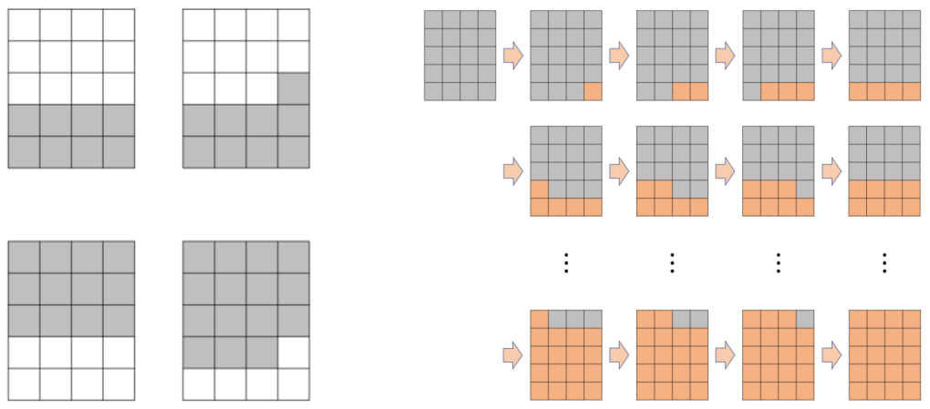
Figure 4.1. In the figures in this article, white, gray, and orange colors denote the spins $-1$, $0$, and $+1$, respectively. (Left) canonical configurations for $(K,\,L)=(4,\,5)$; $\zeta_{2}^{+}$, $\zeta_{2,1}^{+-}$ (upper-right), $\zeta_{3}^{-}$ (lower-left), and $\zeta_{3,3}^{-+}$. (Right) a canonical path from $\mathbf{0}$ to $\mathbf{+1}$ for $(K,\,L)=(4,\,5)$.

Definition 4.2 (Pre-canonical configurations and paths).

We define pre-canonical configurations between $\mathbf{-1}$ and $\mathbf{0}$. We refer to Figure 4.1 (left) for an illustration.

• For $v\in\llbracket 0,\,L\rrbracket$, we denote by $\zeta_{v}^{+}\in\mathcal{X}$ the spin configuration whose spins are $0$ on $\llbracket 1,\,K\rrbracket\times\llbracket 1,\,v\rrbracket$ and $-1$ on the remainder. Moreover, we denote by $\zeta_{v}^{-}\in\mathcal{X}$ the spin configuration whose spins are $0$ on $\llbracket 1,\,K\rrbracket\times\llbracket L-v+1,\,L\rrbracket$ and $-1$ on the remainder. Hence, we have $\zeta_{0}^{+}=\zeta_{0}^{-}=\mathbf{-1}$ and $\zeta_{L}^{+}=\zeta_{L}^{-}=\mathbf{0}$. For $v\in\llbracket 0,\,L\rrbracket$, we write

  $$\mathcal{R}_{v}=\{\zeta_{v}^{+},\,\zeta_{v}^{-}\}.$$ (4.1)

• For $v\in\llbracket 0,\,L-1\rrbracket$ and $h\in\llbracket 0,\,K\rrbracket$, we denote by $\zeta_{v,h}^{++}\in\mathcal{X}$ the configuration whose spins are $0$ on

  $$\big{[}\llbracket 1,\,K\rrbracket\times\llbracket 1,\,v\rrbracket\big{]}\cup\big{[}\llbracket 1,\,h\rrbracket\times\{v+1\}\big{]}$$

  and $-1$ on the remainder. Similarly, we denote by $\zeta_{v,h}^{+-}\in\mathcal{X}$ the configuration whose spins are $0$ on

  $$\big{[}\llbracket 1,\,K\rrbracket\times\llbracket 1,\,v\rrbracket\big{]}\cup\big{[}\llbracket K-h+1,\,K\rrbracket\times\{v+1\}\big{]}$$

  and $-1$ on the remainder. Namely, we obtain $\zeta_{v,h}^{++}$ (resp. $\zeta_{v,h}^{+-}$) from $\zeta_{v}^{+}$ by attaching a protuberance of spin $0$ of size $h$ at its upper-left (resp. upper-right) corner of the cluster of spin $0$. Similarly, we define $\zeta_{v,h}^{-+}$ and $\zeta_{v,h}^{--}$ by attaching a protuberance of spin $0$ of size $h$ in $\zeta_{v}^{-}$. For $v\in\llbracket 0,\,L-1\rrbracket$, we write

  $$\mathcal{Q}_{v}=\bigcup_{h=1}^{K-1}\{\zeta_{v,h}^{++},\,\zeta_{v,h}^{+-},\,\zeta_{v,h}^{-+},\,\zeta_{v,h}^{--}\}.$$ (4.2)

  Concisely, $\mathcal{Q}_{v}$ consists of the configurations which connect the ones in $\mathcal{R}_{v}$ and $\mathcal{R}_{v+1}$.

• We define the collection $\mathcal{C}$ of pre-canonical configurations as

  $$\mathcal{C}=\bigcup_{v=0}^{L}\mathcal{R}_{v}\cup\bigcup_{v=0}^{L-1}\mathcal{Q}_{v}.$$

• Finally, a sequence $(\omega_{n})_{n=0}^{KL}$ of configurations is a pre-canonical path if it satisfies the following conditions; see Figure 4.1 (right).

  • $\omega_{Kv}=\zeta_{v}^{+}$ for all $v\in\llbracket 0,\,L\rrbracket$ (Type 1) or $\omega_{Kv}=\zeta_{v}^{-}$ for all $v\in\llbracket 0,\,L\rrbracket$ (Type 2).

  • (Type 1) For each $v\in\llbracket 0,\,L-1\rrbracket$, $\omega_{Kv+h}=\zeta_{v,h}^{++}$ for all $h\in\llbracket 0,\,K\rrbracket$ or $\omega_{Kv+h}=\zeta_{v,h}^{+-}$ for all $h\in\llbracket 0,\,K\rrbracket$.

  • (Type 2) For each $v\in\llbracket 0,\,L-1\rrbracket$, $\omega_{Kv+h}=\zeta_{v,h}^{-+}$ for all $h\in\llbracket 0,\,K\rrbracket$ or $\omega_{Kv+h}=\zeta_{v,h}^{--}$ for all $h\in\llbracket 0,\,K\rrbracket$.

We can readily verify that a pre-canonical path is indeed a path, in the sense of Definition 2.2. Moreover, pre-canonical paths characterize all the possible paths from $\mathbf{-1}$ to $\mathbf{0}$ in $\mathcal{C}$ if $K<L$. However, more possible paths exist if $K=L$; that is, the transposed pre-canonical paths.

Based on this observation, we define canonical configurations and paths between the ground states as follows:

Definition 4.3 (Canonical configurations and paths).

For two spins $a$ and $b$, we denote by $\mathcal{X}^{a,b}\subseteq\mathcal{X}$ the collection of configurations of which all spins are either $a$ or $b$. Then, we define the natural one-to-one correspondence $\Xi^{a,b}:\mathcal{X}^{-1,0}\rightarrow\mathcal{X}^{a,b}$ which maps spins $-1$ and $0$ to $a$ and $b$, respectively.

Now, we fix a good pair $(a,\,b)$ (cf. Notation 4.1). Then, we divide into the cases of $K<L$ and $K=L$.

• (Case $K<L$) We define the collection $\mathcal{C}^{a,b}$ of canonical configurations between $\mathbf{a}$ and $\mathbf{b}$ as

  $$\mathcal{C}^{a,b}=\Xi^{a,b}(\mathcal{C}).$$

  By symmetry, using $\Xi^{b,a}$ instead of $\Xi^{a,b}$ yields the same result, so that $\mathcal{C}^{a,b}=\mathcal{C}^{b,a}$. Then, we define (cf. (4.1) and (4.2))

  $$\mathcal{R}_{v}^{a,b}=\Xi^{a,b}(\mathcal{R}_{v})\;\;\;\;;\;v\in\llbracket 0,\,L\rrbracket,\;\;\;\;\mathcal{Q}_{v}^{a,b}=\Xi^{a,b}(\mathcal{Q}_{v})\;\;\;\;;\;v\in\llbracket 0,\,L-1\rrbracket.$$

• (Case $K=L$) We define a transpose operator $\Theta:\mathcal{X}\rightarrow\mathcal{X}$ by, for $\sigma\in\mathcal{X}$,

  $$(\Theta(\sigma))(k,\,\ell)=\sigma(\ell,\,k)\;\;\;\;;\;k\in\llbracket 1,\,K\rrbracket\text{ and }\ell\in\llbracket 1,\,L\rrbracket.$$

  Then, we define the collection $\mathcal{C}^{a,b}$ of canonical configurations between $\mathbf{a}$ and $\mathbf{b}$ as

  $$\mathcal{C}^{a,b}=\Xi^{a,b}(\mathcal{C})\cup(\Theta\circ\Xi^{a,b})(\mathcal{C}).$$

  We enlarge the collection of canonical configurations in this case, because the transposed configurations also have the same energy due to the condition $K=L$. Again, we have $\mathcal{C}^{a,b}=\mathcal{C}^{b,a}$. Moreover, we define

  $$\mathcal{R}_{v}^{a,b} =\Xi^{a,b}(\mathcal{R}_{v})\cup(\Theta\circ\Xi^{a,b})(\mathcal{R}_{v})\;\;\;\;;\;v\in\llbracket 0,\,L\rrbracket,$$

  $$\mathcal{Q}_{v}^{a,b} =\Xi^{a,b}(\mathcal{Q}_{v})\cup(\Theta\circ\Xi^{a,b})(\mathcal{Q}_{v})\;\;\;\;;\;v\in\llbracket 0,\,L-1\rrbracket.$$

A sequence $(\omega_{n})_{n=0}^{KL}$ of configurations is a canonical path from $\mathbf{a}$ to $\mathbf{b}$ if there exists a pre-canonical path $(\widetilde{\omega}_{n})_{n=0}^{KL}$ such that $\omega_{n}=\Xi^{a,b}(\widetilde{\omega}_{n})$ for all $n\in\llbracket 0,\,KL\rrbracket$ (or additionally $\omega_{n}=(\Theta\circ\Xi^{a,b})(\widetilde{\omega}_{n})$ for all $n\in\llbracket 0,\,KL\rrbracket$ if $K=L$).

Remark 4.4.

It holds that $H(\sigma)\leq\Gamma$ for all $\sigma\in\mathcal{C}^{-1,0}\cup\mathcal{C}^{0,+1}$ and

$$H(\sigma)=\begin{cases}\Gamma-1&\text{if }\sigma\in\mathcal{R}_{v}^{-1,0}\cup\mathcal{R}_{v}^{0,+1}\text{ for }v\in\llbracket 1,\,L-1\rrbracket,\\ \Gamma&\text{if }\sigma\in\mathcal{Q}_{v}^{-1,0}\cup\mathcal{Q}_{v}^{0,+1}\text{ for }v\in\llbracket 1,\,L-2\rrbracket.\end{cases}$$

These facts imply that canonical paths are $\Gamma$-paths.

Remark 4.5.

One may be tempted to define similar objects between $\mathbf{-1}$ and $\mathbf{+1}$ by choosing $(a,\,b)=(-1,\,+1)$ or $(+1,\,-1)$. However, the resulting configurations have too high energy to be considered in our investigation. To explain this, recall $\Xi^{-1,+1}:\mathcal{X}^{-1,0}\rightarrow\mathcal{X}^{-1,+1}$ from Definition 4.3. Then, we can deduce that

$$H(\sigma)=\begin{cases}4\Gamma-4&\text{if }\sigma\in\Xi^{-1,+1}(\mathcal{R}_{v})\text{ for }v\in\llbracket 1,\,L-1\rrbracket,\\ 4\Gamma&\text{if }\sigma\in\Xi^{-1,+1}(\mathcal{Q}_{v})\text{ for }v\in\llbracket 1,\,L-2\rrbracket,\end{cases}$$

where $4\Gamma-4>\Gamma$. Hence, we cannot connect $\mathbf{-1}$ and $\mathbf{+1}$ by a direct canonical $\Gamma$-path, and thus it is natural to expect that $\Gamma$-paths between $\mathbf{-1}$ and $\mathbf{+1}$ must visit at least a certain neighborhood of $\mathbf{0}$. Rigorously, this is exactly part (1) of Theorem 2.7.

4.2. Proof of Theorem 2.3

Based on the canonical configurations, we are now ready to prove that the energy barrier of the dynamics is exactly $\Gamma$.

Proof of Theorem 2.3.

First, we claim that for two spins $a$ and $b$,

$$\Gamma_{a,b}=\Phi(\mathbf{a},\,\mathbf{b})\leq\Gamma.$$ (4.3)

Indeed, the canonical paths between $\mathbf{-1}$ and $\mathbf{0}$ assert that $\Gamma_{-1,0}=\Phi(\mathbf{-1},\,\mathbf{0})\leq\Gamma$. Similarly, the canonical paths between $\mathbf{0}$ and $\mathbf{+1}$ imply $\Gamma_{0,+1}\leq\Gamma$. Hence,

$$\Gamma_{-1,+1}=\Phi(\mathbf{-1},\,\mathbf{+1})\leq\max\{\Phi(\mathbf{-1},\,\mathbf{0}),\,\Phi(\mathbf{0},\,\mathbf{+1})\}\leq\Gamma.$$

Thus, we get (4.3). Therefore, to conclude the proof of Theorem 2.3, it suffices to prove that for distinct spins $a$ and $b$,

$$\Gamma_{a,b}=\Phi(\mathbf{a},\,\mathbf{b})\geq\Gamma.$$ (4.4)

To provide a simple proof of (4.4), we recall the Metropolis dynamics of the 2D Potts model for $q=3$ with zero external field [14, 21]. In this model, everything is defined in the same way as in Section 2.1, except that the Hamiltonian is given by

$$H_{\mathrm{Potts}}(\sigma)=\sum_{x\sim y}\mathbf{1}\{\sigma(x)\neq\sigma(y)\}\;\;\;\;;\;\sigma\in\mathcal{X}.$$ (4.5)

Comparing this to our Hamiltonian (2.3), we can easily notice that

$$H(\sigma)\geq H_{\mathrm{Potts}}(\sigma)\;\;\;\;;\;\sigma\in\mathcal{X}.$$ (4.6)

Moreover, it is proved in [21, Theorem 2.1] that the energy barrier $\Phi_{\mathrm{Potts}}(\mathbf{s},\,\mathbf{s}^{\prime})$, $\mathbf{s},\,\mathbf{s}^{\prime}\in\mathcal{S}$, of the Potts dynamics is exactly $\Gamma$. Therefore, as the energy landscapes of the two models are identical, we deduce from (4.6) that

$$\Phi(\mathbf{s},\,\mathbf{s}^{\prime})\geq\Phi_{\mathrm{Potts}}(\mathbf{s},\,\mathbf{s}^{\prime})=\Gamma\;\;\;\;;\;\mathbf{s},\,\mathbf{s}^{\prime}\in\mathcal{S}.$$

This is exactly (4.4), and thus we conclude the proof of Theorem 2.3. ∎

4.3. Neighborhoods and configurations with small energy

First, we review the concept of neighborhoods defined in [14, Section 5].

Definition 4.6 (Neighborhoods).

We define two types of neighborhoods of configurations as in [14, Definition 5.1].

1. For $\sigma\in\mathcal{X}$, the neighborhoods $\mathcal{N}(\sigma)$ and $\widehat{\mathcal{N}}(\sigma)$ are defined as (cf. Definition 2.2)

   $$\mathcal{N}(\sigma) =\{\zeta\in\mathcal{X}:\exists\text{a }(\Gamma-1)\text{-path }(\omega_{n})_{n=0}^{N}\text{ connecting }\sigma\text{ and }\zeta\},$$

   $$\widehat{\mathcal{N}}(\sigma) =\{\zeta\in\mathcal{X}:\exists\text{a }\Gamma\text{-path }(\omega_{n})_{n=0}^{N}\text{ connecting }\sigma\text{ and }\zeta\}.$$

   Then, for $\mathcal{A}\subseteq\mathcal{X}$, we define

   $$\mathcal{N}(\mathcal{A})=\bigcup_{\sigma\in\mathcal{A}}\mathcal{N}(\sigma)\;\;\;\;\text{and\;\;\;\;}\widehat{\mathcal{N}}(\mathcal{A})=\bigcup_{\sigma\in\mathcal{A}}\mathcal{\widehat{\mathcal{N}}}(\sigma).$$

2. Let $\mathcal{B}\subseteq\mathcal{X}$. For $\sigma\in\mathcal{X}$ with $\sigma\notin\mathcal{B}$, we define

   $$\widehat{\mathcal{N}}(\sigma;\mathcal{B})=\{\zeta\in\mathcal{X}:\exists\text{a }\Gamma\text{-path in }\mathcal{X}\setminus\mathcal{B}\text{ connecting }\sigma\text{ and }\zeta\}.$$

   Then, for $\mathcal{A}\subseteq\mathcal{X}$ disjoint with $\mathcal{B}$, we define

   $$\widehat{\mathcal{N}}(\mathcal{A};\mathcal{B})=\bigcup_{\sigma\in\mathcal{A}}\widehat{\mathcal{N}}(\sigma;\mathcal{B}).$$

With these notions in mind, as $\beta\rightarrow\infty$, the only configurations relevant to the study of metastability are those in $\widehat{\mathcal{N}}(\mathcal{S})$ (in view of Theorem 2.3). Indeed, if we take $\sigma\in\mathcal{X}$ with $H(\sigma)>\Gamma$, then by (2.9) it holds that, for any $\zeta\in\mathcal{X}$ with $\zeta\sim\sigma$,

$$\mu_{\beta}(\sigma)c_{\beta}(\sigma,\,\zeta)=\mu_{\beta}(\zeta)c_{\beta}(\zeta,\,\sigma)\leq\mu_{\beta}(\sigma)=O(e^{-\beta(\Gamma+1)}).$$

This implies that any spin updates associated with $\sigma$ are irrelevant to the study of metastability on the scale $e^{\beta\Gamma}$. Hence, $\widehat{\mathcal{N}}(\mathcal{S})$ is the main object in our study of the energy landscape.

The following lemma, which is a generalization of [14, Lemma 5.2], is useful to investigate the $\widehat{\mathcal{N}}$-neighborhoods. We can prove this lemma in the same manner, and thus we omit it.

Lemma 4.7.

Suppose that $\mathcal{A}$, $\mathcal{A}^{\prime}$, and $\mathcal{B}$ are pairwise disjoint subsets of $\mathcal{X}$. Then, we have

$$\widehat{\mathcal{N}}(\mathcal{A}\cup\mathcal{A}^{\prime};\mathcal{B})=\widehat{\mathcal{N}}(\mathcal{A}^{\prime};\mathcal{A}\cup\mathcal{B})\cup\widehat{\mathcal{N}}(\mathcal{A};\mathcal{A}^{\prime}\cup\mathcal{B}).$$

In particular, if $\mathcal{B}=\emptyset$, then we have $\widehat{\mathcal{N}}(\mathcal{A}\cup\mathcal{A}^{\prime})=\widehat{\mathcal{N}}(\mathcal{A}^{\prime};\mathcal{A})\cup\widehat{\mathcal{N}}(\mathcal{A};\mathcal{A}^{\prime})$.

We verified in Section 4.2 that the energy barrier is exactly $\Gamma$. Now, we fully characterize the spin configurations with energy less than $\Gamma$. This result is an analogue of [14, Proposition 6.8] and can be proved in a similar manner; thus, we omit the proof. We refer to Figure 4.2 for some examples of such configurations.

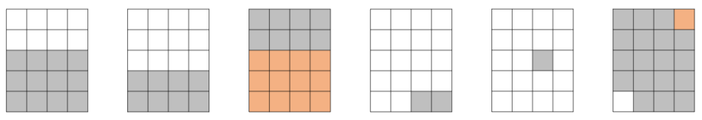
Figure 4.2. Configurations with energy smaller than $\Gamma$: type (T1) (the first three) and type (T2) (the last three).

Proposition 4.8.

Suppose that $\sigma\in\mathcal{X}$ satisfies $H(\sigma)<\Gamma$. Then, exactly one of (T1) or (T2) below holds.

1. There exist a good pair $(a,\,b)$ and $v\in\llbracket 2,\,L-2\rrbracket$ such that $\sigma\in\mathcal{R}_{v}^{a,b}$. In particular, $\mathcal{N}(\sigma)$ is a singleton, i.e., $\mathcal{N}(\sigma)=\{\sigma\}$.

2. The configuration $\sigma$ belongs to $\mathcal{N}(\mathbf{a})$ for exactly one spin $a$, so that $\mathcal{N}(\sigma)=\mathcal{N}(\mathbf{a})$.

4.4. Proof of Theorem 2.4

In this subsection, we prove Theorem 2.4. To this end, we need the following result regarding the valley depths of the entire energy landscape.

Lemma 4.9.

We have the following upper bounds for the depths of the valleys:

1. For all $\sigma\in\mathcal{X}$ and $\mathbf{s}\in\mathcal{S}$, it holds that $\Phi(\sigma,\,\mathbf{s})-H(\sigma)\leq\Gamma$.

2. For all $\sigma\in\mathcal{X}\setminus\mathcal{S}$, it holds that $\Phi(\sigma,\,\mathcal{S})-H(\sigma)<\Gamma$.

Proof.

The same assertions for the Metropolis dynamics on the Potts model are proved in [21, Theorem 2.1]. Because the same arguments work for our Blume–Capel model as well, we omit the proof. ∎

Remark 4.10.

An alternative proof can be found in [14, Lemma 6.11] which provides an explicit path that guarantees the upper bounds stated in Lemma 4.9.

Based on the previous lemma, we give a formal proof of Theorem 2.4.

Proof of Theorem 2.4.

By the general theory developed in [21, 22], Theorem 2.3 and Lemma 4.9 are sufficient to conclude the assertions on the transition time, mixing time, and spectral gap given in Theorem 2.4. ∎

5. Typical and Gateway Configurations

In this section, we define the concepts of typical and gateway configurations and investigate their several basic properties. The concepts are analogues of those defined in [14, Section 7]. We note that even though the results are similar to those in [14], we still thoroughly review the notation here because there indeed exist technical differences due to the non-symmetry of the Blume–Capel model (cf. Remark 2.1).

5.1. Typical configurations

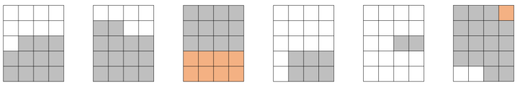
Figure 5.1. Typical configurations: bulk ones (the first three) and edge ones (the last three).

Definition 5.1 (Typical configurations).

Here, we define typical configurations. We refer to Figure 5.1 for a visualization.

• Fix a good pair $(a,\,b)$. The collection of bulk typical configurations between $\mathbf{a}$ and $\mathbf{b}$ is defined as

  $$\mathcal{B}^{a,b}=\bigcup_{v=2}^{L-2}\mathcal{R}_{v}^{a,b}\cup\bigcup_{v=2}^{L-3}\mathcal{Q}_{v}^{a,b}.$$ (5.1)

  Moreover, we define (cf. Remark 4.4)

  $$\mathcal{B}_{\Gamma}^{a,b}=\bigcup_{v=2}^{L-3}\mathcal{Q}_{v}^{a,b}=\{\sigma\in\mathcal{B}^{a,b}:H(\sigma)=\Gamma\}.$$

  Clearly, we have $\mathcal{B}^{a,b}=\mathcal{B}^{b,a}$ and $\mathcal{B}_{\Gamma}^{a,b}=\mathcal{B}_{\Gamma}^{b,a}$.

• For a spin $a$, the collection of edge typical configurations near $\mathbf{a}$ is defined as

  $$\mathcal{E}^{a}=\widehat{\mathcal{N}}(\mathbf{a};\mathcal{B}_{\Gamma}^{-1,0}\cup\mathcal{B}_{\Gamma}^{0,+1}).$$ (5.2)

• Finally, the collection of typical configurations is defined as

  $$\mathcal{T}=\mathcal{B}^{-1,0}\cup\mathcal{B}^{0,+1}\cup\mathcal{E}^{-1}\cup\mathcal{E}^{0}\cup\mathcal{E}^{+1}.$$ (5.3)

Then, we summarize the following properties for the typical configurations. Rigorous verifications can be found in [14, Section 7.2] and thus we do not repeat them.

Proposition 5.2.

The following properties hold for the typical configurations.

1. The collections $\mathcal{E}^{-1}$, $\mathcal{E}^{0}$, and $\mathcal{E}^{+1}$ are disjoint.

2. We have

   $$\mathcal{E}^{-1}\cap\mathcal{B}^{-1,0} =\mathcal{R}_{2}^{-1,0},\;\;\;\;\mathcal{E}^{0}\cap\mathcal{B}^{-1,0}=\mathcal{R}_{L-2}^{-1,0},$$ (5.4)

   $$\mathcal{E}^{+1}\cap\mathcal{B}^{0,+1} =\mathcal{R}_{L-2}^{0,+1},\;\;\;\;\mathcal{E}^{0}\cap\mathcal{B}^{0,+1}=\mathcal{R}_{2}^{0,+1}.$$ (5.5)

3. We have $\mathcal{E}^{-1}\cap\mathcal{B}^{0,+1}=\mathcal{E}^{+1}\cap\mathcal{B}^{-1,0}=\emptyset$.

4. Recall the definition (5.3) of $\mathcal{T}$. Then, $\widehat{\mathcal{N}}(\mathcal{S})=\mathcal{T}$.

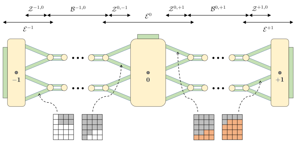
Figure 5.2. Energy landscape of $\widehat{\mathcal{N}}(\mathcal{S})$ for the case of $K<L$. Green regions represent the configurations with energy exactly $\Gamma$, and yellow regions represent the ones with energy less than $\Gamma$. Configurations below are examples of gateway configurations.

Remark 5.3 (Edge structure of typical configurations).

Based on Proposition 5.2, we have the following decomposition of $E(\widehat{\mathcal{N}}(\mathcal{S}))=E(\mathcal{T})$ (see Figure 5.2 for the full energy landscape):

$$E(\widehat{\mathcal{N}}(\mathcal{S}))=E(\mathcal{B}^{-1,0})\cup E(\mathcal{B}^{0,+1})\cup E(\mathcal{E}^{-1})\cup E(\mathcal{E}^{0})\cup E(\mathcal{E}^{+1}).$$

To prove this fact, we check that the members constituting $\mathcal{T}$ (cf. (5.3)) are separated, in the sense that for members $\mathcal{A}$ and $\mathcal{A}^{\prime}$,

$$\{\sigma,\,\sigma^{\prime}\}\in E(\mathcal{A}\cup\mathcal{A}^{\prime})\;\;\;\;\text{implies}\;\;\;\;\sigma,\,\sigma^{\prime}\in\mathcal{A}\text{ or }\sigma,\,\sigma^{\prime}\in\mathcal{A}^{\prime}.$$

Indeed, $\mathcal{E}^{a}$ for spins $a$ are separated by part (1) of Proposition 5.2. The collections $\mathcal{B}^{-1,0}$ and $\mathcal{B}^{0,+1}$ are clearly separated.

To check that a bulk collection $\mathcal{B}^{a,b}$ and an edge collection $\mathcal{E}^{a^{\prime}}$ are separated, it suffices to prove that if $\sigma\in\mathcal{B}^{a,b}$ and $\sigma^{\prime}\in\mathcal{E}^{a^{\prime}}\setminus\mathcal{B}^{a,b}$ with $\sigma\sim\sigma^{\prime}$, then $\sigma\in\mathcal{E}^{a^{\prime}}$. To this end, as $\sigma^{\prime}\notin\mathcal{B}^{a,b}$, we must have $\sigma\in\mathcal{R}_{2}^{a,b}$ or $\sigma\in\mathcal{R}_{L-2}^{a,b}$. For the former case, as $\mathcal{R}_{2}^{a,b}\subseteq\mathcal{E}^{a}$, by part (1) of Proposition 5.2 we obtain $a=a^{\prime}$ and thus $\sigma\in\mathcal{E}^{a^{\prime}}$. For the latter case, as $\mathcal{R}_{L-2}^{a,b}\subseteq\mathcal{E}^{b}$, we obtain $b=a^{\prime}$ and thus $\sigma\in\mathcal{E}^{a^{\prime}}$.

5.2. Gateway configurations

Here, we define gateway configurations of the dynamics. We again refer to Figure 5.2 for a visualization of the role and examples of gateway configurations.

Definition 5.4 (Gateway configurations).

As for the typical configurations, we define gateway configurations between $\mathbf{a}$ and $\mathbf{b}$ for good pairs $(a,\,b)$. Thus, we fix a good pair $(a,\,b)$. We define $\mathcal{Z}^{a,b}$ as

$$\{\sigma\in\mathcal{X}: \exists\text{a path }(\omega_{n})_{n=0}^{N}\text{ in }\mathcal{X}\setminus\mathcal{B}_{\Gamma}^{a,b}\text{ with }N\geq 1\text{ such that}$$

$$\omega_{0}\in\mathcal{R}_{2}^{a,b},\;\omega_{N}=\sigma,\;\text{and}\;H(\omega_{n})=\Gamma\text{ for all }n\in\llbracket 1,\,N\rrbracket\}.$$ (5.6)

Note that $\mathcal{Z}^{a,b}\neq\mathcal{Z}^{b,a}$. Then, we define the collection of gateway configurations between $\mathbf{a}$ and $\mathbf{b}$ as

$$\mathcal{G}^{a,b}=\mathcal{Z}^{a,b}\cup\mathcal{B}^{a,b}\cup\mathcal{Z}^{b,a},$$ (5.7)

which is indeed a decomposition of $\mathcal{G}^{a,b}$. As $\mathcal{B}^{a,b}=\mathcal{B}^{b,a}$, we have $\mathcal{G}^{a,b}=\mathcal{G}^{b,a}$.

Then, we have the following properties for the gateway configurations.

Lemma 5.5.

Fix a good pair $(a,\,b)$ and suppose that $\sigma,\,\zeta\in\mathcal{X}$ satisfy

$$\sigma\in\mathcal{G}^{a,b},\;\zeta\notin\mathcal{G}^{a,b},\;\sigma\sim\zeta,\;\text{and}\;H(\zeta)\leq\Gamma.$$

Then, we have either $\zeta\in\mathcal{N}(\mathbf{a})$ and $\sigma\in\mathcal{Z}^{a,b}$ or $\zeta\in\mathcal{N}(\mathbf{b})$ and $\sigma\in\mathcal{Z}^{b,a}$.

Proof.

This lemma can be proved in an identical manner to [14, Lemma 8.5]. ∎

5.3. Lemma on equilibrium potentials and proof of Theorem 2.7

In this subsection, we prove Theorem 2.7. Before providing the proof, we give an elementary estimate on equilibrium potentials (cf. (3.2)), which is a generalization of [14, Lemma 10.4]. This lemma is used in the proof of Theorem 2.7 and later in Section 8 to estimate the test flow. We refer to [14, Lemmas 10.4 and 16.5] for the proof.

Lemma 5.6.

For disjoint and non-empty subsets $\mathcal{A}$ and $\mathcal{B}$ of $\mathcal{S}$, there exists $C=C(K,\,L)>0$ such that for all $\mathbf{s}\in\mathcal{S}$,

$$\max_{\zeta\in\mathcal{N}(\mathbf{s})}\big{|}\mathbb{P}_{\zeta}^{\beta}[\tau_{\mathcal{A}}<\tau_{\mathcal{B}}]-\mathbb{P}_{\mathbf{s}}^{\beta}[\tau_{\mathcal{A}}<\tau_{\mathcal{B}}]\big{|}\leq Ce^{-\beta}.$$ (5.8)

Then, we provide a proof of Theorem 2.7.

Proof of Theorem 2.7.

Part (2) is obvious from the model symmetry. Thus, to conclude the proof, we prove part (1). We first prove that

$$\lim_{\beta\rightarrow\infty}\mathbb{P}_{\mathbf{-1}}^{\beta}[\tau_{\mathcal{N}(\mathbf{0})}<\tau_{\mathbf{+1}}]=1.$$ (5.9)

We denote by $\tau^{*}$ the hitting time of the set $\{\sigma\in\mathcal{X}:H(\sigma)\geq\Gamma+1\}$. Then, [22, Theorem 3.2] implies that

$$\mathbb{P}_{\mathbf{-1}}^{\beta}[\tau^{*}>e^{\beta(\Gamma+1/2)}]=1-o(1).$$

Hence, by part (1) of Theorem 2.4 with $\epsilon=1/2$, we have

$$\mathbb{P}_{\mathbf{-1}}^{\beta}[\tau_{\mathbf{+1}}<\tau^{*}]=1-\mathbb{P}_{\mathbf{-1}}^{\beta}[\tau_{\mathbf{+1}}\geq\tau^{*}] =1-o(1)-\mathbb{P}_{\mathbf{-1}}^{\beta}[\tau_{\mathbf{+1}}\geq\tau^{*}>e^{\beta(\Gamma+1/2)}]$$

$$\geq 1-o(1)-\mathbb{P}_{\mathbf{-1}}^{\beta}[\tau_{\mathbf{+1}}>e^{\beta(\Gamma+1/2)}]=1-o(1).$$

Therefore, it suffices to prove that a $\Gamma$-path from $\mathbf{-1}$ to $\mathbf{+1}$ must visit $\mathcal{N}(\mathbf{0})$. To this end, we fix a $\Gamma$-path $(\omega_{n})_{n=0}^{N}$ with $\omega_{0}=\mathbf{-1}\in\mathcal{E}^{-1}$ and $\omega_{N}=\mathbf{+1}\in\mathcal{E}^{+1}$. Then, by Proposition 5.2 and Remark 5.3, starting from $\mathbf{-1}\in\mathcal{E}^{-1}$, this path must successively visit $\mathcal{E}^{-1}\cap\mathcal{B}^{-1,0}=\mathcal{R}_{2}^{-1,0}$, $\mathcal{B}^{-1,0}$, $\mathcal{B}^{-1,0}\cap\mathcal{E}^{0}=\mathcal{R}_{2}^{0,-1}$, $\mathcal{E}^{0}$, $\mathcal{E}^{0}\cap\mathcal{B}^{0,+1}=\mathcal{R}_{2}^{0,+1}$, $\mathcal{B}^{0,+1}$, and $\mathcal{B}^{0,+1}\cap\mathcal{E}^{+1}=\mathcal{R}_{2}^{+1,0}$ to finally arrive at $\mathbf{+1}\in\mathcal{E}^{+1}$. Thus, the following time is well defined:

$$n_{0}=\max\{n:\omega_{n}\in\mathcal{R}_{2}^{0,-1}\}.$$

Then, by the definition of gateway configurations, we have $\omega_{n_{0}+1}\in\mathcal{Z}^{0,-1}$. Then, by defining

$$n_{1}=\min\{n>n_{0}:\omega_{n}\notin\mathcal{G}^{0,-1}\},$$

we have $\omega_{n_{1}}\in\mathcal{N}(\mathbf{0})$ by Lemma 5.5, which concludes the proof of (5.9).

Moreover, Lemma 5.6 with $\mathcal{A}=\{\mathbf{0}\}$, $\mathcal{B}=\{\mathbf{+1}\}$, and $\mathbf{s}=\mathbf{0}$ implies that

$$\max_{\sigma\in\mathcal{N}(\mathbf{0})}\mathbb{P}_{\sigma}^{\beta}[\tau_{\mathbf{0}}<\tau_{\mathbf{+1}}]=1-o(1).$$

This is equivalent to

$$\lim_{\beta\rightarrow\infty}\max_{\sigma\in\mathcal{N}(\mathbf{0})}\mathbb{P}_{\sigma}^{\beta}[\tau_{\mathbf{0}}<\tau_{\mathbf{+1}}]=1.$$ (5.10)

Therefore, we conclude the proof of the first assertion of part (1) with (5.9) and (5.10) by the casual argument using the strong Markov property. The second assertion follows identically. ∎

6. Edge Typical Configurations

In this section, we focus on the edge typical configurations defined in Definition 5.1, which have much more complex geometry than the bulk typical configurations. This section is an analogue of [14, Section 7.3], but we provide here a much more detailed and quantitative analysis on the behavior of the edge typical configurations.

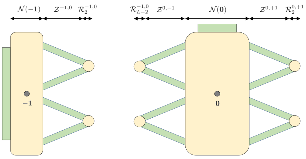
Figure 6.1. Edge typical configurations when $K<L$. (Left) structure of $\mathcal{E}^{-1}$. (Right) structure of $\mathcal{E}^{0}$.

6.1. Projected graph

We consistently refer to Figure 6.1 for an illustration of the notions defined in this subsection. For each spin $a$, we decompose $\mathcal{E}^{a}=\mathcal{I}^{a}\cup\mathcal{O}^{a}$ where

$$\mathcal{O}^{a}=\{\sigma\in\mathcal{E}^{a}:H(\sigma)=\Gamma\}\;\;\;\;\text{and}\;\;\;\;\mathcal{I}^{a}=\{\sigma\in\mathcal{E}^{a}:H(\sigma)<\Gamma\}.$$

By Proposition 4.8, we notice that

$$\mathcal{I}^{a}=\mathcal{N}(\mathbf{a})\cup\Big{[}\bigcup_{b:\,(a,b)\text{ is good}}\mathcal{R}_{2}^{a,b}\Big{]}.$$ (6.1)

We further define

$$\mathcal{I}_{\mathfrak{0}}^{a}=\{\mathbf{a}\}\cup\Big{[}\bigcup_{b:\,(a,b)\text{ is good}}\mathcal{R}_{2}^{a,b}\Big{]},$$ (6.2)

so that each $\sigma\in\mathcal{I}^{a}$ satisfies $\sigma\in\mathcal{N}(\zeta)$ for exactly one $\zeta\in\mathcal{I}_{\mathfrak{0}}^{a}$. Hence, we get the following alternative decomposition of $\mathcal{E}^{a}$:

$$\mathcal{E}^{a}=\mathcal{O}^{a}\cup\Big{[}\bigcup_{\zeta\in\mathcal{I}_{\mathfrak{0}}^{a}}\mathcal{N}(\zeta)\Big{]}.$$ (6.3)

We chose the set of representatives $\mathcal{I}_{\mathfrak{0}}^{a}$ because configurations belonging to the same $\mathcal{N}$-neighborhood are not distinguished in the study of metastability, in the sense of Lemma 5.6.

Remark 6.1.

We remark on the display (6.1). In details, we have

$$\mathcal{I}^{-1}=\mathcal{N}(\mathbf{-1})\cup\mathcal{R}_{2}^{-1,0}\;\;\;\;\text{and}\;\;\;\;\mathcal{I}^{+1}=\mathcal{N}(\mathbf{+1})\cup\mathcal{R}_{L-2}^{0,+1},$$

whereas

$$\mathcal{I}^{0}=\mathcal{N}(\mathbf{0})\cup\mathcal{R}_{L-2}^{-1,0}\cup\mathcal{R}_{2}^{0,+1}.$$

Hence, the structures of $\mathcal{E}^{-1}$ and $\mathcal{E}^{+1}$ are exactly the same, but they differ from the structure of $\mathcal{E}^{0}$. Figure 6.1 illustrates this difference.

Now, we define a graph structure on $\mathcal{O}^{a}\cup\mathcal{I}_{\mathfrak{0}}^{a}$.

Definition 6.2.

We fix spin $a$ and introduce a graph structure and a Markov chain on $\mathcal{O}^{a}\cup\mathcal{I}_{\mathfrak{0}}^{a}$.

• (Graph) Vertex set $\mathscr{V}^{a}$ is defined by

  $$\mathscr{V}^{a}=\mathcal{O}^{a}\cup\mathcal{I}_{\mathfrak{0}}^{a}.$$ (6.4)

  Then, the edge set $E(\mathscr{V}^{a})$ is defined as follows: $\{\sigma,\,\sigma^{\prime}\}\in E(\mathscr{V}^{a})$ if and only if either $\sigma,\,\sigma^{\prime}\in\mathcal{O}^{a}$ and $\sigma\sim\sigma^{\prime}$, or $\sigma\in\mathcal{O}^{a}$, $\sigma^{\prime}\in\mathcal{I}_{\mathfrak{0}}^{a}$, and $\sigma\sim\zeta$ for some $\zeta\in\mathcal{N}(\sigma^{\prime})$.

• (Markov chain) We define a transition rate $r^{\mathbf{a}}:\mathscr{V}^{a}\times\mathscr{V}^{a}\rightarrow[0,\,\infty)$ as follows: If $\{\sigma,\,\sigma^{\prime}\}\notin E(\mathscr{V}^{a})$, then $r^{\mathbf{a}}(\sigma,\,\sigma^{\prime})=0$. If $\{\sigma,\,\sigma^{\prime}\}\in E(\mathscr{V}^{a})$, then

  $$r^{\mathbf{a}}(\sigma,\,\sigma^{\prime})=\begin{cases}1&\text{if }\sigma,\,\sigma^{\prime}\in\mathcal{O}^{a},\\ |\{\zeta\in\mathcal{N}(\sigma):\zeta\sim\sigma^{\prime}\}|&\text{if }\sigma\in\mathcal{I}_{\mathfrak{0}}^{a},\;\sigma^{\prime}\in\mathcal{O}^{a},\\ |\{\zeta\in\mathcal{N}(\sigma^{\prime}):\zeta\sim\sigma\}|&\text{if }\sigma\in\mathcal{O}^{a},\;\sigma^{\prime}\in\mathcal{I}_{\mathfrak{0}}^{a}.\end{cases}$$ (6.5)

  Then, we define $\{Z^{a}(t)\}_{t\geq 0}$ as the continuous-time Markov chain on $\mathscr{V}^{a}$ with transition rate $r^{\mathbf{a}}(\cdot,\,\cdot)$. As the rate is symmetric, the Markov chain $Z^{a}(\cdot)$ is reversible with respect to its invariant distribution, which is the uniform distribution on $\mathscr{V}^{a}$.

Next, we prove that the process $Z^{a}(\cdot)$ approximates the Metropolis dynamics on the edge typical configurations.

Proposition 6.3.

For each spin $a$, define a projection map $\Pi^{\mathbf{a}}:\mathcal{E}^{a}\rightarrow\mathscr{V}^{a}$ by

$$\Pi^{\mathbf{a}}(\sigma)=\begin{cases}\sigma&\text{if }\sigma\in\mathcal{O}^{a},\\ \zeta&\text{if }\sigma\in\mathcal{N}(\zeta)\text{ for some }\zeta\in\mathcal{I}_{\mathfrak{0}}^{a}.\end{cases}$$

Then, there exists a constant $C=C(K,\,L)>0$ such that

1. for $\sigma_{1},\,\sigma_{2}\in\mathcal{O}^{a}$, we have

   $$\Big{|}\frac{1}{3}e^{-\beta\Gamma}r^{\mathbf{a}}(\Pi^{\mathbf{a}}(\sigma_{1}),\,\Pi^{\mathbf{a}}(\sigma_{2}))-\mu_{\beta}(\sigma_{1})c_{\beta}(\sigma_{1},\,\sigma_{2})\Big{|}\leq Ce^{-\beta(\Gamma+1)},$$

2. for $\sigma_{1}\in\mathcal{O}^{a}$ and $\sigma_{2}\in\mathcal{I}_{\mathfrak{0}}^{a}$, we have

   $$\Big{|}\frac{1}{3}e^{-\beta\Gamma}r^{\mathbf{a}}(\Pi^{\mathbf{a}}(\sigma_{1}),\,\Pi^{\mathbf{a}}(\sigma_{2}))-\sum_{\zeta\in\mathcal{N}(\sigma_{2})}\mu_{\beta}(\sigma_{1})c_{\beta}(\sigma_{1},\,\zeta)\Big{|}\leq Ce^{-\beta(\Gamma+1)}.$$

Proof.

As the proof is identical to that of [14, Proposition 7.7], we omit the details. ∎

6.2. Approximation to auxiliary process

In this subsection, we prove that the auxiliary process analyzed in Section A.1 successfully represents the Markov chain $Z^{a}(\cdot)$. First, we handle the case of $K<L$.

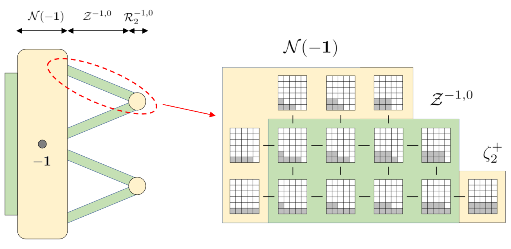
Figure 6.2. Visualization of Lemma 6.4 for $(K,\,L)=(5,\,6)$.

Lemma 6.4.

Suppose that $K<L$. Fix a good pair $(a,\,b)$ and recall the projected auxiliary process in Section A.2. Then, there exists a surjective mapping $\Phi^{a,b}:\mathscr{V}^{a}\rightarrow V_{K}$ which satisfies:

1. for each $\{\sigma,\,\sigma^{\prime}\}\in E(\mathscr{V}^{a})$ with $\{\sigma,\,\sigma^{\prime}\}\cap\mathcal{Z}^{a,b}=\emptyset$, we have $\Phi^{a,b}(\sigma)=\Phi^{a,b}(\sigma^{\prime})$,

2. for each $\{\sigma,\,\sigma^{\prime}\}\in E(\mathscr{V}^{a})$ with $\{\sigma,\,\sigma^{\prime}\}\cap\mathcal{Z}^{a,b}\neq\emptyset$, we have $\{\Phi^{a,b}(\sigma),\,\Phi^{a,b}(\sigma^{\prime})\}\in E(V_{K})$ and $r^{\mathbf{a}}(\sigma,\,\sigma^{\prime})=r_{K}(\Phi^{a,b}(\sigma),\,\Phi^{a,b}(\sigma^{\prime}))$,

3. for each $\{x,\,y\}\in E(V_{K})$, there exist exactly four edges $\{\sigma,\,\sigma^{\prime}\}\in E(\mathscr{V}^{a})$ such that $\{\Phi^{a,b}(\sigma),\,\Phi^{a,b}(\sigma^{\prime})\}=\{x,\,y\}$.

Proof.

First, we assume that $(a,\,b)=(-1,\,0)$. We refer to Figure 6.2 to provide insight of the proof given here. We have $\mathcal{R}_{2}^{-1,0}=\{\zeta_{2}^{+},\,\zeta_{2}^{-}\}$ (cf. Definition 4.3). First, we focus on the landscape between $\mathcal{N}(\mathbf{-1})$ and $\zeta_{2}^{+}$.

There are two possible $\sigma\in\mathcal{Z}^{-1,0}$ with $\sigma\sim\zeta_{2}^{+}$; that is, $\zeta_{1,K-1}^{++}$ and $\zeta_{1,K-1}^{+-}$. we first consider $\zeta_{1,K-1}^{++}$. All the possible paths from $\zeta_{1,K-1}^{++}$ to $\mathcal{N}(\mathbf{-1})$ are illustrated in Figure 6.2 (right) for the case of $K=5$ and $L=6$. Rigorously, we temporarily denote by $\xi_{h}\in\mathcal{X}$, $h\in\llbracket 1,\,K-1\rrbracket$ the configuration which has spins $0$ on

$$\big{[}\llbracket 1,\,K-1\rrbracket\times\{1\}\big{]}\cup\big{[}\llbracket 1,\,h\rrbracket\times\{2\}\big{]}$$

and spins $-1$ on the remainder. Then, we define $\Phi_{1}^{-1,0}:\{\mathbf{-1}\}\cup\bigcup_{h=1}^{K-1}\{\zeta_{1,h}^{++},\,\xi_{h}\}\cup\{\zeta_{2}^{+}\}\rightarrow V_{K}$ by $\Phi_{1}^{-1,0}(\zeta_{2}^{+})=0$, $\Phi_{1}^{-1,0}(\mathbf{-1})=\mathfrak{d}$, and for $h\in\llbracket 1,\,K-1\rrbracket$,

$$\Phi_{1}^{-1,0}(\zeta_{1,h}^{++})=(0,\,K-h),\;\;\;\;\Phi_{1}^{-1,0}(\xi_{h})=(1,\,K-h).$$

Then from Figures 6.2 and A.1, it is straightforward that $\Phi_{1}^{-1,0}$ is bijective and that it preserves the edge structure.

If we consider $\zeta_{1,K-1}^{+-}$, we deduce as in the previous case another separated landscape of configurations between $\mathbf{-1}$ and $\zeta_{1,K-1}^{+-}$. Then, we can define a similar bijective function $\Phi_{2}^{-1,0}$ defined on the relevant configurations to $V_{K}$ that preserves the edge structure.

Similarly, by examining the landscape between $\mathbf{-1}$ and $\zeta_{2}^{-}$, we obtain two more bijective functions $\Phi_{3}^{-1,0}$ and $\Phi_{4}^{-1,0}$ that preserve the edge structure. Moreover, it is clear that the union of $\mathrm{dom}\Phi_{i}^{-1,0}$, the domain of $\Phi_{i}^{-1,0}$, for $i\in\llbracket 1,\,4\rrbracket$ is indeed $\{\mathbf{-1}\}\cup\mathcal{Z}^{-1,0}\cup\mathcal{R}_{2}^{-1,0}$.

Now, we define $\Phi^{-1,0}:\mathscr{V}^{-1}\rightarrow V_{K}$ by

$$\Phi^{-1,0}(\sigma)=\begin{cases}\Phi_{i}^{-1,0}(\sigma)&\text{if }\sigma\in\mathrm{dom}\Phi_{i}^{-1,0},\\ \mathfrak{d}&\text{if }\sigma\notin\{\mathbf{-1}\}\cup\mathcal{Z}^{-1,0}\cup\mathcal{R}_{2}^{-1,0}.\end{cases}$$

In this way, the function $\Phi^{-1,0}$ is well defined because the only possible intersection among $\mathrm{dom}\Phi_{i}^{-1,0}$, $i\in\llbracket 1,\,4\rrbracket$ is $\{\mathbf{-1}\}$, on which $\Phi_{i}^{-1,0}$ is uniformly defined as $\mathfrak{d}$.

Finally, we prove the assertions. $\Phi^{-1,0}$ is clearly surjective as each $\Phi_{i}^{-1,0}$ is bijective. For part (1), if $\{\sigma,\,\sigma^{\prime}\}\in E(\mathscr{V}^{-1})$ with $\{\sigma,\,\sigma^{\prime}\}\cap\mathcal{Z}^{-1,0}=\emptyset$ then we have $\sigma,\,\sigma^{\prime}\in\mathcal{E}^{-1}\setminus(\mathcal{Z}^{-1,0}\cup\mathcal{R}_{2}^{-1,0})$, so that $\Phi^{-1,0}(\sigma)=\Phi^{-1,0}(\sigma^{\prime})=\mathfrak{d}$. Part (2) is obvious from the bijective functions $\Phi_{i}^{-1,0}$. As we have four such bijections, part (3) is now verified.

The other good pairs $(a,\,b)$ can be dealt with in a similar way; thus, we do not repeat the tedious proof. ∎

Next, we deal with the case of $K=L$.

Lemma 6.5.

Suppose that $K=L$ and fix a good pair $(a,\,b)$. Then, there exists a surjective mapping $\Phi^{a,b}:\mathscr{V}^{a}\rightarrow V_{K}$ which satisfies:

1. for each $\{\sigma,\,\sigma^{\prime}\}\in E(\mathscr{V}^{a})$ with $\{\sigma,\,\sigma^{\prime}\}\cap\mathcal{Z}^{a,b}=\emptyset$, we have $\Phi^{a,b}(\sigma)=\Phi^{a,b}(\sigma^{\prime})$,

2. for each $\{\sigma,\,\sigma^{\prime}\}\in E(\mathscr{V}^{a})$ with $\{\sigma,\,\sigma^{\prime}\}\cap\mathcal{Z}^{a,b}\neq\emptyset$, we have $\{\Phi^{a,b}(\sigma),\,\Phi^{a,b}(\sigma^{\prime})\}\in E(V_{K})$ and $r^{\mathbf{a}}(\sigma,\,\sigma^{\prime})=r_{K}(\Phi^{a,b}(\sigma),\,\Phi^{a,b}(\sigma^{\prime}))$,

3. for each $\{x,\,y\}\in E(V_{K})$, there exist exactly eight edges $\{\sigma,\,\sigma^{\prime}\}\in E(\mathscr{V}^{a})$ such that $\{\Phi^{a,b}(\sigma),\,\Phi^{a,b}(\sigma^{\prime})\}=\{x,\,y\}$.

Proof.

First, we assume that $(a,\,b)=(-1,\,0)$. The only difference to Lemma 6.4 is that we now have $\mathcal{R}_{2}^{-1,0}=\{\zeta_{2}^{+},\,\zeta_{2}^{-},\,\Theta(\zeta_{2}^{+}),\,\Theta(\zeta_{2}^{-})\}$, where $\Theta$ is the operator defined in Definition 4.3. Thus, the corresponding number of edges are exactly doubled compared to Lemma 6.4. The rest of the proof is identical. ∎

7. Construction of Fundamental Test Functions and Flows

7.1. Fundamental test objects

In this subsection, we construct two fundamental test functions which are the main ingredients of the actual test functions to approximate the capacities via the Dirichlet principle (cf. Theorem 3.4). More specifically, we construct two real test functions, namely, $g^{-1,0}$ and $g^{+1,0}$ on $\mathcal{X}$. Concisely, $g^{-1,0}$ (resp. $g^{+1,0}$) describes the dynamical transitions from $\mathbf{-1}$ (resp. $\mathbf{+1}$) to $\mathbf{0}$ in the sense of equilibrium potentials. Then, we define two fundamental test flows according to (3.11).

Definition 7.1 (Test function $g^{-1,0}$).

Here, we construct the function $g^{-1,0}:\mathcal{X}\rightarrow\mathbb{R}$ which describes the metastable transition from $\mathbf{-1}$ to $\mathbf{0}$. For the construction, we recall (5.3) and define $g^{-1,0}$ on the members of $\mathcal{T}$ separately, and then define on $\mathcal{X}\setminus\mathcal{T}$.

• $\mathcal{B}^{-1,0}$: For $\sigma\in\mathcal{B}^{-1,0}$, where the number of spins $0$ in $\sigma$ is $z\in\llbracket 2K,\,K(L-2)\rrbracket$, we define

  $$g^{-1,0}(\sigma)=\frac{1}{\kappa}\Big{[}\frac{K(L-2)-z}{K(L-4)}\mathfrak{b}+\mathfrak{e}\Big{]}.$$

• $\mathcal{E}^{-1}$: We define (cf. Proposition 6.3, Lemmas 6.4 and 6.5)

  $$g^{-1,0}(\sigma)=1-\frac{\mathfrak{e}}{\kappa}\cdot h_{0,\mathfrak{d}}^{K}\big{(}(\Phi^{-1,0}\circ\Pi^{\mathbf{-1}})(\sigma)\big{)}.$$

• $\mathcal{E}^{0}$: We define

  $$g^{-1,0}(\sigma)=\frac{\mathfrak{e}}{\kappa}\cdot h_{0,\mathfrak{d}}^{K}\big{(}(\Phi^{0,-1}\circ\Pi^{\mathbf{0}})(\sigma)\big{)}.$$

• $\mathcal{B}^{0,+1}\cup\mathcal{E}^{+1}\cup(\mathcal{X}\setminus\mathcal{T})$: We define $g^{-1,0}\equiv 0$.

Definition 7.2 (Test function $g^{+1,0}$).

We define $g^{+1,0}$ in exactly the same manner. Rigorously, we define $\Xi:\mathcal{X}\rightarrow\mathcal{X}$ by

$$(\Xi(\sigma))(x)=\begin{cases}+1&\text{if }\sigma(x)=-1,\\ -1&\text{if }\sigma(x)=+1,\\ 0&\text{if }\sigma(x)=0.\end{cases}$$

Then, we define $g^{+1,0}(\sigma)=g^{-1,0}(\Xi(\sigma))$.

Definition 7.3 (Test flows $\phi^{-1,0}$ and $\phi^{+1,0}$).

We define $\phi^{-1,0}=\Psi_{g^{-1,0}}$ and $\phi^{+1,0}=\Psi_{g^{+1,0}}$ (cf. (3.11)) on the typical configurations and zero on the remainder.

Remark 7.4.

To check that the functions are well defined, it suffices to recognize that $g^{-1,0}$ is defined as $1-\mathfrak{e}/\kappa$ on $\mathcal{R}_{2}^{-1,0}=\mathcal{B}^{-1,0}\cap\mathcal{E}^{-1}$ and $\mathfrak{e}/\kappa$ on $\mathcal{R}_{L-2}^{-1,0}=\mathcal{B}^{-1,0}\cap\mathcal{E}^{0}$.

Remark 7.5.

We remark that if $\sigma,\,\sigma^{\prime}\in\widehat{\mathcal{N}}(\mathcal{S})$ with $\sigma\sim\sigma^{\prime}$, then either $g^{-1,0}(\sigma)=g^{-1,0}(\sigma^{\prime})$ or $g^{+1,0}(\sigma)=g^{+1,0}(\sigma^{\prime})$ must hold. To prove this, recall from Remark 5.3 that

$$E(\widehat{\mathcal{N}}(\mathcal{S}))=E(\mathcal{B}^{-1,0})\cup E(\mathcal{B}^{0,+1})\cup E(\mathcal{E}^{-1})\cup E(\mathcal{E}^{0})\cup E(\mathcal{E}^{+1}).$$

By Definitions 7.1 and 7.2, we only need to consider the case of $\{\sigma,\,\sigma^{\prime}\}\in E(\mathcal{E}^{0})$. Then, by the proof of Lemma 6.4, $g^{-1,0}(\sigma)=g^{-1,0}(\sigma^{\prime})$ unless $\{\sigma,\,\sigma^{\prime}\}\in E(\mathcal{N}(\mathbf{0})\cup\mathcal{Z}^{0,-1}\cup\mathcal{R}_{2}^{0,-1})$ and $g^{+1,0}(\sigma)=g^{+1,0}(\sigma^{\prime})$ unless $\{\sigma,\,\sigma^{\prime}\}\in E(\mathcal{N}(\mathbf{0})\cup\mathcal{Z}^{0,+1}\cup\mathcal{R}_{2}^{0,+1})$. As

$$E(\mathcal{N}(\mathbf{0})\cup\mathcal{Z}^{0,-1}\cup\mathcal{R}_{2}^{0,-1})\cap E(\mathcal{N}(\mathbf{0})\cup\mathcal{Z}^{0,+1}\cup\mathcal{R}_{2}^{0,+1})=E(\mathcal{N}(\mathbf{0}))$$

and both functions are constantly zero on $\mathcal{N}(\mathbf{0})$, we obtain the desired result. In turn, if $\sigma,\,\sigma^{\prime}\in\widehat{\mathcal{N}}(\mathcal{S})$ with $\sigma\sim\sigma^{\prime}$, then we have either $\phi^{-1,0}(\sigma,\,\sigma^{\prime})=0$ or $\phi^{+1,0}(\sigma,\,\sigma^{\prime})=0$.

7.2. Properties of fundamental test functions

Now, we calculate the Dirichlet form of the test functions.

Proposition 7.6.

We have

$$D_{\beta}(g^{-1,0})=\frac{1+o(1)}{3\kappa}e^{-\beta\Gamma}\;\;\;\;\text{and}\;\;\;\;D_{\beta}(g^{+1,0})=\frac{1+o(1)}{3\kappa}e^{-\beta\Gamma}.$$

Proof.

By symmetry, it suffices to estimate $D_{\beta}(g^{-1,0})$. By definition, we write

$$D_{\beta}(g^{-1,0})=\Big{[}\sum_{\{\sigma,\zeta\}\subseteq\mathcal{T}}+\sum_{\sigma\in\mathcal{T}}\sum_{\zeta\in\mathcal{X}\setminus\mathcal{T}}+\sum_{\{\sigma,\zeta\}\subseteq\mathcal{X}\setminus\mathcal{T}}\Big{]}\mu_{\beta}(\sigma)c_{\beta}(\sigma,\,\zeta)[g^{-1,0}(\zeta)-g^{-1,0}(\sigma)]^{2}.$$ (7.1)

The third summation of (7.1) vanishes because $g^{-1,0}\equiv 0$ on $\mathcal{X}\setminus\mathcal{T}$. For the second (double) summation of (7.1), if $\sigma\in\mathcal{T}$ and $\zeta\in\mathcal{X}\setminus\mathcal{T}$ with $\sigma\sim\zeta$, then as $\mathcal{T}=\widehat{\mathcal{N}}(\mathcal{S})$ by part (4) of Proposition 5.2, we have $H(\zeta)\geq\Gamma+1$. Hence, by (2.9),

$$\mu_{\beta}(\sigma)c_{\beta}(\sigma,\,\zeta)=\min\{\mu_{\beta}(\sigma),\,\mu_{\beta}(\zeta)\}=\mu_{\beta}(\zeta)=O(e^{-\beta(\Gamma+1)}).$$

Therefore, the second (double) summation is of scale $O(e^{-\beta(\Gamma+1)})$.

It remains to calculate the first summation of (7.1). By Remark 5.3 and the fact that $g^{-1,0}$ is constant on $\mathcal{B}^{0,+1}$ and on $\mathcal{E}^{+1}$, we can rewrite the summation as

$$\Big{[}\sum_{\{\sigma,\zeta\}\subseteq\mathcal{B}^{-1,0}}+\sum_{\{\sigma,\zeta\}\subseteq\mathcal{E}^{-1}}+\sum_{\{\sigma,\zeta\}\subseteq\mathcal{E}^{0}}\Big{]}\mu_{\beta}(\sigma)c_{\beta}(\sigma,\,\zeta)[g^{-1,0}(\zeta)-g^{-1,0}(\sigma)]^{2}.$$ (7.2)

We first deal with the first summation of (7.2). Recall from Definition 5.1 that $\mathcal{B}^{-1,0}=\bigcup_{v=2}^{L-2}\mathcal{R}_{v}^{-1,0}\cup\bigcup_{v=2}^{L-3}\mathcal{Q}_{v}^{-1,0}$. If $K<L$, then the first summation of (7.2) becomes

$$\sum_{v=2}^{L-3}\sum_{h=0}^{K-1}\mu_{\beta}(\zeta_{v,h}^{+\pm})c_{\beta}(\zeta_{v,h}^{+\pm},\,\zeta_{v,h+1}^{+\pm})[g^{-1,0}(\zeta_{v,h+1}^{+\pm})-g^{-1,0}(\zeta_{v,h}^{+\pm})]^{2}$$

$$+\sum_{v=2}^{L-3}\sum_{h=0}^{K-1}\mu_{\beta}(\zeta_{v,h}^{-\pm})c_{\beta}(\zeta_{v,h}^{-\pm},\,\zeta_{v,h+1}^{-\pm})[g^{-1,0}(\zeta_{v,h+1}^{-\pm})-g^{-1,0}(\zeta_{v,h}^{-\pm})]^{2},$$

where the signs $\pm$ indicate shorthands for $+$ and $-$ (so that the above formula actually consists of four double summations). By (2.6), (2.9), and Definition 7.1, this asymptotically equals (cf. (3.5))

$$4\sum_{v=2}^{L-3}\sum_{h=0}^{K-1}\frac{1}{3}e^{-\beta\Gamma}\cdot\frac{1}{\kappa^{2}}\frac{\mathfrak{b}^{2}}{K^{2}(L-4)^{2}}=\frac{4\mathfrak{b}^{2}}{3\kappa^{2}K(L-4)}e^{-\beta\Gamma}=\frac{\mathfrak{b}}{3\kappa^{2}}e^{-\beta\Gamma}.$$

If $K=L$, then the first summation of (7.2) must be counted twice the preceding computation due to the presence of transposed configurations obtained by the operator $\Theta$ (cf. Definition 4.3). Thus, the summation asymptotically equals (cf. (3.5))

$$8\sum_{v=2}^{L-3}\sum_{h=0}^{K-1}\frac{1}{3}e^{-\beta\Gamma}\cdot\frac{1}{\kappa^{2}}\frac{\mathfrak{b}^{2}}{K^{2}(L-4)^{2}}=\frac{8\mathfrak{b}^{2}}{3\kappa^{2}K(L-4)}e^{-\beta\Gamma}=\frac{\mathfrak{b}}{3\kappa^{2}}e^{-\beta\Gamma}.$$

Summing up, we have

$$\sum_{\{\sigma,\zeta\}\subseteq\mathcal{B}^{-1,0}}\mu_{\beta}(\sigma)c_{\beta}(\sigma,\,\zeta)[g^{-1,0}(\zeta)-g^{-1,0}(\sigma)]^{2}\simeq\frac{\mathfrak{b}}{3\kappa^{2}}e^{-\beta\Gamma}.$$ (7.3)

Next, we calculate the second summation of (7.2). Recalling the decomposition (6.3), we rewrite this as

$$\sum_{\{\sigma,\zeta\}\subseteq\mathcal{O}^{-1}}\mu_{\beta}(\sigma)c_{\beta}(\sigma,\,\zeta)[g^{-1,0}(\zeta)-g^{-1,0}(\sigma)]^{2}$$

$$+\sum_{\sigma\in\mathcal{O}^{-1}}\sum_{\zeta\subseteq\mathcal{I}_{\mathfrak{0}}^{-1}}\sum_{\zeta^{\prime}\in\mathcal{N}(\zeta)}\mu_{\beta}(\sigma)c_{\beta}(\sigma,\,\zeta^{\prime})[g^{-1,0}(\zeta^{\prime})-g^{-1,0}(\sigma)]^{2}.$$

By Proposition 6.3 and Definition 7.1, this is asymptotically equal to

$$\Big{[}\sum_{\{\sigma,\zeta\}\subseteq\mathcal{O}^{-1}}+\sum_{\sigma\in\mathcal{O}^{-1}}\sum_{\zeta\in\mathcal{I}_{\mathfrak{0}}^{-1}}\Big{]}\frac{1}{3}e^{-\beta\Gamma}r^{\mathbf{-1}}(\sigma,\,\zeta)[g^{-1,0}(\zeta)-g^{-1,0}(\sigma)]^{2}.$$

By Definition 7.1, this becomes

$$\frac{1}{3}e^{-\beta\Gamma}\sum_{\{\sigma,\zeta\}\in E(\mathscr{V}^{-1})}r^{\mathbf{-1}}(\sigma,\,\zeta)\cdot\frac{\mathfrak{e}^{2}}{\kappa^{2}}\big{[}h_{0,\mathfrak{d}}^{K}(\Phi^{-1,0}(\zeta))-h_{0,\mathfrak{d}}^{K}(\Phi^{-1,0}(\sigma))\big{]}^{2}.$$ (7.4)

If $K<L$, then by Lemma 6.4, this becomes

$$\frac{4}{3}e^{-\beta\Gamma}\sum_{\{x,y\}\in E(V_{K})}r_{K}(x,\,y)\cdot\frac{\mathfrak{e}^{2}}{\kappa^{2}}\big{[}h_{0,\mathfrak{d}}^{K}(y)-h_{0,\mathfrak{d}}^{K}(x)\big{]}^{2}$$

$$=\frac{4\mathfrak{e}^{2}}{3\kappa^{2}}e^{-\beta\Gamma}\cdot|V_{K}|\mathrm{cap}_{K}(0,\,\mathfrak{d})=\frac{4\mathfrak{e}^{2}}{3\kappa^{2}}e^{-\beta\Gamma}\cdot\mathfrak{c}_{K}=\frac{\mathfrak{e}}{3\kappa^{2}}e^{-\beta\Gamma}.$$

The last two equalities hold by (A.13) and (3.5), respectively. If $K=L$, then by Lemma 6.5, term (7.4) equals

$$\frac{8}{3}e^{-\beta\Gamma}\sum_{\{x,y\}\in E(V_{K})}r_{K}(x,\,y)\cdot\frac{\mathfrak{e}^{2}}{\kappa^{2}}\big{[}h_{0,\mathfrak{d}}^{K}(y)-h_{0,\mathfrak{d}}^{K}(x)\big{]}^{2}=\frac{\mathfrak{e}}{3\kappa^{2}}e^{-\beta\Gamma},$$

which is again by (A.13) and (3.5). Therefore, in any cases, we have that

$$\sum_{\{\sigma,\zeta\}\subseteq\mathcal{E}^{-1}}\mu_{\beta}(\sigma)c_{\beta}(\sigma,\,\zeta)[g^{-1,0}(\zeta)-g^{-1,0}(\sigma)]^{2}\simeq\frac{\mathfrak{e}}{3\kappa^{2}}e^{-\beta\Gamma}.$$ (7.5)

Similarly, we have that the third summation of (7.2) is asymptotically equal to the last displayed term. Gathering this fact, (7.2), (7.3), and (7.5), we have that the first summation of (7.1) is asymptotically equal to

$$\frac{\mathfrak{b}}{3\kappa^{2}}e^{-\beta\Gamma}+\frac{2\mathfrak{e}}{3\kappa^{2}}e^{-\beta\Gamma}=\frac{1}{3\kappa}e^{-\beta\Gamma}.$$

Therefore, we deduce that (7.1) asymptotically equals $e^{-\beta\Gamma}/(3\kappa)$, which concludes the estimate of $D_{\beta}(g^{-1,0})$. ∎

7.3. Properties of fundamental test flows

We first estimate the flow norm.

Proposition 7.7.

We have

$$\|\phi^{-1,0}\|_{\beta}^{2}=\frac{1+o(1)}{3\kappa}e^{-\beta\Gamma}\;\;\;\;\text{and}\;\;\;\;\|\phi^{+1,0}\|_{\beta}^{2}=\frac{1+o(1)}{3\kappa}e^{-\beta\Gamma}.$$

Proof.

The formulas are straightforward from (3.12) and the last display of the proof of Proposition 7.6. ∎

Now, we deal with the divergence of the fundamental test flows. This procedure is crucial to estimate the right-hand side of (3.13) when we apply Theorem 3.6, the generalized Thomson principle. As $\phi^{-1,0}$ and $\phi^{+1,0}$ have the same structure, we focus on estimating the former test flow $\phi^{-1,0}$.

Lemma 7.8.

For $\sigma\in\mathcal{B}^{-1,0}\setminus(\mathcal{E}^{-1}\cup\mathcal{E}^{0})$, it holds that $(\mathrm{div}\,\phi^{-1,0})(\sigma)=0$.

Proof.

By (5.1) and Proposition 5.2, we have

$$\mathcal{B}^{-1,0}\setminus(\mathcal{E}^{-1}\cup\mathcal{E}^{0})=\bigcup_{v=3}^{L-3}\mathcal{R}_{v}^{-1,0}\cup\bigcup_{v=2}^{L-3}\mathcal{Q}_{v}^{-1,0}.$$

If $\sigma\in\mathcal{R}_{v}^{-1,0}$, $v\in\llbracket 3,\,L-3\rrbracket$, then $\sigma\in\{\zeta_{v}^{+},\,\zeta_{v}^{-}\}$ (or additionally in $\{\Theta(\zeta_{v}^{+}),\,\Theta(\zeta_{v}^{-})\}$ if $K=L$). Taking $\sigma=\zeta_{v}^{+}$ for instance, $(\mathrm{div}\,\phi^{-1,0})(\sigma)$ equals

$$\phi^{-1,0}(\zeta_{v}^{+},\,\zeta_{v,1}^{++})+\phi^{-1,0}(\zeta_{v}^{+},\,\zeta_{v,1}^{+-})+\phi^{-1,0}(\zeta_{v}^{+},\,\zeta_{v-1,K-1}^{++})+\phi^{-1,0}(\zeta_{v}^{+},\,\zeta_{v-1,K-1}^{+-})$$

$$=\frac{1}{Z_{\beta}}e^{-\beta\Gamma}\cdot\frac{\mathfrak{b}}{\kappa}\Big{[}\frac{1}{K(L-4)}+\frac{1}{K(L-4)}-\frac{1}{K(L-4)}-\frac{1}{K(L-4)}\Big{]}=0.$$

Same computation works for the other cases as well. If $\sigma\in\mathcal{Q}_{v}^{-1,0}$, $v\in\llbracket 2,\,L-3\rrbracket$, then $\sigma\in\bigcup_{h=1}^{K-1}\{\zeta_{v,h}^{++},\,\zeta_{v,h}^{+-},\,\zeta_{v,h}^{-+},\,\zeta_{v,h}^{--}\}$ (or additionally in $\bigcup_{h=1}^{K-1}\{\Theta(\zeta_{v,h}^{++}),\,\Theta(\zeta_{v,h}^{+-}),\,\Theta(\zeta_{v,h}^{-+}),\,\Theta(\zeta_{v,h}^{--})\}$ if $K=L$). Taking $\sigma=\zeta_{v,h}^{++}$ for instance, $(\mathrm{div}\,\phi^{-1,0})(\sigma)$ equals

$$\phi^{-1,0}(\zeta_{v,h}^{++},\,\zeta_{v,h+1}^{++})+\phi^{-1,0}(\zeta_{v,h}^{++},\,\zeta_{v,h-1}^{++})=\frac{1}{Z_{\beta}}e^{-\beta\Gamma}\cdot\frac{\mathfrak{b}}{\kappa}\Big{[}\frac{1}{K(L-4)}-\frac{1}{K(L-4)}\Big{]}=0.$$

Again, same computation works for the remaining cases. Thus, we conclude that $\phi^{-1,0}$ is divergence-free on $\mathcal{B}^{-1,0}\setminus(\mathcal{E}^{-1}\cup\mathcal{E}^{0})$. ∎

Lemma 7.9.

For $\sigma\in\mathcal{R}_{2}^{-1,0}\cup\mathcal{R}_{2}^{0,-1}$, it holds that $(\mathrm{div}\,\phi^{-1,0})(\sigma)=0$.

Proof.

We only consider the set $\mathcal{R}_{2}^{-1,0}$, as the latter set can be handled similarly. We claim that

$$\sum_{\sigma\in\mathcal{R}_{2}^{-1,0}}(\mathrm{div}\,\phi^{-1,0})(\sigma)=0,$$ (7.6)

which in turn implies $(\mathrm{div}\,\phi^{-1,0})(\sigma)=0$ for all $\sigma\in\mathcal{R}_{2}^{-1,0}$ because of the model symmetry. Elements of $\mathcal{R}_{2}^{-1,0}$ are connected to elements of both $\mathcal{B}^{-1,0}$ and $\mathcal{E}^{-1}$, so that

$$\sum_{\sigma\in\mathcal{R}_{2}^{-1,0}}(\mathrm{div}\,\phi^{-1,0})(\sigma)=\sum_{\sigma\in\mathcal{R}_{2}^{-1,0}}\Big{[}\sum_{\zeta\in\mathcal{E}^{-1}}+\sum_{\zeta\in\mathcal{B}^{-1,0}}\Big{]}\phi^{-1,0}(\sigma,\,\zeta).$$ (7.7)

First, we consider the former double summation. By definition, this is

$$\frac{\mathfrak{e}}{\kappa}\sum_{\sigma\in\mathcal{R}_{2}^{-1,0}}\sum_{\zeta\in\mathcal{E}^{-1}}\mu_{\beta}(\sigma)c_{\beta}(\sigma,\,\zeta)\big{[}h_{0,\mathfrak{d}}^{K}\big{(}(\Phi^{-1,0}\circ\Pi^{\mathbf{-1}})(\zeta)\big{)}-1\big{]}$$

$$=-\frac{\mathfrak{e}}{Z_{\beta}\kappa}e^{-\beta\Gamma}\sum_{\sigma\in\mathcal{R}_{2}^{-1,0}}\sum_{\zeta\in\mathcal{O}^{-1}}\big{[}1-h_{0,\mathfrak{d}}^{K}(\Phi^{-1,0}(\zeta))\big{]}.$$

By Lemmas 6.4, 6.5, and an elementary property of capacities (cf. [5, (7.1.39)]), this equals

$$\begin{cases}-\frac{\mathfrak{e}}{Z_{\beta}\kappa}e^{-\beta\Gamma}\cdot 4\mathfrak{c}_{K}&\text{if }K<L,\\ -\frac{\mathfrak{e}}{Z_{\beta}\kappa}e^{-\beta\Gamma}\cdot 8\mathfrak{c}_{K}&\text{if }K=L.\end{cases}$$

Therefore, by (3.5), we have

$$\sum_{\sigma\in\mathcal{R}_{2}^{-1,0}}\sum_{\zeta\in\mathcal{E}^{-1}}\phi^{-1,0}(\sigma,\,\zeta)=-\frac{1}{Z_{\beta}\kappa}e^{-\beta\Gamma}.$$ (7.8)

Next, we consider the latter double summation of (7.7). We divide into two cases.

• Suppose that $K<L$, so that $\mathcal{R}_{2}^{-1,0}=\{\zeta_{2}^{+},\,\zeta_{2}^{-}\}$. Then, we have by Definition 7.3 that the summation equals

  $$\phi^{-1,0}(\zeta_{2}^{+},\,\zeta_{2,1}^{++})+\phi^{-1,0}(\zeta_{2}^{+},\,\zeta_{2,1}^{+-})+\phi^{-1,0}(\zeta_{2}^{-},\,\zeta_{2,1}^{-+})+\phi^{-1,0}(\zeta_{2}^{-},\,\zeta_{2,1}^{--})$$

  $$=\frac{1}{Z_{\beta}}e^{-\beta\Gamma}\cdot\frac{\mathfrak{b}}{\kappa}\Big{[}\frac{1}{K(L-4)}+\frac{1}{K(L-4)}+\frac{1}{K(L-4)}+\frac{1}{K(L-4)}\Big{]}=\frac{1}{Z_{\beta}\kappa}e^{-\beta\Gamma}.$$

  The last equality holds by (3.5).

• Suppose that $K=L$, so that $\mathcal{R}_{2}^{-1,0}=\{\zeta_{2}^{+},\,\zeta_{2}^{-},\,\Theta(\zeta_{2}^{+}),\,\Theta(\zeta_{2}^{-})\}$. Then, the above summation must be exactly doubled, so that

  $$\sum_{\sigma\in\mathcal{R}_{2}^{-1,0}}\sum_{\zeta\in\mathcal{B}^{-1,0}}\phi^{-1,0}(\sigma,\,\zeta)=\frac{1}{Z_{\beta}\kappa}e^{-\beta\Gamma}\cdot\frac{8\mathfrak{b}}{K(L-4)}=\frac{1}{Z_{\beta}\kappa}e^{-\beta\Gamma},$$

  where the last equality still holds by (3.5).

Therefore, in any cases we have

$$\sum_{\sigma\in\mathcal{R}_{2}^{-1,0}}\sum_{\zeta\in\mathcal{B}^{-1,0}}\phi^{-1,0}(\sigma,\,\zeta)=\frac{1}{Z_{\beta}\kappa}e^{-\beta\Gamma}.$$ (7.9)

Combining (7.7), (7.8), and (7.9) yields (7.6), which concludes the proof. ∎

Lemma 7.10.

For $\sigma\in\mathcal{O}^{-1}\cup\mathcal{O}^{0}$, it holds that $(\mathrm{div}\,\phi^{-1,0})(\sigma)=0$.

Proof.

By symmetry, we only prove $(\mathrm{div}\,\phi^{-1,0})(\sigma)=0$ for each $\sigma\in\mathcal{O}^{-1}$. If $\sigma\in\mathcal{O}^{-1}\setminus\mathcal{Z}^{-1,0}$, then there is nothing to prove because by Lemmas 6.4 and 6.5, we have $g^{-1,0}(\sigma)=g^{-1,0}(\sigma^{\prime})=1$ for all $\sigma^{\prime}\in\mathcal{E}^{-1}$ with $\sigma\sim\sigma^{\prime}$. Now, assume that $\sigma\in\mathcal{Z}^{-1,0}$. To this end, we may rewrite as

$$(\mathrm{div}\,\phi^{-1,0})(\sigma)=\sum_{\zeta\in\mathscr{V}^{-1}}\phi^{-1,0}(\sigma,\,\zeta)=\sum_{\zeta\in\mathcal{O}^{-1}}\phi^{-1,0}(\sigma,\,\zeta)+\sum_{\zeta\in\mathcal{I}_{\mathfrak{0}}^{-1}}\sum_{\zeta^{\prime}\in\mathcal{N}(\zeta)}\phi^{-1,0}(\sigma,\,\zeta^{\prime}).$$ (7.10)

The summation of $\zeta\in\mathcal{O}^{-1}$ in (7.10) becomes

$$\sum_{\zeta\in\mathcal{O}^{-1}}\frac{\mathfrak{e}}{Z_{\beta}\kappa}e^{-\beta\Gamma}\big{[}h_{0,\mathfrak{d}}^{K}\big{(}(\Phi^{-1,0}\circ\Pi^{\mathbf{-1}})(\zeta)\big{)}-h_{0,\mathfrak{d}}^{K}\big{(}(\Phi^{-1,0}\circ\Pi^{\mathbf{-1}})(\sigma)\big{)}\big{]}.$$ (7.11)

The double summation in (7.10) becomes

$$\sum_{\zeta\in\mathcal{I}_{\mathfrak{0}}^{-1}}\sum_{\zeta^{\prime}\in\mathcal{N}(\zeta):\,\sigma\sim\zeta^{\prime}}\frac{\mathfrak{e}}{Z_{\beta}\kappa}e^{-\beta\Gamma}\big{[}h_{0,\mathfrak{d}}^{K}\big{(}(\Phi^{-1,0}\circ\Pi^{\mathbf{-1}})(\zeta)\big{)}-h_{0,\mathfrak{d}}^{K}\big{(}(\Phi^{-1,0}\circ\Pi^{\mathbf{-1}})(\sigma)\big{)}\big{]}.$$ (7.12)

By (7.11) and (7.12), we have that (7.10) equals

$$\sum_{\zeta\in\mathscr{V}^{-1}}\frac{\mathfrak{e}}{Z_{\beta}\kappa}e^{-\beta\Gamma}r^{\mathbf{-1}}(\sigma,\,\zeta)\big{[}h_{0,\mathfrak{d}}^{K}((\Phi^{-1,0}(\zeta))-h_{0,\mathfrak{d}}^{K}(\Phi^{-1,0}(\sigma))\big{]}.$$

By Lemmas 6.4 and 6.5, the last displayed term equals four (if $K<L$) or eight (if $K=L$) times

$$\frac{\mathfrak{e}}{Z_{\beta}\kappa}e^{-\beta\Gamma}\sum_{y\in V_{K}}r_{K}(\Phi^{-1,0}(\sigma),\,y)\big{[}h_{0,\mathfrak{d}}^{K}(y)-h_{0,\mathfrak{d}}^{K}(\Phi^{-1,0}(\sigma))\big{]}=0,$$

where the equality holds by an elementary property of stochastic generators (e.g., [5, (7.1.15)]). This concludes the proof. ∎

Gathering the preceding lemmas, we have the following proposition.

Proposition 7.11.

For $\sigma\in\mathcal{X}\setminus(\mathcal{N}(\mathbf{-1})\cup\mathcal{N}(\mathbf{0}))$, we have $(\mathrm{div}\,\phi^{-1,0})(\sigma)=0$. Similarly, for $\sigma\in\mathcal{X}\setminus(\mathcal{N}(\mathbf{0})\cup\mathcal{N}(\mathbf{+1}))$, we have $(\mathrm{div}\,\phi^{0,+1})(\sigma)=0$.

Proof.

We only prove the first statement. By Definition 7.3, the test flow $\phi^{-1,0}$ is divergence-free on $\mathcal{X}\setminus(\mathcal{B}^{-1,0}\cup\mathcal{E}^{-1}\cup\mathcal{E}^{0})$. By Lemmas 7.8, 7.9, and 7.10, $\phi^{-1,0}$ is divergence-free on

$$\big{[}\mathcal{B}^{-1,0}\setminus(\mathcal{E}^{-1}\cup\mathcal{E}^{0})\big{]}\cup\big{[}\mathcal{R}_{2}^{-1,0}\cup\mathcal{R}_{2}^{0,-1}\big{]}\cup\big{[}\mathcal{O}^{-1}\cup\mathcal{O}^{0}\big{]}.$$

By Proposition 5.2 and (6.1), the above set is precisely $(\mathcal{B}^{-1,0}\cup\mathcal{E}^{-1}\cup\mathcal{E}^{0})\setminus(\mathcal{N}(\mathbf{-1})\cup\mathcal{N}(\mathbf{0}))$. This observation concludes the proof. ∎

Finally, we provide estimates for the divergence on the remainder.

Proposition 7.12.

We have

$$\sum_{\sigma\in\mathcal{N}(\mathbf{-1})}(\mathrm{div}\,\phi^{-1,0})(\sigma)\simeq\frac{1}{3\kappa}e^{-\beta\Gamma}\;\;\;\;\text{and}\;\;\;\;\sum_{\sigma\in\mathcal{N}(\mathbf{0})}(\mathrm{div}\,\phi^{-1,0})(\sigma)\simeq-\frac{1}{3\kappa}e^{-\beta\Gamma}.$$ (7.13)

Similarly, we have

$$\sum_{\sigma\in\mathcal{N}(\mathbf{+1})}(\mathrm{div}\,\phi^{+1,0})(\sigma)\simeq\frac{1}{3\kappa}e^{-\beta\Gamma}\;\;\;\;\text{and}\;\;\;\;\sum_{\sigma\in\mathcal{N}(\mathbf{0})}(\mathrm{div}\,\phi^{+1,0})(\sigma)\simeq-\frac{1}{3\kappa}e^{-\beta\Gamma}.$$ (7.14)

Proof.

First, we focus on the first formula of (7.13). By Definition 7.3, this becomes

$$\sum_{\sigma\in\mathcal{N}(\mathbf{-1})}\sum_{\zeta\in\mathcal{O}^{-1}:\,\sigma\sim\zeta}\phi^{-1,0}(\sigma,\,\zeta)=\sum_{\zeta\in\mathcal{O}^{-1}}\sum_{\sigma\in\mathcal{N}(\mathbf{-1}):\,\sigma\sim\zeta}\phi^{-1,0}(\sigma,\,\zeta).$$

Substituting the exact value of $\phi^{-1,0}$ and from the fact that $\phi^{-1,0}$ is anti-symmetric, we compute this as

$$\sum_{\zeta\in\mathcal{O}^{-1}}\sum_{\sigma\in\mathcal{N}(\mathbf{-1}):\,\sigma\sim\zeta}\frac{\mathfrak{e}}{Z_{\beta}\kappa}e^{-\beta\Gamma}\big{[}h_{0,\mathfrak{d}}^{K}(\Phi^{-1,0}(\zeta))-h_{0,\mathfrak{d}}^{K}(\Phi^{-1,0}(\mathbf{-1}))\big{]}$$

$$=\sum_{\zeta\in\mathcal{O}^{-1}}\frac{\mathfrak{e}}{Z_{\beta}\kappa}e^{-\beta\Gamma}r^{\mathbf{-1}}(\zeta,\,\mathbf{-1})\big{[}h_{0,\mathfrak{d}}^{K}(\Phi^{-1,0}(\zeta))-h_{0,\mathfrak{d}}^{K}(\Phi^{-1,0}(\mathbf{-1}))\big{]}.$$

By Lemmas 6.4 and 6.5, this becomes

$$\begin{cases}\frac{\mathfrak{e}}{Z_{\beta}\kappa}e^{-\beta\Gamma}\cdot 4\mathfrak{c}_{K}&\text{if }K<L,\\ \frac{\mathfrak{e}}{Z_{\beta}\kappa}e^{-\beta\Gamma}\cdot 8\mathfrak{c}_{K}&\text{if }K=L,\end{cases}$$

which is exactly $e^{-\beta\Gamma}/(Z_{\beta}\kappa)$ by (3.5). This proves the first formula of (7.13) by (2.6). The second formula of (7.13) similarly follows as

$$\sum_{\sigma\in\mathcal{N}(\mathbf{0})}(\mathrm{div}\,\phi^{-1,0})(\sigma)=-\frac{1}{Z_{\beta}\kappa}e^{-\beta\Gamma}.$$

Finally, the formulas in (7.14) can be proved in the same manner. ∎

8. Capacity Estimates

In this section, we provide precise estimates of the relevant capacities and thereby prove Theorem 3.3.

8.1. Proof of parts (1) and (2) of Theorem 3.3

By symmetry, it suffices to estimate $\mathrm{Cap}_{\beta}(\mathbf{-1},\,\{\mathbf{0},\,\mathbf{+1}\})$ and $\mathrm{Cap}_{\beta}(\mathbf{-1},\,\mathbf{0})$. For both objects, we use the test function $g^{-1,0}$ (cf. Definition 7.1) and the test flow $\phi^{-1,0}$ (cf. Definition 7.3).

Proof of parts (1) and (2) of Theorem 3.3.

First, note that $g^{-1,0}\in\mathfrak{C}(\{\mathbf{-1}\},\,\{\mathbf{0},\,\mathbf{+1}\})\subseteq\mathfrak{C}(\{\mathbf{-1}\},\,\{\mathbf{0}\})$. Hence, by the Dirichlet principle and Proposition 7.6, we have

$$\mathrm{Cap}_{\beta}(\mathbf{-1},\,\{\mathbf{0},\,\mathbf{+1}\}),\,\mathrm{Cap}_{\beta}(\mathbf{-1},\,\mathbf{0})\leq D_{\beta}(g^{-1,0})=\frac{1+o(1)}{3\kappa}e^{-\beta\Gamma}.$$ (8.1)

Next, we consider the lower bounds using the generalized Thomson principle. First, by Proposition 7.7, we have

$$\|\phi^{-1,0}\|_{\beta}^{2}=\frac{1+o(1)}{3\kappa}e^{-\beta\Gamma}.$$

Next, Proposition 7.11 implies that $(\mathrm{div}\,\phi^{-1,0})(\sigma)=0$ for all $\sigma\notin\mathcal{N}(\mathbf{-1})\cup\mathcal{N}(\mathbf{0})$. Moreover, by Lemma 5.6, there exists a constant $C=C(K,\,L)>0$ such that we have

$$\max_{\zeta\in\mathcal{N}(\mathbf{-1})}\big{|}h(\zeta)-h(\mathbf{-1})\big{|}\leq Ce^{-\beta},\;\;\;\;\max_{\zeta\in\mathcal{N}(\mathbf{0})}\big{|}h(\zeta)-h(\mathbf{0})\big{|}\leq Ce^{-\beta}$$

for both $h=h_{\mathbf{-1},\{\mathbf{0},\mathbf{+1}\}}^{\beta}$ and $h_{\mathbf{-1},\mathbf{0}}^{\beta}$. Thus, we have

$$\sum_{\sigma\in\mathcal{X}}h(\sigma)(\mathrm{div}\,\phi^{-1,0})(\sigma) =\sum_{\sigma\in\mathcal{N}(\mathbf{-1})\cup\mathcal{N}(\mathbf{0})}h(\sigma)(\mathrm{div}\,\phi^{-1,0})(\sigma)$$

$$\simeq h(\mathbf{-1})\sum_{\sigma\in\mathcal{N}(\mathbf{-1})}(\mathrm{div}\,\phi^{-1,0})(\sigma)+h(\mathbf{0})\sum_{\sigma\in\mathcal{N}(\mathbf{0})}(\mathrm{div}\,\phi^{-1,0})(\sigma).$$

By Proposition 7.12, the last formula asymptotically equals

$$\frac{1}{3\kappa}e^{-\beta\Gamma}[h(\mathbf{-1})-h(\mathbf{0})]=\frac{1}{3\kappa}e^{-\beta\Gamma},$$

because $h_{\mathbf{-1},\{\mathbf{0},\mathbf{+1}\}}^{\beta}(\mathbf{-1})=h_{\mathbf{-1},\mathbf{0}}^{\beta}(\mathbf{-1})=1$ and $h_{\mathbf{-1},\{\mathbf{0},\mathbf{+1}\}}^{\beta}(\mathbf{0})=h_{\mathbf{-1},\mathbf{0}}^{\beta}(\mathbf{0})=0$. Summing up, we have

$$\frac{1}{\|\phi^{-1,0}\|_{\beta}^{2}}\Big{[}\sum_{\sigma\in\mathcal{X}}h(\sigma)(\mathrm{div}\,\phi^{-1,0})(\sigma)\Big{]}^{2}\simeq\frac{1}{3\kappa}e^{-\beta\Gamma},$$

which holds for both $h=h_{\mathbf{-1},\{\mathbf{0},\mathbf{+1}\}}^{\beta}$ and $h_{\mathbf{-1},\mathbf{0}}^{\beta}$. Hence, by the generalized Thomson principle in Theorem 3.6, we have

$$\mathrm{Cap}_{\beta}(\mathbf{-1},\,\{\mathbf{0},\,\mathbf{+1}\}),\,\mathrm{Cap}_{\beta}(\mathbf{-1},\,\mathbf{0})\geq\frac{1+o(1)}{3\kappa}e^{-\beta\Gamma}.$$ (8.2)

Therefore, by (8.1) and (8.2), we conclude the proof. ∎

8.2. Proof of part (3) of Theorem 3.3

We compute $\mathrm{Cap}_{\beta}(\mathbf{0},\,\{\mathbf{-1},\,\mathbf{+1}\})$.

Proof of part (3) of Theorem 3.3.

Here, we use the test objects

$$g=1-g^{-1,0}-g^{+1,0}\;\;\;\;\text{and}\;\;\;\;\phi=-\phi^{-1,0}-\phi^{+1,0}.$$

First, Definitions 7.1 and 7.2 imply that

$$g^{-1,0}(\mathbf{s})=\begin{cases}1&\text{if }\mathbf{s}=\mathbf{-1}\\ 0&\text{if }\mathbf{s}=\mathbf{0},\,\mathbf{+1}\end{cases}\;\;\;\;\text{and}\;\;\;\;g^{+1,0}(\mathbf{s})=\begin{cases}1&\text{if }\mathbf{s}=\mathbf{+1},\\ 0&\text{if }\mathbf{s}=\mathbf{-1},\,\mathbf{0}.\end{cases}$$ (8.3)

Thus, $g\in\mathfrak{C}(\{\mathbf{0}\},\,\{\mathbf{-1},\,\mathbf{+1}\})$. Moreover, we write

$$D_{\beta}(g) =\sum_{\{\sigma,\zeta\}\in E(\mathcal{X})}\mu_{\beta}(\sigma)c_{\beta}(\sigma,\,\zeta)\{g(\zeta)-g(\sigma)\}^{2}$$

$$=\sum_{\{\sigma,\zeta\}\in E(\mathcal{X})}\mu_{\beta}(\sigma)c_{\beta}(\sigma,\,\zeta)\{g^{-1,0}(\sigma)-g^{-1,0}(\zeta)+g^{+1,0}(\sigma)-g^{+1,0}(\zeta)\}^{2}.$$

By Remark 7.5, if $\sigma\sim\zeta$, then $g^{-1,0}(\sigma)=g^{-1,0}(\zeta)$ or $g^{+1,0}(\sigma)=g^{+1,0}(\zeta)$. This implies that the last summation equals

$$\sum_{\{\sigma,\zeta\}\in E(\mathcal{X})}\mu_{\beta}(\sigma)c_{\beta}(\sigma,\,\zeta)\big{[}\{g^{-1,0}(\sigma)-g^{-1,0}(\zeta)\}^{2}+\{g^{+1,0}(\sigma)-g^{+1,0}(\zeta)\}^{2}\big{]}$$

$$=D_{\beta}(g^{-1,0})+D_{\beta}(g^{+1,0}).$$

Hence, by the Dirichlet principle and Proposition 7.6, we have

$$\mathrm{Cap}_{\beta}(\mathbf{0},\,\{\mathbf{-1},\,\mathbf{+1}\})\leq D_{\beta}(g)=D_{\beta}(g^{-1,0})+D_{\beta}(g^{+1,0})=\frac{2+o(1)}{3\kappa}e^{-\beta\Gamma}.$$ (8.4)

Next, we handle the lower bound. By Remark 7.5, we have

$$\|\phi\|_{\beta}^{2}=\sum_{\{\sigma,\zeta\}\in E(\mathcal{X})}\frac{\phi(\sigma,\,\zeta)^{2}}{\mu_{\beta}(\sigma)c_{\beta}(\sigma,\,\zeta)}=\sum_{\{\sigma,\zeta\}\in E(\mathcal{X})}\frac{\phi^{-1,0}(\sigma,\,\zeta)^{2}}{\mu_{\beta}(\sigma)c_{\beta}(\sigma,\,\zeta)}+\sum_{\{\sigma,\zeta\}\in E(\mathcal{X})}\frac{\phi^{+1,0}(\sigma,\,\zeta)^{2}}{\mu_{\beta}(\sigma)c_{\beta}(\sigma,\,\zeta)},$$

which is exactly $\|\phi^{-1,0}\|_{\beta}^{2}+\|\phi^{+1,0}\|_{\beta}^{2}$. Hence, by Proposition 7.7, we have

$$\|\phi\|_{\beta}^{2}=\|\phi^{-1,0}\|_{\beta}^{2}+\|\phi^{+1,0}\|_{\beta}^{2}=\frac{2+o(1)}{3\kappa}e^{-\beta\Gamma}.$$

Moreover, we temporarily denote by $h=h_{\mathbf{0},\{\mathbf{-1},\mathbf{+1}\}}^{\beta}$. Then, the same deduction as in the proof of parts (1) and (2) of Theorem 3.3 implies that

$$\sum_{\sigma\in\mathcal{X}}h(\sigma)(\mathrm{div}\,\phi^{-1,0})(\sigma)\simeq\frac{1}{3\kappa}e^{-\beta\Gamma}[h(\mathbf{-1})-h(\mathbf{0})]=-\frac{1}{3\kappa}e^{-\beta\Gamma}$$

and

$$\sum_{\sigma\in\mathcal{X}}h(\sigma)(\mathrm{div}\,\phi^{+1,0})(\sigma)\simeq\frac{1}{3\kappa}e^{-\beta\Gamma}[h(\mathbf{+1})-h(\mathbf{0})]=-\frac{1}{3\kappa}e^{-\beta\Gamma}.$$

Hence, we have

$$\sum_{\sigma\in\mathcal{X}}h(\sigma)(\mathrm{div}\,\phi)(\sigma)\simeq\frac{1}{3\kappa}e^{-\beta\Gamma}+\frac{1}{3\kappa}e^{-\beta\Gamma}=\frac{2}{3\kappa}e^{-\beta\Gamma}.$$

Summing up, we have

$$\frac{1}{\|\phi\|_{\beta}^{2}}\Big{[}\sum_{\sigma\in\mathcal{X}}h(\sigma)(\mathrm{div}\,\phi)(\sigma)\Big{]}^{2}\simeq\frac{2}{3\kappa}e^{-\beta\Gamma}.$$

Hence, by the generalized Thomson principle in Theorem 3.6, we have

$$\mathrm{Cap}_{\beta}(\mathbf{0},\,\{\mathbf{-1},\,\mathbf{+1}\})\geq\frac{2+o(1)}{3\kappa}e^{-\beta\Gamma}.$$ (8.5)

Therefore, by (8.4) and (8.5), we conclude the proof. ∎

8.3. Proof of part (4) of Theorem 3.3

Finally, we prove part (4) of Theorem 3.3 and thereby conclude the proof of the main theorems.

Proof of part (4) of Theorem 3.3.

Here, we use the test objects

$$g=\frac{1}{2}(1+g^{-1,0}-g^{+1,0})\;\;\;\;\text{and}\;\;\;\;\phi=\phi^{-1,0}-\phi^{+1,0}.$$

First, (8.3) implies that $g\in\mathfrak{C}(\{\mathbf{-1}\},\,\{\mathbf{+1}\})$. Moreover, as in the preceding proof, Remark 7.5 and Proposition 7.6 imply that

$$D_{\beta}(g)=\frac{1}{4}\big{[}D_{\beta}(g^{-1,0})+D_{\beta}(g^{+1,0})\big{]}=\frac{1+o(1)}{6\kappa}e^{-\beta\Gamma}.$$

Hence, by the Dirichlet principle, we have

$$\mathrm{Cap}_{\beta}(\mathbf{-1},\,\mathbf{+1})\leq D_{\beta}(g)=\frac{1+o(1)}{6\kappa}e^{-\beta\Gamma}.$$ (8.6)

Next, again using Remark 7.5 and Proposition 7.7, we first have

$$\|\phi\|_{\beta}^{2}=\|\phi^{-1,0}\|_{\beta}^{2}+\|\phi^{+1,0}\|_{\beta}^{2}=\frac{2+o(1)}{3\kappa}e^{-\beta\Gamma}.$$

Moreover, we temporarily denote by $h=h_{\mathbf{-1},\mathbf{+1}}^{\beta}$. Then, the same deduction as above and Theorem 2.7 imply that

$$\sum_{\sigma\in\mathcal{X}}h(\sigma)(\mathrm{div}\,\phi^{-1,0})(\sigma)\simeq\frac{1}{3\kappa}e^{-\beta\Gamma}[h(\mathbf{-1})-h(\mathbf{0})]\simeq\frac{1}{6\kappa}e^{-\beta\Gamma}$$

and

$$\sum_{\sigma\in\mathcal{X}}h(\sigma)(\mathrm{div}\,\phi^{+1,0})(\sigma)\simeq\frac{1}{3\kappa}e^{-\beta\Gamma}[h(\mathbf{+1})-h(\mathbf{0})]\simeq-\frac{1}{6\kappa}e^{-\beta\Gamma}.$$

Hence, we have

$$\sum_{\sigma\in\mathcal{X}}h(\sigma)(\mathrm{div}\,\phi)(\sigma)=\frac{1}{6\kappa}e^{-\beta\Gamma}+\frac{1}{6\kappa}e^{-\beta\Gamma}=\frac{1}{3\kappa}e^{-\beta\Gamma}.$$

Summing up, we have

$$\frac{1}{\|\phi\|_{\beta}^{2}}\Big{[}\sum_{\sigma\in\mathcal{X}}h(\sigma)(\mathrm{div}\,\phi)(\sigma)\Big{]}^{2}\simeq\frac{1}{6\kappa}e^{-\beta\Gamma}.$$

Hence, by the generalized Thomson principle, we have

$$\mathrm{Cap}_{\beta}(\mathbf{-1},\,\mathbf{+1})\geq\frac{1+o(1)}{6\kappa}e^{-\beta\Gamma}.$$ (8.7)

Therefore, by (8.6) and (8.7), we conclude the proof. ∎

9. Periodic Boundary Conditions

In this section, we briefly discuss the model with periodic boundary conditions imposed. Thus, throughout this section, we asume that $\Lambda$ is given periodic boundary conditions; that is, $\Lambda=\mathbb{T}_{K}\times\mathbb{T}_{L}$. Compared to the logic established thus far for the open boundary case, the storyline for the periodic boundary case is nearly the same, although certain slight technical differences exist between the two. As our companion paper [14] thoroughly examines the similar Potts model (with $q=3$) with periodic boundary conditions imposed, we refer interested readers to [14] and provide a short summary in this section.

We handle two issues here: the energy barrier between the ground states that appears in Theorem 2.3 and the sub-exponential prefactor that appears in Theorem 2.8.

Energy barrier between ground states

Recall that Theorem 2.3 in the periodic case is interpreted as

$$\Gamma_{-1,0}=\Gamma_{0,+1}=\Gamma_{-1,+1}=2K+2.$$

It can be observed that the energy barrier in this case is twice that of the open boundary model. To explain this, we recall the canonical path defined in Definition 4.3. The exact same canonical path also attains the energy barrier in the periodic case. However, in the periodic case, the maximal energy of the canonical path is doubled, because the sites on the edges of $\Lambda$ are also connected to the corresponding sites on the other end of $\Lambda$. Therefore, in the periodic case, we can easily determine that (cf. Remark 4.4)

$$H(\sigma)=\begin{cases}2K&\text{if }\sigma\in\mathcal{R}_{v}^{-1,0}\cup\mathcal{R}_{v}^{0,+1}\text{ for }v\in\llbracket 1,\,L-1\rrbracket,\\ 2K+2&\text{if }\sigma\in\mathcal{Q}_{v}^{-1,0}\cup\mathcal{Q}_{v}^{0,+1}\text{ for }v\in\llbracket 1,\,L-2\rrbracket,\end{cases}$$

so that the canonical paths are $(2K+2)$-paths connecting the ground states in $\mathcal{S}$. Moreover, the deduction in Section 4.2 can be modified slightly to verify that the energy barrier is precisely $2K+2$.

As noted in Remark 2.6, once the energy barrier $\Gamma=2K+2$ is settled, the large deviation-type main results in Theorem 2.4 hold without any modification. Theorem 2.7 follows in the same manner.

Sub-exponential prefactor

As explained in Remark 2.6, the exact quantitative estimates of the metastable transitions differ between the two boundary conditions. The constant $\kappa$ in Theorem 2.8, which constitutes the sub-exponential prefactor of the Eyring–Kramers law, must be modified to $\kappa^{\prime}$ in this case. We provide the correct versions of Theorems 2.8 and 2.13 in the periodic case.

Theorem 9.1.

Under periodic boundary conditions on $\Lambda$, there exists a constant $\kappa^{\prime}=\kappa^{\prime}(K,\,L)>0$ such that parts (1) to (4) of Theorem 2.8 hold with $\kappa^{\prime}$ instead of $\kappa$. Moreover, the constant $\kappa^{\prime}$ satisfies (cf. (2.1))

$$\lim_{K\rightarrow\infty}\kappa^{\prime}(K,\,L)=\begin{cases}1/4&\text{if }K<L,\\ 1/8&\text{if }K=L.\end{cases}$$ (9.1)

Moreover, as an analogue of (2.18), we define the limiting Markov chain $\{X^{\prime}(t)\}_{t\geq 0}$ on $\mathcal{S}$ as the continuous-time Markov chain associated with the transition rate given by

$$r_{X^{\prime}}(\mathbf{s},\,\mathbf{s}^{\prime})=\begin{cases}(\kappa^{\prime})^{-1}&\text{if }\{\mathbf{s},\,\mathbf{s}^{\prime}\}=\{\mathbf{-1},\,\mathbf{0}\}\text{ or }\{\mathbf{0},\,\mathbf{+1}\},\\ 0&\text{otherwise}.\end{cases}$$ (9.2)

Theorem 9.2.

Under periodic boundary conditions on $\Lambda$, parts (1) and (2) of Theorem 2.13 hold with $X^{\prime}(\cdot)$ instead of $X(\cdot)$.

As can be observed from Theorems 9.1 and 9.2, the difference between the two boundary conditions lies in the constants $\kappa$ and $\kappa^{\prime}$. That is, according to (2.16) and (9.1), the constants $\kappa$ and $\kappa^{\prime}$ differ by the factor $KL$ (in the limit $K\rightarrow\infty$). We refer to [14, Section 17] for a thorough heuristic explanation of this factor $KL$. We provide the precise definition of $\kappa^{\prime}$, which is an analogue of Definition 3.2. The constant $\kappa^{\prime}$ satisfies $\kappa^{\prime}=\mathfrak{b}^{\prime}+2\mathfrak{e}^{\prime}$, where the bulk constant $\mathfrak{b}^{\prime}=\mathfrak{b}^{\prime}(K,\,L)$ is defined as

$$\mathfrak{b}^{\prime}=\begin{cases}\frac{(K+2)(L-4)}{4KL}&\text{if }K<L\\ \frac{(K+2)(L-4)}{8KL}&\text{if }K=L\end{cases}$$

and the edge constant $\mathfrak{e}^{\prime}=\mathfrak{e}^{\prime}(K,\,L)$ is defined in the same manner as $\mathfrak{e}$ which satisfies

$$\mathfrak{e}^{\prime}\leq\frac{C}{KL}\;\;\;\;\text{for some constant }C>0.$$ (9.3)

Thus, the estimate (9.1) holds for $\kappa^{\prime}$.

Appendix A Auxiliary Process

A.1. Original auxiliary process

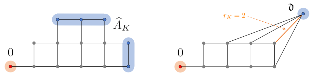
Figure A.1. (Left) graph structure $(\widehat{V}_{K},\,E(\widehat{V}_{K}))$. (Right) graph structure $(V_{K},\,E(V_{K}))$.

In this subsection, we define an auxiliary process which successfully represents the Metropolis dynamics on the edge typical configurations. For $K\geq 5$, we define a graph structure $(\widehat{V}_{K},\,E(\widehat{V}_{K}))$ (see Figure A.1 (left) for an illustration for the case of $K=5$). First, the vertex set $\widehat{V}_{K}\subseteq\mathbb{R}^{2}$ is defined by

$$\widehat{V}_{K}=\{(a,\,b)\in\mathbb{R}^{2}:0\leq b\leq a\leq K\text{ and }b\leq 2\}\setminus\{(K,\,2)\}.$$ (A.1)

Then, the edge structure $E(\widehat{V}_{K})$ is inherited by the Euclidean lattice. We abbreviate by $0=(0,\,0)\in\widehat{V}_{K}$ and define

$$\widehat{A}_{K}=\{(a,\,b)\in\widehat{V}_{K}:a=K\text{ or }b=2\}.$$

Then, we define $\{\widehat{Z}_{K}(t)\}_{t\geq 0}$ as the continuous-time random walk on the aforementioned graph whose transition rate is uniformly $1$. In other words, the transition rate $\widehat{r}_{K}:\widehat{V}_{K}\times\widehat{V}_{K}\rightarrow[0,\,\infty)$ is given by

$$\widehat{r}_{K}(x,\,y)=\begin{cases}1&\text{if }\{x,\,y\}\in E(\widehat{V}_{K}),\\ 0&\text{otherwise}.\end{cases}$$

Obviously, the process is reversible with respect to the uniform distribution on $\widehat{V}_{K}$.

We denote by $\widehat{h}_{\cdot,\cdot}^{K}(\cdot)$ and $\widehat{\mathrm{cap}}_{K}(\cdot,\,\cdot)$ the equilibrium potential and capacity with respect to $\widehat{Z}_{K}(\cdot)$, respectively, in the sense of Definition 3.1. We define a constant $\mathfrak{c}_{K}>0$ by

$$\mathfrak{c}_{K}=|\widehat{V}_{K}|\widehat{\mathrm{cap}}_{K}(0,\,\widehat{A}_{K}).$$ (A.2)

Then, we have the following asymptotic lemma.

Lemma A.1.

There exists a positive constant $\delta$ with $|\delta-0.435|<0.0001$ such that

$$\lim_{K\rightarrow\infty}\mathfrak{c}_{K}=\delta.$$

Proof.

We explicitly compute the equilibrium potential $\widehat{h}_{0,\widehat{A}_{K}}^{K}(\cdot)$. For simplicity, we write $h=\widehat{h}_{0,\widehat{A}_{K}}^{K}$ and abbreviate by $h(a,\,b)=h((a,\,b))$ for $(a,\,b)\in\widehat{V}_{K}$. We define

$$a_{i}=h(K-i,\,0)\;\;\;\;;\;i\in\llbracket 0,\,K\rrbracket\;\;\;\;\text{and}\;\;\;\;b_{i}=h(K-i,\,1)\;\;\;\;;\;i\in\llbracket 0,\,K-1\rrbracket.$$

Then, we trivially have $a_{K}=h(0,\,0)=1$,

$$a_{0}=h(K,\,0)=0\;\;\;\;\text{and}\;\;\;\;b_{0}=h(K,\,1)=0.$$ (A.3)

Moreover, by the Markov property, the following recurrence relations hold:

$$3a_{i} =a_{i+1}+a_{i-1}+b_{i}\;\;\;\;;\;i\in\llbracket 1,\,K-1\rrbracket,$$ (A.4)

$$4b_{i} =b_{i+1}+b_{i-1}+a_{i}\;\;\;\;;\;i\in\llbracket 1,\,K-2\rrbracket,$$ (A.5)

$$2b_{K-1}=b_{K-2}+a_{K-1}\;\;\;\;\text{and}\;\;\;\;3a_{K-1}=1+a_{K-2}+b_{K-1}.$$ (A.6)

Then, (A.4) and (A.5) induce the following relations:

$$a_{i+2}-7a_{i+1}+13a_{i}-7a_{i-1}+a_{i-2} =0\;\;\;;\;i\in\llbracket 2,\,K-3\rrbracket,$$ (A.7)

$$b_{i+2}-7b_{i+1}+13b_{i}-7b_{i-1}+b_{i-2} =0\;\;\;;\;i\in\llbracket 2,\,K-3\rrbracket.$$ (A.8)

Hence, we solve $t^{4}-7t^{3}+13t^{2}-7t+1=0$, which is equivalent to $(t+t^{-1})^{2}-7(t+t^{-1})+11=0$. This gives $t+t^{-1}=(7\pm\sqrt{5})/2$. Thus, we define the positive constants $\alpha_{1},\,\alpha_{2},\,\alpha_{3},\,\alpha_{4}>0$ such that $\alpha_{1}>\alpha_{2}$ are the solutions of $t+t^{-1}=(7+\sqrt{5})/2$ and $\alpha_{3}>\alpha_{4}$ are the solutions of $t+t^{-1}=(7-\sqrt{5})/2$. Then, there exist constants $p_{n}$ and $q_{n}$, $n\in\llbracket 1,\,4\rrbracket$ such that we have, for $i\in\llbracket 0,\,K-1\rrbracket$,

$$a_{i}=\sum_{n=1}^{4}p_{n}\alpha_{n}^{i}\;\;\;\;\text{and}\;\;\;\;b_{i}=\sum_{n=1}^{4}q_{n}\alpha_{n}^{i}.$$ (A.9)

Based on the last formula, (A.3) implies

$$p_{1}+p_{2}+p_{3}+p_{4}=q_{1}+q_{2}+q_{3}+q_{4}=0,$$ (A.10)

and (A.4) implies, for $i\in\llbracket 1,\,K-1\rrbracket$,

$$\sum_{n=1}^{4}\alpha_{n}^{i-1}\{p_{n}\alpha_{n}^{2}-(3p_{n}-q_{n})\alpha_{n}+p_{n}\}=0.$$

As $K\geq 5$, this implies that

$$\begin{bmatrix}1&1&1&1\\ \alpha_{1}&\alpha_{2}&\alpha_{3}&\alpha_{4}\\ \alpha_{1}^{2}&\alpha_{2}^{2}&\alpha_{3}^{2}&\alpha_{4}^{2}\\ \alpha_{1}^{3}&\alpha_{2}^{3}&\alpha_{3}^{3}&\alpha_{4}^{3}\end{bmatrix}\begin{bmatrix}p_{1}\alpha_{1}^{2}-(3p_{1}-q_{1})\alpha_{1}+p_{1}\\ p_{2}\alpha_{2}^{2}-(3p_{2}-q_{2})\alpha_{2}+p_{2}\\ p_{3}\alpha_{3}^{2}-(3p_{3}-q_{3})\alpha_{3}+p_{3}\\ p_{4}\alpha_{4}^{2}-(3p_{4}-q_{4})\alpha_{4}+p_{4}\end{bmatrix}=0.$$

As the square matrix is invertible (cf. Vandermonde matrix), we must have $p_{n}\alpha_{n}^{2}-(3p_{n}-q_{n})\alpha_{n}+p_{n}=0$ for all $n\in\llbracket 1,\,4\rrbracket$, which implies that

$$3p_{n}-q_{n}=\frac{7+\sqrt{5}}{2}p_{n}\;\;\;\;;\;n=1,\,2,\;\;\;\;\text{and}\;\;\;\;3p_{n}-q_{n}=\frac{7-\sqrt{5}}{2}p_{n}\;\;\;\;;\;n=3,\,4.$$

Hence, substituting (A.10) and the last display to (A.9) gives, for $i\in\llbracket 0,\,K-1\rrbracket$,

$$a_{i}=p_{1}(\alpha_{1}^{i}-\alpha_{2}^{i})+p_{3}(\alpha_{3}^{i}-\alpha_{4}^{i}),\;\;\;b_{i}=-\frac{1+\sqrt{5}}{2}p_{1}(\alpha_{1}^{i}-\alpha_{2}^{i})+\frac{-1+\sqrt{5}}{2}p_{3}(\alpha_{3}^{i}-\alpha_{4}^{i}).$$ (A.11)

Substituting the last formula to (A.6) implies

$$(2+\sqrt{5})p_{1}(\alpha_{1}^{K-1}-\alpha_{2}^{K-1})+(2-\sqrt{5})p_{3}(\alpha_{3}^{K-1}-\alpha_{4}^{K-1})$$

$$=\frac{1+\sqrt{5}}{2}p_{1}(\alpha_{1}^{K-2}-\alpha_{2}^{K-2})+\frac{1-\sqrt{5}}{2}p_{3}(\alpha_{3}^{K-2}-\alpha_{4}^{K-2})$$

and

$$\frac{7+\sqrt{5}}{2}p_{1}(\alpha_{1}^{K-1}-\alpha_{2}^{K-1})+\frac{7-\sqrt{5}}{2}p_{3}(\alpha_{3}^{K-1}-\alpha_{4}^{K-1})$$

$$=1+p_{1}(\alpha_{1}^{K-2}-\alpha_{2}^{K-2})+p_{3}(\alpha_{3}^{K-2}-\alpha_{4}^{K-2}).$$

Solving the last two equations, we can express $p_{1}$ and $p_{3}$ in terms of $\alpha_{1},\,\alpha_{2},\,\alpha_{3},\,\alpha_{4}$. Substituting these to the first equation of (A.11) for $i=K-1$, we deduce that $a_{K-1}$ equals

$$-\Big{[}(2-\sqrt{5})-\frac{1-\sqrt{5}}{2}\frac{\alpha_{3}^{K-2}-\alpha_{4}^{K-2}}{\alpha_{3}^{K-1}-\alpha_{4}^{K-1}}\Big{]}+\Big{[}(2+\sqrt{5})-\frac{1+\sqrt{5}}{2}\frac{\alpha_{1}^{K-2}-\alpha_{2}^{K-2}}{\alpha_{1}^{K-1}-\alpha_{2}^{K-1}}\Big{]}$$

divided by

$$\Big{[}(2+\sqrt{5})-\frac{1+\sqrt{5}}{2}\frac{\alpha_{1}^{K-2}-\alpha_{2}^{K-2}}{\alpha_{1}^{K-1}-\alpha_{2}^{K-1}}\Big{]}\Big{[}\frac{7-\sqrt{5}}{2}-\frac{\alpha_{3}^{K-2}-\alpha_{4}^{K-2}}{\alpha_{3}^{K-1}-\alpha_{4}^{K-1}}\Big{]}$$

$$-\Big{[}(2-\sqrt{5})-\frac{1-\sqrt{5}}{2}\frac{\alpha_{3}^{K-2}-\alpha_{4}^{K-2}}{\alpha_{3}^{K-1}-\alpha_{4}^{K-1}}\Big{]}\Big{[}\frac{7+\sqrt{5}}{2}-\frac{\alpha_{1}^{K-2}-\alpha_{2}^{K-2}}{\alpha_{1}^{K-1}-\alpha_{2}^{K-1}}\Big{]}.$$

As $\alpha_{1}>\alpha_{2}$ and $\alpha_{3}>\alpha_{4}$, we have $(\alpha_{2}/\alpha_{1})^{K-1}\rightarrow 0$ and $(\alpha_{4}/\alpha_{3})^{K-1}\rightarrow 0$ as $K\rightarrow\infty$. Thus, we may calculate

$$\lim_{K\rightarrow\infty}a_{K-1} =\frac{-\Big{[}(2-\sqrt{5})-\frac{1-\sqrt{5}}{2}\frac{1}{\alpha_{3}}\Big{]}+\Big{[}(2+\sqrt{5})-\frac{1+\sqrt{5}}{2}\frac{1}{\alpha_{1}}\Big{]}}{\Big{[}(2+\sqrt{5})-\frac{1+\sqrt{5}}{2}\frac{1}{\alpha_{1}}\Big{]}\Big{[}\frac{7-\sqrt{5}}{2}-\frac{1}{\alpha_{3}}\Big{]}-\Big{[}(2-\sqrt{5})-\frac{1-\sqrt{5}}{2}\frac{1}{\alpha_{3}}\Big{]}\Big{[}\frac{7+\sqrt{5}}{2}-\frac{1}{\alpha_{1}}\Big{]}}$$

$$=\frac{2\sqrt{5}-\frac{1+\sqrt{5}}{2}\alpha_{2}+\frac{1-\sqrt{5}}{2}\alpha_{4}}{5\sqrt{5}+\frac{3-5\sqrt{5}}{2}\alpha_{2}+\frac{-3-5\sqrt{5}}{2}\alpha_{4}+\sqrt{5}\alpha_{2}\alpha_{4}}.$$

In the second equality, we used that $\alpha_{1}\alpha_{2}=\alpha_{3}\alpha_{4}=1$. By substituting the exact values of $\alpha_{i}$, this is asymptotically $0.5649853624$. Moreover, as $0=(0,\,0)\in\widehat{V}_{K}$ is connected only to $(1,\,0)\in\widehat{V}_{K}$, we have by [5, (7.1.39)] that

$$\widehat{\mathrm{cap}}_{K}(0,\,\widehat{A}_{K})=\frac{1}{|\widehat{V}_{K}|}[h(0,\,0)-h(1,\,0)]=\frac{1-a_{K-1}}{|\widehat{V}_{K}|}.$$

Therefore, we have

$$\lim_{K\rightarrow\infty}\mathfrak{c}_{K}=\lim_{K\rightarrow\infty}|\widehat{V}_{K}|\widehat{\mathrm{cap}}_{K}(0,\,\widehat{A}_{K})=1-\lim_{K\rightarrow\infty}a_{K-1}\approx 0.4350146376,$$

which concludes the proof. ∎

Remark A.2.

In the periodic boundary case, we need a completely different auxiliary process to estimate the structure of edge typical configurations. Namely, the desired process is a Markov chain on the collection of subtrees of a $K\times 2$-shaped ladder graph with semi-periodic boundary conditions (i.e., open on the horizontal boundaries and periodic on the vertical ones). In this case, we deduce an upper bound for the corresponding capacity, which is sufficient to obtain the bound (9.3). We refer to [14, Proposition 7.9] for more information on this estimate.

A.2. Projected auxiliary process

Based on the original auxiliary process defined in the preceding subsection, we define a projected auxiliary process which is obtained by simply projecting the elements in $\widehat{A}_{K}$ to a single element $\mathfrak{d}$. Rigorously, we define a graph structure $(V_{K},\,E(V_{K}))$ (see Figure A.1 (right) for an illustration for the case of $K=5$). The vertex set $V_{K}\subseteq\mathbb{R}^{2}$ is defined by

$$V_{K}=(\widehat{V}_{K}\setminus\widehat{A}_{K})\cup\{\mathfrak{d}\}.$$ (A.12)

Then, the edge structure $E(V_{K})$ is inherited by $E(\widehat{V}_{K})$; we have $\{x,\,y\}\in E(V_{K})$ for $\{x,\,y\}\in E(\widehat{V}_{K})$, $x,\,y\in\widehat{V}_{K}\setminus\widehat{A}_{K}$, and we have $\{x,\,\mathfrak{d}\}\in E(V_{K})$ for

$$x\in\widehat{V}_{K}\setminus\widehat{A}_{K}\;\;\;\;\text{satisfying}\;\;\;\;\exists y\in\widehat{A}_{K}\;\;\;\;\text{with}\;\;\;\;\{x,\,y\}\in E(\widehat{V}_{K}).$$

Then, we define $\{Z_{K}(t)\}_{t\geq 0}$ as the continuous-time Markov chain on $(V_{K},\,E(V_{K}))$ whose transition rate $r_{K}$ is defined by $r_{K}(x,\,y)=\widehat{r}_{K}(x,\,y)$ if $x,\,y\neq\mathfrak{d}$ and

$$r_{K}(x,\,\mathfrak{d})=r_{K}(\mathfrak{d},\,x)=\sum_{y\in\widehat{A}_{K}}\widehat{r}_{K}(x,\,y).$$

This process is reversible with respect to the uniform distribution on $V_{K}$.

We denote by $h_{\cdot,\cdot}^{K}(\cdot)$, $\mathrm{cap}_{K}(\cdot,\,\cdot)$, $D_{K}(\cdot)$ the equilibrium potential, capacity, and Dirichlet form with respect to $Z_{K}(\cdot)$, respectively, in the sense of Definition 3.1. Then, by the strong Markov property, it is immediate from the definition that

$$h_{0,\mathfrak{d}}^{K}(x)=\widehat{h}_{0,\widehat{A}_{K}}^{K}(x)\;\;\;\;;\;x\in\widehat{V}_{K}\setminus\widehat{A}_{K}\;\;\;\;\text{and}\;\;\;\;h_{0,\mathfrak{d}}^{K}(\mathfrak{d})=\widehat{h}_{0,\widehat{A}_{K}}^{K}(y)=0\;\;\;\;;\;y\in\widehat{A}_{K}.$$

Therefore, by (3.4), we have (cf. (A.2))

$$|V_{K}|\mathrm{cap}_{K}(0,\,\mathfrak{d})=|\widehat{V}_{K}|\widehat{\mathrm{cap}}_{K}(0,\,\widehat{A}_{K})=\mathfrak{c}_{K}.$$ (A.13)

Acknowledgement.

S. Kim was supported by NRF-2019-Fostering Core Leaders of the Future Basic Science Program/Global Ph.D. Fellowship Program and the National Research Foundation of Korea (NRF) grant funded by the Korean government (MSIT) (No. 2018R1C1B6006896).

References

• [1] Beltrán, J.; Landim, C.: Tunneling and metastability of continuous time Markov chains. Journal of Statistical Physics. 140: 1065-1114. (2010)
• [2] Beltrán, J.; Landim, C.: Tunneling and metastability of continuous time Markov chains II, the nonreversible case. Journal of Statistical Physics. 149: 598-618. (2012)
• [3] Beltrán, J.; Landim, C.: A martingale approach to metastability. Probability Theory and Related Fields. 161: 267-307. (2015)
• [4] Ben Arous, G.; Cerf, R.: Metastability of the three dimensional Ising model on a torus at very low temperatures. Electronic Journal of Probability. 1: 1-55. (1996)
• [5] Bovier, A.; den Hollander, F.: Metastabillity: A Potential-theoretic approach. Grundlehren der mathematischen Wissenschaften. Springer. (2015)
• [6] Bovier, A.; Eckhoff, M.; Gayrard, V.; Klein, M.: Metastability in reversible diffusion processes I. Sharp asymptotics for capacities and exit times. Journal of the European Mathematical Society. 6: 399-424. (2004)
• [7] Cassandro, M.; Galves, A.; Olivieri, E.; Vares, M.E.: Metastable behavior of stochastic dynamics: A pathwise approach. Journal of Mathematical Physics. 35: 603-634. (1984)
• [8] Cirillo, E.N.M.; Nardi, F.R.: Relaxation height in energy landscapes: An application to multiple metastable states. Journal of Statistical Physics. 150: 1080-1114. (2013)
• [9] Cirillo, E.N.M.; Nardi, F.R.; Spitoni, C.: Sum of exit times in a series of two metastable states. The European Physical Journal Special Topics. 226: 2421-2438. (2017)
• [10] Cirillo, E.N.M.; Olivieri, E.: Metastability and nucleation for the Blume–Capel model. Different mechanisms of transition. Journal of Statistical Physics. 83: 473-554. (1996)
• [11] Gaudillière, A.; Landim, C.: A Dirichlet principle for non reversible Markov chains and some recurrence theorems. Probability Theory and Related Fields. 158: 55-89. (2014)
• [12] Kim, S.: Second time scale of the metastability of reversible inclusion processes. Probability Theory and Related Fields. https://doi.org/10.1007/s00440-021-01036-6 (2021)
• [13] Kim, S.; Seo, I.: Condensation and metastable behavior of non-reversible inclusion processes. Communications in Mathematical Physics. 382: 1343-1401. (2021)
• [14] Kim, S.; Seo, I.: Metastability of stochastic Ising and Potts models on lattices without external fields. arXiv:2102.05565 (2021)
• [15] Landim, C.; Lemire, P.: Metastability of the two-dimensional Blume–Capel model with zero chemical potential and small magnetic field. Journal of Statistical Physics. 164: 346-376. (2016)
• [16] Landim, C.; Lemire, P.; Mourragui, M.: Metastability of the two-dimensional Blume–Capel model with zero chemical potential and small magnetic field on a large torus. Journal of Statistical Physics. 175: 456-494. (2019)
• [17] Landim, C.; Marcondes, D.; Seo, I.: A resolvent approach to metastability. arXiv:2102.00998 (2021)
• [18] Landim, C.; Mariani, M.; Seo, I.: Dirichlet’s and Thomson’s principles for non-selfadjoint elliptic operators with application to non-reversible metastable diffusion processes. Archive for Rational Mechanics and Analysis. 231: 887-938. (2019)
• [19] Levin, D.A.; Peres, Y.; Wilmer, E.L.: Markov Chains and Mixing Times. American Mathematical Society. (2017)
• [20] Manzo, F.; Olivieri, E.: Dynamical Blume–Capel model: Competing metastable states at infinite volume. Journal of Statistical Physics. 104: 1029-1090. (2001)
• [21] Nardi, F.R.; Zocca, A.: Tunneling behavior of Ising and Potts models in the low-temperature regime. Stochastic Processes and their Applications. 129: 4556-4575. (2019)
• [22] Nardi, F.R.; Zocca, A.; Borst, S.C.: Hitting time asymptotics for hard-core interactions on grids. Journal of Statistical Physics. 162: 522-576. (2016)
• [23] Neves, E.J.; Schonmann, R.H.: Critical droplets and metastability for a Glauber dynamics at very low temperatures. Communications in Mathematical Physics. 137: 209-230. (1991)
• [24] Olivieri, E.; Vares, M.E.: Large deviations and metastability. Encyclopedia of Mathematics and Its Applications, vol. 100. Cambridge University Press, Cambridge. (2005)
• [25] Rezakhanlou, F.; Seo, I.: Scaling limit of small random perturbation of dynamical systems. arXiv:1812.02069 (2018)
• [26] Seo, I.: Condensation of non-reversible zero-range processes. Communications in Mathematical Physics. 366: 781-839. (2019)