On a Mathematical model for traveling
sand dune

Abstract.

Our aim in this paper is to introduce and study a mathematical model for the description of traveling sand dunes. We use surface flow process of sand under the effect of wind and gravity. We model this phenomena by a non linear diffusion-transport equation coupling the effect of transportation of sand due to the wind and the avalanches due to the gravity and the repose angle. The avalanche flow is governed by the evolution surface model and we use a nonlocal term to handle the transport of sand face to the wind.

1. Introduction

The diffusion-transport equation of the type

$$\partial_{t}u=\nabla\cdot\Big{(}m\>\nabla u-V\>u\Big{)}+f$$ (1)

governs the spatio-temporal dynamics of a density $\displaystyle u(x,t)$ of particles. The first term on the right hand side describes random motion and the parameter $\displaystyle m$, corresponding to diffusion coefficient, is connected to rate of random exchanges between the particles at the position $\displaystyle x$ and neighbors positions. The second term is a transportation with velocity $\displaystyle V,$ and is connected to the transport of particles according to the the vector field $\displaystyle V.$

Our aim here is to show how one can use this type of equation to describe the movement of traveling sand dunes ; the so called Barchans. A Barchan is a dune of the shape of a crescent lying in the direction of the wind. It arises where the supply of sand is low and under unidirectional winds. The wind rolled the sand back to the slope of the dune back up the ridge and comes to cause small avalanches on steep slopes over the front. This furthered the dune. Such dunes (Barchan) move in the desert at speeds depending on their size and strength of wind. In one year, they argue a few meters to a few tens of meters. A wind of $\displaystyle\displaystyle 25km/h$ is enough to turn on the preceding process and furthered the dune. Our main is to show how one can couple between the action of the wind and the action of gravity into the equation (1) to fashion a model for traveling sand dunes like Barchans.

Recall that the surface evolution model is a very useful model for the description of the dynamic of a granular matter under the gravity effect. In [30] (see also [4], and [14]) the authors show that this toy model gives a simple way to study the dynamic of the sandpile from the theoretical and a numerical point of view. In particular, the connection of this model with a stochastic model for sandpile (cf. [18]) shows how it is able to handle the global dynamic of a structure of granular matter structure using simply the repose angle. In this paper, we show how one can use the surface evolution model in the equation (1) to describe the dynamic of traveling sand dunes. There is a wide literature concerning mathematical and physical studies of dunes (cf. [5], [25], [2, 3], [32] and [26]). We do believe that this is an intricate phenomena with many determinant parameters. We are certainly neglecting some of them. Nevertheless, as for the case of sandpile, we do believe that simple models (like toys model) may help to encode complex phenomenon related to the granular matter structures.

In the following section, we give some preliminaries and present our model for a traveling sand dune. Section 3 is devoted main results of existence and uniqueness of a weak solution.

2. Preliminaries and modeling

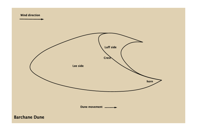
Figure 1. Barchan

The simplest and the most well-known type of dunes is the Barchan. In general, it has the form of a hill with a Luff side and a Lee side separated by a crest (cf. Figure 1). On the Lee side, sand is taken up by the wind into a moving layer, transported up to the crest and pass to the other side; the Luff side. By neglecting the effects of precipitation and swirls, on the Luff side, the dynamic of the sand is generated by the action of gravity on the sand arriving at the crest.

Though there are many speculations and experimental observations on the evolution of the shape, the height and the distribution of dunes, there is no universal model for the study of the motion of sand dunes. There is a large literature on this subject (cf. [5], [25], [2, 3], [32] and [26]). Some mathematical models treats the dunes as an aerodynamic objects with an adequate smooth shape to let the air flow by with the least effort (cf. [25]). The so called BCRE models (cf. [27]) use the conservation of mass and the repose angle to build a system of two coupled differential equations for the height of the topography $\displaystyle h$ and the amount of mobile particles $\displaystyle R.$ The particles are supposed to move all with the same velocity $\displaystyle u.$ Other simplified and realistic physical models (cf. [2, 3], [32] and [26]) use the mass and momentum conservation in presence of erosion and external forces to derive coupled differential equations to study the evolution of the morphology of dunes. Among other things, these models focus on the way in which a sand movement could be constructed from wind data (the choice of formula for linking wind velocity to sand movement, the choice of a threshold velocity for sand movement e.g. Bagnold, etc). Keeping in mind that the driving force for the Barchans is the wind, our aim here is to introduce and study a simple model which combines the effort of wind on the Lee side with the avalanches generated by the repose angle. More precisely, we introduce and study a new mathematical model in the form of diffusion-transport equation (1) for the evolution of a morphology of a Barchan under the effect of a unidirectional wind.

Let us denote by $\displaystyle u=u(t,x,y)$ the height of the dune at time $\displaystyle t\geq 0$ and at the position $\displaystyle\displaystyle(x,y)$ in the plane $\displaystyle\mathbb{R}^{N}$ ($\displaystyle N=2$ in practice). Then, $\displaystyle u$ can be described by (1) where the term $\displaystyle-m\>\nabla u$ is connected to the net flux of the avalanches of sands resulting from the action of the gravity and the repose angle. The term $\displaystyle uV$ is connected to the transport of the sand under the action of wind up to the crest. See here that $\displaystyle f\equiv 0$, since we are assuming that there is no source of sand. Thanks to [30] (see also [4] and [18]) we know that the avalanche can be governed by a non standard diffusion parameter $\displaystyle m$ (unknown) that is connected to the sub-gardient constraint in the following way

$$m\geq 0,\ |\nabla u|\leq\lambda,\ m\>(|\nabla u|-\lambda)=0,$$

where $\displaystyle\theta=\arctan(\lambda)$ is the repose angle of the sand. This is the consequence of the fact that the inertia is neglected, the surface flow is directed towards the steepest descent, the surface slope of the sandpile cannot exceed the repose angle $\displaystyle\theta$ of the material and there is no pouring over the parts of angle less than $\displaystyle\theta.$ As to the action of the wind, the resulting phenomena is a transportation of $\displaystyle u$ in the direction of the wind. Indeed, the wind proceed by taking up the sand into a moving layer and transport it up to the crest. This creates a ripping curent of sand concentrated in the Lee side ; face up the wind. To handle the way a sand movement could be constructed from wind data, we use the nonlocal interactions between the positions of the dune face to the wind. We assume that the velocity $\displaystyle V=(V_{1},0)$ of the transported layer is induced at a site $\displaystyle x$ by the net effects of the slope of all particles at various sites $\displaystyle y$ around $\displaystyle x.$ More precisely, we consider $\displaystyle V_{1}$ in the form

$$V_{1}=\mathcal{H}(K\star\partial_{x}u)=\mathcal{H}\left(\int_{B(x,r)}K(x-y)\>\partial_{x}u(y,t)\>dy\right),$$

where the kernel $\displaystyle K$ associates a strength of interaction per unit density with the distance $\displaystyle x-y$ between any two sites over some finite domain $\displaystyle B(x,r).$ Taking the average of this form may give more weight to information about particles that are closer, or those that are farther away. Moreover, since the transport need to be restricted to the region facing the wind, we assume that the function, $\displaystyle\mathcal{H}\>:\>\mathbb{R}\to\mathbb{R}^{+}$ is a phenomenological parameter which vanishes in the region $\displaystyle(-\infty,0).$

Thus, we consider the following model to describe the evolution of the morphology of a Barchan under the effect of a unidirectional wind (in the direction $\displaystyle(1,0)$) :

$$\left\{\begin{array}[]{ll}\left.\begin{array}[]{l}\displaystyle\partial_{t}u-\nabla\cdot({m}\>\nabla u)+\partial_{x}\Big{(}u\>\mathcal{H}(K\star\partial_{x}u)\Big{)}=0\\ \\ \displaystyle|\nabla u|\leq\lambda,\ {m}\geq 0,\ {m}\>(|\nabla u|-\lambda)=0\end{array}\right\}&\quad\hbox{ in }(0,\infty)\times\mathbb{R}^{N}\\ \\ u(0,x)=u_{0}(x)&\quad\hbox{ for }x\in\mathbb{R}^{N}.\end{array}\right.$$ (2)

Remark 2.1.

1. In (2), we are assuming that the flux du to the wind ; i.e. the quantity of sand transported by unit of time through fixed vertical line, depends on the speed of the wind and the angle of the position. Moreover, thanks to the assumption on $\displaystyle\mathcal{H}$ (vanishing in $\displaystyle(-\infty,0)$), the action of the wind is null whenever the slope is not face to the wind. To be more general, it is possible to assume that this flux depends also on the eight, i.e. we can assume that

   $$V_{1}=\>\beta(u)\>\mathcal{H}(K\star\partial_{x}u),$$

   where $\displaystyle\displaystyle\beta\>:\>\mathbb{R}^{+}\to\mathbb{R}^{+}$ is a continuous function.

2. We see in the formal model (2) that $\displaystyle\mathcal{H}$ is null for negative values and strictly positive on $\displaystyle\mathbb{R}^{+}.$ So, formally, $\displaystyle\mathcal{H}=\chi_{\mathbb{R}^{+}}.$ Here, for technical reason, we consider continuous approximation of this kind of profile by assuming that $\displaystyle\mathcal{H}$ is a Lipschitz continuous function on $\displaystyle\mathbb{R}$. For instance, one can take

   $$\displaystyle\mathcal{H}(r)=1-\frac{1}{\sqrt{\pi}}\int^{-r/\sqrt{\varepsilon}}_{-1/\varepsilon}e^{-z^{2}}dz,$$

   where $\displaystyle 0<\varepsilon<1$ is a given fixed parameter .

3. Since the assumptions on $\displaystyle\mathcal{H},$ one sees that the crest, which corresponds here to the region where $\displaystyle u$ changes its monotonicity, constitutes a free boundary separating the region of avalanches and the region of wind erosion of sand. Indeed, the transport term $\displaystyle uV$ disappears in the region where $\displaystyle u$ is nonincreasing.

4. It is possible to improve the property of $\displaystyle\mathcal{H}$ to better describe the movement of sand face the wind. For instance if we assume that the grains move more and more slowly whenever they are face to important slope, then $\displaystyle\mathcal{H}$ can be assumed to be a nondecreasing Lipschitz continuous function. Typical example may be given by

   $$\mathcal{H}(r)=\frac{r^{+}}{\sqrt{1+r^{2}}},\quad\hbox{ for any }r\in\mathbb{R}.$$

   In this paper, we just assume that $\displaystyle\mathcal{H}$ is a Lipschitz continuous function. The discussions concerning concrete assumptions on $\displaystyle\mathcal{H}$ and also on $\displaystyle\gamma$ and $\displaystyle K$ will be discussed in forthcoming papers.

5. Replacing $\displaystyle K$ by $\displaystyle K_{\sigma}$ in (2) where $\displaystyle K_{\sigma}\in\mathcal{D}(\mathbb{R}^{N})$ is a smoothing kernel satisfying

   • $\displaystyle\displaystyle\int_{\mathbb{R}^{N}}K_{\sigma}(x)\>dx=1$

   • $\displaystyle\displaystyle K_{\sigma}(x)\to\delta_{x}$ as $\displaystyle\sigma\to 0$, $\displaystyle\delta_{x}$ is the Dirac function at the point $\displaystyle x$,

   and letting formally $\displaystyle\sigma\to 0$ in (2), we obtain the following PDE :

   $$\left\{\begin{array}[]{ll}\left.\begin{array}[]{l}\displaystyle\partial_{t}u-\nabla\cdot({m}\>\nabla u)+\partial_{x}\Big{(}\gamma(u)\>\mathcal{H}(\partial_{x}u)\Big{)}=0\\ \\ \displaystyle|\nabla u|\leq\lambda,\ \exists\ {m}\geq 0,\ {m}\>(|\nabla u|-\lambda)=0\end{array}\right\}&\quad\hbox{ in }(0,\infty)\times\mathbb{R}^{N}\\ \\ u(0,x)=u_{0}(x)&\quad\hbox{ for }x\in\mathbb{R}^{N}.\end{array}\right.$$ (3)

   Since $\displaystyle\mathcal{H}$ is assumed to be nondecreasing, one sees that the term $\displaystyle\partial_{x}\Big{(}\gamma(u)\>\mathcal{H}(\partial_{x}u)\Big{)}$ is a anti-diffusive and may creates some obstruction to the existence of a solution. It is not clear for us if (3) is well posed in this case or not.

3. Existence and uniqueness

To study the model (2), we restrict our-self to $\displaystyle\Omega\subset\mathbb{R}^{N}$ a bounded open domain, with Lipschitz boundary $\displaystyle\partial\Omega$ and outer unit normal $\displaystyle\eta$. Consider the following nonlocal equation with Dirichlet boundary condition :

$$\begin{array}[]{ll}\left.\begin{array}[]{l}\displaystyle\partial_{t}u-\nabla\cdot({m}\>\nabla u)+\partial_{x}\Big{(}\gamma(u)\>\mathcal{H}(K\star\partial_{x}u)\Big{)}=f\\ \\ \displaystyle|\nabla u|\leq\lambda,\ \exists\ {m}\geq 0,\ {m}\>(|\nabla u|-\lambda)=0\end{array}\right\}&\mbox{ in}\,\Omega_{T}:=(0,T)\times\Omega\\ \\ u=0&\mbox{ in}\,\,\Sigma_{T}:=(0,T)\times\partial\Omega\\ \\ u(0,x)=u_{0}(x)&\mbox{ in}\,\,\Omega,\end{array}\right.$$

where $\displaystyle u_{0}$ patterns the intial shape of the dune. Here and throughout the paper, we assume that

• $\displaystyle\mathcal{H}\>:\>\mathbb{R}\to\mathbb{R}^{+}$ is a Lipschitz continuous function.

• $\displaystyle K$ is a given regular Kernel compactly supported in $\displaystyle B(0,r),$ for a given parameter $\displaystyle r>0.$

• $\displaystyle\displaystyle\gamma\>:\>\mathbb{R}^{+}\to\mathbb{R}^{+}$ is a Lipschitz continuous function with $\displaystyle\displaystyle\gamma(0)=0$.

Our main results concerns existence and uniqueness of a solution. As usual for the first differential operator governing the PDE (E), we use the notion of variational solution. We consider $\displaystyle\mathcal{C}_{0}(\Omega),$ the set of continuous function null on the boundary. For any $\displaystyle 0\leq\alpha\leq 1,$ we consider

$$\displaystyle\mathcal{C}_{0}^{0,\alpha}(\Omega)=\Big{\{}u\in\mathcal{C}_{0}(\Omega)\>:\>u(x)-u(y)\leq C|x-y|^{\alpha}\hbox{ for any }x,y\in\overline{\Omega}\Big{\}},$$

endowed with the natural norm

$$\|u\|_{\mathcal{C}_{0}^{0,\alpha}(\Omega)}=\sup_{x\in\Omega}|u(x)|+\sup_{x\neq y\in\Omega}\frac{|u(x)-u(y)|}{|x-y|^{\alpha}}.$$

We denote by

$$Lip=\mathcal{C}^{0,1}(\Omega)\quad\hbox{ and }Lip_{0}=Lip\cap\mathcal{C}_{0}(\Omega).$$

Then, we denote by

$$\displaystyle Lip_{1}=\Big{\{}u\in\mathcal{C}_{0}(\Omega)\>:\>u(x)-u(y)\leq|x-y|\hbox{ for any }x,y\in\Omega\Big{\}}.$$

The topological dual space of $\displaystyle Lip_{0}$ will be denoted by $\displaystyle Lip^{*}_{0}$ and is endowed with the natural dual norm, and we denote by $\displaystyle\langle.,.\rangle$ the duality bracket. It is clear that, for any $\displaystyle\xi\in Lip_{1},$ we have

$$|\xi(x)|\leq\delta_{\Omega},\quad\hbox{ for any }x\in\Omega,$$

where $\displaystyle\delta_{\Omega}$ denotes the diameter of the domain $\displaystyle\Omega.$

Recall that the notion of solution for the problems of the type ($(E)\{$) is not standard in general. The problem presents two specific difficulties. The first one is related to the main operator governing the equation : $\displaystyle-\nabla\cdot(m\nabla u)$ with $\displaystyle m\geq 0$ and $\displaystyle m(|\nabla u|-1)=0$. And the second one is connected to the regularity of the term $\displaystyle\partial_{t}u$.

Concerning the main operator governing the equation recall that $\displaystyle u$ is Lipschitz and, in general even in the case where $\displaystyle\mathcal{H}\equiv 0,$ $\displaystyle m$ is singular. So, the term $\displaystyle m\nabla u$ is not well defined in general and needs to be specified. To handle the PDE with the operator in divergence form request the use of the notion of tangential gradient with respect to a measure (cf. [8, 9, 10]). Nevertheless, to avoid all the technicality related to this approach, we use here the notion of truncated-variational solution (that we call simply variational solution) to handle the problem. Indeed, the following lemma strips the way to this alternative. For any $\displaystyle k>0,$ the real function $\displaystyle T_{k}$ denotes the usual truncation given by

$$T_{k}(r)=\max(\min(r,k),-k),\quad\hbox{ for any }r\in\mathbb{R}.$$ (4)

Lemma 3.1.

Let $\displaystyle\eta\in Lip^{*}_{0}$ and $\displaystyle u\in Lip_{1}.$ If, there exists $\displaystyle m\in L^{1}(\Omega)$ such that $\displaystyle m\geq 0$, $\displaystyle m(|\nabla u|-1)=0$ a.e. in $\displaystyle\Omega$ and $\displaystyle\nabla\cdot(m\nabla u)=\eta$ in $\displaystyle\mathcal{D}^{\prime}(\Omega),$ then,

$$\langle\eta,T_{k}(u-\xi)\rangle\geq 0,\quad\hbox{ for any }\xi\in Lip_{1}\hbox{ and }k>0.$$

The proof of this lemma is simple, we let it as an exercise for the interested reader. Let us notice that the converse part remains true if one take on $\displaystyle m$ to be a measure and the gradient to be the tangential gradient with respect to $\displaystyle m.$ Other equivalent formulations may be found in [20].

This being said, one sees that performing the notion of variational solution in (E) generates formally the quantity $\displaystyle\langle u_{t},T_{k}(u-\xi)\rangle.$ Since in general $\displaystyle\partial_{t}u$ is not necessary a Lebesgue function we process the following (formal) integration by parts formula in the definition of the solution :

$$\langle\partial_{t}u,T_{k}(u-\xi)\rangle=\frac{d}{dt}\int_{\Omega}\int_{0}^{u(t)}T_{k}(s-\xi)dsdx.$$

Observe that, letting $\displaystyle k\to\infty,$ the last formula turns into

$$\langle\partial_{t}u,u-\xi\rangle=\frac{1}{2}\frac{d}{dt}\int_{\Omega}|u-\xi|^{2}\>dx.$$

This is the common term for the standard notion of variational solution. It is noteworthy, however, that the truncation operation here is an important ingredient to get uniqueness (see the uniqueness proof and the remark below).

The considerations above bring on the following definition of variational solutions :

Definition 3.2.

Let $\displaystyle\displaystyle f\in L^{1}(\Omega_{T})$ and $\displaystyle u_{0}\in Lip_{1}.$ A variational solution of (E) is a function $\displaystyle u\in L^{\infty}(0,T,C_{0}(\Omega))$ such that $\displaystyle u(t)\in Lip_{1}$ for a.e. $\displaystyle t\in[0,T]$, and for every $\displaystyle\xi\in Lip_{1}$ and every $\displaystyle k>0$,

$$\frac{d}{dt}\int_{\Omega}\int_{0}^{u(t)}T_{k}(s-\xi)ds{d}x-\int_{\Omega}\gamma(u)\>\mathcal{H}(\partial_{x}K\ast u)\partial_{x}T_{k}(u-\xi)dx\leq\int_{\Omega}f\>T_{k}(u-\xi)\>dx$$ (5)

in $\displaystyle\mathcal{D}^{\prime}([0,T)).$

In other words, $\displaystyle u\in L^{\infty}((0,T),C^{0}(\Omega))$ such that $\displaystyle u(t)\in Lip_{1}$ for a.e. $\displaystyle t\in[0,T]$ is a variational solution of (E) if for every $\displaystyle\xi\in Lip_{1}$ and every $\displaystyle\sigma\in C^{1}([0,T),\mathbb{R}_{+})$ one has

$$-\int_{0}^{T}\!\!\!\int_{\Omega}\dot{\sigma}(t)\int_{0}^{u(t)}T_{k}(s-\xi)dsdxdt-\int_{0}^{T}\!\!\!\int_{\Omega}{\sigma}(t)\gamma(u(t))\>\mathcal{H}(\partial_{x}K\ast)\partial_{x}T_{k}(u(t)-\xi)dxdt$$

$$\leq\sigma(0)\int_{\Omega}\int_{0}^{u_{0}}T_{k}(s-\xi)dsdx+\int_{0}^{T}\!\!\!\int_{\Omega}\sigma(t)f(t)\>T_{k}(u(t)-\xi)dtdx.$$

Remark 3.3.

1. It is achievable to define a solution as a function $\displaystyle u\in L^{\infty}((0,T),C^{0}(\Omega))$, with $\displaystyle\partial_{t}u\in L^{1}(0,T;Lip^{*}_{0})$ and $\displaystyle u(t)\in Lip_{1}$ for a.e. $\displaystyle t\in[0,T]$, $\displaystyle u(0)=u_{0}$ and

   $$\begin{array}[]{c}\langle\partial_{t}u,T_{k}(u-\xi)\rangle-\int_{\Omega}\gamma(u)\>\mathcal{H}(\partial_{x}K\ast u)\partial_{x}T_{k}(u-\xi)dx\\ \leq\int_{\Omega}f\>T_{k}(u-\xi)\>dx,\quad\hbox{ for a.e. }t\in(0,T),\end{array}$$ (6)

   where $\displaystyle\langle.,.\rangle$ denote sthe duality brackect in $\displaystyle Lip^{*}_{0}.$ However, one can prove that if $\displaystyle u$ satisfies (6) it is also a variational solution in the sense of Definition 3.2. Indeed, if $\displaystyle\partial_{t}u\in L^{1}(0,T;Lip^{*}_{0})$ one can prove rigorously that (6) yields

   $$\int_{0}^{T}\langle\partial_{t}u(t),T_{k}(u(t)-\xi)\rangle\sigma(t)\>dt=-\int_{0}^{T}\int_{\Omega}\dot{\sigma}(t)\int_{0}^{u(t)}T_{k}(s-\xi)dsdxdt$$

   $$-\sigma(0)\int_{\Omega}\int_{0}^{u_{0}}T_{k}(s-\xi)dsdx,$$

   for any $\displaystyle\xi\in Lip_{1}$ and $\displaystyle\sigma\in C^{1}([0,T),\mathbb{R}).$

2. Notice that some similar notion of solution have been used in [AgCaIg] for a different problem using the so called W1-JKO scheme, where W1 is related to the Wasserstein distance $\displaystyle W_{1}.$

Theorem 3.4.

Let $\displaystyle\displaystyle f\in L^{1}(\Omega_{T})$ and $\displaystyle u_{0}\in Lip_{1}.$ The problem (E) has a unique variational solution $\displaystyle u$.

To prove this theorem, we see that Lemma 3.1 implies that the operator $\displaystyle u\in Lip_{1}\to-\nabla\cdot(m\nabla u)$, with non-negative $\displaystyle m$ satisfying $\displaystyle m(|\nabla u|-1)=0,$ may be represented in $\displaystyle L^{2}(\Omega),$ by the sub-differential operator $\displaystyle\partial\displaystyle\mathbbm{I}_{{Lip_{1}}}$ of the indicator function $\displaystyle\displaystyle\mathbbm{I}_{{Lip_{1}}}\>:\>L^{2}(\Omega)\to[0,\infty],$

$$\displaystyle\displaystyle\mathbbm{I}_{{Lip_{1}}}(z)=\left\{\begin{array}[]{ll}0&\hbox{ if }z\in{Lip_{1}}\\ \\ \infty&\hbox{ otherwise .}\end{array}\right.$$

In particular, this implies that the equation (E) is formally of the type

$$\frac{du}{dt}+\partial\displaystyle\mathbbm{I}_{{Lip_{1}}}u\ni\mathcal{T}(u)+f\quad\hbox{ in }(0,T),$$ (7)

where $\displaystyle\mathcal{T}\>:\>{Lip_{1}}\subset L^{2}(\Omega)\to L^{2}(\Omega)$ is given by

$$\mathcal{T}(u)=-\partial_{x}\Big{(}\gamma(u)\mathcal{H}(K\star\partial_{x}u)\Big{)},\quad\hbox{ for any }u\in{Lip_{1}}.$$

Recall that the case where $\displaystyle\mathcal{H}\equiv 0,$ the phenomena corresponds simply to the sandpile problem where the dynamic is completely governed by the following nonlinear evolution equation :

$$\left\{\begin{array}[]{ll}\displaystyle\frac{du}{dt}+\partial\displaystyle\mathbbm{I}_{{Lip_{1}}}u\ni f&\hbox{ in }(0,T)\\ \\ \displaystyle u(0)=u_{0},\end{array}\right.$$ (8)

in $\displaystyle L^{2}(\Omega).$

For the proof of Theorem 3.4, we begin with the following results concerning (8) which will be useful.

Proposition 3.5.

For any $\displaystyle f\in L^{2}(\Omega_{T})$ and $\displaystyle u_{0}\in Lip_{1},$ there exists a unique solution of the problem (8), in the sense that $\displaystyle u\in W^{1,\infty}(0,T;L^{2}(\Omega)),$ $\displaystyle u(0)=u_{0}$ and

$$\displaystyle f(t)-\frac{du(t)}{dt}\in\partial\displaystyle\mathbbm{I}_{{Lip_{1}}}u(t)\quad\hbox{ for a.e. }t\in(0,T).$$

Moreover, we have

1. $\displaystyle u\in L^{\infty}(0,T;\mathcal{C}_{0}^{0,\alpha}(\Omega))\cap L^{p}(0,T;W^{1,p}(\Omega)),$ for any $\displaystyle 0\leq\alpha<1$ and $\displaystyle 1\leq p<\infty,$ and $\displaystyle u(t)\in{Lip_{1}}$ for a.e. $\displaystyle t\in[0,T).$

2. $\displaystyle\partial_{t}u\in L^{1}(0,T;Lip^{*}_{0})$ and we have

   $$\|\partial_{t}u\|_{L^{1}(0,T;Lip^{*}_{0})}\leq 2\>\delta_{\Omega}\|f\|_{L^{1}(0,T;Lip^{*}_{0})}+\frac{1}{2}\int u_{0}^{2}.$$ (9)

Proof: The existence of a solution $\displaystyle u\in W^{1,\infty}(0,T;L^{2}(\Omega))$ follows by standard theory of evolution problems governed by sub-differential operator (cf. [12]). By definition of the solution, we know that $\displaystyle u(t)\in{Lip_{1}}$ and $\displaystyle|u(t)|\leq\delta_{\Omega}$ in $\displaystyle\Omega$, for any $\displaystyle t\in[0,T).$ Using the fact that $\displaystyle{Lip_{1}}$ is compactly injected in $\displaystyle\mathcal{C}_{0}^{0,\alpha}(\Omega),$ we deduce that $\displaystyle u\in L^{\infty}(0,T;\mathcal{C}_{0}^{0,\alpha}(\Omega))$. Thus (1). Let us prove (2). For any $\displaystyle\xi\in Lip_{1},$ we see that testing with $\displaystyle-\xi$ and letting $\displaystyle k\to\infty,$ we have

$$\int_{\Omega}\left(f(t)-\partial_{t}u(t)\right)(u(t)+\xi)\>dx\geq 0,\quad\hbox{ for any }t\in[0,T).$$

This implies that

$$\int_{\Omega}\partial_{t}u(t)\>\xi\>dx\leq\int_{\Omega}f(t)(u(t)+\xi)\>dx-\frac{1}{2}\frac{d}{dt}\int_{\Omega}u(t)^{2}\>dx.$$

Integrating over $\displaystyle(0,T),$ we get

$$\displaystyle\int_{0}^{T}\!\!\int_{\Omega}\partial_{t}u(t)\>\xi\>dtdx \displaystyle\leq \displaystyle\int_{0}^{T}\!\!\int_{\Omega}f\>(\xi+u)+\frac{1}{2}\int u_{0}^{2}(t)\>dx$$

$$\displaystyle\leq \displaystyle 2\>\delta_{\Omega}\|f\|_{L^{1}(0,T;Lip^{*}_{0})}+\frac{1}{2}\int u_{0}^{2}\>dx.$$

Since $\displaystyle\xi$ is arbitrary in $\displaystyle Lip_{1},$ we deduce (9).

∎

Now, coming back to the problem (7), thanks to the assumptions on $\displaystyle\mathcal{H},$ $\displaystyle K$ and $\displaystyle\gamma,$ the operator $\displaystyle\mathcal{T}$ is well defined, and for any $\displaystyle z\in L^{2}(0,T;W^{1,2}(\Omega)),$ we have $\displaystyle\mathcal{T}(z)\in L^{2}(Q).$ So, given $\displaystyle u_{0}\in{Lip_{1}},$ thanks to Proposition 3.5, the sequence $\displaystyle(u_{n})_{n\in\mathbb{N}}$ given by

$$\frac{du_{n+1}}{dt}+\partial\displaystyle\mathbbm{I}_{{Lip_{1}}}u_{n+1}\ni\mathcal{T}(u_{n})+f\quad\hbox{ in }(0,T),\>\hbox{ for }n=0,1,2...$$ (10)

is well defined in $\displaystyle W^{1,\infty}(0,T;L^{2}(\Omega))\cap L^{p}(0,T;W^{1,p}(\Omega)),$ for any $\displaystyle 1\leq p<\infty.$ Moreover, we have

Lemma 3.6.

1. $\displaystyle u_{n}$ is a bounded sequence in $\displaystyle L^{\infty}(0,T;\mathcal{C}_{0}^{0,\alpha}(\Omega)),$ for $\displaystyle 0\leq\alpha<1.$

2. $\displaystyle\partial_{t}u_{n}$ is a bounded sequence in $\displaystyle L^{1}(0,T;Lip^{*}_{0}).$

Proof:

1. Thanks to Proposition 3.5, we know that $\displaystyle u_{n}\in L^{\infty}(0,T;\mathcal{C}_{0}^{0,\alpha}(\Omega)),$ $\displaystyle 0\leq\alpha<1,$ and $\displaystyle u_{n}(t)\in{Lip_{1}}$ for a.e. $\displaystyle t\in[0,T).$ This implies that $\displaystyle u_{n}$ is bounded in $\displaystyle L^{\infty}(0,T;\mathcal{C}_{0}^{0,\alpha}(\Omega)).$

2. Thanks again to Proposition 3.5, we have

   $$\displaystyle\|\partial_{t}u_{n+1}\|_{L^{1}(0,T;Lip^{*}_{0})} \displaystyle\leq \displaystyle 2\>\delta_{\Omega}\>\|\mathcal{T}(u_{n})\|_{L^{1}(0,T;Lip^{*}_{0})}+2\>\delta_{\Omega}\>\|f\|_{L^{1}(0,T;Lip^{*}_{0})}+\frac{1}{2}\int u_{0}^{2}$$

   $$\displaystyle\leq \displaystyle 2\>\delta_{\Omega}\>\left\|\partial_{x}\Big{(}\gamma(u_{n})\mathcal{H}(K\star\partial_{x}u_{n})\Big{)}\right\|_{L^{1}(0,T;Lip^{*}_{0})}+2\>\delta_{\Omega}\>\|f\|_{L^{1}(0,T;Lip^{*}_{0})}$$

   $$\displaystyle+\frac{1}{2}\int u_{0}^{2}$$

   $$\displaystyle\leq \displaystyle 2\delta_{\Omega}\>\left\|\gamma(u_{n})\mathcal{H}(K\star\partial_{x}u_{n})\right\|_{L^{1}(Q_{T})}+2\delta_{\Omega}\>\|f\|_{L^{1}(0,T;Lip^{*}_{0})}+\frac{1}{2}\int u_{0}^{2}.$$

   Using the fact that $\displaystyle\gamma$ and $\displaystyle\mathcal{H}$ are Lipschitz continuous and that $\displaystyle u_{n}(t)\in{Lip_{1}},$ we deduce that there exists $\displaystyle C$ (independent of $\displaystyle n$) such that

   $$\|\partial_{t}u_{n+1}\|_{L^{1}(0,T;Lip^{*}_{0})}\leq C.$$

   Thus the result of the lemma.

∎

Proof of Theorem 3.4 : Existence : First assume that $\displaystyle f\in L^{2}(\Omega_{T}).$ Let us consider the sequence $\displaystyle(u_{n})_{n\in\mathbb{N}}$ as given by Lemma 3.6. Since the embedding $\displaystyle\mathcal{C}_{0}^{0,\alpha}(\Omega)$ into $\displaystyle\mathcal{C}_{0}(\Omega)$ is compact and the embedding of $\displaystyle\mathcal{C}_{0}(\Omega)$ into $\displaystyle Lip^{*}_{0}$ is continuous, by using Lemma 9 of [33], we can conclude that, by taking a subsequence if necessary, $\displaystyle u_{n}$ converges to $\displaystyle u$ in $\displaystyle L^{1}(0,T;\mathcal{C}_{0}(\Omega)),$ and we have $\displaystyle u(t)\in{Lip_{1}},$ for a.e. $\displaystyle t\in[0,T).$ Since, for a.e. $\displaystyle t\in[0,T)$ and any $\displaystyle\xi\in Lip_{1},$ $\displaystyle u_{n}(t)-T_{k}(u_{n}(t)-\xi)\in Lip_{1},$ (10) implies that

$$\int_{\Omega}\frac{\partial u_{n+1}(t)}{\partial t}\>T_{k}(u_{n+1}(t)-\xi)-\int_{\Omega}\gamma(u_{n})\mathcal{H}(K\star\partial_{x}u_{n})\>\partial_{x}T_{k}(u_{n+1}(t)-\xi)$$

$$\leq\int f\>T_{k}(u_{n+1}(t)-\xi),$$

so that

$$\frac{d}{dt}\int_{\Omega}\int_{0}^{u_{n+1}(t)}T_{k}(s-\xi)dsdx-\int_{\Omega}\gamma(u_{n})\>\mathcal{H}(\partial_{x}K\ast u_{n})\partial_{x}T_{k}(u_{n+1}-\xi)dx$$

$$\leq\int_{\Omega}f\>T_{k}(u_{n+1}-\xi)\>dx$$

in $\displaystyle\mathcal{D}^{\prime}([0,T).$ Then letting $\displaystyle n\to\infty,$ and using the convergence of $\displaystyle u_{n}$ in $\displaystyle L^{1}(0,T;\mathcal{C}_{0}(\Omega))$ and Lebesgue dominated convergence theorem, we obtain (5). Now for $\displaystyle\displaystyle f\in L^{1}(\Omega_{T})$ we consider $\displaystyle\displaystyle f_{m}\in L^{2}(\Omega_{T})$ such that $\displaystyle\displaystyle f_{m}\to f$ in $\displaystyle\displaystyle L^{1}(\Omega_{T})$ and the sequence $\displaystyle(u_{m})_{m\in\mathbb{N}}$ given by

$$\frac{du_{m}}{dt}+\partial\displaystyle\mathbbm{I}_{{Lip_{1}}}u_{m}+\partial_{x}\big{(}\gamma(u_{m})\mathcal{H}(K\star\partial_{x}u_{m})\big{)}\ni f_{m}\quad\hbox{ in }(0,T),\>\hbox{ for }m=0,1,2...$$ (11)

in the following sense

$$\frac{d}{dt}\int_{\Omega}\int_{0}^{u_{m}(t)}T_{k}(s-\xi)dsdx-\int_{\Omega}\gamma(u_{m})\>\mathcal{H}(\partial_{x}K\star u_{m})\partial_{x}T_{k}(u_{m}-\xi)dx\leq\int_{\Omega}f_{m}\>T_{k}(u_{m}-\xi)\>dx$$ (12)

in $\displaystyle\mathcal{D}^{\prime}([0,T)$ for any $\displaystyle\xi\in Lip_{1}$ and $\displaystyle k>0$. Similarly as in lemme 3.6, we have

$$\displaystyle\|\partial_{t}u_{m}\|_{L^{1}(0,T;Lip^{*}_{0})}\leq 2\delta_{\Omega}\>\left\|\gamma(u_{m})\mathcal{H}(K\star\partial_{x}u_{m})\right\|_{L^{1}(\Omega_{T})}+2\delta_{\Omega}\>\|f_{m}\|_{L^{1}(0,T;Lip^{*}_{0})}+\frac{1}{2}\int u_{0}^{2}dx$$

and $\displaystyle u_{m}\to u$ in $\displaystyle L^{1}(0,T;\mathcal{C}_{0}(\Omega))$. Letting $\displaystyle m\to\infty,$ and using the dominated convergence theorem, the proof of the existence is finished.


Uniqueness : Now, to prove the uniqueness, let $\displaystyle\displaystyle u_{1}$ and $\displaystyle u_{2}$ be two solutions of $\displaystyle(E)$ in the sense of (5). We have

$$\frac{d}{dt}\int_{\Omega}\int_{0}^{u_{i}(t)}T_{n}(s-\xi)dsdx-\int_{\Omega}\gamma(u_{i})\>\mathcal{H}(\partial_{x}K\ast u_{i})\partial_{x}T_{n}(u_{i}-\xi)dx\leq\int_{\Omega}f\>T_{n}(u_{i}-\xi)\>dx$$ (13)

To double variables, we consider $\displaystyle u_{1}=u_{1}(t)$ and $\displaystyle u_{2}=u_{2}(s),$ for any $\displaystyle s,t\in[0,T).$ Using the fact that $\displaystyle u_{1}=u_{1}(t)$ is a solution and setting $\displaystyle\xi=u_{2}(s)$ which is considered constant with respect to $\displaystyle t$ have

$$\frac{d}{dt}\int_{\Omega}\int_{0}^{u_{1}(t)}T_{n}(r-u_{2}(s))drdx-\int_{\Omega}\gamma(u_{1}(t))\>\mathcal{H}(\partial_{x}K\ast u_{1}(t))\partial_{x}T_{n}(u_{1}(t)-u_{2}(s))dx$$

$$\leq\int_{\Omega}f(t)\>T_{n}(u_{1}(t)-u_{2}(s))\>dx.$$

In the same way, taking $\displaystyle u_{2}=u_{2}(s)$ is a solution and setting $\displaystyle\xi=u_{1}(t)$, we have

$$\frac{d}{ds}\int_{\Omega}\int_{0}^{u_{2}(s)}T_{n}(r-u_{1}(t))drdx-\int_{\Omega}\gamma(u_{2}(s))\>\mathcal{H}(\partial_{x}K\ast u_{2}(s))\partial_{x}T_{n}(u_{2}(s)-u_{1}(t))dx$$

$$\leq\int_{\Omega}f(s)\>T_{n}(u_{2}(s)-u_{1}(t))\>dx\Big{)}.$$

Dividing by $\displaystyle n,$ and adding the two equations, we obtain

$$\frac{1}{n}\frac{d}{dt}\int_{\Omega}\int_{0}^{u_{1}(t)}T_{n}(r-u_{2}(s))drdx+\frac{1}{n}\frac{d}{ds}\int_{\Omega}\int_{0}^{u_{2}(s)}T_{n}(r-u_{1}(t))drdx$$

$$\leq\frac{1}{n}\int_{\Omega}\Big{\{}\gamma(u_{1}(t))\>\mathcal{H}(\partial_{x}K\ast u_{1}(t))-\gamma(u_{2}(s))\>\mathcal{H}(\partial_{x}K\ast u_{2}(s))\Big{\}}\partial_{x}T_{n}(u_{1}(t)-u_{2}(s))\>dx$$

$$+\frac{1}{n}\int_{\Omega}(f(t)-f(s))\>T_{n}(u_{1}(t)-u_{2}(s))\>dx$$

Let us re-write the second equation

$$I_{n}:=\frac{1}{n}\int_{\Omega}\Big{\{}\gamma(u_{1}(t))\>\mathcal{H}(\partial_{x}K\ast u_{1}(t))-\gamma(u_{2}(s))\>\mathcal{H}(\partial_{x}K\ast u_{2}(s))\Big{\}}\partial_{x}T_{n}(u_{1}(t)-u_{2}(s))\>dx$$

as

$$I_{n}=:I_{n}^{1}+I_{n}^{2},$$ (14)

with

$$I_{n}^{1}:=\frac{1}{n}\>\int_{\Omega}(\gamma(u_{1}(t))-\gamma(u_{2}(s)))\partial_{x}\>T_{n}(u_{1}(t)-u_{2}(s))\mathcal{H}(\partial_{x}K\ast u_{1}(t))\>dx$$

and

$$I_{n}^{2}:=\frac{1}{n}\>\int_{\Omega}\gamma(u_{2}(s))\Big{(}\mathcal{H}(\partial_{x}K\ast u_{1}(t))-\mathcal{H}(\partial_{x}K\ast u_{2}(s))\Big{)}\partial_{x}\>T_{n}(u_{1}(t)-u_{2}(s))\>dx.$$

Recall that $\displaystyle u_{i}(t)\in Lip_{1},$ for any $\displaystyle t\in[0,T),$ ]$\displaystyle\gamma$ and $\displaystyle\mathcal{H}$ are Lipschitz continuous. So, there exists a constant $\displaystyle c^{\star}>0$ (independent of $\displaystyle n$), such that

$$I_{n}^{1}\leq c^{\star}\>\int_{\Omega}|u_{1}(t)-u_{2}(s)|\>dx.$$ (15)

Integrating by parts in $\displaystyle I_{n}^{2},$ we obtain

$$\begin{array}[]{l l }\displaystyle I_{n}^{2}&\displaystyle=-\frac{1}{n}\>\int_{\Omega}\gamma^{\prime}(u_{2}(s))\partial_{x}u_{2}(s)\Big{(}\mathcal{H}(\partial_{x}K\ast u_{1}(t))-\mathcal{H}(\partial_{x}K\ast u_{2}(s))\Big{)}\>T_{n}({u_{1}(t)-u_{2}(s)})\>dx\\ \\ &\displaystyle-\frac{1}{n}\>\int_{\Omega}\Big{\{}\gamma(u_{2}(s))\Big{(}\big{(}\partial_{x^{2}}K\ast u_{1}(t)\big{)}\mathcal{H}^{\prime}(\partial_{x}K\ast u_{1}(t))\\ &\hskip 113.81102pt-\big{(}\partial_{x^{2}}K\ast u_{2}(s)\big{)}\mathcal{H}^{\prime}(\partial_{x}K\ast u_{2}(s))\Big{)}\>T_{n}({u_{1}(t)-u_{2}(s)})\Big{\}}\>dx.\end{array}$$ (16)

The first term of $\displaystyle I_{n}^{2}$ satisfies

$$\begin{array}[]{l}\displaystyle\frac{1}{n}\>\Big{|}\int_{\Omega}\gamma^{\prime}(u_{2}(s))\partial_{x}u_{2}(s)\Big{(}\mathcal{H}(\partial_{x}K\ast u_{1}(t))-\mathcal{H}(\partial_{x}K\ast u_{2}(s))\Big{)}\>T_{n}({u_{1}(t)-u_{2}(s)})\>dx\Big{|}\\ \\ \hskip 85.35826pt\displaystyle\leq c^{\star\star}\>\int_{\Omega}|u_{1}(t)-u_{2}(s)|\>dx.\end{array}$$ (17)

As to the second term that we denote here by $\displaystyle I_{n}^{2^{\prime}}$

$$\displaystyle I_{n}^{2^{\prime}}:=\frac{1}{n}\>\int_{\Omega}\gamma(u_{2}(s))\Big{\{}\big{(}\partial_{x^{2}}K\ast u_{1}(t)\big{)}\mathcal{H}^{\prime}(\partial_{x}K\ast u_{1}(t))-$$

$$\hskip 142.26378pt\big{(}\partial_{x^{2}}K\ast u_{2}(s)\big{)}\mathcal{H}^{\prime}(\partial_{x}K\ast u_{2}(s))\Big{\}}\>T_{n}(u_{1}(t)-u_{2}(s))\>dx,$$

we have

$$\begin{array}[]{l l }\displaystyle|I_{n}^{2^{\prime}}|\leq c^{\star\star\star}\>\int_{\Omega}|u_{1}(t)-u_{2}(s)|\>dx.\end{array}$$ (18)

From (15), (17) and (18), we obtain

$$|I_{n}|\leq\>C\>\int_{\Omega}|u_{1}(t)-u_{2}(s)|\>dx,$$

so that, for any $\displaystyle n>0,$ we have

$$\frac{d}{dt}\int_{\Omega}\int_{0}^{u_{1}(t)}T_{n}(r-u_{2}(s))drdx+\frac{d}{ds}\int_{\Omega}\int_{0}^{u_{2}(s)}T_{n}(r-u_{1}(t))drdx$$

$$\leq\>C\>\int_{\Omega}|u_{1}(t)-u_{2}(s)|\>dx+\int_{\Omega}(f(t)-f(s))\>T_{n}(u_{1}(t)-u_{2}(s))\>dx.$$

Letting $\displaystyle n\to 0,$ we get

$$\frac{d}{dt}\int_{\Omega}\int_{0}^{u_{1}(t)}\mbox{sign}_{0}(r-u_{2}(s))drdx+\frac{d}{ds}\int_{\Omega}\int_{0}^{u_{2}(s)}\mbox{sign}_{0}(r-u_{1}(t))drdx$$

$$\leq\>C\>\int_{\Omega}|u_{1}(t)-u_{2}(s)|\>dx+\int_{\Omega}(f(t)-f(s))\>\mbox{sign}_{0}(u_{1}(t)-u_{2}(s))\>dx.$$

Thus

$$\displaystyle\frac{d}{dt}\int_{\Omega}|u_{1}(t)-u_{2}(s)|\>dx+\frac{d}{ds}\int_{\Omega}|u_{1}(t)-u_{2}(s)|\>dx\leq\displaystyle\nu\>C\>\int_{\Omega}|u_{1}(t)-u_{2}(s)|\>dx$$

$$+\int_{\Omega}|f(t)-f(s))|\>dx.$$

Now, de-doubling variables $\displaystyle t$ and $\displaystyle s,$ we get

$$\frac{d}{dt}\int_{\Omega}|u_{1}(t)-u_{2}(t)|dx\leq C\int_{\Omega}|u_{1}-u_{2}|dx\quad\hbox{ in }\mathcal{D}^{\prime}(0,T)$$ (19)

and the uniqueness follows by Gronwall Lemma.

∎

Remark 3.7.

See in the proof of Theorem 3.4, that it is possible to prove the result of existence of a variational solution for any $\displaystyle f\in L^{1}(0,T,\left(\mathcal{C}_{0}^{0,\alpha}(\Omega)\right)^{*}),$ with $\displaystyle 0\leq\alpha<1,$ where $\displaystyle\left(\mathcal{C}_{0}^{0,\alpha}(\Omega)\right)^{*}$ denotes the topological dual space of $\displaystyle\mathcal{C}_{0}^{0,\alpha}(\Omega).$ More precisely, for any $\displaystyle f\in L^{1}(0,T,\left(\mathcal{C}_{0}^{0,\alpha}(\Omega)\right)^{*})$ and $\displaystyle u_{0}\in Lip_{1},$ the problem (E) has a variational solution in the sense that $\displaystyle u\in L^{\infty}(0,T,C_{0}(\Omega))$, $\displaystyle u(t)\in Lip_{1}$ for a.e. $\displaystyle t\in[0,T]$, and for every $\displaystyle\xi\in Lip_{1}$ and every $\displaystyle k>0$,

$$\frac{d}{dt}\int_{\Omega}\int_{0}^{u(t)}T_{k}(s-\xi)ds{d}x-\int_{\Omega}\gamma(u(t))\>\mathcal{H}(\partial_{x}K\ast u(t))\partial_{x}T_{k}(u(t)-\xi)dx$$

$$\leq\langle f(t),T_{k}(u(t)-\xi)\rangle,\quad\hbox{ in }\mathcal{D}^{\prime}([0,T)).$$

This allows in particular to consider the situations where we have some singular source terms of the type

$$f(t)=\sum_{n}\left(\delta_{x_{n}}-\delta_{y_{n}}\right),$$

where $\displaystyle x_{n}$ and $\displaystyle y_{n}$ are sequences in $\displaystyle\mathbb{R}^{d},$ satisfying

$$\sum_{n}|x_{n}-y_{n}|^{\alpha}<\infty.$$

However, the uniqueness is not clear if one weaken the assumption $\displaystyle f\in L^{1}(\Omega_{T}).$

References

[1]R. Adams, Sobolev spaces, Ac. Press, New york, 1975.
[2]B. Andreotti P. Claudin, S. Douady, Selection of dune shapes and velocities. Part 1: Dynamics of sand, wind and barchans, Eur. Phys. J. B 28 (2002) 341-352.
[3]B. Andreotti P. Claudin, S. Douady, Selection of dune shapes and velocities. Part 2: A two-dimensional modelling, Eur. Phys. J. B 28 (2002)
341-352.
[4]G. Aronson, L. C. Evans and Y. Wu,
Fast/Slow diffusion and growing sandpiles, J. Differential Equations, (131) 304-335,1996.
[5]R.A. Bagnold,
The physics of blown sand and desert dunes, London: Methuen, 1941
[6]J. W. Barret and L. Prigozhin,
Dual formulation in Critical State Problems.
Interfaces and Free Boundaries, 8, 349-370, 2006
[7]J. W. Barret and L. Prigozhin,
A mixed formulation of the Monge-Kantorovich equations, M2AN Math. Model. Numer. Anal. 41(6) (2007) 1041-1060.
[8] G. Bouchitté, G. Buttazzo and P. Seppercher, Energy with respect to a measure and applications to low dimensional structures. Calc. Var., 5 (1997), 37–54.
[9] G. Bouchitté, G. Buttazzo, and P. Seppecher, Shape optimization solutions via Monge–Kantorovich equation. C. R. Acad. Sci. Paris Sér. I Math, 324 (1997), 1185–1191.
[10] G. Bouchitté, T. Champion and C. Jimenez, Completion of the Space of Measures in the Kantorovich Norm. Rev. Mat. Univ. Parma 7 (2005), 127–139.
[11]L. Boccardo, F. MuratAlmost everywhere convergence of the gradients of solutions to elliptic and parabolic equations,
Nonlinear Analysis: Theory, Methods & Applications
Volume 19, Issue 6, September 1992, Pages 581-597
[12]H. Brézis,
Opérateurs maximaux monotones et semigroups de contractions dans les espaces de Hilbert. (French),
North-Holland Mathematics Studies, No. 5. Notas de Matematica (50).
North-Holland Publishing Co., Amsterdam-London; American Elsevier Publishing Co., Inc., New York, 1973.
[13]H. Brezis, Equations et inéquations
non linéaires dans les espaces vectoriels en dualité, Ann. Inst. Fourier 18, Fasc. 1(1968) 115-175.
[14]S. Dumont and N. Igbida,
on a Dual Formulation for the Growing Sandpile Problem,
European Journal of Applied Mathematics, vol. 20, (2008) pp. 169-185
[15]I. Ekeland and R. Témam,
Convex analysis and variational problems,
Classics in Applied Mathematics, 28. Society for Industrial and Applied Mathematics (SIAM), Philadelphia, PA, 1999.
[16]L. C. EvansPartial differential equations and Monge-Kantorovich mass transfer,
Current Developments in Mathematics, Int. Press, Bostan, Ma, (1997) 65-126.
[17]L. C. Evans, M. Feldman and R. F. Gariepy,
Fast/Slow diffusion and collapsing sandpiles,
J. Differential Equations, 137:166–209, 1997.
[18]L. C. Evans and F. Rezakhanlou,
A stochastic model for sandpiles and its continum limit,
Comm. Math. Phys, 197 (1998), no. 2, 325-345.
[19]R. Glowinski, Lions and Trémolières,
Analyse numérique des inéquations variationelles,
Méthodes Mathématiques de l’Informatique, 5. Dunod, Paris, 1976.
[22]J. L. Lions, Quelques méthodes de
Résolution des problèmes aux Limites non Linéaires, Paris: Dunod (1969).
[23]R. Landes, On the existence of weak
solutions for quasilinear parabolic initial boundary-value
problems, Proc. Royal Soc. Edinburgh.89 (1981) 217-237.
[24]J. P. Gossez, Nonlinear
elliptic boundary value problems for equations with rapidely or
(slowly)increasing coefficients,Trans. Amer. Math. Soc. 190(1974)p 163-205.
[25]K.K.J. Kouakou, P.-Y. Lagrée , Evolution of a model dune in a shear flowEuropean Journal of Mechanics B/ Fluids ,
Vol 25 (2006) pp 348-359.
[26]K. Kroy, G. Sauermann, H.J. Herrmann, A minimal model for sand dunes
Phys. Rev. Lett., (2002).
[27]P. Bouchaud, M.E. Cates, J. Ravi Prakash, S.F. Edwards, Hysteresis and metastability in a continuum
sandpile model J. Phys. France I, 4 (1994) 1383.
[28]M. Krasnoselśkii and Ya. Rutickii, Convex functions and Orlicz spaces, Nodhoff Groningen, 1969.
[29]A. Kufner, O. John and S. Fucík, Function spaces, Academia, Prague, 1977.
[30]L. Prigozhin,
Variational model of sandpile growth,
Euro. J. Appl. Math, 7, 225-236, 1996.
[31]J. E. Roberts and J. M. Thomas,
Mixed and hybrid methods.
P.G. Ciarlet, J.L. Lions, Handbook of Numerical Analysis,
vol. II, Finite Element Methods (Part 1), North-Holland, Amsterdam, 1991.
[32]G. Sauermann, K. Kroy, H.J. Herrmann,
A continuum saltation model for sand dunes,
Phys. Rev. E 64 (3 Pt 1) (2001).
[33]J. Simon, Compact sets in the space , Ann. Mat. Pura ed Appl.
146(1987), 65-96.