Non-Autoregressive Translation by Learning Target Categorical Codes

Abstract

Non-autoregressive Transformer is a promising text generation model. However, current non-autoregressive models still fall behind their autoregressive counterparts in translation quality. We attribute this accuracy gap to the lack of dependency modeling among decoder inputs. In this paper, we propose CNAT, which learns implicitly categorical codes as latent variables into the non-autoregressive decoding. The interaction among these categorical codes remedies the missing dependencies and improves the model capacity. Experiment results show that our model achieves comparable or better performance in machine translation tasks, compared with several strong baselines.

1 Introduction

Non-autoregressive Transformer (NAT, Gu et al., 2018; Wang et al., 2019; Lee et al., 2018; Ghazvininejad et al., 2019) is a promising text generation model for machine translation. It introduces the conditional independent assumption among the target language outputs and simultaneously generates the whole sentence, bringing in a remarkable efficiency improvement (more than $10\times$ speed-up) versus the autoregressive model. However, the NAT models still lay behind the autoregressive models in terms of BLEU (Papineni et al., 2002) for machine translation. We attribute the low-quality of NAT models to the lack of dependencies modeling for the target outputs, making it harder to model the generation of the target side translation.

A promising way is to model the dependencies of the target language by the latent variables. A line of research works Kaiser et al. (2018); Roy et al. (2018); Shu et al. (2019); Ma et al. (2019) introduce latent variable modeling to the non-autoregressive Transformer and improves translation quality. The latent variables could be regarded as the springboard to bridge the modeling gap, introducing more informative decoder inputs than the previously copied inputs. More specifically, the latent-variable based model first predicts a latent variable sequence conditioned on the source representation, where each variable represents a chunk of words. The model then simultaneously could generate all the target tokens conditioning on the latent sequence and the source representation since the target dependencies have been modeled into the latent sequence.

However, due to the modeling complexity of the chunks, the above approaches always rely on a large number (more than $2^{15}$, Kaiser et al., 2018; Roy et al., 2018) of latent codes for discrete latent spaces, which may hurt the translation efficiency—the essential goal of non-autoregressive decoding.

Akoury et al. (2019) introduce syntactic labels as a proxy to the learned discrete latent space and improve the NATs’ performance. The syntactic label greatly reduces the search space of latent codes, leading to a better performance in both quality and speed. However, it needs an external syntactic parser to produce the reference syntactic tree, which may only be effective in limited scenarios. Thus, it is still challenging to model the dependency between latent variables for non-autoregressive decoding efficiently.

In this paper, we propose to learn a set of latent codes that can act like the syntactic label, which is learned without using the explicit syntactic trees. To learn these codes in an unsupervised way, we use each latent code to represent a fuzzy target category instead of a chunk as the previous research Akoury et al. (2019). More specifically, we first employ vector quantization Roy et al. (2018) to discretize the target language to the latent space with a smaller number (less than 128) of latent variables, which can serve as the fuzzy word-class information each target language word. We then model the latent variables with conditional random fields (CRF, Lafferty et al., 2001; Sun et al., 2019). To avoid the mismatch of the training and inference for latent variable modeling, we propose using a gated neural network to form the decoder inputs. Equipping it with scheduled sampling Bengio et al. (2015), the model works more robustly.

Experiment results on WMT14 and IWSLT14 show that CNAT achieves the new state-of-the-art performance without knowledge distillation. With the sequence-level knowledge distillation and reranking techniques, the CNAT is comparable to the current state-of-the-art iterative-based model while keeping a competitive decoding speedup.

2 Background

Neural machine translation (NMT) is formulated as a conditional probability model $p(\bm{y}|\bm{x})$, which models a sentence $\bm{y}=\{y_{1},y_{2},\cdots,y_{m}\}$ in the target language given the input $\bm{x}=\{x_{1},x_{2},\cdots,x_{n}\}$ from the source language.

2.1 Non-Autoregressive Neural Machine Translation

Gu et al. (2018) proposes Non-Autoregressive Transformer (NAT) for machine translation, breaking the dependency among target tokens, thus achieving simultaneous decoding for all tokens. For a source sentence, a non-autoregressive decoder factorizes the probability of its target sentence as:

$$p(\bm{y}|\bm{x})=\prod_{t=1}^{m}p(y_{t}|\bm{x};\theta),$$ (1)

where $\theta$ is the set of model parameters.

NAT has a similar architecture to the autoregressive Transformer (AT, Vaswani et al., 2017), which consists of a multi-head attention based encoder and decoder. The model first encodes the source sentence $x_{1:n}$ as the contextual representation $e_{1:n}$, then employs an extra module to predict the target length and form the decoder inputs.

• Length Prediction: Specifically, the length predictor in the bridge module predicts the target sequence length $m$ by:

  $$m=n+\operatorname*{arg\,max}_{\Delta L}p(\Delta_{L}|\operatorname{mean}(e);\phi),$$ (2)

  where $\Delta_{L}$ is the length difference between the target and source sentence, $\phi$ is the parameter of length predictor.

• Inputs Initialization: With the target sequence length $m$, we can compute the decoder inputs $\bm{h}=h_{1:m}$ with Softcopy Li et al. (2019); Wei et al. (2019) as:

  $$\begin{split}h_{j}&=\sum_{i}^{n}w_{ij}\cdot e_{i}\\ \text{and}\ w_{ij}&=\operatorname{softmax}(-|j-i|/\tau),\end{split}$$ (3)

  where $\tau$ is a hyper-parameter to control the sharpness of the $\operatorname{softmax}$ function.

With the computed decoder inputs $h$, NAT generates target sequences simultaneously by $\operatorname*{arg\,max}_{y_{t}}\ p(y_{t}|x;\theta)$ for each timestep $t$, effectively reduce computational overhead in decoding (see Figure 1).

Though NAT achieves around $10\times$ speedup in machine translation than autoregressive models, it still suffers from potential performance degradation (Gu et al., 2018). The results degrade since the removal of target dependencies prevents the decoder from leveraging the inherent sentence structure in prediction. Moreover, taking the copied source representation as decoder inputs implicitly assume that the source and target language share a similar order, which may not always be the case Bao et al. (2019).

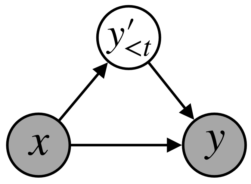
(a) AT

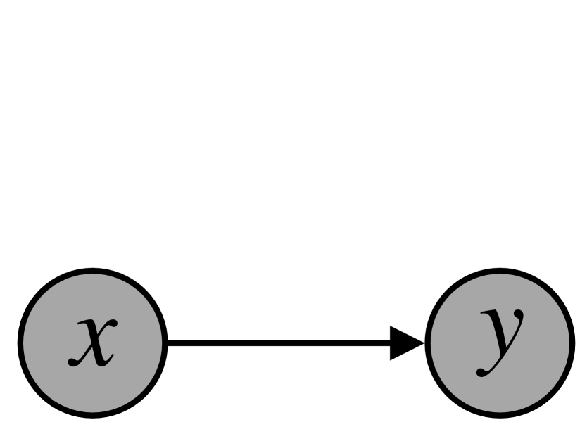
(b) NAT

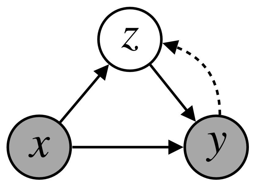
(c) LT

Figure 1: Different inference process of different Transformer models.

2.2 Latent Transformer

To bridge the gap between non-autoregressive and autoregressive decoding, Kaiser et al. (2018) introduce the Latent Transformer (LT). It incorporates non-autoregressive decoding with conditional dependency as the latent variable to alleviate the degradation resulted from the absence of dependency:

$$p(\bm{y}|\bm{x})=p(\bm{z}|\bm{x};\phi)\prod_{t=1}^{m}p(y_{t}|\bm{z},\bm{x};\theta),$$ (4)

where $\bm{z}=\{z_{1},\cdots,z_{L}\}$ is the latent sequence and the $L$ is the length of the latent sequence, $\phi$ and $\theta$ are the parameter of latent predictor and translation model, respectively.

The LT architecture stays unchanged from the origin NAT models, except for the latent predictor and decoder inputs. During inference, the Latent Transformer first autoregressively predicts the latent variables $\bm{z}$, then non-autoregressively produces the entire target sentence $\bm{y}$ conditioned on the latent sequence $\bm{z}$ (see Figure 1). Ma et al. (2019); Shu et al. (2019) extend this idea and model $\bm{z}$ as the continuous latent variables, achieving a promising result, which replaces the autoregressive predictor with the iterative transformation layer.

3 Approach

In this section, we present our proposed CNAT, an extension to the Transformer incorporated with non-autoregressive decoding for target tokens and autoregressive decoding for latent sequences.

In brief, CNAT follows the architecture of Latent Transformer Kaiser et al. (2018), except for the latent variable modeling (in $\S$ 3.1 and $\S$ 3.2) and inputs initialization (in $\S$ 3.3).

3.1 Modeling Target Categorical Information by Vector Quantization

Categorical information has achieved great success in neural machine translation, such as part-of-speech (POS) tag in autoregressive translation Yang et al. (2019) and syntactic label in non-autoregressive translation Akoury et al. (2019).

Inspired by the broad application of categorical information, we propose to model the implicit categorical information of target words in a non-autoregressive Transformer. Each target sequence $\bm{y}=y_{1:m}$ will be assigned to a discrete latent variable sequence $\bm{z}=z_{1:m}$. We assume that each $z_{i}$ will capture the fuzzy category of its token $y_{i}$. Then, the conditional probability $p(\bm{y}|\bm{x})$ is factorized with respect to the categorical latent variable:

$$p(\bm{y}|\bm{x})=\sum_{\bm{z}}p(\bm{z}|\bm{x})\cdot p(\bm{y}|\bm{z},\bm{x}).$$ (5)

However, it is computationally intractable to sum all configurations of latent variables. Following the spirit of the latent based model Kaiser et al. (2018); Roy et al. (2018), we employ a vector quantized technique to maintain differentiability through the categorical modeling and learn the latent variables straightforward.

Vector Quantization.

The vector quantization based methods have a long history of being successfully in machine learning models. In vector quantization, each target representation $\operatorname{repr}(y_{i})\in\mathbb{R}^{d_{\text{model}}}$ is passed through a discretization bottleneck using a nearest-neighbor lookup on embedding matrix $\mathbf{Q}\in\mathbb{R}^{K\times d_{\text{model}}}$, where $K$ is the number of categorical codes.

For each $y_{i}$ in the target sequence, we define its categorical variable $z_{i}$ and latent code $q_{i}$ as:

$$\begin{split}z_{i}&=k,\ q_{i}=\mathbf{Q}_{k},\\ \text{and}\ k&=\operatorname*{arg\,min}_{j\in[K]}||\operatorname{repr}(y_{i})-\mathbf{Q}_{j}||_{2},\end{split}$$ (6)

where $||\cdot||_{2}$ is the ${l}_{2}$ distance, $[K]$ denote the set $\{1,2,\cdots,K\}$. Intuitively, we adopt the embedding of $\bm{y}$ as the target representation:

$$\operatorname{repr}(y_{i})=\operatorname{embedding}(y_{i})$$

where the embedding matrix of the target language is shared with the $\operatorname{softmax}$ layer of the decoder.

Exponential Moving Average.

Following the common practice of vector quantization, we also employ the exponential moving average (EMA) technique to regularize the categorical codes.

Put simply, the EMA technique could be understood as basically the k-means clustering of the hidden states with a sort of momentum. We maintain an EMA over the following two quantities for each $j\in[K]$: 1) the count $c_{j}$ measuring the number of target representations that have $\mathbf{Q}_{j}$ as its nearest neighbor, and 2) $\mathbf{Q}_{j}$. The counts are updated over a mini-batch of targets $\{y_{1},y_{2},\cdots,y_{m\times B}\}$ with:

$$c_{j}=\lambda c_{j}+(1-\lambda)\sum_{i}^{m\times B}\operatorname{1}[z_{i}=j],$$ (7)

then, the latent code $\mathbf{Q}_{j}$ being updated with:

$$\mathbf{Q}_{j}=\lambda\mathbf{Q}_{j}+(1-\lambda)\sum_{i}^{m\times B}\frac{\operatorname{1}[z_{i}=j]\operatorname{repr}(y_{i})}{c_{j}},$$ (8)

where $\operatorname{1}[\cdot]$ is the indicator function and $\lambda$ is a decay parameter, $B$ is the size of the batch.

3.2 Modeling Categorical Sequence with Conditional Random Fields

Our next insight is transferring the dependencies among the target outputs into the latent spaces. Since the categorical variable captures the fuzzy target class information, it can be a proxy of the target outputs. We further employ a structural prediction module instead of the standard autoregressive Transformer to model the latent sequence. The former can explicitly model the dependencies among the latent variables and performs exact decoding during inference.

Conditional Random Fields.

We employ a linear-chain conditional random fields (CRF, Lafferty et al., 2001) to model the categorical latent variables, which is the most common structural prediction model.

Given the source input $\bm{x}=(x_{1},\cdots,x_{n})$ and its corresponding latent variable sequence $\bm{z}=(z_{1},\cdots,z_{m})$, the CRF model defines the probability of $\bm{z}$ as:

$$\begin{split}p(\bm{z}|\bm{x})=\frac{1}{\mathbb{Z}(\bm{x})}&\operatorname{exp}\Big{(}\sum_{i=1}^{m}s(z_{i},\bm{x},i)\\ &+\sum_{i=2}^{m}t(z_{i-1},z_{i},\bm{x},i)\Big{)},\end{split}$$ (9)

where $\mathbb{Z}(\bm{x})$ is the normalize factor, $s(z_{i},\bm{x},i)$ is the emit score of $z_{i}$ at the position $i$, and the $t(z_{i-1},z_{i},\bm{x},i)$ is the transition score from $z_{i-1}$ to $z_{i}$.

Before computing the emit score and transition score in Eq. 9, we first take $\bm{h}=h_{1:m}$ as the inputs and compute the representation $\bm{f}=\operatorname{Transfer}(\bm{h})$, where $\operatorname{Transfer}(\cdot)$ denotes a two-layer vanilla Transformer decoding function including a self-attention block, an encoder-decoder block followed by a feed-forward neural network block Vaswani et al. (2017).

We then compute the emit score and the transition score. For each position $i$, we compute the emit score with a linear transformation: $s(z_{i},\bm{x},i)=(W^{T}f_{i}+b)_{z_{i}}$ where $W\in\mathbb{R}^{d_{\text{model}}\times K}$ and $b\in\mathbb{R}^{K}$ are the parameters. We incorporate the positional context and compute its transition score with:

$$\begin{split}&\bm{M}_{\text{d}}^{i}=\operatorname{Biaffine}([f_{i-1};f_{i}]),\\ &\bm{M}^{i}=\bm{E}_{1}^{T}\bm{M}_{\text{d}}^{i}\bm{E}_{2},\\ &t(z_{i-1},z_{i},\bm{x},i)=\bm{M}_{z_{i-1},z_{i}}^{i},\end{split}$$ (10)

where $\operatorname{Biaffine}(\cdot):\mathbb{R}^{2d_{\text{model}}}\to\mathbb{R}^{d_{\text{t}}\times d_{\text{t}}}$ is a biaffine neural network Dozat and Manning (2017), $\bm{E}_{1}$ and $\bm{E}_{2}\in\mathbb{R}^{d_{\text{t}}\times K}$ are the transition matrix.

3.3 Fusing Source Inputs and Latent Codes via Gated Function

One potential issue is that the mismatch of the training and inference stage for the used categorical variables. Suppose we train the decoder with the quantized categorical variables $\bm{z}$, which is inferred from the target reference. In that case, we may fail to achieve satisfactory performance with the predicted categorical variables during inference.

We intuitively apply the gated neural network (denote as GateNet) to form the decoder inputs by fusing the copied decoder inputs $\bm{h}=h_{1:m}$ and the latent codes $\bm{q}=q_{1:m}$, since the copied decoder inputs $\bm{h}$ is still informative to non-autoregressive decoding:

$$\begin{split}g_{i}&=\sigma(\operatorname{FFN}([h_{i};q_{i}])),\\ o_{i}&=h_{i}*g_{i}+q(z_{i})*(1-g_{i}),\end{split}$$ (11)

where the $\operatorname{FFN}(\cdot):\mathbb{R}^{2d_{\text{model}}}\to\mathbb{R}^{d_{\text{model}}}$ is a two-layer feed-forward neural networks and $\sigma(.)$ is the $\operatorname{sigmoid}$ function.

3.4 Training

While training, we first compute the reference $\bm{z}^{\text{ref}}$ by the vector quantization and employ the EMA to update the quantized codes. The loss of the CRF-based predictor is computed with:

$$\mathcal{L}_{\text{crf}}=-\operatorname{log}p(\bm{z}^{\text{ref}}|\bm{x}).$$ (12)

To equip with the GateNet, we randomly mix the $\bm{z}^{\text{ref}}$ and the predicted $\bm{z}^{\text{pred}}$ as:

$$\bm{z}_{i}^{\text{mix}}=\left\{\begin{aligned} \bm{z}_{i}^{\text{pred}}&\quad\text{if}\ p\geq\tau\\ \bm{z}_{i}^{\text{ref\ \ \ }}&\quad\text{if}\ p<\tau\end{aligned}\right.,$$ (13)

where $p\sim\mathbb{U}[0,1]$ and $\tau$ is the threshold we set 0.5 in our experiments. Grounding on the $\bm{z}_{\text{mix}}$, the non-autoregressive translation loss is computed with:

$$\mathcal{L}_{\text{NAT}}=-\operatorname{log}p(\bm{y}|\bm{z}^{\text{mix}},\bm{x};\theta).$$ (14)

With the hyper-parameter $\alpha$, the overall training loss is:

$$\mathcal{L}=\mathcal{L}_{\text{NAT}}+\alpha\mathcal{L}_{\text{crf}}.$$ (15)

3.5 Inference

CNAT selects the best sequence by choosing the highest-probability latent sequence $z$ with Viterbi decoding Viterbi (1967), then generate the tokens with:

$$\bm{z}^{*} =\operatorname*{arg\,max}_{\bm{z}}p(\bm{z}|\bm{x};\theta),$$

$$\text{and}\ \bm{y}^{*} =\operatorname*{arg\,max}_{\bm{y}}p(\bm{y}|\bm{z}^{*},\bm{x};\theta),$$

where identifying $\bm{y}^{*}$ only requires independently maximizing the local probability for each output position.

4 Experiments

Datasets.

We conduct the experiments on the most widely used machine translation benchmarks: WMT14 English-German (WMT14 EN-DE, 4.5M pairs) and IWSLT14 German-English (IWSLT14, 160K pairs). The datasets are processed with the Moses script (Koehn et al., 2007), and the words are segmented into subword units using byte-pair encoding (Sennrich et al., 2016, BPE). We use the shared subword embeddings between the source language and target language for the WMT datasets and the separated subword embeddings for the IWSLT14 dataset.

Model Setting.

In the case of IWSLT14 task, we use a small setting ($d_{\text{model}}$ = 256, $d_{\text{hidden}}$ = 512, $p_{\text{dropout}}$ = 0.1, $n_{\text{layer}}$ = 5 and $n_{\text{head}}$ = 4) for Transformer and NAT models. For the WMT tasks, we use the Transformer-base setting ($d_{\text{model}}$ = 512, $d_{\text{hidden}}$ = 512, $p_{\text{dropout}}$ = 0.3, $n_{\text{head}}$ = 8 and $n_{\text{layer}}$ = 6) of the Vaswani et al. (2017). We set the hyperparameter $\alpha$ used in Eq. 15 and $\lambda$ in Eq. 7-8 to 1.0 and 0.999, respectively. The categorical number $K$ is set to 64 in our experiments. We implement our model based on the open-source framework of fairseq Ott et al. (2019).

Optimization.

We optimize the parameter with the Adam (Kingma and Ba, 2015) with $\beta=(0.9,0.98)$. We use inverse square root learning rate scheduling (Vaswani et al., 2017) for the WMT tasks and linear annealing schedule Lee et al. (2018) from $3\times 10^{-4}$ to $1\times 10^{-5}$ for the IWSLT14 task. Each mini-batch consists of 2048 tokens for IWSLT14 and 32K tokens for WMT tasks.

Distillation.

Sequence-level knowledge distillation (Hinton et al., 2015) is applied to alleviate the multi-modality problem Gu et al. (2018) while training. We follow previous studies on NAT (Gu et al., 2018; Lee et al., 2018; Wei et al., 2019) and use translations produced by a pre-trained autoregressive Transformer Vaswani et al. (2017) as the training data.

Reranking.

We also include the results that come at reranked parallel decoding (Gu et al., 2018; Guo et al., 2019; Wang et al., 2019; Wei et al., 2019), which generates several decoding candidates in parallel and selects the best via re-scoring using a pre-trained autoregressive model. Specifically, we first predict the target length $\hat{m}$ and generate output sequence with $\arg\max$ decoding for each length candidate $m\in[\hat{m}-\Delta m,\hat{m}+\Delta m]$ ($\Delta m$ = 4 in our experiments, means there are $N=9$ candidates), which was called length parallel decoding (LPD). Then, we use the pre-trained teacher to rank these sequences and identify the best overall output as the final output.

Baselines.

We compare the CNAT with several strong NAT baselines, including:

• The NAT builds upon latent variables: NAT-FT Gu et al. (2018), LT Kaiser et al. (2018), Syn-ST Akoury et al. (2019), LV-NAR Shu et al. (2019) and Flowseq Ma et al. (2019).

• The NAT with extra autoregressive decoding or iterative refinement: NAT-DCRF Sun et al. (2019), IR-NAT Lee et al. (2018), and CMLM Ghazvininejad et al. (2019).

• The NAT with auxiliary training objectives: NAT-REG Wang et al. (2019), imitate-NAT Wei et al. (2019).

We compare the proposed CNAT against baselines both in terms of generating quality and inference speedup. For all our tasks, we obtain the performance of baselines by either directly using the performance figures reported in the previous works if they are available or producing them by using the open-source implementation of baseline algorithms on our datasets.

Metrics.

We evaluate using the tokenized and cased BLEU scores (Papineni et al., 2002). We highlight the best NAT result with bold text.

4.1 Results

Model	WMT14		IWSLT14
	EN-DE	DE-EN	DE-EN
LV-NAR	11.80	/	/
AXE CMLM	20.40	24.90	/
SynST	20.74	25.50	23.82
Flowseq	20.85	25.40	24.75
NAT (ours)	9.80	11.02	17.77
CNAT (ours)	21.30	25.73	29.81

Table 1: Results of the NAT models with argmax decoding on test set of WMT14 and IWSLT14.

Translation Quality.

First, we compare CNAT with the NAT models without using advanced techniques, such as knowledge distillation, reranking, or iterative refinements. The results are listed in Table 1. The CNAT achieves significant improvements (around 11.5 BLEU in EN-DE, more than 14.5 BLEU in DE-EN) over the vanilla NAT, which indicates that modeling categorical information could improve the modeling capability of the NAT model. Also, the CNAT achieves better results than Flowseq and SynST, which demonstrates the effectiveness of CNAT in modeling dependencies between the target outputs.

Model	WMT14		IWSLT14
	EN-DE	DE-EN	DE-EN
NAT-FT	17.69	21.47	/
LT	19.80	/	/
NAT-REG	20.65	24.77	23.89
imitate-NAT	22.44	25.67	/
Flowseq	23.72	28.39	27.55
NAT-DCRF	23.44	27.22	27.44
Transformer (ours)	27.33	31.69	34.29
NAT (ours)	17.69	18.93	23.78
CNAT (ours)	25.56	29.36	31.15

Table 2: Results of NAT models trained with knowledge distillation on test set of WMT14 and IWSLT14.

The performance of the NAT models with advance techniques (sequence-level knowledge distillation or reranking) is listed in Table 2 and Table 3. Coupling with the knowledge distillation techniques, all NAT models achieve remarkable improvements.

Model	N	WMT14
		EN-DE	DE-EN
NAT-FT	10	18.66	22.42
NAT-FT	100	19.17	23.20
LT	10	21.00	/
LT	100	22.50	/
NAT-REG	9	24.61	28.90
imitate-NAT	9	24.15	27.28
Flowseq	15	24.70	29.44
Flowseq	30	25.31	30.68
NAT-DCRF	9	26.07	29.68
NAT-DCRF	19	26.80	30.04
Transformer (ours)	-	27.33	31.69
CNAT (ours)	9	26.60	30.75

Table 3: Results of NAT models with parallel decoding on test set of WMT14. “N” means the number of candidates to be re-ranked.

Our best results are obtained with length parallel decoding, which employs a pretrained Transformer to rerank the multiple parallels generated candidates of different target lengths. Specifically, on a large scale WMT14 dataset, CNAT surpasses the NAT-DCRF by 0.71 BLEU score in DE-EN but slightly under the NAT-DCRF around 0.20 BLEU in EN-DE, which shows that the CNAT is comparable to the state-of-the-art NAT model. Also, we can see that a larger “N” leads to better results ($N=100$ vs. $N=10$ of NAT-FT, $N=19$ vs. $N=9$ of NAT-DCRF, etc.); however, it always comes at the degradation of decoding efficiency.

Model	Iteration	WMT14
		EN-DE	DE-EN	Speedup
IR-NAT	1	13.91	16.77	11.39$\times$
	2	16.95	20.39	8.77$\times$
	5	20.26	23.86	3.11$\times$
	10	21.61	25.48	2.01$\times$
CMLM	4	26.08	30.11	/
	10	26.92	30.86	/
CNAT	1	25.56	29.36	10.37$\times$
CNAT (N=9)	1	26.60	30.75	5.59$\times$

Table 4: Results of NAT models with iterative refinements on test set of WMT14. “Iteration” means the number of iteration refinements.

We also compare our CNAT with the NAT models that employ an iterative decoding technique and list the results in Table 4. The iterative-based non-autoregressive Transformer captures the target language’s dependencies by iterative generating based on the previous iteration output, which is an important exploration for a non-autoregressive generation. With the iteration number increasing, the performance improving, the decoding speed-up dropping, whatever the IR-NAT or CMLM. We can see that the CNAT achieves a better result than the CMLM with four iterations and IR-NAT with ten iterations, even close to the CMLM with ten iterations while keeping the benefits of a one-shot generation.

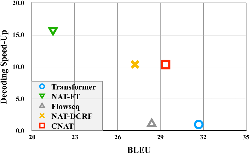
(a) Pure NAT decoding.

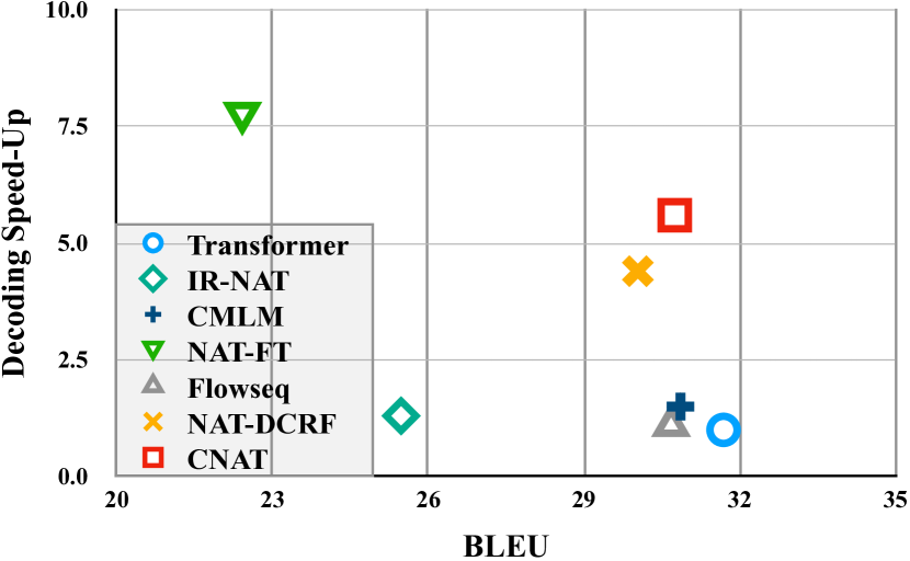
(b) NAT with advanced decoding techniques.

Figure 2: BLEU and decoding speed-up of NAT models on WMT14 DE-EN test set. Each point represents the decoding method run with its corresponding setting in Table 2, Table 3 or Table 4.

Translation Efficiency.

As depicted in Figure 2, we validate the efficiency of CNAT. Put simply, the decoding speed is measured sentence-by-sentence, and the speed-up is computed by comparing it with the Transformer. Figure 2(a) and Figure 2(b) show the BLEU scores and decoding speed-up of NAT models. The former compares the pure NAT models. The latter compares NAT model inference with advanced decoding techniques (parallel reranking or iterative-based decoding).

We can see from Figure 2 that the point of CNAT is located on the top-right of the baselines. The CNAT outperforms our baselines in BLEU if speed-up is held, and in speed-up if BLEU is held, indicating CNAT outperforms previous state-of-the-art NAT methods. Although iterative models like CMLM achieves competitive BLEU scores, they only maintain minor speed advantages over Transformer. In contrast, CNAT remarkably improves the inference speed while keeping a competitive performance.

Methods	Latent BLEU	Translation BLEU
CNAT w/ $\bm{z}_{\text{ref}}$	100.00	59.12
CNAT w/ $m_{\text{ref}}$	39.72	31.59
CNAT	38.59	31.15

Table 5: Results on the test of IWSLT14 to analyze the effectiveness of categorical modeling. “w/ $\bm{z}_{\text{ref}}$” denote CNAT generate the tokens condition on the latent sequence which is quantized from the reference target. “w/ $m_{\text{ref}}$” denote the CNAT generate the tokens condition on the reference length.

Effectiveness of Categorical Modeling.

We further conduct the experiments on the test set of IWSLT14 to analyze the effectiveness of our categorical modeling and its influence on translation quality. We regard the categorical predictor as a sequence-level generation task and list its BLEU score in Table 5.

As see, a better latent prediction can yield a better translation. With the $\bm{z}_{\text{ref}}$ as the latent sequence, the model achieves surprisingly good performance on this task, showing the usefulness of the learned categorical codes. We also can see that the CNAT decoding with reference length only slightly  (0.44 BLEU) better than it with predicted length, indicating that the model is robust.

Line	$K$				Predictor		GateNet	BLEU
	32	64	128		CRF	AR
1	✓				✓		✓	30.13
2		✓			✓		✓	31.87
3			✓		✓		✓	30.82
4		✓			✓			29.32
5		✓				✓	✓	28.23
6		✓				✓		24.00
7			✓			✓		25.43
8								24.25

Table 6: Ablation study on the dev set of IWSLT14. Note that we train all of the configurations with knowledge distillation. “AR” denotes an autoregressive Transformer predictor. The line 8 is our NAT baseline.

4.2 Ablation Study

We further conduct the ablation study with different CNAT variant on dev set of IWSLT14.

Influence of $K$.

We can see the CRF with the categorical number $K=64$ achieves the highest score (line 2). A smaller or larger $K$ neither has a better result. The AR predictor may have a different tendency: with a larger $K=128$, it achieves a better performance. However, a larger $K$ may lead to a higher latency while inference, which is not the best for non-autoregressive decoding. In our experiments, the $K=64$ can achieve the high-performance and be smaller enough to keep the low-latency during inference.

CRF versus AR.

Experiment results show that the CRF-based predictor is better than the AR predictor. We can see that the CRF-based predictor surpasses the Transformer predictor 3.5 BLEU (line 2 vs. line 5) with the GateNet; without the GateNet, the gap enlarges to 5.3 BLEU (line 4 vs. line 6). It is consistent with our intuition that CRF is better than Transformer to model the dependencies among latent variables on machine translation when the number of categories is small.

GateNet.

Without the GateNet, the CNAT with AR predictor degenerates a standard LT model with a smaller latent space. We can see its performance is even lower than the NAT-baselines (line 6 vs. line 8). Equipping with the GateNet and the schedule sampling, it outperforms the NAT baseline with a large margin (around 4.0 BLEU), showing that the GateNet mechanism plays an essential role in our proposed model.

4.3 Code Study

To analyze the learned category, we further compute its relation to two off-the-shelf categorical information: the part-of-speech (POS) tags and the frequency-based clustered classes. For the former, we intuitively assign the POS tag of a word to its sub-words and compute the POS tag frequency for the latent codes. For the latter, we roughly assign the category of a subword according to its frequency. It needs to mention that the number of frequency-based classes is the same as that of the POS tags.

	H-score	C-score	V-measure
w/ POS tags	0.70	0.47	0.56
w/ Frequency	0.62	0.48	0.54

Table 7: Clustering evaluation metrics on the test set of IWSLT14 to analyze the learned codes.

Quantitative Results.

We first compute the V-Measure Rosenberg and Hirschberg (2007) score between the latent categories to POS tags and sub-words frequencies. The results are listed in Table 7.

Overall, the “w/ POS tags” achieves a higher V-Measure score, indicating that the latent codes are more related to the POS tags than sub-words frequencies. The homogeneity score (H-score) evaluates the purity of the category. We also can see that the former has a relatively higher H-score than the latter (0.70 vs. 0.62), which is consistent with our intuition.

Figure 3: The POS tags distribution for the top 10 frequent latent variables on the test set of IWSLT14. We list the top 3 frequent POS tags for each latent variable.

Case Analysis.

As shown in Figure 3, we also depict the POS tags distribution for the top 10 frequent latent variables on the test set of IWSLT14. We can see a sharp distribution for each latent variable, showing that our learned fuzzy classes are meaningful.

5 Related Work

Non-autoregressive Machine Translation.

Gu et al. (2018) first develop a non-autoregressive Transformer (NAT) for machine translation, which produces the outputs in parallel, and the inference speed is thus significantly boosted. Due to the missing of dependencies among the target outputs, the translation quality is largely sacrificed.

A line of work proposes to mitigate such performance degradation by enhancing the decoder inputs. Lee et al. (2018) propose a method of iterative refinement based on the previous outputs. Guo et al. (2019) enhance decoder input by introducing the phrase table in statistical machine translation and embedding transformation. There are also some work focuses on improving the decoder inputs’ supervision, including imitation learning from autoregressive models (Wei et al., 2019) or regularizing the hidden state with backward reconstruction error (Wang et al., 2019).

Another work proposes modeling the dependencies among target outputs, which is explicitly missed in the vanilla NAT models. Qian et al. (2020); Ghazvininejad et al. (2019) propose to model the target-side dependencies with a masked language model, modeling the directed dependencies between the observed target and the unobserved words. Different from their work, we model the target-side dependencies in the latent space, which follows the latent variable Transformer fashion.

Latent Variable Transformer.

More close to our work is the latent variable Transformer, which takes the latent variable as inputs to modeling the target-side information. Shu et al. (2019) combine continuous latent variables and deterministic inference procedure to find the target sequence that maximizes the lower bound to the log-probability. Ma et al. (2019) propose to use generative flows to the model complex prior distribution. Kaiser et al. (2018) propose to autoregressively decode a shorter latent sequence encoded from the target sentence, then simultaneously generate the sentence from the latent sequence. Bao et al. (2019) model the target position of decode input as a latent variable and introduce a heuristic search algorithm to guide the position learning. Akoury et al. (2019) first autoregressively predict a chunked parse tree and then simultaneously generate the target tokens from the predicted syntax.

6 Conclusion

We propose CNAT, which implicitly models the categorical codes of the target language, narrowing the performance gap between the non-autoregressive decoding and autoregressive decoding. Specifically, CNAT builds upon the latent Transformer and models the target-side categorical information with vector quantization and conditional random fields (CRF) model. We further employ a gated neural network to form the decoder inputs. Equipped with the scheduled sampling, CNAT works more robust. As a result, the CNAT achieves a significant improvement and moves closer to the performance of the Transformer on machine translation.

Appendix A Non-Indo-European Translation

Dataset.

We apply the CNAT to the non-Indo-European translation tasks on the LDC Chinese-English (denote as LDC ZH-EN, 1.30M sentence pairs) and MT02 test set of NIST ZH-EN dataset. We use NLPIRICTCLAS and Moses tokenizer for Chinese and English tokenization, respectively.

Model	BLEU
Transformer	28.05
NAT	12.31
CNAT	22.16

Table 8: Results on the MT02 set of different models.

Results.

We can see than in Table 8 that our model can enhance the performance of NAT with a large margin (22.16 vs. 12.31).

Appendix B Learned Latent Codes

ID	Top 1	Top 2	Top 3
0	NOUN(41.06%)	ADJ(20.74%)	VERB(20.09%)
1	NOUN(88.73%)	ADJ(3.48%)	VERB(2.34%)
2	NOUN(58.06%)	ADJ(15.40%)	VERB(12.29%)
3	PUNCT(100.00%)	—	—
4	PUNCT(99.80%)	NOUN(0.14%)	PROPN(0.05%)
5	PRON(99.29%)	NOUN(0.42%)	PROPN(0.20%)
6	VERB(77.95%)	NOUN(9.93%)	ADJ(8.45%)
7	DET(99.33%)	PUNCT(0.47%)	PART(0.15%)
8	ADJ(56.24%)	ADV(15.06%)	NUM(11.87%)
9	NOUN(52.01%)	VERB(16.72%)	ADJ(15.75%)
10	CCONJ(99.71%)	VERB(0.11%)	NOUN(0.11%)
11	PART(71.00%)	ADP(27.70%)	SCONJ(0.99%)
12	PRON(60.71%)	SCONJ(30.15%)	DET(8.88%)
13	ADP(90.70%)	SCONJ(5.91%)	ADV(3.09%)
14	DET(96.81%)	NOUN(1.81%)	PROPN(1.13%)
15	NOUN(88.49%)	VERB(4.28%)	ADV(3.10%)
16	VERB(90.35%)	NOUN(4.82%)	AUX(4.40%)
17	ADV(67.37%)	PART(15.02%)	NOUN(8.31%)
18	PRON(68.46%)	DET(29.31%)	NOUN(1.65%)
19	ADV(61.05%)	SCONJ(36.01%)	ADP(2.31%)
20	VERB(93.70%)	NOUN(6.03%)	PROPN(0.23%)
21	PRON(98.59%)	NOUN(0.78%)	ADJ(0.39%)
22	ADP(93.45%)	ADV(2.40%)	SCONJ(1.95%)
23	AUX(85.14%)	VERB(14.51%)	NOUN(0.36%)
24	AUX(80.60%)	VERB(18.55%)	NOUN(0.60%)
25	VERB(44.78%)	AUX(40.84%)	PROPN(13.49%)
26	ADP(73.68%)	ADV(9.68%)	SCONJ(9.55%)
27	AUX(99.47%)	NOUN(0.53%)	—
28	AUX(76.11%)	VERB(10.26%)	PART(9.70%)
29	ADP(89.48%)	ADV(3.93%)	NOUN(3.93%)
30	VERB(43.34%)	ADP(34.41%)	AUX(14.47%)
31	DET(53.56%)	PRON(46.44%)	—
32	ADV(95.89%)	SCONJ(3.72%)	PROPN(0.23%)
33	ADP(52.12%)	SCONJ(27.84%)	ADV(8.74%)
34	DET(62.63%)	PRON(20.73%)	ADV(9.90%)
35	VERB(76.34%)	AUX(23.66%)	—
36	AUX(100.00%)	—	—
37	ADV(47.90%)	PRON(40.51%)	NOUN(11.59%)
38	NOUN(99.17%)	ADJ(0.73%)	ADV(0.10%)
39	NOUN(35.74%)	VERB(28.94%)	ADJ(28.21%)
40	NOUN(49.84%)	ADJ(27.23%)	ADV(16.19%)
41	PRON(92.22%)	NOUN(4.75%)	PROPN(1.08%)
42	PRON(92.73%)	DET(7.05%)	ADV(0.22%)
43	ADP(32.17%)	NOUN(23.05%)	ADJ(21.61%)
44	PUNCT(100.00%)	—	—
45	PRON(100.00%)	—	—
46	AUX(94.36%)	VERB(4.59%)	NOUN(1.05%)
47	ADV(67.33%)	ADJ(31.75%)	NOUN(0.79%)
48	ADP(91.70%)	SCONJ(8.16%)	ADJ(0.14%)
49	PUNCT(100.00%)	—	—
50	PART(70.91%)	AUX(25.04%)	ADP(2.85%)
51	CCONJ(99.52%)	ADP(0.48%)	—
52	ADP(69.34%)	SCONJ(15.89%)	ADV(14.13%)
53	PUNCT(100.00%)	—	—
54	NOUN(58.00%)	VERB(30.58%)	ADJ(6.15%)
55	VERB(71.57%)	AUX(28.04%)	NOUN(0.39%)
56	NUM(75.73%)	NOUN(20.33%)	PRON(2.49%)
57	DET(86.03%)	ADJ(6.77%)	PROPN(3.71%)
58	ADP(61.07%)	ADV(31.77%)	NOUN(5.37%)
59	CCONJ(90.75%)	NOUN(8.48%)	ADJ(0.51%)
60	ADP(78.74%)	SCONJ(19.93%)	ADV(1.00%)
61	VERB(59.11%)	NOUN(31.56%)	ADJ(9.33%)

Table 9: The distribution of pos tags for latent variables. For each latent variable, we list the top 3 frequent pos tags and their corresponding percentages.

References

- Akoury et al. (2019) Nader Akoury, Kalpesh Krishna, and Mohit Iyyer. 2019. Syntactically supervised transformers for faster neural machine translation. In Proceedings of the 57th Annual Meeting of the Association for Computational Linguistics, pages 1269–1281, Florence, Italy. Association for Computational Linguistics.
- Bao et al. (2019) Yu Bao, Hao Zhou, Jiangtao Feng, Mingxuan Wang, Shujian Huang, Jiajun Chen, and Lei Li. 2019. Non-autoregressive transformer by position learning. arXiv preprint arXiv:1911.10677.
- Bengio et al. (2015) Samy Bengio, Oriol Vinyals, Navdeep Jaitly, and Noam Shazeer. 2015. Scheduled sampling for sequence prediction with recurrent neural networks. In Advances in Neural Information Processing Systems 28: Annual Conference on Neural Information Processing Systems 2015, December 7-12, 2015, Montreal, Quebec, Canada, pages 1171–1179.
- Dozat and Manning (2017) Timothy Dozat and Christopher D. Manning. 2017. Deep biaffine attention for neural dependency parsing. In 5th International Conference on Learning Representations, ICLR 2017, Toulon, France, April 24-26, 2017, Conference Track Proceedings. OpenReview.net.
- Ghazvininejad et al. (2019) Marjan Ghazvininejad, Omer Levy, Yinhan Liu, and Luke Zettlemoyer. 2019. Mask-predict: Parallel decoding of conditional masked language models. In Proceedings of the 2019 Conference on Empirical Methods in Natural Language Processing and the 9th International Joint Conference on Natural Language Processing (EMNLP-IJCNLP), pages 6112–6121, Hong Kong, China. Association for Computational Linguistics.
- Gu et al. (2018) Jiatao Gu, James Bradbury, Caiming Xiong, Victor O. K. Li, and Richard Socher. 2018. Non-autoregressive neural machine translation. In 6th International Conference on Learning Representations, ICLR 2018, Vancouver, BC, Canada, April 30 - May 3, 2018, Conference Track Proceedings. OpenReview.net.
- Guo et al. (2019) Junliang Guo, Xu Tan, Di He, Tao Qin, Linli Xu, and Tie-Yan Liu. 2019. Non-autoregressive neural machine translation with enhanced decoder input. In The Thirty-Third AAAI Conference on Artificial Intelligence, AAAI 2019, The Thirty-First Innovative Applications of Artificial Intelligence Conference, IAAI 2019, The Ninth AAAI Symposium on Educational Advances in Artificial Intelligence, EAAI 2019, Honolulu, Hawaii, USA, January 27 - February 1, 2019, pages 3723–3730. AAAI Press.
- Hinton et al. (2015) Geoffrey Hinton, Oriol Vinyals, and Jeff Dean. 2015. Distilling the knowledge in a neural network. arXiv preprint arXiv:1503.02531.
- Kaiser et al. (2018) Lukasz Kaiser, Samy Bengio, Aurko Roy, Ashish Vaswani, Niki Parmar, Jakob Uszkoreit, and Noam Shazeer. 2018. Fast decoding in sequence models using discrete latent variables. In Proceedings of the 35th International Conference on Machine Learning, ICML 2018, Stockholmsmässan, Stockholm, Sweden, July 10-15, 2018, volume 80 of Proceedings of Machine Learning Research, pages 2395–2404. PMLR.
- Kingma and Ba (2015) Diederik P. Kingma and Jimmy Ba. 2015. Adam: A method for stochastic optimization. In 3rd International Conference on Learning Representations, ICLR 2015, San Diego, CA, USA, May 7-9, 2015, Conference Track Proceedings.
- Koehn et al. (2007) Philipp Koehn, Hieu Hoang, Alexandra Birch, Chris Callison-Burch, Marcello Federico, Nicola Bertoldi, Brooke Cowan, Wade Shen, Christine Moran, Richard Zens, Chris Dyer, Ondřej Bojar, Alexandra Constantin, and Evan Herbst. 2007. Moses: Open source toolkit for statistical machine translation. In Proceedings of the 45th Annual Meeting of the Association for Computational Linguistics Companion Volume Proceedings of the Demo and Poster Sessions, pages 177–180, Prague, Czech Republic. Association for Computational Linguistics.
- Lafferty et al. (2001) John D. Lafferty, Andrew McCallum, and Fernando C. N. Pereira. 2001. Conditional random fields: Probabilistic models for segmenting and labeling sequence data. In Proceedings of the Eighteenth International Conference on Machine Learning (ICML 2001), Williams College, Williamstown, MA, USA, June 28 - July 1, 2001, pages 282–289. Morgan Kaufmann.
- Lee et al. (2018) Jason Lee, Elman Mansimov, and Kyunghyun Cho. 2018. Deterministic non-autoregressive neural sequence modeling by iterative refinement. In Proceedings of the 2018 Conference on Empirical Methods in Natural Language Processing, pages 1173–1182, Brussels, Belgium. Association for Computational Linguistics.
- Li et al. (2019) Zhuohan Li, Di He, Fei Tian, Tao Qin, Liwei Wang, and Tie-Yan Liu. 2019. Hint-based training for non-autoregressive translation. In NeuralIPS (to appear).
- Ma et al. (2019) Xuezhe Ma, Chunting Zhou, Xian Li, Graham Neubig, and Eduard Hovy. 2019. FlowSeq: Non-autoregressive conditional sequence generation with generative flow. In Proceedings of the 2019 Conference on Empirical Methods in Natural Language Processing and the 9th International Joint Conference on Natural Language Processing (EMNLP-IJCNLP), pages 4282–4292, Hong Kong, China. Association for Computational Linguistics.
- Ott et al. (2019) Myle Ott, Sergey Edunov, Alexei Baevski, Angela Fan, Sam Gross, Nathan Ng, David Grangier, and Michael Auli. 2019. fairseq: A fast, extensible toolkit for sequence modeling. In Proceedings of the 2019 Conference of the North American Chapter of the Association for Computational Linguistics (Demonstrations), pages 48–53, Minneapolis, Minnesota. Association for Computational Linguistics.
- Papineni et al. (2002) Kishore Papineni, Salim Roukos, Todd Ward, and Wei-Jing Zhu. 2002. Bleu: a method for automatic evaluation of machine translation. In Proceedings of the 40th Annual Meeting of the Association for Computational Linguistics, pages 311–318, Philadelphia, Pennsylvania, USA. Association for Computational Linguistics.
- Qian et al. (2020) Lihua Qian, Hao Zhou, Yu Bao, Mingxuan Wang, Lin Qiu, Weinan Zhang, Yong Yu, and Lei Li. 2020. Glancing transformer for non-autoregressive neural machine translation. arXiv preprint arXiv:2008.07905.
- Rosenberg and Hirschberg (2007) Andrew Rosenberg and Julia Hirschberg. 2007. V-measure: A conditional entropy-based external cluster evaluation measure. In Proceedings of the 2007 Joint Conference on Empirical Methods in Natural Language Processing and Computational Natural Language Learning (EMNLP-CoNLL), pages 410–420, Prague, Czech Republic. Association for Computational Linguistics.
- Roy et al. (2018) Aurko Roy, Ashish Vaswani, Niki Parmar, and Arvind Neelakantan. 2018. Towards a better understanding of vector quantized autoencoders. arXiv.
- Sennrich et al. (2016) Rico Sennrich, Barry Haddow, and Alexandra Birch. 2016. Neural machine translation of rare words with subword units. In Proceedings of the 54th Annual Meeting of the Association for Computational Linguistics (Volume 1: Long Papers), pages 1715–1725, Berlin, Germany. Association for Computational Linguistics.
- Shu et al. (2019) Raphael Shu, Jason Lee, Hideki Nakayama, and Kyunghyun Cho. 2019. Latent-variable non-autoregressive neural machine translation with deterministic inference using a delta posterior. arXiv preprint arXiv:1908.07181.
- Sun et al. (2019) Zhiqing Sun, Zhuohan Li, Haoqing Wang, Di He, Zi Lin, and Zhi-Hong Deng. 2019. Fast structured decoding for sequence models. In Advances in Neural Information Processing Systems 32: Annual Conference on Neural Information Processing Systems 2019, NeurIPS 2019, December 8-14, 2019, Vancouver, BC, Canada, pages 3011–3020.
- Vaswani et al. (2017) Ashish Vaswani, Noam Shazeer, Niki Parmar, Jakob Uszkoreit, Llion Jones, Aidan N. Gomez, Lukasz Kaiser, and Illia Polosukhin. 2017. Attention is all you need. In Advances in Neural Information Processing Systems 30: Annual Conference on Neural Information Processing Systems 2017, December 4-9, 2017, Long Beach, CA, USA, pages 5998–6008.
- Viterbi (1967) Andrew Viterbi. 1967. Error bounds for convolutional codes and an asymptotically optimum decoding algorithm. IEEE transactions on Information Theory, 13(2):260–269.
- Wang et al. (2019) Yiren Wang, Fei Tian, Di He, Tao Qin, ChengXiang Zhai, and Tie-Yan Liu. 2019. Non-autoregressive machine translation with auxiliary regularization. In AAAI.
- Wei et al. (2019) Bingzhen Wei, Mingxuan Wang, Hao Zhou, Junyang Lin, and Xu Sun. 2019. Imitation learning for non-autoregressive neural machine translation. In Proceedings of the 57th Annual Meeting of the Association for Computational Linguistics, pages 1304–1312, Florence, Italy. Association for Computational Linguistics.
- Yang et al. (2019) Xuewen Yang, Yingru Liu, Dongliang Xie, Xin Wang, and Niranjan Balasubramanian. 2019. Latent part-of-speech sequences for neural machine translation. In Proceedings of the 2019 Conference on Empirical Methods in Natural Language Processing and the 9th International Joint Conference on Natural Language Processing (EMNLP-IJCNLP), pages 780–790, Hong Kong, China. Association for Computational Linguistics.