A variational interpretation of Restricted Additive Schwarz with impedance transmission condition for the Helmholtz problem

Abstract

In this paper we revisit the Restricted Additive Schwarz method for solving discretized Helmholtz problems, using impedance boundary conditions on subdomains (sometimes called ORAS). We present this method in its variational form and show that it can be seen as a finite element discretization of a parallel overlapping domain decomposition method defined at the PDE level. In a recent companion paper, the authors have proved certain contractive properties of the error propagation operator for this method at the PDE level, under certain geometrical assumptions. We illustrate computationally that these properties are also enjoyed by its finite element approximation, i.e., the ORAS method.

1 The Helmholtz problem

Motivated by the large range of applications, there is currently great interest in designing and analysing preconditioners for finite element discretisations of the Helmholtz equation

$$-(\Delta+k^{2}\,)u\ =\ f\quad\text{on}\quad\Omega\,,$$ (1)

on a $d-$dimensional domain $\Omega$ ($d=2,3$), with $k$ the (assumed constant, but possibly large) angular frequency. While the methods presented easily apply to quite general scattering problems and geometries, we restrict attention here to the interior impedance problem, where $\Omega$ is bounded, and the boundary condition is

$$\left(\frac{\partial}{\partial n}-{\rm i}k\right)u=g\quad\text{on}\quad\partial\Omega\,,$$ (2)

where $\partial u/\partial n$ is the outward-pointing normal derivative of $u$ on $\Omega$.

The weak form of problem (1), (2) is to seek $u\in H^{1}(\Omega)$ such that

$$a(u,v)=F(v):=\int_{\Omega}f\bar{v}~{}dx+\int_{\partial\Omega}g\bar{v}~{}ds,$$ (3)

$$\text{where}\quad\quad a(u,v):=\int_{\Omega}(\nabla u.\nabla\overline{v}-k^{2}u\overline{v})-{\rm i}k\int_{\partial\Omega}u\overline{v},\quad\text{for}\quad u,v\in H^{1}(\Omega).$$

2 Parallel iterative Schwarz method

To solve (1), (2), we shall consider domain decomposition methods, based on a set of Lipschitz polyhedral subdomains $\{\Omega_{\ell}\}_{\ell=1}^{N}$, forming an overlapping cover of $\Omega$ and equipped with a partition of unity: $\{\chi_{\ell}\}_{\ell=1}^{N}$, such that

$$\left.\begin{array}[]{ll}\text{for each}\quad\ell:&\ \mathrm{supp}\chi_{\ell}\subset\overline{\Omega_{\ell}},\quad 0\leq\chi_{\ell}(\boldsymbol{x})\leq 1\,\,\text{when }\boldsymbol{x}\in\overline{\Omega_{\ell}},\\ &\\ \quad\text{ and }&\sum_{\ell}\chi_{\ell}(\boldsymbol{x})=1\,\text{ for all }\boldsymbol{x}\in\overline{\Omega}.\end{array}\right\}$$ (4)

Then, the parallel Schwarz method for (1), (2) with Robin (impedance) transmission conditions is: given $u^{n}$ defined on $\Omega$, we solve the local problems:

$$-(\Delta+k^{2})u_{\ell}^{n+1} =f\quad \text{in }\ \Omega_{\ell}\,,$$ (5)

$$\left(\frac{\partial}{\partial n_{\ell}}-{\rm i}k\right)u_{\ell}^{n+1} =\left(\frac{\partial}{\partial n_{\ell}}-{\rm i}k\right)u^{n}\quad \text{on }\ \partial\Omega_{\ell}\backslash\partial\Omega\,,$$ (6)

$$\left(\frac{\partial}{\partial n_{\ell}}-{\rm i}k\right)u_{\ell}^{n+1} =g\quad \text{on }\ \partial\Omega_{\ell}\cap\partial\Omega.$$ (7)

Then the next iterate is the weighted sum of the local solutions

$$u^{n+1}:=\sum_{\ell}\chi_{\ell}u_{\ell}^{n+1}.$$ (8)

Information is shared between neighbouring subdomains at each iteration via (8).

In GoGaGrLaSp:21 , we analyse the iteration (5) – (8) in the function space

$$U(\Omega):=\big{\{}v\in H^{1}(\Omega):\,\Delta v\in L^{2}(\Omega),\,\partial v/\partial n\in L^{2}(\partial\Omega)\big{\}},$$

and its local analogues $U(\Omega_{\ell})$. Using the fact that any function $v\in U(\Omega_{\ell})$ has impedance trace $(\partial/\partial n-{\rm i}k)v\in L^{2}(\Gamma)$ on any Lipschitz curve $\Gamma\subset\Omega_{\ell}$, we prove in GoGaGrLaSp:21 that (5) – (8) is well-defined in the space $U(\Omega)$. Moreover, introducing $e_{\ell}^{n}=u|_{\Omega_{\ell}}-u^{n}_{\ell}$, and letting $\mathbf{e}^{n}=(e_{1}^{n},\ldots,e_{N}^{n})$, we prove in GoGaGrLaSp:21 that $\mathbf{e}^{n+1}={\mathcal{T}}\mathbf{e}^{n},$ where under certain geometric assumptions, ${\mathcal{T}}$ has the ‘power contraction’ property

$$\|{\mathcal{T}}^{N}\|\ll 1,$$ (9)

with respect to the product norm on $\prod_{\ell}U_{0}(\Omega_{\ell})$, where $U_{0}(\Omega_{\ell})$ is the subspace of functions $v\in U(\Omega_{\ell})$, for which $\Delta v+k^{2}v=0$ on $\Omega_{\ell}$. Analogously to BeDe:97 , the norm of $v$ is the $L^{2}$ norm of its impedance data on $\partial\Omega_{\ell}$. See the remarks in §5, especially (24), for a more precise explanation of (9).

The aim of this note is to show that a natural finite element analogue of (5) – (8) corresponds to a preconditioned Richardson-type iterative method for the finite element approximation of (1), (2), where the preconditioner is a Helmholtz-orientated version of the popular Restricted Additive Schwarz method. This preconditioner is given several different names in the literature – WRAS-H (Weighted RAS for Helmholtz) KiSa:07 , ORAS (Optimized Restricted Additive Schwarz) st2007optimized ; DoJoNa:15 ; GoGrSp:20 , IMPRAS1 (RAS with impedance boundary condition) GrSpVa:17a . However it has not previously been directly connected via a variational argument to the iterative method (5) – (8) in the Helmholtz case, although there are algebraic discussions (e.g., EfGa:03 , (DoJoNa:15, , §2.3.2)). We also demonstrate numerically in §5, that the finite element analogue of (5) – (8) inherits the property (9) proved at the continuous level in GoGaGrLaSp:21 .

Method (5)–(8) is an example of methods studied more generally in the Optimized Schwarz literature (e.g., gander2006optimized ; st2007optimized ), where Robin (or more sophisticated) transmission conditions are constructed with the aim of optimizing convergence rates. Although the transmission condition (6) above can be justified directly as a first order absorbing condition for the local Helmholtz problem (5) (without considering optimization), this method is still often called ‘Optimized Restricted Additive Schwarz’ (or ‘ORAS’) and we shall continue this naming convention here. ORAS is arguably the most successful one-level parallel method for Helmholtz problems. It can be applied on very general geometries, does not depend on parameters, and can even be robust to increasing $k$ GoGrSp:20 . More generally it can be combined with coarse spaces to improve its robustness properties.

3 Variational formulation of RAS with impedance transmission condition (ORAS)

Here we formulate a finite element approximation of (1), (2) and show that it coincides with ORAS. We introduce a nodal finite element space ${\mathcal{V}}^{h}\subset H^{1}(\Omega)$ consisting of continuous piecewise polynomials of total degree $\leq p$ on a conforming mesh ${\mathcal{T}}^{h}$. Functions in ${\mathcal{V}}^{h}$ are uniquely determined by their values at nodes in $\overline{\Omega}$, denoted $\{x_{j}:j\in{\mathcal{I}}\}$, for some index set ${\mathcal{I}}$. The local space on $\overline{\Omega_{\ell}}$ is ${\mathcal{V}}_{\ell}^{h}:=\{v_{h}|_{\overline{\Omega_{\ell}}}~{}:~{}v_{h}\in{{\mathcal{V}}}^{h}\}$ with corresponding nodes denoted $\{x_{j}:j\in{\mathcal{I}}_{\ell}\}$, for some ${\mathcal{I}}_{\ell}\subset{\mathcal{I}}$.

Using the sesquilinear form $a$ and right-hand side $F$ appearing in (3), we can define the discrete operators ${\mathcal{A}}_{h},F_{h}:{\mathcal{V}}^{h}\mapsto({\mathcal{V}}^{h})^{\prime}$ by

$$({\mathcal{A}}_{h}u_{h})(v_{h}):=a(u_{h},v_{h})\quad\text{and}\quad F_{h}(v_{h})=F(v_{h}),\quad\text{for all}\quad u_{h},v_{h}\in{\mathcal{V}}_{h}.$$ (10)

Analogously, on each subdomain $\Omega_{\ell}$, we define ${\mathcal{A}}_{h,\ell}:{\mathcal{V}}_{\ell}^{h}\rightarrow({\mathcal{V}}_{\ell}^{h})^{\prime}$ by $({\mathcal{A}}_{h,\ell}u_{h,\ell})(v_{h,\ell}):=a_{\ell}(u_{h,\ell},v_{h,\ell}).$ We also need prolongations $\mathcal{R}_{h,\ell}^{\top},\widetilde{\mathcal{R}}_{h,\ell}^{\top}:{\mathcal{V}}_{\ell}^{h}\rightarrow{\mathcal{V}}^{h}$ defined for all $v_{h,\ell}\in{\mathcal{V}}^{h}_{\ell}$ by

$$(\mathcal{R}_{h,\ell}^{\top}v_{h,\ell})(x_{j})=\left\{\begin{array}[]{ll}v_{h,\ell}(x_{j})&\quad{j\in{\mathcal{I}}_{\ell}},\\ 0&\quad\text{otherwise, }\end{array}\right.\quad\text{and}\quad\widetilde{\mathcal{R}}_{h,\ell}^{\top}v_{h,\ell}=\mathcal{R}_{h,\ell}^{\top}(\chi_{\ell}v_{h,\ell}).$$ (11)

Note the subtlety in (11): The extension $\mathcal{R}_{h,\ell}^{\top}v_{h,\ell}$ is defined nodewise: It coincides with $v_{h,\ell}$ at nodes in $\overline{\Omega_{\ell}}$ and vanishes at nodes in $\Omega\backslash\overline{\Omega_{\ell}}$. Thus $\mathcal{R}_{h,\ell}^{\top}v_{h,\ell}\in{\mathcal{V}}^{h}\subset H^{1}(\Omega)$. This is an $H^{1}-$ conforming finite element approximation of the zero extension of $v_{h,\ell}$ to all of ${\Omega}$. (The zero extension is not in $H^{1}(\Omega)$ in general.) We define the restriction operator $\mathcal{R}_{h,\ell}:{\mathcal{V}}_{h}^{\prime}\rightarrow{\mathcal{V}}_{h,\ell}^{\prime}$ by duality, i.e., for all $F_{h}\in{\mathcal{V}}_{h}^{\prime}$,

$$(\mathcal{R}_{h,\ell}F_{h})(v_{h,\ell}):=F_{h}(\mathcal{R}_{h,\ell}^{\top}v_{h,\ell}),\quad v_{h,\ell}\in{\mathcal{V}}_{\ell}^{h}.$$

Then the ORAS preconditioner is the operator ${\mathcal{B}}_{h}^{-1}:{\mathcal{V}}_{h}^{\prime}\rightarrow{\mathcal{V}}_{h}$ defined by

$${\mathcal{B}}_{h}^{-1}\ :=\ \sum_{\ell}\widetilde{\mathcal{R}}_{h,\ell}^{\top}{\mathcal{A}}_{h,\ell}^{-1}\mathcal{R}_{h,\ell}.$$ (12)

This preconditioner can also be written in terms of operators $\mathcal{Q}_{h,\ell}:{\mathcal{V}}^{h}\rightarrow{\mathcal{V}}_{\ell}^{h}$ defined for all $u_{h}\in{\mathcal{V}}^{h}$ by

$$a_{\ell}(\mathcal{Q}_{h,\ell}u_{h},v_{h,\ell})\ =\ a(u_{h},\mathcal{R}_{h,\ell}^{\top}v_{h,\ell}),\quad\text{for all}\quad v_{h,\ell}\in{\mathcal{V}}^{h}_{\ell},$$ (13)

where $\mathcal{R}^{\top}_{h,\ell}$ is defined in (11), and then ${\mathcal{B}}_{h}^{-1}=\sum_{\ell}\widetilde{\mathcal{R}}^{\top}_{h,\ell}\mathcal{Q}_{h,\ell}$. The corresponding preconditioned Richardson iterative method can be written as

$$u^{n+1}_{h}=u^{n}_{h}+{\mathcal{B}}_{h}^{-1}(F_{h}-{\mathcal{A}}_{h}u_{h}^{n}).$$ (14)

The matrix realisation of (14) is given in §5.

4 Connecting the parallel iterative method with ORAS

In this section, we show that a natural finite element approximation of (5)–(8) yields (14). First, to write (5) - (8) in a residual correction form, we introduce the “corrections” $\delta_{\ell}^{n}:=u_{\ell}^{n+1}-u^{n}|_{\overline{\Omega_{\ell}}},$. With this definition we have

$$-(\Delta+k^{2})\delta_{\ell}^{n} =f+(\Delta+k^{2})u^{n}\quad\text{in }\ \Omega_{\ell}\,,$$ (15)

$$\left(\frac{\partial}{\partial n_{\ell}}-{\rm i}k\right)\delta_{\ell}^{n} =0\quad\text{on }\ \partial\Omega_{\ell}\backslash\partial\Omega\,,$$ (16)

$$\left(\frac{\partial}{\partial n_{\ell}}-{\rm i}k\right)\delta_{\ell}^{n} =g-\left(\frac{\partial}{\partial n_{\ell}}-{\rm i}k\right)u^{n}\quad\text{on }\ \partial\Omega_{\ell}\cap\partial\Omega\,,$$ (17)

and then $$u^{n+1}=u^{n}+\sum_{\ell}\chi_{\ell}\delta_{\ell}^{n}.$$ (18)

Note, there is more subtlety here: Because of (8), $u^{n}|_{\overline{\Omega_{\ell}}}$ is not the same as $u^{n}_{\ell}$. The theory in GoGaGrLaSp:21 can be used to show that (15)–(18) is still well-posed in $U(\Omega)$. Multiplying (15) by $v_{\ell}\in H^{1}(\Omega_{\ell})$, integrating by parts and using (16), (17), $\delta_{\ell}^{n}$ satisfies, for $v_{\ell}\in H^{1}(\Omega_{\ell})$,

$$a_{\ell}(\delta_{\ell}^{n},v_{\ell}) \ =\ \int_{\Omega_{\ell}}f\,\overline{v_{\ell}}\ +\ \int_{\partial\Omega_{\ell}\cap\partial\Omega}g\,\overline{v_{\ell}}$$

$$\ +\ \ \int_{\Omega_{\ell}}(\Delta+k^{2})u^{n}\,\overline{v_{\ell}}\ -\ \int_{\partial\Omega_{\ell}\cap\partial\Omega}\left(\frac{\partial}{\partial n_{\ell}}-{\rm i}k\right)u^{n}\,\overline{v_{\ell}}.$$ (19)

To implement the finite element discretization of this, we will need to handle the case when $u^{n}$ on the right-hand side is replaced by a given iterate $u_{h}^{n}\in{\mathcal{V}}^{h}$ and when the test function $v_{\ell}\in H^{1}(\Omega_{\ell})$ is replaced by $v_{h,\ell}\in{\mathcal{V}}^{h}_{\ell}$. The third term on the right hand side of (19) then requires integration by parts to make sense. Using the nodewise extension $\mathcal{R}^{\top}_{h,\ell}$ we replace the third and fouth terms in (19) by

$$\int_{\Omega}(\Delta+k^{2})u^{n}\,\overline{\mathcal{R}_{h,\ell}^{\top}v_{h,\ell}}\ -\ \int_{\partial\Omega}\left(\frac{\partial}{\partial n}-{\rm i}k\right)u^{n}\,\,\overline{\mathcal{R}_{h,\ell}^{\top}v_{h,\ell}}\ =\ -a(u^{n},\mathcal{R}_{h,\ell}^{\top}v_{h,\ell}),$$ (20)

where the right-hand side is obtained from the left via integration by parts over $\Omega$. This leads to the FEM analogue of (15) – (18): Suppose $u_{h}^{n}\in{\mathcal{V}}^{h}$ is given. Then

$$u_{h}^{n+1}:=u_{h}^{n}+\sum_{\ell}\widetilde{\mathcal{R}}_{h,\ell}^{\top}\delta_{h}^{n},$$ (21)

where (using (19), (20) and (10)), $a_{\ell}(\delta_{h,\ell}^{n},v_{h,\ell})\ =\ \mathcal{R}_{\ell,h}F_{h}\ -\ a(u^{n},\mathcal{R}_{\ell,h}^{\top}v_{\ell,h}).$ Thus,

$$\delta_{h,\ell}^{n}\ =\ {\mathcal{A}}_{h,\ell}^{-1}\mathcal{R}_{h,\ell}(F_{h}-{\mathcal{A}}_{h}u_{h}^{n}).$$

Combining this with (21), we obtain exactly (14).

5 Numerical results

Denoting the nodal bases for ${\mathcal{V}}^{h}$ and ${\mathcal{V}}_{\ell}^{h}$ by $\{\phi_{j}\}$ and $\{\phi_{\ell,j}\}$ respectively, we introduce stiffness matrices ${\mathsf{A}}_{i,j}:=a(\phi_{j},\phi_{i})$ and $({\mathsf{A}}_{\ell})_{i,j}:=a_{\ell}(\phi_{\ell,j},\phi_{\ell,i})$, and the load vector $f_{i}:=F_{h}(\phi_{i})$. Then we can write (14) as

$$\mathsf{\mathbf{u}}^{n+1}=\mathsf{\mathbf{u}}^{n}+{\mathsf{B}}^{-1}(\mathsf{\mathbf{f}}-{\mathsf{A}}\mathsf{\mathbf{u}}^{n}).$$ (22)

Here $\mathsf{\mathbf{u}}^{n}$ is the coefficient vector of $u_{h}^{n}$ with respect to the nodal basis of ${\mathcal{V}}^{h}$, and

$${\mathsf{B}}^{-1}=\sum_{\ell}\tilde{{\mathsf{R}}}_{\ell}^{\top}{\mathsf{A}}_{\ell}^{-1}{\mathsf{R}}_{\ell}\,,$$

where $({\mathsf{R}}_{\ell}^{\top})_{p,q}:=(\mathcal{R}_{\ell}^{\top}\phi_{\ell,q})(x_{p})$, $(\tilde{{\mathsf{R}}}_{\ell}^{\top})_{p,q}:=(\widetilde{\mathcal{R}}_{\ell}^{\top}\phi_{\ell,q})(x_{\ell,p}),$ and ${\mathsf{R}}_{\ell}=({\mathsf{R}}_{\ell}^{\top})^{\top}.$

In this section, (motivated by (9)), we numerically investigate the contractive property of the ORAS iteration (22). Letting $\mathsf{\mathbf{u}}$ be the solution of ${\mathsf{A}}\mathsf{\mathbf{u}}=\mathsf{\mathbf{f}},$ we can combine with (22) to obtain the error propagation equation

$$\mathsf{\mathbf{u}}^{n+1}-\mathsf{\mathbf{u}}={\mathsf{E}}(\mathsf{\mathbf{u}}^{n}-\mathsf{\mathbf{u}}),\quad\text{where}\quad{\mathsf{E}}={\mathsf{I}}-{\mathsf{B}}^{-1}A.$$

Since $\sum_{\ell}\tilde{{\mathsf{R}}}^{\top}_{\ell}{\mathsf{R}}_{\ell}={\mathsf{I}}$, we can write

$${\mathsf{E}}=\sum_{\ell}\tilde{{\mathsf{R}}}_{\ell}^{\top}({\mathsf{R}}_{\ell}-{\mathsf{A}}_{\ell}^{-1}{\mathsf{R}}_{\ell}{\mathsf{A}})=\tilde{{\mathsf{\mathbf{R}}}}^{\top}({\mathsf{\mathbf{R}}}-{\mathsf{\mathbf{Q}}}),$$

where $\tilde{{\mathsf{\mathbf{R}}}}^{\top}$ is the row vector of matrices: $\tilde{{\mathsf{\mathbf{R}}}}^{\top}=(\tilde{{\mathsf{R}}}_{1}^{\top},\tilde{{\mathsf{R}}}_{2}^{\top},\cdots,\tilde{{\mathsf{R}}}_{N}^{\top})$, and ${\mathsf{\mathbf{R}}}=({\mathsf{R}}_{1};{\mathsf{R}}_{2};\cdots;{\mathsf{R}}_{N})$, and ${\mathsf{\mathbf{Q}}}=({\mathsf{A}}_{1}^{-1}{\mathsf{R}}_{1}{\mathsf{A}};{\mathsf{A}}_{2}^{-1}{\mathsf{R}}_{2}{\mathsf{A}},\cdots,{\mathsf{A}}_{N}^{-1}{\mathsf{R}}_{N}{\mathsf{A}})$ are column vectors. Then it is easily seen that ${\mathsf{E}}\tilde{{\mathsf{\mathbf{R}}}}^{\top}=\tilde{{\mathsf{\mathbf{R}}}}^{\top}{\mathsf{\mathbf{T}}}$, where ${\mathsf{\mathbf{T}}}:=({\mathsf{\mathbf{R}}}-{\mathsf{\mathbf{Q}}})\tilde{{\mathsf{\mathbf{R}}}}^{\top}$. Moreover, since $\tilde{{\mathsf{\mathbf{R}}}}^{\top}{\mathsf{\mathbf{R}}}={\mathsf{I}}$, we have ${\mathsf{\mathbf{T}}}{\mathsf{\mathbf{R}}}\tilde{{\mathsf{\mathbf{R}}}}^{\top}={\mathsf{\mathbf{T}}}$, and so it follows that

$${\mathsf{E}}^{s}=\tilde{{\mathsf{\mathbf{R}}}}^{\top}{\mathsf{\mathbf{T}}}^{s}{\mathsf{\mathbf{R}}}\quad\text{for any}\quad s\geq 1,\quad$$ (23)

As explained in (GoGaGrLaSp:21, , §5.1), ${\mathsf{\mathbf{T}}}$ is a discrete version of the operator ${\mathcal{T}}$ appearing in (9) above. In GoGaGrLaSp:21 , we study fixed point iterations with matrix ${\mathsf{\mathbf{T}}}$ and use these to illustrate various properties of the fixed point operator ${\mathcal{T}}$ in the product norm described above. In this paper we consider only the norms of ${\mathsf{E}}^{s}$. By (23), if ${\mathsf{\mathbf{T}}}^{s}$ is sufficiently contactive, then ${\mathsf{E}}^{s}$ will also be contractive.

To compute the norm of ${\mathsf{E}}^{s}$, we introduce the vector norm: $\|\mathsf{\mathbf{u}}\|_{1,k}^{2}=\mathsf{\mathbf{u}}^{*}{\mathsf{D}}_{k}\mathsf{\mathbf{u}}$, for $\mathsf{\mathbf{u}}\in\mathbb{C}^{M},$ where $M=\mathrm{dim}({\mathcal{V}}^{h})$ and, for all nodes $x_{p},x_{q}$ of ${\mathcal{V}}^{h}$, $({\mathsf{D}}_{k})_{p,q}=\int_{\Omega}\nabla\phi_{p}\cdot\nabla\phi_{q}+k^{2}\phi_{p}\phi_{q}~{}dx,$ . This is the matrix induced by the usual $k-$weighted $H^{1}$ inner product on ${\mathcal{V}}^{h}$ . We shall compute

$$\|{\mathsf{E}}^{s}\|:=\max_{0\neq\mathsf{\mathbf{v}}\in\mathbb{C}^{M}}\frac{\|{\mathsf{E}}^{s}\mathsf{\mathbf{v}}\|_{1,k}}{\|\mathsf{\mathbf{v}}\|_{1,k}},\quad\text{for integers}\quad s\geq 1,$$

which is equal to the square root of the largest eigenvalue of the matrix ${\mathsf{D}}_{k}^{-1}({\mathsf{E}}^{*})^{s}{\mathsf{D}}_{k}{\mathsf{E}}^{s}$. This is computed using the SLEPc facility within the package FreeFEM++ hecht2019freefem++ . In the following numerical experiments, done on rectangular domains, we use conforming Lagrange elements of degree $2$, on uniform meshes with mesh size decreasing with $h\sim k^{-5/4}$ as $k$ increases, sufficient for avoiding the pollution effect.

We consider two different examples of domain decomposition. First we consider a long rectangle of size $(0,\frac{2}{3}N)\times(0,1)$, partitioned into $N$ non-overlapping strips of equal width $2/3$. We then extend each subdomain by adding neighbouring elements whose distance from the boundary is $\leq{1}/{6}$. This gives an overlapping cover, with each subdomain a unit square, except for the subdomains at the ends, which are rectangles with aspect ratio $6/5$. For this example, a rigorous estimate ensuring (9) is proved in GoGaGrLaSp:21 . The result implies that

$$\|{\mathcal{T}}^{N}\|\ \leq C(N-1)\rho\ +\ \mathcal{O}(\rho^{2}).\$$ (24)

Here, $\rho$ is the maximum of the $L^{2}$ norms of the ‘impedance maps’ which describe the exchange of impedance data between boundaries of overlapping subdomains within a single iteration. The constant $C$ is independent of $N$, but the hidden constant may depend on $N$. Thus for small enough $\rho$, ${\mathcal{T}}^{N}$ is a contraction. Conditions ensuring this are explored in GoGaGrLaSp:21 .

$N$	$2$			$4$			$8$			$16$
k	$\|{\mathsf{E}}\|$	$\|{\mathsf{E}}^{s}\|$	$\|{\mathsf{E}}^{s+1}\|$	$\|{\mathsf{E}}\|$	$\|{\mathsf{E}}^{s-1}\|$	$\|{\mathsf{E}}^{s}\|$	$\|{\mathsf{E}}\|$	$\|{\mathsf{E}}^{s-1}\|$	$\|{\mathsf{E}}^{s}\|$	$\|{\mathsf{E}}\|$	$\|{\mathsf{E}}^{s-1}\|$	$\|{\mathsf{E}}^{s}\|$
$20$	5.6	0.52	0.05	5.8	5.24	0.18	5.8	4.5	0.11	5.9	3.4	0.17
$40$	9.0	1.0	0.094	9.1	8.5	0.46	9.1	8.1	0.34	9.1	7.6	0.36
$80$	14.3	1.9	0.17	14.3	13.1	0.78	14.3	13.0	0.61	14.3	12.6	0.66

Table 1: Strip partition of $(0,\frac{2}{3}N)\times(0,1)$: Norms of powers of ${\mathsf{E}}$ ($s=N$)

In Table 1 we observe the rapid drop in the norm of $\|{\mathsf{E}}^{s}\|$ compared with $\|{\mathsf{E}}^{s-1}\|$ (with $s=N$). Moreover ${\mathsf{E}}^{N}$ is a contraction when $N=4,8,16$. When $N=2$ we do not have ${\mathsf{E}}^{2}$ contracting, but ${\mathsf{E}}^{3}$ certainly is. Although $\|E^{N}\|$ is increasing (apparently linearly) with $k$, $\|E^{s}\|$ decreases rapidly for $s>N$, when $k$ is fixed. Note that $\|{\mathsf{E}}\|$ can be quite large, and is growing as $k$ increases: thus the error of the iterative method may grow initially before converging to zero. Also, although the right-hand side of (24) grows linearly in $N$ for fixed $\rho$, the norm of $E^{N}$ does not exhibit substantial growth. Thus we conclude that (24) may be pessimistic in its $N$-dependence. In fact sharper estimates are proved and explored computationally in GoGaGrLaSp:21 . An interesting open question is to find a lower bound for $s$ as a function of $N$ and $k$ which ensures contractivity.

In GoGaGrLaSp:21 it is shown that the computation of $\rho$, or related more detailed quantities can be done by solving eigenvalue problems on subdomains. This, combined with estimates like (24) could be seen as an a priori condition for convergence, rather like convergence predictions via condition number estimates. These always give a sufficient condition for good performance (which is often not sharp).

In the next experiment the domain $\Omega$ is the unit square, divided into $N\times N$ equal square subdomains in a “checkerboard” domain decomposition. Each subdomain is extended by adding neighbouring elements a distance $\leq 1/4$ of the width of the non-overlapping subdomains, thus yielding an overlapping domain decomposition with “generous” overlap.

$N\times N$	$2\times 2$		$4\times 4$		$6\times 6$		$8\times 8$
k	$\|E^{s-1}\|$	$\|E^{s}\|$	$\|E^{s-1}\|$	$\|E^{s}\|$	$\|E^{s-1}\|$	$\|E^{s}\|$	$\|E^{s-1}\|$	$\|E^{s}\|$	GMRES
$20$	4.0e-1	8.8e-2	2.3e-3	1.2e-3	38	41	1.2e6	1.4e6	34
$40$	7.2e-1	1.6e-1	4.4e-2	2.8e-3	1.5e-3	1.0e-3	6.4e-5	5.3e-5	28
$80$	1.0	2.4e-1	1.5e-2	9.8e-3	3.9e-4	2.8e-4	1.9e-6	9.2e-7	26
$160$	1.8	5.0e-1	1.1e-2	6.3e-3	7.3e-4	5.3e-4	9.2e-5	7.5e-5	24

Table 2: Checkerboard partition of the unit square: Norms of powers of ${\mathsf{E}}$ ($s=N^{2}$),

In Table 2 we tabulate $\|{\mathsf{E}}^{s-1}\|$ and $\|{\mathsf{E}}^{s}\|$, for $s=N^{2}$ (i.e., the total number of subdomains). Here we do not see such a difference between these two quantities, but we do observe very strong contractivity for ${\mathsf{E}}^{s}$, except in the case of $k$ small and $N$ large. In the latter case the problem is not very indefinite: and GMRES iteration counts are modest even though the norm of ${\mathsf{E}}^{s}$ is large (we give these for the case $N=8$ in the column headed GMRES). In most of the experiments in the checkerboard case, ${\mathsf{E}}^{s}$ is contracting when $s$ is much smaller that $N^{2}$. In Figure 1, we plot $\|{\mathsf{E}}^{s}\|$ against $s$ and observe that $\|{\mathsf{E}}^{s}\|<1$ for exponents $s\ll N^{2}$.

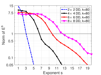
Figure 1: Norm of the power of the error propagation matrix (left: $k=40$, right: $k=80$)

Acknowledgement SG thanks the Section de Mathématiques, University of Geneva for their hospitality during his visit in early 2020. We gratefully acknowledge support from the UK Engineering and Physical Sciences Research Council Grants EP/R005591/1 (EAS) and EP/S003975/1 (SG, IGG, and EAS).

References

(1)
J-D. Benamou and B. Després.
A domain decomposition method for the Helmholtz equation and related
optimal control problems.
J. Comp. Phys., 136(1):68–82, 1997.
(2)
V. Dolean, P. Jolivet, and F. Nataf.
An introduction to domain decomposition methods: algorithms,
theory, and parallel implementation.
SIAM, 2015.
(3)
E. Efstathiou and M. J. Gander.
Why restricted additive Schwarz converges faster than additive
Schwarz.
BIT Numerical Mathematics, 43:945–959, 2003.
(4)
M. J. Gander.
Optimized Schwarz methods.
SIAM J. Numer. Anal., 44(2):699–731, 2006.
(5)
S. Gong, I. G. Graham, and E. A Spence.
Domain decomposition preconditioners for high-order discretisations
of the heterogeneous Helmholtz equation.
IMA J. Numer. Anal., https://doi.org/10.1093/imanum/draa080,
2020.
(6)
S. Gong, M.J. Gander, I. G. Graham, D. Lafontaine, and E. A Spence.
Convergence of overlapping domain decomposition methods for the
Helmholtz equation.
arXiv:2106.05218, 2021.
(7)
I. G. Graham, E. A. Spence, and E. Vainikko.
Recent results on domain decomposition preconditioning for the
high-frequency Helmholtz equation using absorption.
In Domenico Lahaye, Jok Tang, and Kees Vuik, editors, Modern
solvers for Helmholtz problems. Birkhauser 2017.
(8)
F. Hecht.
Freefem++ manual (version 3.58-1), 2019.
(9)
J-H. Kimn and M. Sarkis.
Restricted overlapping balancing domain decomposition methods and
restricted coarse problems for the Helmholtz problem.
Comput. Method Appl. Mech. Engrg., 196(8):1507–1514, 2007.
(10)
A. St-Cyr, M. J. Gander, and S. J. Thomas.
Optimized multiplicative, additive, and restricted additive Schwarz
preconditioning.
SIAM J. Sci. Comput., 29(6):2402–2425, 2007.