Functional-renormalization-group approach to classical liquids with short-range repulsion: a scheme without repulsive reference system

Abstract

The renormalization-group approaches for classical liquids in previous works require a repulsive reference such as a hard-core one when applied to systems with short-range repulsion. The need for the reference is circumvented here by using a functional renormalization group approach for integrating the hierarchical flow of correlation functions along a path of variable interatomic coupling. We introduce the cavity distribution functions to avoid the appearance of divergent terms and choose a path to reduce the error caused by the decomposition of higher order correlation functions. We demonstrate using an exactly solvable one-dimensional models that the resulting scheme yields accurate thermodynamic properties and interatomic distribution at various densities when compared to integral-equation methods such as the hypernetted chain and the Percus-Yevick equation, even in the case where our hierarchical equations are truncated with the Kirkwood superposition approximation, which is valid for low-density cases.

I Introduction

In the context of the statistical-mechanical theory for classical liquids, there is a long history for the studies of integral equations governing density correlation functions, or distribution functions Hansen and McDonald (2013). A famous and successful one is that relying on the Ornstein–Zernike (OZ) equation with approximated closures, such as the hypernetted chain (HNC) and the Percus–Yevick (PY) equation. How to systematically improve the accuracy in this framework is, however, still an open problem. The Bogoliubov–Born–Green–Kirkwood–Yvon (BBGKY) hierarchy of equations is another well-known and rigorous framework. It is, however, still a challenging problem to describe dense systems accurately with this hierarchy. For instance, precise knowledge about the lower- and higher-order distribution functions beyond the Kirkwood superposition approximation (KSA) is required to describe dense systems with the BBGKY hierarchy of equations as, truncated with KSA, it might magnify the error induced by KSA Barker and Henderson (1976) and actually shows poor results at high densities Kirkwood et al. (1950); Levesque (1966) in comparison with HNC and PY.

The renormalization group (RG) is another fundamental notion to capture properties of many-body systems, where differential equations associated with the scale transformation play the central role. The concept of RG has also been applied to the analysis of classical liquids, see, e.g., Refs. Parola and Reatto (1985); Parola et al. (1993); Parola and Reatto (1995); Parola et al. (2008, 2009); Parola and Reatto (2012); Salvino and White (1992); White and Zhang (1993, 1995); Iso and Kawana (2019); Caillol (2006, 2011); Lue and the references therein, which include the hierarchical reference theory (HRT) Parola and Reatto (1985); Parola et al. (1993); Parola and Reatto (1995); Parola et al. (2008, 2009); Parola and Reatto (2012) known as a combination of RG and thermodynamic perturbation theory, the application of Wilson’s phase-space cell method Salvino and White (1992); White and Zhang (1993, 1995), and RG with respect to the scale transformation of density Iso and Kawana (2019).

An established framework for RG is the functional renormalization group (FRG) Wegner and Houghton (1973); Wilson and Kogut (1974); Polchinski (1984); Wetterich (1993) (for reviews, see, e.g., Refs. Berges et al. (2002); Pawlowski (2007); Metzner et al. (2012); Dupuis et al. (2021)), in which the one-parameter evolution of the system is described by an exact differential equation, which is called a flow equation, for some functional. The formalism based on the effective action Wetterich (1993) being the counterpart of the bare action incorporating the thermal and quantum fluctuations is a sophisticated framework as the flow equation is described by a closed functional differential equation for the effective action, which provides systematic ways to analyze many-body systems incorporating non-perturbative effects. There are several works for the application to classical liquids Caillol (2006, 2011); Lue , where FRG becomes a framework to treat the free-energy density functional $F[\rho]$ of the particle-number density $\rho({\bf r})$, which corresponds to the effective action multiplied by the temperature. In Refs. Caillol (2006, 2011), formal aspects of FRG for classical liquids and some analytic results are presented. Some numerical demonstration in the case of the gradient expansion employed as the approximation are shown in Ref. Lue .

FRG for the calculation of density functionals, i.e., FRG formulated for density functional theory (DFT), has also been developed in the case of quantum many-body systems, as initiated in Refs. Polonyi and Sailer (2002); Schwenk and Polonyi (2004). In this direction, some numerical applications and formal extensions, which include numerical analyses of low-dimensional toy models Kemler and Braun (2013); Rentrop et al. (2015); Kemler et al. (2017); Liang et al. (2018); Yokota et al. (2019a, b) and two- and three-dimensional electron systems Yokota and Naito (2019, 2021) and extension to the case of superfluid systems Yokota et al. (2020), have been recently achieved. The approximations employed in these works are on the basis of the vertex expansion, where the functional Taylor expansion is employed and the functional flow equation is converted to a hierarchy of flow equations for density correlation functions. These studies suggest the possibility of FRG to actually contribute the improvement of accuracy of DFT.

RG approaches for classical liquids developed until now including FRG provides various ways to incorporate the effect of long-range weak force. The contribution from short-range repulsive force is, however, usually treated in an empirical and less systematic manner: Most of the works rely on the approach in which a reference system is employed to incorporate the contribution of the short-range repulsion. This approach requires the knowledge of the reference system and causes dependence of the results on the empirical choice of the reference system, albeit being successful when choosing a well-studied and well-behaved reference as suggested in the study of HNC Sumi et al. (2016).

In this paper, we develop an FRG formulation for classical liquids, where the free energy density functional is evolved along a path of variable interatomic coupling. Herein the hierarchical flow of correlation functions obtained from the vertex expansion is stabilized for a system having short-range repulsive forces by introducing cavity distribution functions instead of reference system representing the contribution of short-range repulsion. After discussing appropriate choice for the path of variable coupling, we demonstrate the performance of our approach using one-dimensional exactly solvable models. In terms of the thermodynamic properties and interatomic distribution at high densities as well as low densities, our scheme formulated at the level of KSA for the higher order correlation functions is already superior to integral-equation methods such as HNC and PY.

This paper is organized as follows: In Sec. II, we derive the flow equation for the free-energy density functional and the hierarchy of equations for the cavity distribution functions. The discussion about a suitable choice of evolution for short-range repulsion is also in there. Section III shows the numerical demonstration of our method in one-dimensional models. Section IV is devoted to the conclusion. In Appendix A, the details of the derivation of our hierarchy of equations for distribution functions are described.

II FRG and hierarchy of equations

We first summarize the formalism of the FRG for classical many-body systems. In this paper, we restrict our discussion to the case of two-body interaction and consider its evolution. The evolving two-body interaction is denoted by $v_{\lambda}({\bf r}-{\bf r}^{\prime})$, where $\lambda$ is the evolution parameter running from $0$ to $1$ and $v_{\lambda}({\bf r}-{\bf r}^{\prime})$ continuously changes with respect to $\lambda$ satisfying the boundary condition $v_{\lambda}({\bf r}-{\bf r}^{\prime})$ as $v_{\lambda=1}({\bf r}-{\bf r}^{\prime})=v({\bf r}-{\bf r}^{\prime})$ being the two-body interaction of interest. As a way to treat strong repulsive part it is possible to set the repulsive part as the initial condition $v_{\lambda=0}({\bf r}-{\bf r}^{\prime})$, but we do not introduce a reference for the repulsive part and set $v_{\lambda=0}({\bf r}-{\bf r}^{\prime})=0$. There is a freedom for the choice of the evolution toward $v_{\lambda=1}({\bf r}-{\bf r}^{\prime})$. The appropriate choice may depend on the model for $v({\bf r}-{\bf r}^{\prime})$ and approximation scheme. Let us leave the discussion about it until Sec. II.6 and focus on the derivation of the flow equation.

Let $\mu$ and $U({\bf r})$ be the chemical potential and external field, respectively. Since these quantities always appear in the form of $\beta(\mu-U({\bf r}))$ with the inverse temperature $\beta$, we introduce the notation $\overline{\psi}({\bf r})\coloneqq\beta(\mu-U({\bf r}))$. As a functional of $\overline{\psi}({\bf r})$, the grand partition functional is given by

$$\Xi_{\lambda}[\overline{\psi}]\coloneqq \sum_{N=0}^{\infty}\frac{1}{\Lambda^{3N}N!}\int_{{\bf r}_{1},\ldots,{\bf r}_{N}}e^{-\sum_{i<j}^{N}\beta v_{\lambda}({\bf r}_{i}-{\bf r}_{j})+\sum_{i=1}^{N}\overline{\psi}({\bf r}_{i})},$$ (1)

where we have introduced the short-hand notation $\int_{{\bf r}_{1},\ldots,{\bf r}_{N}}=\int d{\bf r}_{1}\cdots\int d{\bf r}_{N}$ and the de Broglie thermal wavelength $\Lambda$. From this grand partition functional, the thermodynamic potential is given by

$$\Omega_{\lambda}[\overline{\psi}]\coloneqq-\frac{1}{\beta}\ln\Xi_{\lambda}[\overline{\psi}],$$ (2)

which plays the role of the generating functional for the density correlation functions. The Helmholtz free energy is defined by the Legendre transformation of $\Omega_{\lambda}[\overline{\psi}]$:

$$F_{\lambda}[\rho_{\rm v}] \coloneqq\max_{\overline{\psi}}\left[\Omega_{\lambda}[\overline{\psi}]+\frac{1}{\beta}\int_{{\bf r}}\rho_{\rm v}({\bf r})\overline{\psi}({\bf r})\right]$$

$$=\Omega_{\lambda}[\overline{\psi}_{\max,\lambda}[\rho_{\rm v}]]+\frac{1}{\beta}\int_{{\bf r}}\rho_{\rm v}({\bf r})\overline{\psi}_{\max,\lambda}[\rho_{\rm v}]({\bf r}),$$ (3)

where the variable $\rho_{\rm v}({\bf r})$ stands for the particle-number density and $\overline{\psi}_{\max,\lambda}[\rho_{\rm v}]$ is given through

$$-\left.\frac{\delta\beta\Omega_{\lambda}[\overline{\psi}]}{\delta\overline{\psi}({\bf r})}\right|_{\overline{\psi}=\overline{\psi}_{\max,\lambda}[\rho_{\rm v}]}=\rho_{\rm v}({\bf r}),$$ (4)

and satisfies

$$\frac{\delta\beta F_{\lambda}[\rho_{\rm v}]}{\delta\rho_{\rm v}({\bf r})}=\overline{\psi}_{\max,\lambda}[\rho_{\rm v}]({\bf r}).$$ (5)

These relations suggest that $\overline{\psi}_{\max,\lambda}[\rho_{\rm v}]({\bf r})$ is the external field giving the density $\rho_{\rm v}({\bf r})$. Conversely speaking, for a given external field $\overline{\psi}_{\rm given}({\bf r})$, $\rho_{\rm v}({\bf r})$ is determined from $\overline{\psi}_{\max,\lambda}[\rho_{\rm v}]({\bf r})=\overline{\psi}_{\rm given}({\bf r})$.

II.1 Flow equation

The evolution of $F_{\lambda}[\rho_{\rm v}]$ with respect to $\lambda$ can be described by a flow equation in a closed form for $\beta F_{\lambda}[\rho_{\rm v}]$ as follows:

$$\partial_{\lambda}\beta F_{\lambda}[\rho_{\rm v}]= \frac{1}{2}\int_{{\bf r},{\bf r}^{\prime}}\partial_{\lambda}\beta v_{\lambda}({\bf r}-{\bf r}^{\prime})\left(\rho_{\rm v}({\bf r})\rho_{\rm v}({\bf r}^{\prime})+\left(\frac{\delta^{2}\beta F_{\lambda}}{\delta\rho_{\rm v}\delta\rho_{\rm v}}\right)^{-1}[\rho_{\rm v}]({\bf r},{\bf r}^{\prime})-\rho_{\rm v}({\bf r})\delta({\bf r}-{\bf r}^{\prime})\right),$$ (6)

which we will derive shortly. Following this flow equation, $\beta F_{\lambda}[\rho_{\rm v}]$ evolves in the functional space as illustrated in Fig. 1, where the path of the evolution depends on the choice of $\beta v_{\lambda}({\bf r}-{\bf r}^{\prime})$. A similar form of the flow equation is known for quantum cases Schwenk and Polonyi (2004); Kemler and Braun (2013); Kemler et al. (2017); Yokota et al. (2019a); Yokota and Naito (2019).

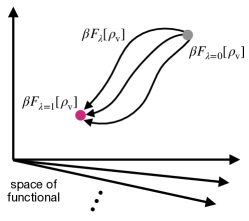
Figure 1: Schematic picture of the evolution of $\beta F_{\lambda}[\rho_{\rm v}]$. The different paths correspond to different choices of $\beta v_{\lambda}({\bf r}-{\bf r}^{\prime})$.

The derivation of Eq. (6) is as follows: The derivative of Eq. (II) with respect to $\lambda$ together with Eq. (4) leads to

$$\partial_{\lambda}\beta F_{\lambda}[\rho_{\rm v}]=(\partial_{\lambda}\beta\Omega_{\lambda})[\overline{\psi}_{\max,\lambda}[\rho_{\rm v}]].$$ (7)

Note that the partial derivative on the right-hand side does not act on the argument of $\Omega_{\lambda}$, i.e., $\overline{\psi}_{\max,\lambda}[\rho_{\rm v}]$. By use of the definitions Eqs. (1) and (2), Eq. (7) is rewritten as

$$\partial_{\lambda}\beta\Omega_{\lambda}[\overline{\psi}_{\max,\lambda}[\rho_{\rm v}]]= \frac{1}{\Xi_{\lambda}[\overline{\psi}_{\max,\lambda}[\rho_{\rm v}]]}\sum_{N=0}^{\infty}\frac{1}{\Lambda^{3N}N!}\int_{{\bf r}_{1},\cdots,{\bf r}_{N}}\sum_{i<j}^{N}\partial_{\lambda}\beta v_{\lambda}({\bf r}_{i}-{\bf r}_{j})e^{-\sum_{i^{\prime}<j^{\prime}}^{N}\beta v_{\lambda}({\bf r}_{i^{\prime}}-{\bf r}_{j^{\prime}})+\sum_{i^{\prime}=1}^{N}\overline{\psi}_{\max,\lambda}[\rho_{\rm v}]({\bf r}_{i^{\prime}})}$$

$$= \int_{{\bf r},{\bf r}^{\prime}}\partial_{\lambda}\beta v_{\lambda}({\bf r}-{\bf r}^{\prime})\left\langle\sum_{i<j}^{\hat{N}}\delta({\bf r}-\hat{\bf r}_{i})\delta({\bf r}^{\prime}-\hat{\bf r}_{j})\right\rangle_{\lambda,\overline{\psi}_{\max,\lambda}[\rho_{\rm v}]}$$

$$= \frac{1}{2}\int_{{\bf r},{\bf r}^{\prime}}\partial_{\lambda}\beta v_{\lambda}({\bf r}-{\bf r}^{\prime})\left\langle\hat{\rho}({\bf r})\hat{\rho}({\bf r}^{\prime})-\hat{\rho}({\bf r})\delta({\bf r}-\hat{\bf r}^{\prime})\right\rangle_{\lambda,\overline{\psi}_{\max,\lambda}[\rho_{\rm v}]},$$ (8)

where

$$\left\langle\cdots\right\rangle_{\lambda,\overline{\psi}}= \frac{1}{\Xi_{\lambda}[\overline{\psi}]}\sum_{N=0}^{\infty}\frac{1}{\Lambda^{3N}N!}\int_{{\bf r}_{1},\cdots,{\bf r}_{N}}\cdots e^{-\sum_{k<l}^{N}\beta v_{\lambda}({\bf r}_{k}-{\bf r}_{l})+\sum_{k=1}^{N}\overline{\psi}({\bf r}_{k})},$$ (9)

and $\hat{\rho}({\bf r})=\sum_{i=1}^{\hat{N}}\delta(\hat{\bf r}_{i}-{\bf r})$ with $\hat{N}$ and $\hat{\bf r}$ being variables to be averaged. From Eqs. (1), (2), and (4), one finds

$$\left\langle\hat{\rho}({\bf r})\right\rangle_{\lambda,\overline{\psi}_{\max,\lambda}[\rho_{\rm v}]}= \rho_{\rm v}({\bf r}),$$ (10)

$$\left\langle\hat{\rho}({\bf r})\hat{\rho}({\bf r}^{\prime})\right\rangle_{\lambda,\overline{\psi}_{\max,\lambda}[\rho_{\rm v}]}= \rho_{\rm v}({\bf r})\rho_{\rm v}({\bf r}^{\prime})-\left.\frac{\delta^{2}\beta\Omega_{\lambda}[\overline{\psi}]}{\delta\overline{\psi}({\bf r})\delta\overline{\psi}({\bf r}^{\prime})}\right|_{\overline{\psi}=\overline{\psi}_{\max,\lambda}[\rho_{\rm v}]}.$$ (11)

As shown from the derivative of Eq. (4) with respect to $\overline{\psi}_{\max,\lambda}(\bf r)$ and the derivative of Eq. (5) with respect to $\rho_{\rm v}({\bf r})$, the following inverse relation holds:

$$\left(\frac{\delta^{2}\beta F_{\lambda}}{\delta\rho_{\rm v}\delta\rho_{\rm v}}\right)^{-1}[\rho_{\rm v}]({\bf r},{\bf r}^{\prime})=-\left.\frac{\delta^{2}\beta\Omega_{\lambda}[\overline{\psi}]}{\delta\overline{\psi}({\bf r})\delta\overline{\psi}({\bf r}^{\prime})}\right|_{\overline{\psi}=\overline{\psi}_{\max,\lambda}[\rho_{\rm v}]},$$ (12)

where the left-hand side is defined through

$$\int_{{\bf r}^{\prime\prime}}\left(\frac{\delta^{2}\beta F_{\lambda}}{\delta\rho_{\rm v}\delta\rho_{\rm v}}\right)^{-1}[\rho_{\rm v}]({\bf r},{\bf r}^{\prime\prime})\frac{\delta^{2}\beta F_{\lambda}[\rho_{\rm v}]}{\delta\rho_{\rm v}({\bf r}^{\prime\prime})\delta\rho_{\rm v}({\bf r}^{\prime})}=\delta({\bf r}-{\bf r}^{\prime}).$$ (13)

From Eq. (7) together with Eqs. (II.1) and (10)-(12), we finally obtain Eq. (6).

II.2 Vertex expansion

In principle, $\beta F_{\lambda}[\rho_{\rm v}]$, and thus all the thermodynamic quantities and correlation functions, are obtained by solving Eq. (6) only. It is, however, nontrivial whether Eq. (6) can be used practically. In particular, the functional equation is hard to treat numerically in a direct manner as the space of the argument $\rho_{\rm v}({\bf r})$ is computationally huge, and introduction of some approximation is practically needed. Here, we employ the vertex expansion, in which the functional Taylor expansion around

$$\rho_{\rm v}({\bf r})=\rho({\bf r})$$ (14)

with $\rho({\bf r})$ being some density of interest, and truncate the expansion at some order to realize numerical calculation. Since the derivative coefficients of $\beta F_{\lambda}[\rho_{\rm v}]$ are related to correlation functions, the hierarchy of flow equations can be written in terms of the correlation functions. Let us introduce the $m$-particle density:

$$\rho^{(m)}_{\lambda}({\bf r}_{1},\ldots,{\bf r}_{m})=\left\langle\prod_{i=1}^{m}\left(\hat{\rho}({\bf r}_{i})-\sum_{j=1}^{i-1}\delta({\bf r}_{j}-{\bf r}_{i})\right)\right\rangle_{\lambda,\overline{\psi}_{\max,\lambda}[\rho]}.$$ (15)

Through the derivations as summarized in Appendix A, the following hierarchy of the flow equations are obtained:

$$\partial_{\lambda}\beta F_{\lambda}=\frac{1}{2}\int_{{\bf r},{\bf r}^{\prime}}\partial_{\lambda}\beta v_{\lambda}({\bf r}-{\bf r}^{\prime})\rho^{(2)}_{\lambda}({\bf r},{\bf r}^{\prime}),$$ (16)

$$\partial_{\lambda}\rho_{\lambda}^{(m)}({\bf r}_{1},\ldots,{\bf r}_{m})+\sum_{i<j}^{m}\partial_{\lambda}\left[\beta v_{\lambda}({\bf r}_{i}-{\bf r}_{j})\right]\rho_{\lambda}^{(m)}({\bf r}_{1},\ldots,{\bf r}_{m})$$

$$\quad=\int_{{\bf r}}\left[\rho^{(m+1)}_{\lambda}({\bf r}_{1},\ldots,{\bf r}_{m},{\bf r})-\rho({\bf r})\rho^{(m)}_{\lambda}({\bf r}_{1},\ldots,{\bf r}_{m})\right]\partial_{\lambda}\overline{\psi}_{\max,\lambda}({\bf r})$$

$$\qquad+\rho^{(m)}_{\lambda}({\bf r}_{1},\ldots,{\bf r}_{m})\sum_{i=1}^{m}\partial_{\lambda}\overline{\psi}_{\max,\lambda}({\bf r}_{i})-\int_{{\bf r}}\sum_{i=1}^{m}\partial_{\lambda}\left[\beta v_{\lambda}({\bf r}-{\bf r}_{i})\right]\rho^{(m+1)}_{\lambda}({\bf r},{\bf r}_{1},\ldots,{\bf r}_{m})$$

$$\qquad-\frac{1}{2}\int_{{\bf r},{\bf r}^{\prime}}\partial_{\lambda}\left[\beta v_{\lambda}({\bf r}-{\bf r}^{\prime})\right]\left[\rho^{(m+2)}_{\lambda}({\bf r},{\bf r}^{\prime},{\bf r}_{1},\ldots,{\bf r}_{m})-\rho^{(2)}_{\lambda}({\bf r},{\bf r}^{\prime})\rho^{(m)}_{\lambda}({\bf r}_{1},\ldots,{\bf r}_{m})\right],$$ (17)

with $m\geq 1$, $\beta F_{\lambda}\coloneqq\beta F_{\lambda}[\rho]$, and $\overline{\psi}_{\max,\lambda}({\bf r})\coloneqq\overline{\psi}_{\max,\lambda}[\rho]({\bf r})$. Note that in the case of $m=1$, Eq. (II.2) is regarded as the flow equation for $\overline{\psi}_{\max,\lambda}({\bf r})$ rather than that for $\rho^{(1)}_{\lambda}({\bf r})$ since we fix $\rho({{\bf r}})$ during the flow and $\rho^{(1)}_{\lambda}({\bf r})$ always satisfies $\partial_{\lambda}\rho^{(1)}_{\lambda}({\bf r})=\partial_{\lambda}\rho({\bf r})=0$.

II.3 Cavity distribution function

There still remains an obstacle for numerical calculation. If $v_{\lambda}({\bf r}-{\bf r}^{\prime})$ has infinitely strong repulsion, Eqs. (16) and (II.2) seem to have divergent parts. However, this seeming divergence can be eliminated by introducing the cavity distribution function Hansen and McDonald (2013). The $m$-particle cavity distribution function Meeron and Siegert (1968) is defined by

$$y^{(m)}_{\lambda}({\bf r}_{1},\ldots,{\bf r}_{m})=e^{\beta\sum_{i<j}^{m}v_{\lambda}({\bf r}_{i}-{\bf r}_{j})}g^{(m)}_{\lambda}({\bf r}_{1},\ldots,{\bf r}_{m}),$$ (18)

where $g^{(m)}_{\lambda}({\bf r}_{1},\cdots,{\bf r}_{m})$ is the $m$-particle distribution functions, which are defined by the normalization of $\rho^{(m)}_{\lambda}({\bf r}_{1},\ldots,{\bf r}_{m})$ with densities:

$$g^{(m)}_{\lambda}({\bf r}_{1},\ldots,{\bf r}_{m})=\frac{\rho^{(m)}_{\lambda}({\bf r}_{1},\ldots,{\bf r}_{m})}{\Pi_{i=1}^{m}\rho({\bf r}_{i})}.$$ (19)

The physical meaning of the cavity distribution function is revealed by remembering Eqs. (9) and (15), which give

$$\rho^{(m)}_{\lambda}({\bf r}_{1},\ldots,{\bf r}_{m})= \frac{1}{\Xi_{\lambda}[\overline{\psi}]}\sum_{N=m}^{\infty}\frac{1}{\Lambda^{3N}(N-m)!}\int_{{\bf r}_{m+1},\cdots,{\bf r}_{N}}$$

$$\times e^{-\sum_{k<l}^{N}\beta v_{\lambda}({\bf r}_{k}-{\bf r}_{l})+\sum_{k=1}^{N}\overline{\psi}({\bf r}_{k})}.$$ (20)

Rewriting Eq. (18) using Eqs. (19) and (II.3), one finds that the factor $\exp(-\sum_{k<l}^{m}\beta v_{\lambda}({\bf r}_{k}-{\bf r}_{l}))$ coming from the interaction among the $m$ particles is canceled by the exponential factor in Eq. (18). Therefore, $y^{(m)}_{\lambda}({\bf r}_{1},\ldots,{\bf r}_{m})$ is proportional to the probability that the $m$ particles which do not interact with each other but interact with other particles are at ${\bf r}_{1},\ldots,{\bf r}_{m}$. Particularly in the case of hard spheres with a diameter $d$, the $m$ particles play an equivalent role to that of cavities with radius at least $d$ Meeron and Siegert (1968). Since the $m$ particles can overlap with each other, $y^{(m)}_{\lambda}({\bf r}_{1},\ldots,{\bf r}_{m})$ can take a finite value for $|{\bf r}_{i}-{\bf r}_{j}|<d$ with $i\neq j$ even in the hard-sphere case in contrast to $g^{(m)}_{\lambda}({\bf r}_{1},\ldots,{\bf r}_{m})$.

Actually, the flow equations are rewritten as follows:

$$\partial_{\lambda}\beta F_{\lambda}=-\frac{1}{2}\int_{{\bf r},{\bf r^{\prime}}}\rho({\bf r})\rho({\bf r}^{\prime})\left[\partial_{\lambda}e^{-\beta v_{\lambda}({\bf r}-{\bf r}^{\prime})}\right]y^{(2)}_{\lambda}({\bf r},{\bf r}^{\prime}),$$ (21)

$$\partial_{\lambda}y_{\lambda}^{(m)}({\bf r}_{1},\ldots,{\bf r}_{m})$$

$$\qquad=\int_{{\bf r}}\rho({\bf r})\left[e^{-\beta\sum_{i}^{m}v_{\lambda}({\bf r}_{i}-{\bf r})}y^{(m+1)}_{\lambda}({\bf r}_{1},\ldots,{\bf r}_{m},{\bf r})-y^{(m)}_{\lambda}({\bf r}_{1},\ldots,{\bf r}_{m})\right]\partial_{\lambda}\overline{\psi}_{\max,\lambda}({\bf r})$$

$$\qquad+y^{(m)}_{\lambda}({\bf r}_{1},\ldots,{\bf r}_{m})\sum_{i=1}^{m}\partial_{\lambda}\overline{\psi}_{\max,\lambda}({\bf r}_{i})+\int_{{\bf r}}\rho({\bf r})\left[\partial_{\lambda}e^{-\sum_{i}^{m}\beta v_{\lambda}({\bf r}_{i}-{\bf r})}\right]y^{(m+1)}_{\lambda}({\bf r},{\bf r}_{1},\ldots,{\bf r}_{m})$$

$$\qquad+\frac{1}{2}\int_{{\bf r},{\bf r}^{\prime}}\rho({\bf r})\rho({\bf r}^{\prime})\left[\partial_{\lambda}e^{-\beta v_{\lambda}({\bf r}-{\bf r}^{\prime})}\right]$$

$$\qquad\times\left[e^{-\sum_{i}^{m}\beta v_{\lambda}({\bf r}_{i}-{\bf r})-\sum_{i}^{m}\beta v_{\lambda}({\bf r}_{i}-{\bf r}^{\prime})}y^{(m+2)}_{\lambda}({\bf r},{\bf r}^{\prime},{\bf r}_{1},\ldots,{\bf r}_{m})-y^{(2)}_{\lambda}({\bf r},{\bf r}^{\prime})y^{(m)}_{\lambda}({\bf r}_{1},\ldots,{\bf r}_{m})\right],$$ (22)

in which $v_{\lambda}({\bf r}-{\bf r}^{\prime})$ always appears in the form of $e^{-\beta v_{\lambda}({\bf r}-{\bf r}^{\prime})}$ and there is no divergence due to the strong repulsion. Therefore, these equations enable one to treat the short-range strong repulsion as well as the long-range attraction on the same footing. In passing, each term in the right-hand side of Eq. (II.3) is interpreted as follows: The first and second terms are derived from the change of $\overline{\psi}_{\max,\lambda}({\bf r})$, i.e., the change of the chemical potential to fix the density. The third and fourth terms reflect the changes of the interactions between any one of particles on ${\bf r}_{1},\ldots,{\bf r}_{m}$ and another one and between two particles other than particles on ${\bf r}_{1},\ldots,{\bf r}_{m}$, respectively. Since the cavity distribution function $y_{\lambda}^{(m)}({\bf r}_{1},\ldots,{\bf r}_{m})$ is interpreted as the distribution when the interactions among particles on ${\bf r}_{1},\ldots,{\bf r}_{m}$ are switched off Hansen and McDonald (2013), there is no term reflecting the changes of interactions among them, such as the second term in the left-hand side of Eq. (II.2).

II.4 Truncation

Although Eqs. (21) and (II.3) are exact, they depend on higher-order distribution functions to form infinite hierarchy of coupled equations and truncation at some order is needed for practical use. Some approximate relation connecting distribution functions of different order is required to close the hierarchy of equations. Among many approximations proposed for $g^{(m)}_{\lambda}({\bf r}_{1},\ldots,{\bf r}_{m})$, preferable ones for our formulation are those guaranteeing the finiteness of $y^{(m)}_{\lambda}({\bf r}_{1},\ldots,{\bf r}_{m})$ in the case of strong repulsion. A naive and suitable one is KSA, which exactly holds at low-density limit. For simplicity, we consider KSA for $y^{(3)}_{\lambda}({\bf r}_{1},{\bf r}_{2},{\bf r}_{3})$ and $y^{(4)}_{\lambda}({\bf r}_{1},{\bf r}_{2},{\bf r}_{3},{\bf r}_{4})$, on which the second order flow equation depends:

$$y^{(3)}_{\lambda}({\bf r}_{1},{\bf r}_{2},{\bf r}_{3}) \approx y^{(2)}_{\lambda}({\bf r}_{1},{\bf r}_{2})y^{(2)}_{\lambda}({\bf r}_{2},{\bf r}_{3})y^{(2)}_{\lambda}({\bf r}_{3},{\bf r}_{1})+\mathcal{O}(\rho),$$ (23)

$$y^{(4)}_{\lambda}({\bf r}_{1},{\bf r}_{2},{\bf r}_{3},{\bf r}_{4}) \approx\frac{y^{(3)}_{\lambda}({\bf r}_{1},{\bf r}_{2},{\bf r}_{3})y^{(3)}_{\lambda}({\bf r}_{2},{\bf r}_{3},{\bf r}_{4})y^{(3)}_{\lambda}({\bf r}_{3},{\bf r}_{4},{\bf r}_{1})y^{(3)}_{\lambda}({\bf r}_{4},{\bf r}_{1},{\bf r}_{2})}{y^{(2)}_{\lambda}({\bf r}_{1},{\bf r}_{2})y^{(2)}_{\lambda}({\bf r}_{1},{\bf r}_{3})y^{(2)}_{\lambda}({\bf r}_{1},{\bf r}_{4})y^{(2)}_{\lambda}({\bf r}_{2},{\bf r}_{3})y^{(2)}_{\lambda}({\bf r}_{2},{\bf r}_{4})y^{(2)}_{\lambda}({\bf r}_{3},{\bf r}_{4})}+\mathcal{O}(\rho)$$

$$\approx y^{(2)}_{\lambda}({\bf r}_{1},{\bf r}_{2})y^{(2)}_{\lambda}({\bf r}_{1},{\bf r}_{3})y^{(2)}_{\lambda}({\bf r}_{1},{\bf r}_{4})y^{(2)}_{\lambda}({\bf r}_{2},{\bf r}_{3})y^{(2)}_{\lambda}({\bf r}_{2},{\bf r}_{4})y^{(2)}_{\lambda}({\bf r}_{3},{\bf r}_{4})+\mathcal{O}(\rho).$$ (24)

A naive way to improve the accuracy of the calculation is taking higher-order flow equations into account. However, it may be time consuming to solve higher-order flow equations since the number of arguments for the distribution functions increases. Another approach for the improvement of the accuracy is to find more accurate approximation beyond KSA. There are many studies for the correction to KSA GROUBA et al. (2004). For example, according to Ref. Abe (1959), the correction term to $y^{(3)}_{\lambda}({\bf r}_{1},{\bf r}_{2},{\bf r}_{3})$ up to $\mathcal{O}(\rho)$ is given by

$$y^{(3)}_{\lambda}({\bf r}_{1},{\bf r}_{2},{\bf r}_{3})\approx y^{(2)}_{\lambda}({\bf r}_{1},{\bf r}_{2})y^{(2)}_{\lambda}({\bf r}_{2},{\bf r}_{3})y^{(2)}_{\lambda}({\bf r}_{3},{\bf r}_{1})e^{\rho\int_{{\bf r}}h_{\lambda}^{(2)}({\bf r}_{1},{\bf r})h_{\lambda}^{(2)}({\bf r}_{2},{\bf r})h_{\lambda}^{(2)}({\bf r}_{3},{\bf r})}+\mathcal{O}(\rho^{2}),$$ (25)

where $h_{\lambda}^{(2)}({\bf r},{\bf r}^{\prime})=g_{\lambda}^{(2)}({\bf r},{\bf r}^{\prime})-1$ is the total correlation function, in which $g_{\lambda}^{(2)}({\bf r},{\bf r}^{\prime})$ is related to $y_{\lambda}^{(2)}({\bf r},{\bf r}^{\prime})$ through Eq. (18). The convolution approximation Ichimaru (1970) is another approximation for $g^{(3)}_{\lambda}({\bf r}_{1},{\bf r}_{2},{\bf r}_{3})$. Unfortunately, this approximation does not guarantee the finiteness of $y^{(3)}_{\lambda}({\bf r}_{1},{\bf r}_{2},{\bf r}_{3})$ since the core condition, which means that $g^{(3)}_{\lambda}({\bf r}_{1},{\bf r}_{2},{\bf r}_{3})$ vanishes if any of $|{\bf r}_{i}-{\bf r}_{j}|$ ($1\leq i<j\leq 3$) is lesser than the hard-core diameter for hard-core systems, is not satisfied.

II.5 Homogeneous cases

In Sec. III, we will apply the formalism to homogeneous liquids. For this purpose, we rewrite the flow equations for the homogeneous case. In this case, $\rho({\bf r})$ and $\overline{\psi}_{\max,\lambda}({\bf r})$ do not depend on ${\bf r}$ and $y^{(m)}_{\lambda}({\bf r}_{1},\ldots,{\bf r}_{m})$ only depends on ${\bf r}_{1}-{\bf r}_{m},\ldots,{\bf r}_{m-1}-{\bf r}_{m}$; we denote $\rho({\bf r})$ and $\overline{\psi}_{\max,\lambda}({\bf r})$ as $\rho$ and $\overline{\psi}_{\max,\lambda}$, respectively, and $y^{(m)}_{\lambda}({\bf r}_{1},\ldots,{\bf r}_{m})$ as $y^{(m)}_{\lambda}({\bf r}_{1},\ldots,{\bf r}_{m-1})$ regarding ${\bf r}_{m}$ as the original point. Then, Eqs. (21) and (II.3) are respectively reduced to

$$\partial_{\lambda}\frac{\beta F_{\lambda}}{N}=-\frac{\rho}{2}\int_{{\bf r}}\left[\partial_{\lambda}e^{-\beta v_{\lambda}({\bf r})}\right]y^{(2)}_{\lambda}({\bf r}),$$ (26)

$$\partial_{\lambda}\ln y_{\lambda}^{(m)}({\bf r}_{1},\ldots,{\bf r}_{m-1})$$

$$=\partial_{\lambda}\overline{\psi}_{{\max},\lambda}\left(m+\rho\int_{{\bf r}}\left[e^{-\beta\sum_{i}^{m-1}v_{\lambda}({\bf r}_{i}-{\bf r})-\beta v_{\lambda}({\bf r})}\frac{y^{(m+1)}_{\lambda}({\bf r}_{1},\ldots,{\bf r}_{m-1},{\bf r})}{y^{(m)}_{\lambda}({\bf r}_{1},\ldots,{\bf r}_{m-1})}-1\right]\right)$$

$$\quad+\rho\int_{{\bf r}}\partial_{\lambda}\left[e^{-\beta\sum_{i}^{m-1}v_{\lambda}({\bf r}_{i}-{\bf r})-\beta v_{\lambda}({\bf r})}\right]\frac{y^{(m+1)}_{\lambda}({\bf r},{\bf r}_{1},\ldots,{\bf r}_{m-1})}{y^{(m)}_{\lambda}({\bf r}_{1},\ldots,{\bf r}_{m-1})}$$

$$\quad+\frac{\rho^{2}}{2}\int_{{\bf r},{\bf r}^{\prime}}\partial_{\lambda}\left[e^{-\beta v_{\lambda}({\bf r}-{\bf r}^{\prime})}\right]y^{(2)}_{\lambda}({\bf r}-{\bf r}^{\prime})$$

$$\quad\times\left[e^{-\beta\sum_{i}^{m-1}v_{\lambda}({\bf r}_{i}-{\bf r})-\beta\sum_{i}^{m-1}v_{\lambda}({\bf r}_{i}-{\bf r}^{\prime})-\beta v_{\lambda}({\bf r})-\beta v_{\lambda}({\bf r}^{\prime})}\frac{y^{(m+2)}_{\lambda}({\bf r},{\bf r}^{\prime},{\bf r}_{1},\ldots,{\bf r}_{m-1})}{y^{(2)}_{\lambda}({\bf r}-{\bf r}^{\prime})y^{(m)}_{\lambda}({\bf r}_{1},\ldots,{\bf r}_{m-1})}-1\right],$$ (27)

where $N=\rho\int d{\bf r}$ is the total particle number. In this case, the flow equation for $\overline{\psi}_{{\max},\lambda}$ is explicitly derived from Eq. (II.5) for $m=1$ and $y^{(1)}_{\lambda}=1$:

$$\partial_{\lambda}\overline{\psi}_{{\max},\lambda}=-\frac{\rho\int_{{\bf r}}\partial_{\lambda}\left[e^{-\beta v_{\lambda}({\bf r})}\right]y^{(2)}_{\lambda}({\bf r})\left(1+\frac{\rho}{2}\int_{{\bf r}^{\prime}}\left[e^{-\beta v_{\lambda}({\bf r}+{\bf r}^{\prime})-\beta v_{\lambda}({\bf r}^{\prime})}\frac{y^{(3)}_{\lambda}({\bf r}+{\bf r}^{\prime},{\bf r}^{\prime})}{y^{(2)}_{\lambda}({\bf r})}-1\right]\right)}{1+\rho\int_{{\bf r}}\left[e^{-\beta v_{\lambda}({\bf r})}y^{(2)}_{\lambda}({\bf r})-1\right]}.$$ (28)

In homogeneous systems, the leading order of the density expansion for $\omega_{\lambda}({\bf r}_{1})=\ln y_{\lambda}({\bf r}_{1})$ is known as Hansen and McDonald (2013)

$$\omega_{\lambda}({\bf r}_{1})=\rho\int_{{\bf r}}f_{\lambda}({\bf r}_{1}-{\bf r})f_{\lambda}({\bf r})$$ (29)

with the Mayer function $f_{\lambda}({\bf r})=e^{-\beta v_{\lambda}({\bf r})}-1$. This can be reproduced from Eqs. (28) and (II.5) for $m=2$. If we ignore the $\lambda$ dependence in the right-hand sides of Eqs. (28) and (II.5) for $m=2$ except for $\partial_{\lambda}\left[e^{-\beta v_{\lambda}({\bf r})}\right]$ and $\partial_{\lambda}\left[e^{-\beta v_{\lambda}({\bf r}-{\bf r}^{\prime})}\right]$, Eqs. (28) and (II.5) for $m=2$ are approximated as follows:

$$\partial_{\lambda}\overline{\psi}_{{\max},\lambda} \approx-\rho\int_{{\bf r}}\partial_{\lambda}\left[e^{-\beta v_{\lambda}({\bf r})}\right],$$ (30)

$$\partial_{\lambda}\omega_{\lambda}({\bf r}_{1}) \approx 2\partial_{\lambda}\overline{\psi}_{{\max},\lambda}+\rho\int_{{\bf r}}\partial_{\lambda}\left[e^{-\beta v_{\lambda}({\bf r}_{1}-{\bf r})-\beta v_{\lambda}({\bf r})}\right].$$ (31)

Inserting Eq. (30) into Eq. (31) and integrating Eq. (31) with respect to $\lambda$, we have Eq. (29). By considering the $\lambda$ dependence of other factors in addition to $\partial_{\lambda}\left[e^{-\beta v_{\lambda}({\bf r})}\right]$ and $\partial_{\lambda}\left[e^{-\beta v_{\lambda}({\bf r}-{\bf r}^{\prime})}\right]$, the higher-order contributions in the density expansion are incorporated in our flow equations.

II.6 Setting of the evolution to treat hard core

In principle, results do not depend on the choice of $v_{\lambda}({\bf r}-{\bf r}^{\prime})$ during the flow if the flow equations are exactly treated. The introduction of truncation, however, causes the dependence and one should discuss appropriate settings for $v_{\lambda}({\bf r}-{\bf r}^{\prime})$. Moreover, some choice of $v_{\lambda}({\bf r}-{\bf r}^{\prime})$ causes breakdown of the numerical calculation. Let us give a discussion about the choice of $v_{\lambda}({\bf r}-{\bf r}^{\prime})$ for a two-body interaction having a repulsive core in the case of employing KSA.

A naive choice may be the adiabatic-connection-like form:

$$v_{\lambda}({\bf r}-{\bf r}^{\prime})=\lambda v({\bf r}-{\bf r}^{\prime}).$$ (32)

This choice is, however, problematic in the case of the presence of a repulsive core. For simplicity, let us consider the case of a hard sphere with a diameter $\sigma$. Under the choice of Eq. (32), we have

$$e^{-\beta v_{\lambda}({\bf r}-{\bf r}^{\prime})}=\begin{cases}1&\lambda=0,\\ \theta(|{\bf r}-{\bf r}^{\prime}|-\sigma)&\lambda>0,\end{cases}$$ (33)

which shows the factors such as $e^{-\beta v_{\lambda}({\bf r}-{\bf r}^{\prime})}$ appearing in the flow equations (26) and (II.5) suddenly changes as $\lambda$ departs from $0$ and particularly the divergences of the factors $\partial_{\lambda}e^{-\beta v_{\lambda}({\bf r}-{\bf r}^{\prime})}$ occur at $\lambda=0$. Such divergences are hard to treat in the numerical calculation.

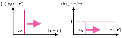
Figure 2: Visual representation of (a) $v_{\lambda}({\bf r}-{\bf r}^{\prime})$ and (b) $e^{-\beta v_{\lambda}({\bf r}-{\bf r}^{\prime})}$ under the evolution given by Eq. (34).

Our proposal for a possible choice not only circumventing this problem but also contributing to the improvement of the accuracy with KSA is the following one:

$$v_{\lambda}({\bf r}-{\bf r}^{\prime})=\begin{cases}\infty&|{\bf r}-{\bf r}^{\prime}|<\lambda\sigma,\\ 0&|{\bf r}-{\bf r}^{\prime}|\geq\lambda\sigma,\end{cases}$$ (34)

which is represented visually in Fig. 2. This evolution represents that the repulsive core is gradually taken from short-range region and, in this sense, is regarded as a choice inspired by the notion of RG. Hereafter, we call the choice the RG-inspired flow. In this case, the exponential factor and the derivative become

$$e^{-\beta v_{\lambda}({\bf r}-{\bf r}^{\prime})}= \theta(|{\bf r}-{\bf r}^{\prime}|-\lambda\sigma),$$ (35)

$$\partial_{\lambda}e^{-\beta v_{\lambda}({\bf r}-{\bf r}^{\prime})}= -\sigma\delta(|{\bf r}-{\bf r}^{\prime}|-\lambda\sigma).$$ (36)

Figure 2 also shows the evolution of $e^{-\beta v_{\lambda}({\bf r}-{\bf r}^{\prime})}$. Although a delta function appears in $\partial_{\lambda}e^{-\beta v_{\lambda}({\bf r}-{\bf r}^{\prime})}$, this factor always appears in the integrands of spatial integrals in Eqs. (26) and (II.5) and does not cause divergence in the flow equations. This choice also has an advantage for the accuracy of the calculation with KSA. Since the only dimensionless parameter of the hard-sphere fluid is the packing fraction, a system composed of hard spheres with a small diameter can be viewed as a low-density system. In addition, the RG-inspired flow is equivalent to considering an evolving packing fraction $\eta_{\lambda}=\rho V_{\rm HS}(\lambda\sigma)$ with $V_{\rm HS}(\lambda\sigma)$ being the volume of a hard sphere having a diameter $\lambda\sigma$. Therefore, it is guaranteed that the flow equations with KSA becomes accurate at least small $\lambda$ since KSA is accurate in low-density cases. Although KSA holds only for low-density cases, the property that the flow is accurate at least near the starting point $\lambda=0$ may contribute to the improvement of the accuracy of FRG in moderate and high densities.

It is conceivable to improve the accuracy by optimizing the evolution with a help of the principle of minimal sensitivity (PMS) Canet et al. (2003). In the PMS, one uses the exact condition by which the results do not depend on the choice of the evolution, which in our case, corresponds to generalizing the evolution of $\beta v_{\lambda}({\bf r}-{\bf r}^{\prime})$ for finding a stationary path.

The derivation of the flow equations for cavity distribution functions and the ideas for truncation and choice of the flow have been presented in this section. In the next section, the accuracy of our method will be assessed through applications to exactly solvable models.

III Demonstration in one-dimensional liquids

In this section, we apply the flow equations obtained in the previous section to one-dimensional exactly solvable models to investigate the accuracy. In particular, our results are compared to those obtained by HNC and PY.

III.1 Model

For the purpose of investigating the accuracy of our method, an application to a model for which exact solutions are obtained is desirable. We employ a one-dimensional fluid composed of hard rods with an attractive force Archer et al. (2017), whose interaction is described by

$$\beta v(r)=\begin{cases}\infty&|r|<\sigma\\ -z_{\rm p}(\sigma+\sigma_{\rm p}-|r|)&\sigma\leq|r|<\sigma+\sigma_{\rm p}\\ 0&\sigma+\sigma_{\rm p}\leq|r|\end{cases},$$ (37)

where $\sigma\geq 0$ is the diameter of a hard rod and the parameters for the attractive force satisfies $z_{\rm p}\geq 0$ and $\sigma_{\rm p}\geq 0$.

It is known that exact solutions for the structure factor and thermodynamic quantities are obtained in the case of $\sigma_{\rm p}<\sigma$, which implies that each particle interacts with only the nearest neighbor ones and simplifies the calculation of the grand partition function. The pressure $P$ is obtained by solving the following equation Brader and Evans (2002):

$$\frac{1}{\rho}=-\left.\frac{d}{ds}\ln\tilde{J}(s)\right|_{s=\beta P},$$ (38)

where $\tilde{J}(s)$ is defined by the following Laplace transform:

$$\tilde{J}(s)=\int_{0}^{\infty}dxe^{-sx}e^{-\beta v(x)}.$$ (39)

The chemical potential is determined as a function of $\beta P$:

$$\beta\mu(\beta P)=\ln\frac{\Lambda}{\tilde{J}(\beta P)}.$$ (40)

Once the pressure is calculated, the structure factor is obtained through the exact relation Percus (1982):

$$S(k)=\frac{1-|a(k)|^{2}}{|1-a(k)|^{2}}$$ (41)

with $a(k)=e^{-\beta\mu(\beta P+ik)+\beta\mu(\beta P)}$.

III.2 Details of calculation

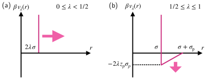
Figure 3: Visual representation of the evolution of $\beta v_{\lambda}(r)$ in (a) $0\leq\lambda<1/2$ given by Eq. (42) and (b) $1/2\leq\lambda\leq 1$ given by Eq. (43).

III.2.1 FRG

We consider the flow equations up to the second order, i.e., Eqs. (26), (28), and (II.5) for $m=2$. KSA (Eqs. (23) and (II.4)) is applied to the higher-order correlation functions $y^{(3)}_{\lambda}(r_{1},r_{2})$ and $y^{(4)}_{\lambda}(r_{1},r_{2},r_{3})$ appearing in the flow equations. We set the evolution in two steps: In the first step, the hard repulsive part of the interaction is taken with the RG-inspired flow represented in Eq. (34). We find that the application of the RG-inspired flow to the attractive part sometimes makes the numerical calculation unstable, which may be because the exponential factor $e^{-\beta v_{\lambda}(r)}$ can take a large value when $\beta v_{\lambda}(r)<0$ and the evolution becomes unexpectedly rapid during the RG-inspired flow. Instead of this, as the second step, we incorporate the attractive part with the adiabatic-connection-like flow. In summary, $\beta v_{\lambda}(r)$ is set as follows:

$$\beta v_{\lambda}(r)=\begin{cases}\infty&|r|<2\lambda\sigma\\ 0&|r|\geq 2\lambda\sigma\end{cases},$$ (42)

for $0\leq\lambda<1/2$, and

$$\beta v_{\lambda}(r)=\begin{cases}\infty&|r|<\sigma\\ -(2\lambda-1)z_{\rm p}(\sigma+\sigma_{\rm p}-|r|)&\sigma\leq|r|<\sigma+\sigma_{\rm p}\\ 0&\sigma+\sigma_{\rm p}\leq|r|\end{cases},$$ (43)

for $1/2\leq\lambda\leq 1$. This choice for $\beta v_{\lambda}(r)$ is visualized in Fig. 3. Since the interaction is turned off at $\lambda=0$, the initial condition required for solving the flow equations is given by $y^{(2)}_{\lambda=0}(r)=1$.

For the numerical implementation of our calculation, the GNU scientific library (GSL) is employed. In both the first and second parts of the evolution, i.e. $0\leq\lambda<1/2$ and $1/2\leq\lambda\leq 1$, respectively, the flow equations are solved with the eighth-order Runge–Kutta method within 20 steps. The cavity distribution function $y^{(2)}_{\lambda}(r)$ is derived on 512 grid points in $0\leq r<10\sigma$. To evaluate the spatial integral, we employ the Gauss–Krnord 21-point method with applying the spline interpolation for $y^{(2)}_{\lambda}(r)$.

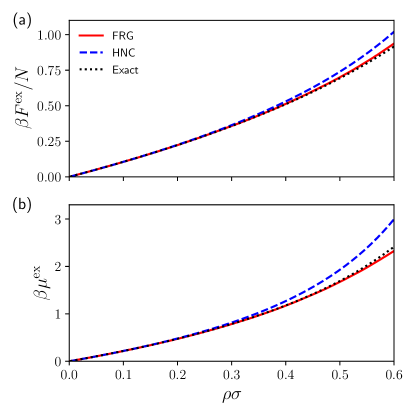
Figure 4: (a) Excess free energy per particle $\beta F^{\rm ex}/N$ and (b) chemical potential $\beta\mu^{\rm ex}$ of pure hard rods as functions of the packing fraction $\rho\sigma$. The results given by FRG, HNC, and exact solution are depicted by the red solid, blue dashed, and black dotted lines, respectively. PY results are not explicitly shown since they are identical to the exact solutions.

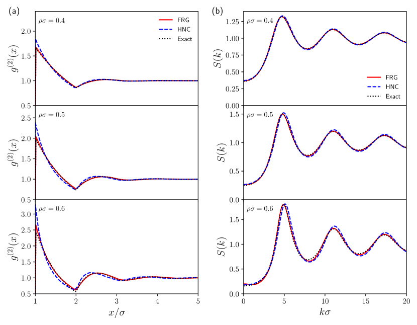
Figure 5: (a) Pair correlation functions $g^{(2)}(x)$ and (b) static structure functions $S(k)$ of pure hard rods calculated in $\rho\sigma=0.4$, $0.5$, and $0.6$. The style and color of each line corresponding to each method is the same as Fig. 4.

III.2.2 Integral-equation method

For the purpose of comparing our method to other conventional ones, we perform calculations by use of the integral-equation method with HNC and PY. In this method, the pair distribution function is calculated through the coupled integral equations composed of the OZ equation

$$h(r)=c(r)+\rho\int dr^{\prime}c(r-r^{\prime})h(r^{\prime})$$ (44)

and a closure relation, which is given by

$$h(r) =e^{-\beta v(r)+h(r)-c(r)}-1 (\text{HNC}),$$ (45)

$$h(r) =e^{-\beta v(r)}\left[1+h(r)-c(r)\right]-1 (\text{PY}).$$ (46)

Here, $c(r)$ is the direct correlation function and $h(r)=g^{(2)}(r)-1$ is the total correlation function. The coupled integral equations are solved numerically in an iterative manner. We use the exact solutions as the starting conditions of the iteration. From the resultant $g^{(2)}(r)$, we calculate $\beta P$ through the pressure equation:

$$\frac{\beta P}{\rho}=1-\rho\int_{0}^{\infty}dr\,r\frac{d\beta v(r)}{dr}g^{(2)}(r).$$ (47)

In the case of HNC, the excess chemical potential $\mu^{\rm ex}$ can be calculated using Hansen and McDonald (2013)

$$\beta\mu^{\rm ex}=\frac{1}{2}\rho\int drh(r)\left[h(r)-c(r)\right]-\rho\int drc(r).$$ (48)

In the case of PY, we calculate $\beta P(\rho)$ for various densities and perform the numerical integration with respect to $\rho$ to obtain the free-energy per particle:

$$\frac{\beta F}{N}=\int_{0}^{\infty}d\rho^{\prime}\frac{\beta P(\rho^{\prime})}{\rho^{\prime 2}},$$ (49)

which is derived from the thermodynamic relation:

$$P=-\left(\frac{\partial F}{\partial V}\right)_{\beta,N},$$ (50)

with the spatial volume $V$. The chemical potential is also obtained from

$$\beta\mu=\frac{F}{N}+\frac{\beta P}{\rho}.$$ (51)

III.3 Results for pure hard rods

We first show the case of a liquid composed of pure hard rods (Tonks gas), i.e., the case of $z_{\rm p}=0$. As for the thermodynamic quantities, the excess free energy per particle $F^{\rm ex}/N=F_{\lambda=1}/N-F_{\lambda=0}/N$ and the excess chemical potential $\mu^{\rm ex}=(\overline{\psi}_{\max,\lambda=1}-\overline{\psi}_{\max,\lambda=0})/\beta$ are obtained from FRG. Figure 4 shows the results of $\beta F^{\rm ex}/N$ and $\beta\mu^{\rm ex}$ together with the exact solutions and those obtained by HNC as functions of the packing fraction $\rho\sigma$. For the pure hard-rod system, PY gives the exact solutions Wertheim (1964); Verlet (1964). On the other hand, the results by HNC deviates from the exact solutions as the system becomes dense. In both results of $\beta F^{\rm ex}/N$ and $\beta\mu^{\rm ex}$, FRG shows more accurate results than those given by HNC.

Figure 5 shows the results of the pair distribution function $g^{(2)}(r)$ and the static structure factor $S(k)$ for some packing fractions. Through the numerical evaluation of the Fourier transform

$$g^{(2)}(r)=\frac{1}{\rho}\int_{-\infty}^{\infty}\frac{dk}{2\pi}e^{ikr}\left[S(k)-1\right]+1,$$ (52)

$g^{(2)}(r)$ is calculated from $S(k)$ in the case of the exact solution and vice versa in the cases of FRG and the integral-equation method. HNC misses the height of the first peak and the position of the second peak of $g^{(2)}(r)$, which becomes worse as the system becomes dense. In comparison to HNC, FRG gives more accurate results, although it slightly overestimates the height of the first peak at high density. FRG also gives more accurate results for the height and position of each peak of $S(k)$ than HNC. We also calculate the pressure from $F^{\rm ex}/N$ and $\beta\mu^{\rm ex}$ via Eq. (51). The result of the pressure by FRG is accurate as well as $F^{\rm ex}/N$ and $\beta\mu^{\rm ex}$.

III.4 Results for hard rod with attractive force

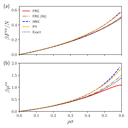
Figure 6: (a) Excess free energy per particle $\beta F^{\rm ex}/N$ and (b) chemical potential $\beta\mu^{\rm ex}$ in the case of $z_{\rm p}=1$ and $\sigma_{\rm s}=0.9$ as functions of the packing fraction $\rho\sigma$. The result of the fitting of $\beta F^{\rm ex}/N$ given by FRG with a fourth-order polynomial and the chemical potential calculated from the fitting function are shown as a gray dotted–dashed line. The PY results are shown as the orange long-dashed lines. For other methods, the style and color of each line corresponding to each method is the same as Fig. 4.

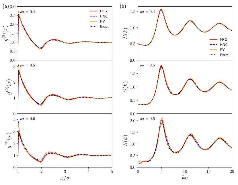
Figure 7: (a) Pair correlation functions $g^{(2)}(x)$ and (b) static structure functions $S(k)$ of hard rods with $z_{\rm p}=1$ and $\sigma_{\rm s}=0.9$ calculated in $\rho\sigma=0.4$, $0.5$, and $0.6$. The style and color of each line corresponding to each method is the same as Fig. 6.

We set $z_{p}=1$ and $\sigma_{p}=0.9$ to see the effect of the attractive force. The results for the thermodynamic quantities are shown in Fig. 6. The results of HNC is not shown in $\rho\sigma\geq 0.59$ since the calculation does not converge in this region. Due to the presence of the attractive force, the results of PY no longer agree with the exact solutions. It is noteworthy that FRG gives an accurate result for $\beta F^{\rm ex}/N$ in comparison to HNC and PY although PY has advantages for hard-rod systems as it gives exact solutions without the attractive force. On the other hand, an anomalous decrease is found near $\rho\sigma=0.6$ in the result of $\beta\mu^{\rm ex}$ by solving the FRG flow equation for the chemical potential (28). The pressure obtained from Eq. (51) also shows such a qualitative failure. The failure in contrast to the $\beta F^{\rm ex}/N$ may be because the flow equation for $\overline{\psi}_{\max,\lambda}$ is directly approximated with KSA as shown in Eq. (28) while the flow equation for $\beta F_{\lambda}/N$ is affected by the approximation indirectly through $y^{(2)}_{\lambda}(r)$ as shown in Eq. (26). Actually, the accuracy for $\beta\mu^{\rm ex}$ can differ from that for $\beta F^{\rm ex}_{\lambda}/N$ since our approximation violates the thermodynamic relation between $\beta\mu^{\rm ex}$ and $\beta F^{\rm ex}_{\lambda}/N$:

$$\beta\mu^{\rm ex}=\left(\frac{\partial\beta F^{\rm ex}}{\partial N}\right)_{\beta,V}=\frac{\beta F^{\rm ex}}{N}+\rho\left(\frac{\partial}{\partial\rho}\frac{\beta F^{\rm ex}}{N}\right)_{\beta}.$$ (53)

Instead of the flow equation for $\overline{\psi}_{\max,\lambda}$, we also evaluate $\beta\mu^{\rm ex}$ from this thermodynamic relation with evaluating the derivative of $\beta F^{\rm ex}_{\lambda}/N$ with respect to $\rho$. We fit the result of $\beta F^{\rm ex}/N$ by a fourth-order polynomial $\beta F^{\rm ex}/N=\sum_{i=1}^{4}a_{i}(\rho\sigma)^{i}$ and calculate the derivative from the fitting function, instead of performing the numerical derivative, which gives noisy results. The resultant fitting curve for $\beta F^{\rm ex}/N$ and $\beta\mu^{\rm ex}$ obtained by use of the fitting function are depicted as a gray dotted–dashed lines in Fig. 6. The result of $\beta\mu^{\rm ex}$ from the fitting-aided method gives reasonable and more accurate result than other methods.

Finally, the results for $g^{(2)}(r)$ and $S(k)$ are presented. Figure 7 shows the results of $g^{(2)}(r)$ and $S(k)$ calculated for some packing fractions. Particularly, FRG accurately predicts the height of the first peak, while other methods overestimate it as the system becomes dense. For $S(k)$, FRG gives results comparably accurate to PY, while there appears anomalous behavior near $k=0$ at high density.

IV Conclusion

In this paper, we present a method for classical liquids based on the functional renormalization group (FRG). The flow equations associated with the evolution of the two-body interaction are derived for the cavity distribution functions at arbitrary order, which are suitable to treat the short-range repulsion in the interaction. As a practical prescription for numerical calculations, we have proposed truncation method using the Kirkwood superposition approximation (KSA) and pointed out that choosing the evolution so that the interaction is gradually incorporated from the short-range to long-range parts is a suitable choice of the flow to treat a strong repulsive part with KSA. To illustrate how our method works, an application to a one-dimensional liquid composed of hard rods with and without an attractive force, which is an exactly solvable model, and the comparison to the integral-equation method based on the Ornstein-Zernike equation such as the hypernetted chain (HNC) and the Percus-Yevick (PY) equation have been presented. The flow equations up to the second order with KSA have been employed in the calculation. It is noteworthy that the excess free energy per particle and the height of the first peak of the pair distribution function $g^{(2)}(r)$ given by FRG show better results than those given by PY in the presence of the attractive force although PY has advantages for hard rods as it gives exact solutions without the attractive force. In comparison with HNC, FRG shows better results for the excess free energy per particle and the heights and positions of peaks in both cases with and without the attractive force. These results suggest that FRG can become an accurate framework to incorporate the repulsive and attractive parts of the interaction on the same footing without a reference system representing the contribution from short-range repulsion.

To further improve the accuracy and avoid anomalous behaviors of the excess chemical potential and structure functions in low momentum observed in our calculation in high density, the improvement of the approximation is desirable. In addition to treating higher-order flow equations, we have referred to a way to taking correction terms to KSA proposed in Ref. Abe (1959) into account. Meanwhile, one may alternatively be based on small expansion parameters realized by using the gradient expansion, HRT, or the Blaizot–Méndez–Wschebor approximation Blaizot et al. (2006) as discussed in Ref. Dupuis et al. (2021). Although we have treated the short-range repulsion by introducing the cavity distribution functions, one may alternatively use the method developed for spin systems Machado and Dupuis (2010), where the short-range fluctuations are incorporated by solving single site problems and FRG is used to incorporate longer-range fluctuations.

Our method can be straightforwardly extended to three-dimensional systems and applied to other potentials such as the Lennard–Jones potential, which are, of course, important future tasks. Regarding the calculation in three-dimensional systems, we believe that it is efficiently doable with employing efficient ways to evaluate the spatial integrals Barker and Monaghan (1962). The description of phase transition and the analysis of critical points, to which previous studies with FRG for classical liquids are devoted, is another topic of interest.

Appendix A Derivation of Eqs. (16) and (II.2)

In this Appendix, we present the derivation of Eqs. (16) and (II.2). For convenience, let us introduce the following notation for $m$-particle density, in which the argument is explicitly shown:

$$\rho^{(m)}_{\lambda}[\rho_{\rm v}]({\bf r}_{1},\ldots,{\bf r}_{m})= \left\langle\prod_{i=1}^{m}\left(\hat{\rho}({\bf r}_{i})-\sum_{j=1}^{i-1}\delta({\bf r}_{j}-{\bf r}_{i})\right)\right\rangle_{\lambda,\overline{\psi}_{\max,\lambda}[\rho_{\rm v}]}.$$ (54)

From Eqs. (11), (12), and (54), we have

$$\left(\frac{\delta^{2}\beta F_{\lambda}}{\delta\rho_{\rm v}\delta\rho_{\rm v}}\right)^{-1}[\rho_{\rm v}]({\bf r},{\bf r}^{\prime})= \left\langle\hat{\rho}({\bf r})\hat{\rho}({\bf r}^{\prime})\right\rangle_{\lambda,\overline{\psi}_{\max,\lambda}[\rho_{\rm v}]}-\rho_{\rm v}({\bf r})\rho_{\rm v}({\bf r}^{\prime})$$

$$= \rho^{(2)}_{\lambda}[\rho_{\rm v}]({\bf r},{\bf r}^{\prime})+\rho_{\rm v}({\bf r})\delta({\bf r}-{\bf r}^{\prime})-\rho_{\rm v}({\bf r})\rho_{\rm v}({\bf r}^{\prime}).$$ (55)

Inserting this into Eq. (6) with the substitution $\rho_{\rm v}({\bf r})=\rho({\bf r})$, we arrive at Eq. (16).

The derivation of Eq. (II.2) is based on the mathematical induction. In terms of $\rho^{(m)}_{\lambda}[\rho_{\rm v}]({\bf r}_{1},\ldots,{\bf r}_{m})$, Eq. (II.2) corresponds to the following equation:

$$\partial_{\lambda}\rho_{\lambda}^{(k)}[\rho_{\rm v}]({\bf r}_{1},\ldots,{\bf r}_{k})+\sum_{i<j}^{k}\partial_{\lambda}\left[\beta v_{\lambda}({\bf r}_{i}-{\bf r}_{j})\right]\rho_{\lambda}^{(k)}[\rho_{\rm v}]({\bf r}_{1},\ldots,{\bf r}_{k})$$

$$\quad=\int_{{\bf r}}\left[\rho^{(k+1)}_{\lambda}[\rho_{\rm v}]({\bf r}_{1},\ldots,{\bf r}_{k},{\bf r})-\rho_{\rm v}({\bf r})\rho^{(k)}_{\lambda}[\rho_{\rm v}]({\bf r}_{1},\ldots,{\bf r}_{k})\right]\partial_{\lambda}\overline{\psi}_{\max,\lambda}[\rho_{\rm v}]({\bf r})$$

$$\qquad+\rho^{(m)}_{\lambda}[\rho_{\rm v}]({\bf r}_{1},\ldots,{\bf r}_{k})\sum_{i=1}^{k}\partial_{\lambda}\overline{\psi}_{\max,\lambda}[\rho_{\rm v}]({\bf r}_{i})-\int_{{\bf r}}\sum_{i=1}^{k}\partial_{\lambda}\left[\beta v_{\lambda}({\bf r}-{\bf r}_{i})\right]\rho^{(k+1)}_{\lambda}[\rho_{\rm v}]({\bf r},{\bf r}_{1},\ldots,{\bf r}_{m})$$

$$\qquad-\frac{1}{2}\int_{{\bf r},{\bf r}^{\prime}}\partial_{\lambda}\left[\beta v_{\lambda}({\bf r}-{\bf r}^{\prime})\right]\left[\rho^{(k+2)}_{\lambda}[\rho_{\rm v}]({\bf r},{\bf r}^{\prime},{\bf r}_{1},\ldots,{\bf r}_{m})-\rho^{(2)}_{\lambda}[\rho_{\rm v}]({\bf r},{\bf r}^{\prime})\rho^{(k)}_{\lambda}[\rho_{\rm v}]({\bf r}_{1},\ldots,{\bf r}_{k})\right].$$ (56)

Let us show this equation holds for arbitrary integer $k\geq 1$.

For the proof, we prepare an expression for the derivative of $\rho^{(m)}_{\lambda}[\rho_{\rm v}]({\bf r}_{1},\ldots,{\bf r}_{m})$ with respect to $\rho_{\rm v}({\bf r})$:

$$\frac{\delta\rho^{(m)}_{\lambda}[\rho_{\rm v}]({\bf r}_{1},\ldots,{\bf r}_{m})}{\delta\rho_{\rm v}({\bf r})}= \left.\int_{{\bf r}_{m+1}}\frac{\delta\overline{\psi}_{\max,\lambda}[\rho_{\rm v}]({\bf r}_{m+1})}{\delta\rho_{\rm v}({\bf r})}\frac{\delta\rho^{(m)}_{\lambda}[\rho_{\rm v}]({\bf r}_{1},\ldots,{\bf r}_{m})}{\delta\overline{\psi}({\bf r}_{m+1})}\right|_{\overline{\psi}=\overline{\psi}_{\max,\lambda}[\rho_{\rm v}]}$$

$$= \left.\int_{{\bf r}_{m+1}}\frac{\delta^{2}\beta F_{\lambda}[\rho_{\rm v}]}{\delta\rho_{\rm v}({\bf r})\delta\rho_{\rm v}({\bf r}_{m+1})}\frac{\delta\rho^{(m)}_{\lambda}[\rho_{\rm v}]({\bf r}_{1},\ldots,{\bf r}_{m})}{\delta\overline{\psi}({\bf r}_{m+1})}\right|_{\overline{\psi}=\overline{\psi}_{\max,\lambda}[\rho_{\rm v}]},$$ (57)

where we have used Eq. (5). Using Eq. (15) and remembering Eq. (9), we have

$$\left.\frac{\delta\rho^{(m)}_{\lambda}[\rho_{\rm v}]({\bf r}_{1},\cdots,{\bf r}_{m})}{\delta\overline{\psi}({\bf r}_{m+1})}\right|_{\overline{\psi}=\overline{\psi}_{\max,\lambda}[\rho_{\rm v}]}$$

$$= \left\langle\hat{\rho}({\bf r}_{m+1})\prod_{i=1}^{m}\left(\hat{\rho}({\bf r}_{i})-\sum_{j=1}^{i-1}\delta({\bf r}_{j}-{\bf r}_{i})\right)\right\rangle_{\lambda,\overline{\psi}_{\max,\lambda}[\rho_{\rm v}]}-\rho({\bf r}_{m+1})\rho^{(m)}_{\lambda}[\rho_{\rm v}]({\bf r}_{1},\cdots,{\bf r}_{m})$$

$$= \rho^{(m+1)}_{\lambda}[\rho_{\rm v}]({\bf r}_{1},\cdots,{\bf r}_{m+1})+\rho^{(m)}_{\lambda}[\rho_{\rm v}]({\bf r}_{1},\cdots,{\bf r}_{m})\left[\sum_{k=1}^{m}\delta({\bf r}_{k}-{\bf r}_{m+1})-\rho_{\rm v}({\bf r}_{m+1})\right].$$ (58)

Therefore, Eq. (A) is rewritten as

$$\frac{\delta\rho^{(m)}_{\lambda}[\rho_{\rm v}]({\bf r}_{1},\ldots,{\bf r}_{m})}{\delta\rho_{\rm v}({\bf r})}$$

$$= \int_{{\bf r}^{\prime}}\frac{\delta^{2}\beta F_{\lambda}[\rho_{\rm v}]}{\delta\rho_{\rm v}({\bf r})\delta\rho_{\rm v}({\bf r}^{\prime})}\left(\rho^{(m+1)}_{\lambda}[\rho_{\rm v}]({\bf r}_{1},\cdots,{\bf r}_{m},{\bf r}^{\prime})+\rho^{(m)}_{\lambda}[\rho_{\rm v}]({\bf r}_{1},\cdots,{\bf r}_{m})\left[\sum_{k=1}^{m}\delta({\bf r}_{k}-{\bf r}^{\prime})-\rho_{\rm v}({\bf r}^{\prime})\right]\right).$$ (59)

Equation (A) for $k=1$ is obtained from the first derivative of Eq. (6):

$$\partial_{\lambda}\frac{\delta\beta F_{\lambda}[\rho_{\rm v}]}{\delta\rho_{\rm v}({\bf r}_{1})}= \frac{1}{2}\int_{{\bf r},{\bf r}^{\prime}}\partial_{\lambda}\beta v_{\lambda}({\bf r}-{\bf r}^{\prime})\frac{\delta}{\delta\rho_{\rm v}({\bf r}_{1})}\left(\rho_{\rm v}({\bf r})\rho_{\rm v}({\bf r}^{\prime})+\left(\frac{\delta^{2}\beta F_{\lambda}}{\delta\rho_{\rm v}\delta\rho_{\rm v}}\right)^{-1}[\rho_{\rm v}]({\bf r},{\bf r}^{\prime})-\rho_{\rm v}({\bf r})\delta({\bf r}-{\bf r}^{\prime})\right).$$ (60)

From Eqs. (A) and (A), we obtain

$$\frac{\delta}{\delta\rho_{\rm v}({\bf r}_{1})}\left[\rho_{\rm v}({\bf r})\rho_{\rm v}({\bf r}^{\prime})+\left(\frac{\delta^{2}\beta F_{\lambda}}{\delta\rho_{\rm v}\delta\rho_{\rm v}}\right)^{-1}[\rho_{\rm v}]({\bf r},{\bf r}^{\prime})-\rho_{\rm v}({\bf r})\delta({\bf r}-{\bf r}^{\prime})\right]$$

$$= \int_{{\bf r}^{\prime\prime}}\frac{\delta^{2}\beta F_{\lambda}[\rho_{\rm v}]}{\delta\rho_{\rm v}({\bf r}_{1})\delta\rho_{\rm v}({\bf r}^{\prime\prime})}\left(\rho^{(3)}_{\lambda}[\rho_{\rm v}]({\bf r},{\bf r}^{\prime},{\bf r}^{\prime\prime})+\rho^{(2)}_{\lambda}[\rho_{\rm v}]({\bf r},{\bf r}^{\prime})\left[\sum_{k=1}^{m}\delta({\bf r}-{\bf r}^{\prime\prime})+\delta({\bf r}^{\prime}-{\bf r}^{\prime\prime})-\rho_{\rm v}({\bf r}^{\prime\prime})\right]\right).$$ (61)

By use of this relation and Eq. (5), Eq. (60) is rewritten as follows:

$$\partial_{\lambda}\overline{\psi}_{\max,\lambda}[\rho_{\rm v}]({\bf r}_{1})$$

$$= \frac{1}{2}\int_{{\bf r},{\bf r}^{\prime}}\partial_{\lambda}\beta v_{\lambda}({\bf r}-{\bf r}^{\prime})$$

$$\times\int_{{\bf r}^{\prime\prime}}\frac{\delta^{2}\beta F_{\lambda}[\rho_{\rm v}]}{\delta\rho_{\rm v}({\bf r}_{1})\delta\rho_{\rm v}({\bf r}^{\prime\prime})}\left(\rho^{(3)}_{\lambda}[\rho_{\rm v}]({\bf r},{\bf r}^{\prime},{\bf r}^{\prime\prime})+\rho^{(2)}_{\lambda}[\rho_{\rm v}]({\bf r},{\bf r}^{\prime})\left[\sum_{k=1}^{m}\delta({\bf r}-{\bf r}^{\prime\prime})+\delta({\bf r}^{\prime}-{\bf r}^{\prime\prime})-\rho_{\rm v}({\bf r}^{\prime\prime})\right]\right).$$ (62)

Multiplying the inverse of the second derivative of $\beta F_{\lambda}[\rho_{\rm v}]$ and using Eq. (A), we have

$$0= \int_{{\bf r}}\left[\rho^{(2)}_{\lambda}[\rho_{\rm v}]({\bf r}_{1},{\bf r})-\rho_{\rm v}({\bf r})\rho_{\rm v}({\bf r}_{1})\right]\partial_{\lambda}\overline{\psi}_{\max,\lambda}[\rho_{\rm v}]({\bf r})+\rho_{\rm v}({\bf r}_{1})\partial_{\lambda}\overline{\psi}_{\max,\lambda}[\rho_{\rm v}]({\bf r}_{1})$$

$$-\int_{{\bf r}}\partial_{\lambda}\left[\beta v_{\lambda}({\bf r}-{\bf r}_{i})\right]\rho^{(2)}_{\lambda}[\rho_{\rm v}]({\bf r},{\bf r}_{1})-\frac{1}{2}\int_{{\bf r},{\bf r}^{\prime}}\partial_{\lambda}\left[\beta v_{\lambda}({\bf r}-{\bf r}^{\prime})\right]\left[\rho^{(3)}_{\lambda}[\rho_{\rm v}]({\bf r},{\bf r}^{\prime},{\bf r}_{1})-\rho_{\rm v}({\bf r}_{1})\rho^{(2)}_{\lambda}[\rho_{\rm v}]({\bf r},{\bf r}^{\prime})\right].$$ (63)

This equation corresponds to Eq. (A) for $k=1$.

Now we assume that Eq. (A) holds for all $k\leq m$ and show that this equation also holds for $k=m+1$ by differentiating Eq. (A) for $k=m$. As one can see from Eq. (A), there appears $\partial_{\lambda}\delta^{2}\beta F_{\lambda}[\rho_{\rm v}]/\delta\rho_{\rm v}({\bf r})\delta\rho_{\rm v}({\bf r}^{\prime})$ from the $\rho_{\rm v}$-derivative of the first term in the left-hand side of Eq. (A). Such a factor also appears from the $\rho_{\rm v}$-derivative of $\overline{\psi}_{\max,\lambda}[\rho_{\rm v}]({\bf r})$ as one can see from Eq. (5). These terms involving the factor $\partial_{\lambda}\delta^{2}\beta F_{\lambda}[\rho_{\rm v}]/\delta\rho_{\rm v}({\bf r})\delta\rho_{\rm v}({\bf r}^{\prime})$ cancel each other. Then the $\rho_{\rm v}$-derivative of Eq. (A) for $k=m$ reads

$$\int_{{\bf r}^{\prime}}\frac{\delta^{2}\beta F_{\lambda}[\rho_{\rm v}]}{\delta\rho_{\rm v}({\bf r}^{\prime\prime})\delta\rho_{\rm v}({\bf r}^{\prime})}\left(\partial_{\lambda}\rho^{(m+1)}_{\lambda}[\rho_{\rm v}]({\bf r}_{1},\cdots,{\bf r}_{m},{\bf r}^{\prime})+\partial_{\lambda}\rho^{(m)}_{\lambda}[\rho_{\rm v}]({\bf r}_{1},\cdots,{\bf r}_{m})\left[\sum_{k=1}^{m}\delta({\bf r}_{k}-{\bf r}^{\prime})-\rho_{\rm v}({\bf r}^{\prime})\right]\right)$$

$$+\sum_{i<j}^{m}\partial_{\lambda}\left[\beta v_{\lambda}({\bf r}_{i}-{\bf r}_{j})\right]\frac{\delta}{\delta\rho_{\rm v}({\bf r}^{\prime\prime})}\rho_{\lambda}^{(m)}[\rho_{\rm v}]({\bf r}_{1},\ldots,{\bf r}_{m})$$

$$= \int_{{\bf r}}\left[\frac{\delta}{\delta\rho_{\rm v}({\bf r}^{\prime\prime})}\rho^{(m+1)}_{\lambda}[\rho_{\rm v}]({\bf r}_{1},\ldots,{\bf r}_{m},{\bf r})-\rho_{\rm v}({\bf r})\frac{\delta}{\delta\rho_{\rm v}({\bf r}^{\prime\prime})}\rho^{(m)}_{\lambda}[\rho_{\rm v}]({\bf r}_{1},\ldots,{\bf r}_{m})\right]\partial_{\lambda}\overline{\psi}_{\max,\lambda}[\rho_{\rm v}]({\bf r})$$

$$-\rho^{(m)}_{\lambda}[\rho_{\rm v}]({\bf r}_{1},\ldots,{\bf r}_{m})\partial_{\lambda}\overline{\psi}_{\max,\lambda}[\rho_{\rm v}]({\bf r}^{\prime\prime})+\frac{\delta}{\delta\rho_{\rm v}({\bf r}^{\prime\prime})}\rho^{(m)}_{\lambda}[\rho_{\rm v}]({\bf r}_{1},\ldots,{\bf r}_{m})\sum_{i=1}^{m}\partial_{\lambda}\overline{\psi}_{\max,\lambda}[\rho_{\rm v}]({\bf r}_{i})$$

$$-\int_{{\bf r}}\sum_{i=1}^{m}\partial_{\lambda}\left[\beta v_{\lambda}({\bf r}-{\bf r}_{i})\right]\frac{\delta}{\delta\rho_{\rm v}({\bf r}^{\prime\prime})}\rho^{(m+1)}_{\lambda}[\rho_{\rm v}]({\bf r},{\bf r}_{1},\ldots,{\bf r}_{m})$$

$$-\frac{1}{2}\int_{{\bf r},{\bf r}^{\prime}}\partial_{\lambda}\left[\beta v_{\lambda}({\bf r}-{\bf r}^{\prime})\right]\left[\frac{\delta}{\delta\rho_{\rm v}({\bf r}^{\prime\prime})}\rho^{(m+2)}_{\lambda}[\rho_{\rm v}]({\bf r},{\bf r}^{\prime},{\bf r}_{1},\ldots,{\bf r}_{m})-\rho^{(2)}_{\lambda}[\rho_{\rm v}]({\bf r},{\bf r}^{\prime})\frac{\delta}{\delta\rho_{\rm v}({\bf r}^{\prime\prime})}\rho^{(m)}_{\lambda}[\rho_{\rm v}]({\bf r}_{1},\ldots,{\bf r}_{m})\right]$$

$$+\frac{1}{2}\int_{{\bf r},{\bf r}^{\prime}}\partial_{\lambda}\left[\beta v_{\lambda}({\bf r}-{\bf r}^{\prime})\right]\rho^{(m)}_{\lambda}[\rho_{\rm v}]({\bf r}_{1},\ldots,{\bf r}_{m})\frac{\delta}{\delta\rho_{\rm v}({\bf r}^{\prime\prime})}\rho^{(2)}_{\lambda}[\rho_{\rm v}]({\bf r},{\bf r}^{\prime}).$$ (64)

Multiplying $\left(\delta^{2}\beta F_{\lambda}/\delta\rho_{\rm v}\delta\rho_{\rm v}\right)^{-1}[\rho_{\rm v}]$, we have

$$\partial_{\lambda}\rho^{(m+1)}_{\lambda}[\rho_{\rm v}]({\bf r}_{1},\cdots,{\bf r}_{m+1})+\partial_{\lambda}\rho^{(m)}_{\lambda}[\rho_{\rm v}]({\bf r}_{1},\cdots,{\bf r}_{m})\left[\sum_{k=1}^{m}\delta({\bf r}_{k}-{\bf r}^{\prime})-\rho({\bf r}_{m+1})\right]$$

$$+\sum_{i<j}^{m}\partial_{\lambda}\left[\beta v_{\lambda}({\bf r}_{i}-{\bf r}_{j})\right]R_{\lambda}^{(m)}[\rho_{\rm v}]({\bf r}_{1},\ldots,{\bf r}_{m};{\bf r}_{m+1})$$

$$= \int_{{\bf r}}\left[R_{\lambda}^{(m+1)}[\rho_{\rm v}]({\bf r}_{1},\ldots,{\bf r}_{m},{\bf r};{\bf r}_{m+1})-\rho_{\rm v}({\bf r})R_{\lambda}^{(m)}[\rho_{\rm v}]({\bf r}_{1},\ldots,{\bf r}_{m};{\bf r}_{m+1})\right]\partial_{\lambda}\overline{\psi}_{\max,\lambda}[\rho_{\rm v}]({\bf r})$$

$$-\int_{{\bf r}}\left(\frac{\delta^{2}\beta F_{\lambda}}{\delta\rho_{\rm v}\delta\rho_{\rm v}}\right)^{-1}[\rho_{\rm v}]({\bf r}_{m+1},{\bf r})\rho^{(m)}_{\lambda}[\rho_{\rm v}]({\bf r}_{1},\ldots,{\bf r}_{m})\partial_{\lambda}\overline{\psi}_{\max,\lambda}[\rho_{\rm v}]({\bf r})$$

$$+R_{\lambda}^{(m)}[\rho_{\rm v}]({\bf r}_{1},\ldots,{\bf r}_{m};{\bf r}_{m+1})\sum_{i=1}^{m}\partial_{\lambda}\overline{\psi}_{\max,\lambda}[\rho_{\rm v}]({\bf r}_{i})$$

$$-\int_{{\bf r}}\sum_{i=1}^{m}\partial_{\lambda}\left[\beta v_{\lambda}({\bf r}-{\bf r}_{i})\right]R_{\lambda}^{(m+1)}[\rho_{\rm v}]({\bf r}_{1},\ldots,{\bf r}_{m},{\bf r};{\bf r}_{m+1})$$

$$-\frac{1}{2}\int_{{\bf r},{\bf r}^{\prime}}\partial_{\lambda}\left[\beta v_{\lambda}({\bf r}-{\bf r}^{\prime})\right]\left[R_{\lambda}^{(m+2)}[\rho_{\rm v}]({\bf r}_{1},\ldots,{\bf r}_{m},{\bf r},{\bf r}^{\prime};{\bf r}_{m+1})-\rho^{(2)}_{\lambda}[\rho_{\rm v}]({\bf r},{\bf r}^{\prime})R_{\lambda}^{(m)}[\rho_{\rm v}]({\bf r}_{1},\ldots,{\bf r}_{m};{\bf r}_{m+1})\right]$$

$$+\frac{1}{2}\int_{{\bf r},{\bf r}^{\prime}}\partial_{\lambda}\left[\beta v_{\lambda}({\bf r}-{\bf r}^{\prime})\right]\rho^{(m)}_{\lambda}[\rho_{\rm v}]({\bf r}_{1},\ldots,{\bf r}_{m})R_{\lambda}^{(2)}[\rho_{\rm v}]({\bf r},{\bf r}^{\prime};{\bf r}_{m+1}).$$ (65)

Here, $R_{\lambda}^{(m)}[\rho_{\rm v}]({\bf r}_{1},\ldots,{\bf r}_{m};{\bf r}_{m+1})$ is defined by

$$R_{\lambda}^{(m)}[\rho_{\rm v}]({\bf r}_{1},\ldots,{\bf r}_{m};{\bf r})=\int_{{\bf r}^{\prime}}\left(\frac{\delta^{2}\beta F_{\lambda}}{\delta\rho_{\rm v}\delta\rho_{\rm v}}\right)^{-1}[\rho_{\rm v}]({\bf r},{\bf r}^{\prime})\frac{\delta}{\delta\rho_{\rm v}({\bf r}^{\prime})}\rho_{\lambda}^{(m)}[\rho_{\rm v}]({\bf r}_{1},\ldots,{\bf r}_{m}).$$

By use of Eq. (A), we get

$$R_{\lambda}^{(m)}[\rho_{\rm v}]({\bf r}_{1},\ldots,{\bf r}_{m};{\bf r}_{m+1})$$

$$\quad=\rho^{(m+1)}_{\lambda}[\rho_{\rm v}]({\bf r}_{1},\cdots,{\bf r}_{m+1})+\rho^{(m)}_{\lambda}[\rho_{\rm v}]({\bf r}_{1},\cdots,{\bf r}_{m})C({\bf r}_{1},\ldots,{\bf r}_{m};{\bf r}_{m+1}),$$ (66)

$$R_{\lambda}^{(m+1)}[\rho_{\rm v}]({\bf r}_{1},\ldots,{\bf r}_{m},{\bf r};{\bf r}_{m+1})$$

$$\quad=\rho^{(m+2)}_{\lambda}[\rho_{\rm v}]({\bf r}_{1},\cdots,{\bf r}_{m+1},{\bf r})+\rho^{(m+1)}_{\lambda}[\rho_{\rm v}]({\bf r}_{1},\cdots,{\bf r}_{m},{\bf r})\left[\delta({\bf r}-{\bf r}_{m+1})+C({\bf r}_{1},\ldots,{\bf r}_{m};{\bf r}_{m+1})\right],$$ (67)

$$R_{\lambda}^{(m+2)}[\rho_{\rm v}]({\bf r}_{1},\ldots,{\bf r}_{m},{\bf r},{\bf r}^{\prime};{\bf r}_{m+1})$$

$$\quad=\rho^{(m+3)}_{\lambda}[\rho_{\rm v}]({\bf r}_{1},\cdots,{\bf r}_{m+1},{\bf r},{\bf r}^{\prime})$$

$$\qquad+\rho^{(m+2)}_{\lambda}[\rho_{\rm v}]({\bf r}_{1},\cdots,{\bf r}_{m},{\bf r},{\bf r}^{\prime})\left[\delta({\bf r}-{\bf r}_{m+1})+\delta({\bf r}^{\prime}-{\bf r}_{m+1})+C({\bf r}_{1},\ldots,{\bf r}_{m};{\bf r}_{m+1})\right],$$ (68)

with

$$C({\bf r}_{1},\ldots,{\bf r}_{m};{\bf r}_{m+1})=\sum_{k=1}^{m}\delta({\bf r}_{k}-{\bf r}_{m+1})-\rho_{\rm v}({\bf r}_{m+1}).$$ (69)

Using this relation and Eq. (A), we find the terms involving the factor $C({\bf r}_{1},\ldots,{\bf r}_{m};{\bf r}_{m+1})$ cancel each other. Then Eq. (A) is rewritten as follows:

$$\partial_{\lambda}\rho^{(m+1)}_{\lambda}[\rho_{\rm v}]({\bf r}_{1},\cdots,{\bf r}_{m+1})+\sum_{i<j}^{m}\partial_{\lambda}\left[\beta v_{\lambda}({\bf r}_{i}-{\bf r}_{j})\right]\rho_{\lambda}^{(m+1)}[\rho_{\rm v}]({\bf r}_{1},\ldots,{\bf r}_{m+1})$$

$$= \int_{{\bf r}}\left[\rho_{\lambda}^{(m+2)}[\rho_{\rm v}]({\bf r}_{1},\ldots,{\bf r}_{m+1},{\bf r})-\rho_{\rm v}({\bf r})\rho_{\lambda}^{(m+1)}[\rho_{\rm v}]({\bf r}_{1},\ldots,{\bf r}_{m+1})\right]\partial_{\lambda}\overline{\psi}_{\max,\lambda}[\rho_{\rm v}]({\bf r})$$

$$-\int_{{\bf r}}\left(\frac{\delta^{2}\beta F_{\lambda}}{\delta\rho_{\rm v}\delta\rho_{\rm v}}\right)^{-1}[\rho_{\rm v}]({\bf r}_{m+1},{\bf r})\rho^{(m)}_{\lambda}[\rho_{\rm v}]({\bf r}_{1},\ldots,{\bf r}_{m})\partial_{\lambda}\overline{\psi}_{\max,\lambda}[\rho_{\rm v}]({\bf r})$$

$$+\rho_{\lambda}^{(m+1)}[\rho_{\rm v}]({\bf r}_{1},\ldots,{\bf r}_{m+1})\sum_{i=1}^{m+1}\partial_{\lambda}\overline{\psi}_{\max,\lambda}[\rho_{\rm v}]({\bf r}_{i})$$

$$-\int_{{\bf r}}\sum_{i=1}^{m}\partial_{\lambda}\left[\beta v_{\lambda}({\bf r}-{\bf r}_{i})\right]\rho_{\lambda}^{(m+2)}[\rho_{\rm v}]({\bf r}_{1},\ldots,{\bf r}_{m+1},{\bf r})-\sum_{i=1}^{m}\partial_{\lambda}\left[\beta v_{\lambda}({\bf r}_{m+1}-{\bf r}_{i})\right]\rho_{\lambda}^{(m+1)}[\rho_{\rm v}]({\bf r}_{1},\ldots,{\bf r}_{m+1})$$

$$-\frac{1}{2}\int_{{\bf r},{\bf r}^{\prime}}\partial_{\lambda}\left[\beta v_{\lambda}({\bf r}-{\bf r}^{\prime})\right]\left[\rho_{\lambda}^{(m+3)}[\rho_{\rm v}]({\bf r}_{1},\ldots,{\bf r}_{m+1},{\bf r},{\bf r}^{\prime})-\rho^{(2)}_{\lambda}[\rho_{\rm v}]({\bf r},{\bf r}^{\prime})\rho_{\lambda}^{(m+1)}[\rho_{\rm v}]({\bf r}_{1},\ldots,{\bf r}_{m+1})\right]$$

$$-\int_{{\bf r}}\partial_{\lambda}\left[\beta v_{\lambda}({\bf r}-{\bf r}_{m+1})\right]\rho_{\lambda}^{(m+2)}[\rho_{\rm v}]({\bf r}_{1},\ldots,{\bf r}_{m+1},{\bf r})$$

$$+\frac{1}{2}\int_{{\bf r},{\bf r}^{\prime}}\partial_{\lambda}\left[\beta v_{\lambda}({\bf r}-{\bf r}^{\prime})\right]\rho^{(m)}_{\lambda}[\rho_{\rm v}]({\bf r}_{1},\ldots,{\bf r}_{m})$$

$$\times\left[\rho^{(3)}_{\lambda}[\rho_{\rm v}]({\bf r},{\bf r}^{\prime},{\bf r}_{m+1})+\rho^{(2)}_{\lambda}[\rho_{\rm v}]({\bf r},{\bf r}^{\prime})\left(\delta({\bf r}-{\bf r}_{m+1})+\delta({\bf r}^{\prime}-{\bf r}_{m+1})-\rho_{\rm v}({\bf r}_{m+1})\right)\right].$$ (70)

By use of Eqs. (A) and (A), one finds that the second and last terms in the right-hand side of Eq. (A) cancel each other. Finally, we can rewrite Eq. (A) to obtain Eq. (A) for $k=m+1$. Therefore, it is proved that Eq. (A) holds for arbitrary $k\geq 1$. By inserting $\rho_{\rm v}({\bf r})=\rho({\bf r})$, Eq. (II.2) is obtained.

References

- Hansen and McDonald (2013) J. Hansen and I. McDonald, Theory of Simple Liquids: with Applications to Soft Matter (Elsevier Science, 2013).
- Barker and Henderson (1976) J. A. Barker and D. Henderson, Rev. Mod. Phys. 48, 587 (1976).
- Kirkwood et al. (1950) J. G. Kirkwood, E. K. Maun, and B. J. Alder, The Journal of Chemical Physics 18, 1040 (1950).
- Levesque (1966) D. Levesque, Physica 32, 1985 (1966).
- Parola and Reatto (1985) A. Parola and L. Reatto, Phys. Rev. A 31, 3309 (1985).
- Parola et al. (1993) A. Parola, D. Pini, and L. Reatto, Phys. Rev. E 48, 3321 (1993).
- Parola and Reatto (1995) A. Parola and L. Reatto, Advances in Physics 44, 211 (1995).
- Parola et al. (2008) A. Parola, D. Pini, and L. Reatto, Phys. Rev. Lett. 100, 165704 (2008).
- Parola et al. (2009) A. Parola, D. Pini, and L. Reatto, Molecular Physics 107, 503 (2009).
- Parola and Reatto (2012) A. Parola and L. Reatto, Molecular Physics 110, 2859 (2012).
- Salvino and White (1992) L. W. Salvino and J. A. White, The Journal of Chemical Physics 96, 4559 (1992).
- White and Zhang (1993) J. A. White and S. Zhang, The Journal of Chemical Physics 99, 2012 (1993).
- White and Zhang (1995) J. A. White and S. Zhang, The Journal of Chemical Physics 103, 1922 (1995).
- Iso and Kawana (2019) S. Iso and K. Kawana, Prog. Theor. Exp. Phys. 2019, 013A01 (2019), arXiv:1808.08133 [cond-mat.stat-mech] .
- Caillol (2006) J.-M. Caillol, Molecular Physics 104, 1931 (2006).
- Caillol (2011) J.-M. Caillol, Molecular Physics 109, 2813 (2011).
- (17) L. Lue, AIChE Journal 61, 2985.
- Wegner and Houghton (1973) F. J. Wegner and A. Houghton, Phys. Rev. A 8, 401 (1973).
- Wilson and Kogut (1974) K. G. Wilson and J. Kogut, Phys. Rep. 12, 75 (1974).
- Polchinski (1984) J. Polchinski, Nucl. Phys. B 231, 269 (1984).
- Wetterich (1993) C. Wetterich, Phys. Lett. B 301, 90 (1993).
- Berges et al. (2002) J. Berges, N. Tetradis, and C. Wetterich, Phys. Rep. 363, 223 (2002).
- Pawlowski (2007) J. M. Pawlowski, Ann. Phys. 322, 2831 (2007).
- Metzner et al. (2012) W. Metzner, M. Salmhofer, C. Honerkamp, V. Meden, and K. Schönhammer, Rev. Mod. Phys. 84, 299 (2012).
- Dupuis et al. (2021) N. Dupuis, L. Canet, A. Eichhorn, W. Metzner, J. Pawlowski, M. Tissier, and N. Wschebor, Physics Reports (2021), https://doi.org/10.1016/j.physrep.2021.01.001.
- Polonyi and Sailer (2002) J. Polonyi and K. Sailer, Phys. Rev. B 66, 155113 (2002).
- Schwenk and Polonyi (2004) A. Schwenk and J. Polonyi, in 32nd International Workshop on Gross Properties of Nuclei and Nuclear Excitation: Probing Nuclei and Nucleons with Electrons and Photons (Hirschegg 2004) Hirschegg, Austria, January 11-17, 2004 (2004) pp. 273–282, arXiv:nucl-th/0403011 .
- Kemler and Braun (2013) S. Kemler and J. Braun, J. Phys. G 40, 085105 (2013).
- Rentrop et al. (2015) J. F. Rentrop, S. G. Jakobs, and V. Meden, Journal of Physics A: Mathematical and Theoretical 48, 145002 (2015).
- Kemler et al. (2017) S. Kemler, M. Pospiech, and J. Braun, J. Phys. G 44, 015101 (2017).
- Liang et al. (2018) H. Liang, Y. Niu, and T. Hatsuda, Phys. Lett. B 779, 436 (2018).
- Yokota et al. (2019a) T. Yokota, K. Yoshida, and T. Kunihiro, Phys. Rev. C 99, 024302 (2019a).
- Yokota et al. (2019b) T. Yokota, K. Yoshida, and T. Kunihiro, Prog. Theor. Exp. Phys. 2019, 011D01 (2019b).
- Yokota and Naito (2019) T. Yokota and T. Naito, Phys. Rev. B 99, 115106 (2019).
- Yokota and Naito (2021) T. Yokota and T. Naito, Phys. Rev. Research 3, L012015 (2021).
- Yokota et al. (2020) T. Yokota, H. Kasuya, K. Yoshida, and T. Kunihiro, Prog. Theor. Exp. Phys. 2021, 013A03 (2020).
- Sumi et al. (2016) T. Sumi, Y. Maruyama, A. Mitsutake, and K. Koga, The Journal of Chemical Physics 144, 224104 (2016), https://doi.org/10.1063/1.4953191 .
- Meeron and Siegert (1968) E. Meeron and A. J. F. Siegert, The Journal of Chemical Physics 48, 3139 (1968), https://doi.org/10.1063/1.1669587 .
- GROUBA et al. (2004) V. D. GROUBA, A. V. ZORIN, and L. A. SEVASTIANOV, International Journal of Modern Physics B 18, 1 (2004).
- Abe (1959) R. Abe, Progress of Theoretical Physics 21, 421 (1959).
- Ichimaru (1970) S. Ichimaru, Phys. Rev. A 2, 494 (1970).
- Canet et al. (2003) L. Canet, B. Delamotte, D. Mouhanna, and J. Vidal, Phys. Rev. D 67, 065004 (2003).
- Archer et al. (2017) A. J. Archer, B. Chacko, and R. Evans, The Journal of Chemical Physics 147, 034501 (2017).
- Brader and Evans (2002) J. Brader and R. Evans, Physica A: Statistical Mechanics and its Applications 306, 287 (2002), invited Papers from the 21th IUPAP International Conference on St atistical Physics.
- Percus (1982) J. K. Percus, Journal of Statistical Physics 28, 67 (1982).
- Wertheim (1964) M. S. Wertheim, Journal of Mathematical Physics 5, 643 (1964).
- Verlet (1964) L. Verlet, Physica 30, 95 (1964).
- Blaizot et al. (2006) J.-P. Blaizot, R. Méndez-Galain, and N. Wschebor, Physics Letters B 632, 571 (2006).
- Machado and Dupuis (2010) T. Machado and N. Dupuis, Phys. Rev. E 82, 041128 (2010).
- Barker and Monaghan (1962) J. A. Barker and J. J. Monaghan, The Journal of Chemical Physics 36, 2564 (1962).