A Powerful Subvector Anderson-Rubin Test in Linear Instrumental Variables Regression with Conditional Heteroskedasticity

Abstract

We introduce a new test for a two-sided hypothesis involving a subset of the structural parameter vector in the linear instrumental variables (IVs) model. Guggenberger et al. (2019), GKM19 from now on, introduce a subvector Anderson-Rubin (AR) test with data-dependent critical values that has asymptotic size equal to nominal size for a parameter space that allows for arbitrary strength or weakness of the IVs and has uniformly nonsmaller power than the projected AR test studied in Guggenberger et al. (2012). However, GKM19 imposes the restrictive assumption of conditional homoskedasticity. The main contribution here is to robustify the procedure in GKM19 to arbitrary forms of conditional heteroskedasticity. We first adapt the method in GKM19 to a setup where a certain covariance matrix has an approximate Kronecker product (AKP) structure which nests conditional homoskedasticity. The new test equals this adaption when the data is consistent with AKP structure as decided by a model selection procedure. Otherwise the test equals the AR/AR test in Andrews (2017) that is fully robust to conditional heteroskedasticity but less powerful than the adapted method. We show theoretically that the new test has asymptotic size bounded by the nominal size and document improved power relative to the AR/AR test in a wide array of Monte Carlo simulations when the covariance matrix is not too far from AKP.

Keywords: Asymptotic size, conditional heteroskedasticity, Kronecker product, linear IV regression, subvector inference, weak instruments

JEL codes: C12, C26

1 Introduction

Robust and powerful subvector inference constitutes an important problem in Econometrics. For instance, it is standard practice to report confidence intervals on each of the coefficients in a linear regression model. By robust we mean a testing procedure for a hypothesis of (or a confidence region for) a subset of the structural parameter vector such that the asymptotic size is bounded by the nominal size for a parameter space that allows for weak or partial identification. Recent contributions to robust subvector inference have been made in the context of the linear instrumental variables (IVs from now on) model (see, for example, Dufour and Taamouti (2005), Guggenberger et al. (2012) (GKMC from now on), Guggenberger et al. (2019) (GKM19 from now on), and Kleibergen (2021)), GMM models (see, for example, Chaudhuri and Zivot (2011), Andrews and Cheng (2014), Andrews and Mikusheva (2016), Andrews (2017), and Han and McCloskey (2019)), and also models defined by moment (in)equalities (see, for example, Bugni et al. (2017), Gafarov (2017), and Kaido et al. (2019)). GKM19 introduce a new subvector test that compares the AR subvector statistic to conditional critical values that adapt to the strength or weakness of identification and verify that the resulting test has correct asymptotic size for a parameter space that imposes conditional homoskedasticity (CHOM from now on) and uniformly improves on the power of the projected AR test studied in Dufour and Taamouti (2005).

The contribution of the current paper is to provide a robust subvector test that improves the power of another robust subvector test by combining it with a more powerful test that is robust for only a smaller parameter space. More specifically, in the context of the linear IV model, we first provide a modification of the subvector AR test of GKM19, called the AR_AKP,α test, where $\alpha$ denotes the nominal size. We verify that it has correct asymptotic size for a parameter space that nests the setup with CHOM and also allows for particular cases of conditional heteroskedasticity (CHET from now on), namely setups where a particular covariance matrix has a Kronecker product (KP from now on) structure. For example, the data generating process (DGP from now on) has a KP structure if the vector of structural and reduced-form errors equals a random vector independent of the IVs times a scalar function of the IVs. In particular then, the variances of all the errors depend on the IVs by the same multiplicative constant given as a scalar function of the IVs. In the companion paper Guggenberger et al. (2022) (GKM22 from now on) we find that KP structure is not rejected at the 5% nominal size in more than 63% of empirical data sets we studied of several recently published empirical papers (namely, 38 of 60 specifications are not rejected; and, including cases with clustering, 56 out of 118 are not rejected). For comparison, CHOM is rejected for 57 of the 60 specifications considered at the 5% nominal size, using the test in Kelejian (1982). Of course, these findings do not prove that empirical data sets do have KP structure as the low number of rejections of KP structure may be due to type II errors of the test. However, coupled with the quite favorable finite sample power results of the test of KP structure reported in GKM22 (for sample sizes of $n=200$) we believe that KP structure might be compatible with a sizable subset of empirical data sets.

Second, depending on a model selection mechanism that determines whether the data are compatible with KP, the recommended test then equals the AR_AKP,α test or the AR/AR test in Andrews (2017) that is robust to arbitrary forms of CHET. We show that the recommended test has correct asymptotic size. An important ingredient in establishing that is showing that the AR_AKP,α test does not reject less often under the null hypothesis than the AR/AR test when the data are close to KP structure.

We propose two different model selection methods. One is based on the KPST test statistic introduced in GKM22 for testing the null hypothesis that a covariance matrix has KP structure. The other one is based on the standardized norm of the distance between the covariance matrix estimator and its closest KP approximation. As in the model selection method proposed in Andrews and Soares (2010), we compare the test statistic to a user chosen threshold that, in the asymptotics, is let go to infinity. The thresholds can be chosen differently depending on the number of IVs $k$ and parameters not under test. Based on comprehensive finite sample simulations we provide choices for the thresholds for several values of $k$ that lead to good control of the finite sample size.

As the main contribution of the paper, we verify that the resulting test, called $\varphi_{MS-AKP,\alpha}$ test, has asymptotic size bounded by the nominal size $\alpha$ under certain conditions on the selection mechanism and implementation of the AR/AR test at nominal size $\alpha-\delta$ for some arbitrarily small $\delta>0$.

In a Monte Carlo study, we compare the suggested new test $\varphi_{MS-AKP,\alpha}$ with several alternatives given in Andrews (2017), in particular, the AR/AR and the AR/QLR1 tests. Andrews (2017) fills a very important gap in the literature on subvector inference by providing two-step Bonferroni-like methods for a rich class of models that nests GMM, that i) control the asymptotic size under relatively mild high-level conditions that allow for CHET, ii) are asymptotically non-conservative (in contrast to standard Bonferroni methods) and iii) for the case of AR/QLR1 is asymptotically efficient under strong identification (while the AR/AR test is not asymptotically efficient under strong identification in overidentified situations). In contrast, the test considered here, $\varphi_{MS-AKP,\alpha}$, can only be used in the linear IV model and is not asymptotically efficient under strong identification. The Monte Carlo study finds that $\varphi_{MS-AKP,\alpha}$ has uniformly higher rejection probabilities than the AR/AR test for all the DGPs considered. That includes the null rejection probabilities (NRPs from now on) with the $\varphi_{MS-AKP,\alpha}$ test having finite sample size of 6% versus the 5.4% of the AR/AR test at nominal size 5%. Based on the Monte Carlo study we conclude that relative to the AR/QLR1 test, $\varphi_{MS-AKP,\alpha}$ can be a useful alternative in terms of power in situations of weak or mixed identification strengths when the degree of overidentification is small and the covariance matrix of the data is not too far from KP structure. Whenever the data are compatible with KP structure, it also offers an important computational advantage because the AR_AKP,α test is given in closed form. In contrast, implementation of the two-step Bonferroni-like methods require minimization of a statistic over a set that has dimension equal to the number of parameters not under test. The computation time should grow exponentially in the dimension of that set which constitutes a computational challenge especially when an applied researcher uses the proposed methods for the construction of a confidence region by test inversion. This being said, an applied researcher who uses the $\varphi_{MS-AKP,\alpha}$ test has to be ready to implement the AR/AR test in case it is determined that KP structure is not compatible with the data. Given the construction of the AR_AKP,α test it is not surprising to find the relative best performance of the $\varphi_{MS-AKP,\alpha}$ test to occur under weak identification. Namely, the critical values of the former test adapt to the strength of identification and can be substantially lower than the corresponding chi-square critical values when identification is deemed to be weak.

The rest of the paper is organized as follows. In Section 2 we introduce a version of a subvector Anderson and Rubin (1949) test that has correct asymptotic size for a parameter space that imposes an approximate Kronecker product (AKP) structure for the covariance matrix. In Section 3 we introduce the new test that has correct asymptotic size for a parameter space that does not impose any structure on the covariance matrix and therefore, in particular, allows for arbitrary forms of conditional heteroskedasticity. Finally, in Section 4 we study the finite sample properties of the test. Proofs are given in the Appendix at the end.

Notation: Throughout the paper, we denote by “$\otimes$” the KP of two matrices, by $vec(\cdot)$ the column vectorization of a matrix, and by $||\cdot||$ the Frobenius norm. We use the notation $M_{A}:=I_{n}-P_{A}$ and $P_{A}:=A(A^{\prime}A)^{-1}A^{\prime}$ for any full rank matrix $A\in\Re^{n\times k}.$

2 Subvector AR Test under Approximate Kronecker Product Structure

Assume the linear IV model is given by the equations

$$y =Y\beta+W\gamma+\varepsilon$$

$$Y =\overline{Z}\Pi_{Y}+V_{Y}$$

$$W =\overline{Z}\Pi_{W}+V_{W},$$ (2.1)

where $y\in\Re^{n},$ $Y\in\Re^{n\times m_{Y}},$ $W\in\Re^{n\times m_{W}},$ and $\overline{Z}\in\Re^{n\times k}.$ Here, $W$ contains endogenous regressors, while the regressors $Y$ may be endogenous or exogenous. We assume that $k-m_{W}\geq 1$ and $m_{W}\geq 1.$ The reduced form can be written as

$$\left(\begin{array}[c]{ccc}y&Y&W\end{array}\right)=\overline{Z}\left(\begin{array}[c]{cc}\Pi_{Y}&\Pi_{W}\end{array}\right)\left(\begin{array}[c]{ccc}\beta&I_{m_{Y}}&0^{m_{Y}\times m_{W}}\\ \gamma&0^{m_{W}\times m_{Y}}&I_{m_{W}}\end{array}\right)+\underbrace{\left(\begin{array}[c]{ccc}v_{y}&V_{Y}&V_{W}\end{array}\right)}_{V},$$ (2.2)

where $v_{y}:=V_{Y}\beta+$ $V_{W}\gamma+\varepsilon$ (which depends on the true $\beta$ and $\gamma),$ $V_{W}^{\prime}=(V_{W,1},\ldots,V_{W,n}),$ $V_{Y}^{\prime}=(V_{Y,1},\ldots,V_{Y,n}),$ $\overline{Z}^{\prime}=(\overline{Z}_{1},\ldots,\overline{Z}_{n}).$ By $V_{i},$ for $i=1,...,n,$ we denote the $i$-th row of $V$ written as a column vector and similarly for other matrices.

The objective is to test the subvector hypothesis

$$H_{0}:\beta=\beta_{0}\text{ against\ }H_{1}:\beta\neq\beta_{0},$$ (2.3)

using tests whose size, i.e. the highest NRP over a large class of distributions for $(\varepsilon_{i},\overline{Z}_{i}^{\prime},V_{Y,i}^{\prime},V_{W,i}^{\prime})$ and the unrestricted nuisance parameters $\Pi_{Y},$ $\Pi_{W},$ and $\gamma$, equals the nominal size $\alpha$, at least asymptotically. In particular, weak identification and non-identification of $\beta$ and $\gamma$ are allowed for. The setup allows testing the coefficients of exogenous or endogenous regressors $Y$ in the presence of endogenous regressors $W$. We impose the following assumption as in GKM19 (from where the name of the assumption is inherited).

Assumption B: The random vectors $(\varepsilon_{i},\overline{Z}_{i}^{\prime},V_{Y,i}^{\prime},V_{W,i}^{\prime})$ for $i=1,...,n$ in (2.1) are i.i.d. with distribution $F.$

For a given sequence $a_{n}=o(1)$ in $\Re_{\geq 0},$ we define a sequence of parameter spaces $\mathcal{F}_{AKP,a_{n}}$ for $(\gamma,\Pi_{W},\Pi_{Y},F)$ under the null hypothesis $H_{0}:\beta=\beta_{0}$ that is larger than the corresponding ones in GKMC and GKM19 in that general forms of AKP structures for the variance matrix

$$\overline{R}_{F}:=E_{F}(vec(\overline{Z}_{i}U_{i}^{\prime})(vec(\overline{Z}_{i}U_{i}^{\prime}))^{\prime})\in\Re^{kp\times kp}$$ (2.4)

are allowed for. Namely, for $U_{i}:=(\varepsilon_{i}+V_{W,i}^{\prime}\gamma,V_{W,i}^{\prime})^{\prime}$ (which equals $(v_{yi}-V_{Y,i}^{\prime}\beta,V_{W,i}^{\prime})^{\prime}$), $p:=1+m_{W},$ and $m:=m_{Y}+m_{W}$ let

$$\mathcal{F}_{AKP,a_{n}} =\{(\gamma,\Pi_{W},\Pi_{Y},F):\gamma\overset{}{\in}\Re^{m_{W}},\Pi_{W}\overset{}{\in}\Re^{k\times m_{W}},\Pi_{Y}\overset{}{\in}\Re^{k\times m_{Y}},$$

$$\text{ }E_{F}(||T_{i}||^{2+\delta_{1}})\overset{}{\leq}B,\text{ for }T_{i}\overset{}{\in}\{vec(\overline{Z}_{i}U_{i}^{\prime}),||\overline{Z}_{i}||^{2}\},$$

$$E_{F}(\overline{Z}_{i}V_{i}^{\prime})\overset{}{=}0^{k\times(m+1)},\text{ }\overline{R}_{F}\overset{}{=}G_{F}\otimes\overline{H}_{F}+\Upsilon_{n},\text{ }$$

$$\kappa_{\min}(A)\overset{}{\geq}\delta_{2}\text{ for }A\overset{}{\in}\{E_{F}(\overline{Z}_{i}^{\prime}\overline{Z}_{i}),G_{F},\overline{H}_{F}\}\}$$ (2.5)

for symmetric matrices $\Upsilon_{n}\in\Re^{kp\times kp}$ such that

$$||\Upsilon_{n}||\leq a_{n},$$ (2.6)

positive definite (pd from now on) symmetric matrices $G_{F}\in\Re^{p\times p}$ (whose upper left element is normalized to 1) and $\overline{H}_{F}\in\Re^{k\times k},$ $\delta_{1},\delta_{2}>0,$ $B<\infty$. Note that the factors in the KP $G_{F}\otimes\overline{H}_{F}$ are not uniquely defined due to the summand $\Upsilon_{n}$. Note that no restriction is imposed on the variance matrix of $vec(\overline{Z}_{i}V_{Y,i}^{\prime})$ and, in particular, $E_{F}(vec(\overline{Z}_{i}V_{Y,i}^{\prime})(vec(\overline{Z}_{i}V_{Y,i}^{\prime}))^{\prime})$ does not need to factor into a KP.

The factorization of the covariance matrix into an AKP in line three of (2.5) is a weaker assumption than CHOM. Under CHOM, we have $G_{F}=E_{F}\left(U_{i}U_{i}^{\prime}\right)$ and $\overline{H}_{F}=E_{F}(\overline{Z}_{i}^{\prime}\overline{Z}_{i})$ (prior to the normalization of the upper left element of $G_{F}$) and $\Upsilon_{n}=0^{kp\times kp}.$ The AKP structure allowed for here (but not in GKMC and GKM19) also covers some important cases of CHET involving $vec(\overline{Z}_{i}U_{i}^{\prime})$.

Examples. i) Consider the case in (2.1) where $(\widetilde{\varepsilon}_{i},\widetilde{V}_{W,i}^{\prime})^{\prime}\in\Re^{p}$ are i.i.d. zero mean with a pd variance matrix, independent of $\overline{Z}_{i},$ and $(\varepsilon_{i},V_{W,i}^{\prime})^{\prime}:=f(\overline{Z}_{i})(\widetilde{\varepsilon}_{i},\widetilde{V}_{W,i}^{\prime})^{\prime}$ for some scalar valued function $f$ of $\overline{Z}_{i}.$ In that case, the covariance matrix $\overline{R}_{F}$ can be written

$$E_{F}(vec(\overline{Z}_{i}U_{i}^{\prime})(vec(\overline{Z}_{i}U_{i}^{\prime}))^{\prime})$$

$$=E_{F}\left(U_{i}U_{i}^{\prime}\otimes\overline{Z}_{i}\overline{Z}_{i}^{\prime}\right)$$

$$=E_{F}\left((\varepsilon_{i}+V_{W,i}^{\prime}\gamma,V_{W,i}^{\prime})^{\prime}(\varepsilon_{i}+V_{W,i}^{\prime}\gamma,V_{W,i}^{\prime})\otimes\overline{Z}_{i}\overline{Z}_{i}^{\prime}\right)$$

$$=E_{F}\left((\widetilde{\varepsilon}_{i}+\widetilde{V}_{W,i}^{\prime}\gamma,\widetilde{V}_{W,i}^{\prime})^{\prime}(\widetilde{\varepsilon}_{i}+\widetilde{V}_{W,i}^{\prime}\gamma,\widetilde{V}_{W,i}^{\prime})\right)\otimes E_{F}\left(f(\overline{Z}_{i})^{2}\overline{Z}_{i}\overline{Z}_{i}^{\prime}\right)$$ (2.7)

and thus has KP structure even though, obviously, CHOM is not satisfied because

$$E_{F}(U_{i}U_{i}^{\prime}|\overline{Z}_{i})=f(\overline{Z}_{i})^{2}E_{F}(\widetilde{\varepsilon}_{i}+\widetilde{V}_{W,i}^{\prime}\gamma,\widetilde{V}_{W,i}^{\prime})^{\prime}(\widetilde{\varepsilon}_{i}+\widetilde{V}_{W,i}^{\prime}\gamma,\widetilde{V}_{W,i}^{\prime})$$ (2.8)

depends on $\overline{Z}_{i}.$

We can construct illustrative examples where the proportionality $(\varepsilon_{i},V_{W,i}^{\prime})^{\prime}:=f(\overline{Z}_{i})(\widetilde{\varepsilon}_{i},\widetilde{V}_{W,i}^{\prime})^{\prime}$ (that would imply KP structure) holds. Consider e.g. the model

$$y_{i} =Y_{i}\beta_{i}+W_{i}\gamma$$

$$W_{i} =Y_{i}\phi_{i}+X_{i}\Phi_{X}$$

where the covariates $Y_{i}$ and $X_{i}$ are exogenous, the variables $y_{i},W_{i}$ are endogenous, and $Y_{i}$ has heterogeneous causal effects on $y_{i},W_{i},$ denoted by $\beta_{i},\phi_{i},$ respectively. Let $\beta:=E\left(\beta_{i}\right),$ $\phi:=E\left(\phi_{i}\right),$ define $\widetilde{\varepsilon}_{i}:=\beta_{i}-\beta$ and $\widetilde{V}_{Wi}:=\phi_{i}-\phi,$ and assume that $\widetilde{\varepsilon}_{i},\widetilde{V}_{Wi}$ are orthogonal to $Z_{i}:=\left(Y_{i},X_{i}\right).$ Then, this fits exactly into the setup above with $f\left(Z_{i}\right)=Y_{i}.$ In other words, KP structure can result as a special case of heterogeneous causal effects.

ii) In a wage regression to assess the effect of ”years of education”, the assumption of CHOM would require that e.g. the variance of ”wage” does not depend on the included regressor ”race”. This assumption is incompatible with recent US data where the wage dispersion is largest for Asians. Instead, the construction $(\varepsilon_{i},V_{W,i}^{\prime})^{\prime}:=f(\overline{Z}_{i})(\widetilde{\varepsilon}_{i},\widetilde{V}_{W,i}^{\prime})^{\prime}$ in i) allows for dependence of the variances of the regressand and all endogenous regressors on a scalar function of $\overline{Z}_{i}.$ The maintained restriction is that all these variances are affected approximately by the same scalar function of $\overline{Z}_{i}.$ In the related paper, GKM22, we test the null hypothesis of KP structure for 118 specifications in about a dozen highly cited papers and find that at the 5% nominal size in 47.5% of the cases the null is not rejected.

In this section we will introduce a new conditional subvector AR_AKP test and show it has asymptotic size with respect to the parameter space $\mathcal{F}_{AKP,a_{n}}$ equal to the nominal size. We next define the new test statistic and the critical value for the case considered here of AKP structure.

Estimation of the two factors in the AKP structure: Define

$$Z_{i}:=(n^{-1}\overline{Z}^{\prime}\overline{Z})^{-1/2}\overline{Z}_{i}\in\Re^{k}$$ (2.9)

and $Z\in\Re^{n\times k}$ with rows given by $Z_{i}^{\prime}$ for $i=1,...,n.$ Define an estimator of the matrix

$$R_{F}=(I_{p}\otimes(E_{F}\overline{Z}_{i}\overline{Z}_{i}^{\prime})^{-1/2})\overline{R}_{F}(I_{p}\otimes(E_{F}\overline{Z}_{i}\overline{Z}_{i}^{\prime})^{-1/2})\in\Re^{kp\times kp}$$ (2.10)

by

$$\widehat{R}_{n} :=n^{-1}{\textstyle\sum\nolimits_{i=1}^{n}}f_{i}f_{i}^{\prime}\in\Re^{kp\times kp},\text{ where}$$

$$f_{i} :=((M_{Z}\overline{Y}_{0})_{i},(M_{Z}W)_{i}^{\prime})^{\prime}\otimes Z_{i}\in\Re^{kp},\text{ and }\overline{Y}_{0}:=y-Y\beta_{0}.$$ (2.11)

Note that $\widehat{R}_{n}$ is automatically a centered estimator because, as straightforward calculations show, $n^{-1}{\textstyle\sum\nolimits_{i}}f_{i}=0.$ From $\overline{R}_{F}=G_{F}\otimes\overline{H}_{F}+\Upsilon_{n},$ it follows that $R_{F}=G_{F}\otimes H_{F}+o(1)$ for

$$H_{F}:=(E_{F}\overline{Z}_{i}\overline{Z}_{i}^{\prime})^{-1/2}\overline{H}_{F}(E_{F}\overline{Z}_{i}\overline{Z}_{i}^{\prime})^{-1/2}.$$ (2.12)

Let

$$(\widehat{G}_{n},\widehat{H}_{n})=\arg\min||G\otimes H-\widehat{R}_{n}||,$$ (2.13)

where the minimum is taken over $(G,H)$ for $G\in\Re^{p}\times p,$ $H\in\Re^{k}\times k$ being pd, symmetric matrices, and normalized such that the upper left element of $G$ equals 1.

It can be shown that $(\widehat{G}_{n},\widehat{H}_{n})$ are given in closed form by the following construction. First, for a pd matrix $A\in\Re^{kp\times kp}$ define the rearrangement of $A$ as

$$\mathcal{R}(A) :=\left(\begin{array}[c]{c}A_{1}\\ ...\\ A_{p}\end{array}\right)\in\Re^{pp\times kk},\text{ where }$$ (2.17)

$$A_{j} :=\left(\begin{array}[c]{c}(vec(A_{1j}))^{\prime}\\ ...\\ (vec(A_{pj}))^{\prime}\end{array}\right)\in\Re^{p\times kk}\text{ for }j=1,...,p,$$ (2.21)

where $A_{lj}\in\Re^{k\times k}$ denotes the $(l,j)$ submatrix of dimensions $k\times k,$ where $l,j=1,...,p.$ Second, denote by

$$\widehat{L}^{\prime}\mathcal{R}(A)\widehat{N}=diag(\widehat{\sigma}_{l})\in\Re^{pp\times kk}$$ (2.22)

a singular value decomposition of $\mathcal{R}(A)$, where the singular values $\widehat{\sigma}_{l}$ for $l=1,...,p^{2}$ are ordered non-increasingly. Finally, denote by $\widehat{L}(:,1)$ and $\widehat{N}(:,1)$ singular vectors corresponding to the largest singular value $\widehat{\sigma}_{1}$ and let $\widehat{L}(1,1)$ denote the first component of $\widehat{L}(:,1).$ Then, letting the role of $A$ be played by $\widehat{R}_{n}$ in (2.22), minimizers $(\widehat{G}_{n},\widehat{H}_{n})$ to (2.13) are defined by

$$vec(\widehat{G}_{n})=\widehat{L}(:,1)/\widehat{L}(1,1)\text{ and }vec(\widehat{H}_{n})=\widehat{\sigma}_{1}\widehat{L}(1,1)\widehat{N}(:,1),$$ (2.23)

where $\widehat{L}(1,1)>0$ whenever $\widehat{R}_{n}$ is pd. By Lemma 4 below, the definition given in (2.23) is unique for all large enough $n$ wp1 and

$$\widehat{G}_{n}-G_{F_{n}}\rightarrow 0^{p\times p}\text{ and }\widehat{H}_{n}-H_{F_{n}}\rightarrow 0^{k\times k}\text{ a.s.}$$ (2.24)

under certain sequences $F_{n}$ as defined in $\mathcal{F}_{AKP,a_{n}}$ for which $R_{F_{n}}=G_{F_{n}}\otimes H_{F_{n}}+o(1)$ (where $R_{F_{n}}$ is defined in (2.10) with $F$ replaced by $F_{n}$), $H_{F_{n}}:=(E_{F_{n}}\overline{Z}_{i}\overline{Z}_{i}^{\prime})^{-1/2}\overline{H}_{F_{n}}(E_{F_{n}}\overline{Z}_{i}\overline{Z}_{i}^{\prime})^{-1/2}$ (as defined in (2.12)), and the upper left element of $G_{F_{n}}$ is normalized to 1.

Definition of the conditional subvector test: We denote the subvector AR statistic when the variance matrix has AKP structure by $AR_{AKP,n}(\beta_{0})$ and define it as the smallest root $\hat{\kappa}_{pn}$ of the roots $\hat{\kappa}_{in},$ $i=1,...,p$ (ordered nonincreasingly) of the characteristic polynomial

$$\left|\hat{\kappa}I_{p}-n^{-1}\widehat{G}_{n}^{-1/2}\left(\overline{Y}_{0},W\right)^{\prime}Z\widehat{H}_{n}^{-1}Z^{\prime}\left(\overline{Y}_{0},W\right)\widehat{G}_{n}^{-1/2}\right|=0.$$ (2.25)

The conditional subvector test AR_AKP,α rejects $H_{0}$ at nominal size $\alpha$ if

$$AR_{AKP,n}(\beta_{0})>c_{1-\alpha}(\hat{\kappa}_{1n},k-m_{W}),$$ (2.26)

where $c_{1-\alpha}\left(\cdot,\cdot\right)$ is defined as follows. Muirhead (1978), in the case where $m_{W}=1$ and assuming normality, provides an approximate, nuisance parameter free, conditional density of the smaller eigenvalue $\hat{\kappa}_{2n}$ given the larger one $\hat{\kappa}_{1n}$ for any degree of overidentification $k-m_{W},$ see (2.12) in GKM19 for the conditional pdf. For given $\hat{\kappa}_{1n}$ and arbitrary $m_{W},$ $c_{1-\alpha}(\hat{\kappa}_{1n},k-m_{W})$ denotes the $1-\alpha$-quantile of that approximation. GKM19 (Table 1 and Supplement C) provide $c_{1-\alpha}(\hat{\kappa}_{1n},k-m_{W})$ for $\alpha=1,5,10\%,$ $k-m_{W}=1,...,20$ and a fine grid of values for $\hat{\kappa}_{1n},$ say $\hat{\kappa}_{1,1}\leq...\leq\hat{\kappa}_{1,j}\leq...\leq\hat{\kappa}_{1,J}$ for some large $J.$ We reproduce Table 1 (that covers the case $\alpha=5\%$ and $k-m_{W}=4)$ from GKM19 below. Conditional critical values for values of $\hat{\kappa}_{1n}$ not reported in the tables are obtained by linear interpolation. Specifically, let $q_{1-\alpha,j}(k-1)$ denote the $1-\alpha$ quantile of the distribution whose density is given by (2.12) in GKM19 with $\hat{\kappa}_{1n}$ replaced by $\hat{\kappa}_{1,j}$. The end point of the grid $\hat{\kappa}_{1,J}$ should be chosen high enough so that $q_{1-\alpha,J}(k-m_{W})\approx\chi_{k-m_{W},1-\alpha}^{2}$. For any realization of $\hat{\kappa}_{1n}\leq\hat{\kappa}_{1,J}$, find $j$ such that $\hat{\kappa}_{1n}\in\left[\hat{\kappa}_{1,j-1},\hat{\kappa}_{1,j}\right]$ with $\hat{\kappa}_{1,0}=0$ and $q_{1-\alpha,0}\left(k-m_{W}\right)=0$, and let

$$c_{1-\alpha}\left(\hat{\kappa}_{1n},k-m_{W}\right):=\frac{\hat{\kappa}_{1,j}-\hat{\kappa}_{1n}}{\hat{\kappa}_{1,j}-\hat{\kappa}_{1,j-1}}q_{1-\alpha,j-1}\left(k-m_{W}\right)+\frac{\hat{\kappa}_{1n}-\hat{\kappa}_{1,j-1}}{\hat{\kappa}_{1,j}-\hat{\kappa}_{1,j-1}}q_{1-\alpha,j}\left(k-m_{W}\right).$$ (2.27)

Table 1: $cv=c_{1-\alpha}(\hat{\kappa}_{1},k-m_{W})$ for $\alpha=5\%,$ $k-m_{W}=4$ for various values of $\hat{\kappa}_{1}$

$\hat{\kappa}_{1}$	cv	$\hat{\kappa}_{1}$	cv	$\hat{\kappa}_{1}$	cv	$\hat{\kappa}_{1}$	cv	$\hat{\kappa}_{1}$	cv	$\hat{\kappa}_{1}$	cv	$\hat{\kappa}_{1}$	cv	$\hat{\kappa}_{1}$	cv	$\hat{\kappa}_{1}$	cv
1.2	1.1	2.1	1.9	3.2	2.9	4.5	3.9	5.9	4.9	7.4	5.9	9.4	6.9	12.5	7.9	20.9	8.9
1.3	1.2	2.3	2.1	3.5	3.1	4.7	4.1	6.2	5.1	7.8	6.1	9.9	7.1	13.4	8.1	26.5	9.1
1.4	1.3	2.5	2.3	3.7	3.3	5.0	4.3	6.5	5.3	8.2	6.3	10.5	7.3	14.5	8.3	39.9	9.3
1.6	1.5	2.7	2.5	4.0	3.5	5.3	4.5	6.8	5.5	8.6	6.5	11.1	7.5	15.9	8.5	57.4	9.4
1.8	1.7	3.0	2.7	4.2	3.7	5.6	4.7	7.1	5.7	9.0	6.7	11.7	7.7	17.9	8.7	1000	9.48

Denote by $P_{(\gamma,\Pi_{W},\Pi_{Y},F)}(\cdot)$ the probability of an event under the null hypothesis when the true values of the structural and reduced form parameters and the distribution of the random variables are given by $(\gamma,\Pi_{W},\Pi_{Y},F).$ Recall the definition of the parameter space $\mathcal{F}_{AKP,a_{n}}$ in (2.5). We can now formulate the main result of this section.

Theorem 1

Under Assumption B, the conditional subvector test AR_AKP,α defined in $($2.26$)$ implemented at nominal size $\alpha$ has asymptotic size, i.e.

$$\lim\sup_{n\rightarrow\infty}\sup_{(\gamma,\Pi_{W},\Pi_{Y},F)\in\mathcal{F}_{AKP,a_{n}}}P_{(\gamma,\Pi_{W},\Pi_{Y},F)}(AR_{AKP,n}(\beta_{0})>c_{1-\alpha}(\hat{\kappa}_{1n},k-m_{W}))$$

equal to $\alpha$ for $\alpha\in\left\{1\%,5\%,10\%\right\}$ and $k-m_{W}\in\left\{1,...,20\right\}.$

Comment. 1. The conditional subvector test AR_AKP,α adapts the test in GKM19 from a setup under CHOM to AKP structure. The modification involves replacing the matrices $\left(\overline{Y}_{0},W\right)^{\prime}M_{\overline{Z}}\allowbreak\left(\overline{Y}_{0},W\right)/(n-k)$ and $n^{-1}\overline{Z}^{\prime}\overline{Z}$ in GKM19 by the matrices $\widehat{G}_{n}$ and $\widehat{H}_{n},$ respectively, in (2.25) to account for the more general structure of the covariance matrix. Some portions of the proof follow similar steps as the proof of Theorem 5 in GKM19. In particular, one portion of the proof relies on a one-dimensional simulation exercise to prove that the NRPs are bounded by the nominal size. This exercise could be extended to choices of $\alpha$ and $k-m_{W}$ beyond those in the theorem and likely the theorem would extend to many more choices.

2. Trivially, under the same assumptions as in Theorem 1, we obtain that

$$\lim\sup_{n\rightarrow\infty}\sup_{(\gamma,\Pi_{W},\Pi_{Y},F)\in\mathcal{F}_{AKP,a_{n}}}P_{(\gamma,\Pi_{W},\Pi_{Y},F)}(AR_{AKP,n}(\beta_{0})>\chi_{k-m_{W},1-\alpha}^{2})=\alpha.$$

That is, the generalization of the subvector test in GKMC to AKP structure has correct asymptotic size. This result is obtained fully analytically; its proof does not require any simulations.

3. Invariance with respect to nonsingular transformations of the IV matrix. The identifying power of the model comes from the moment condition $E_{F}\varepsilon_{i}\overline{Z}_{i}=E_{F}(y_{i}-Y_{i}^{\prime}\beta-W_{i}^{\prime}\gamma)\overline{Z}_{i}=0.$ This moment condition obviously still holds when the instrument vector is premultiplied by a nonrandom nonsingular matrix $A\in\Re^{k\times k},$ i.e. $E_{F}\varepsilon_{i}A\overline{Z}_{i}=0.$ It then seems reasonable to look for testing procedures whose outcome is invariant to such nonsingular transformations. In the weak IV literature, e.g. Andrews et al. (2006) and Andrews et al. (2019) and references therein, the class of (similar) invariant tests to orthogonal transformations $A$, that is, changes of the coordinate system, has been studied. The transformation of the IVs in (2.9) is performed in order for the test to be invariant to nonsingular transformations of the IVs.

If the conditional subvector AR_AKP test defined in (2.26) (and $\widehat{R}_{n}$ in (2.11)) was defined with $\overline{Z}_{i}$ in place of $Z_{i}$ it would be invariant to orthogonal transformations but not necessarily to nonsingular ones. To see the former, denote by $\widehat{R}_{nA}$ the matrix $\widehat{R}_{n}$ when the instrument vector has been transformed to $A\overline{Z}_{i}$ (and consequently $\overline{Z}$ is changed to $\overline{Z}A^{\prime}).$ Then the claim follows from $\mathcal{R}(\widehat{R}_{nA})=\mathcal{R}(\widehat{R}_{n})(A^{\prime}\otimes A^{\prime})$ (which holds for any nonsingular matrix $A$ by straightforward calculations using $vec(ABC)=(C^{\prime}\otimes A)vec(B)$ for any conformable matrices $A,B,$ and $C$ and $M_{\overline{Z}}=M_{\overline{Z}A^{\prime}})$ which implies $\widehat{G}_{nA}=\widehat{G}_{n}$ and $\widehat{H}_{nA}=A\widehat{H}_{n}A^{\prime}$ when $A$ is orthogonal, where again $\widehat{G}_{nA}$ and $\widehat{H}_{nA}$ denote the matrices $\widehat{G}_{n}$ and $\widehat{H}_{n}$ when the instrument vector $\overline{Z}_{i}$ has been transformed to $A\overline{Z}_{i}$. It then follows that the matrix $n^{-1}\widehat{G}_{n}^{-1/2}\left(\overline{Y}_{0},W\right)^{\prime}\overline{Z}\widehat{H}_{n}^{-1}\overline{Z}^{\prime}\left(\overline{Y}_{0},W\right)\widehat{G}_{n}^{-1/2}$ in (2.25) (and thus its eigenvalues) remain invariant under orthogonal transformations $\overline{Z}_{i}\rightarrow A\overline{Z}_{i}$ of the instrument matrix. This test however is not invariant in general to arbitrary nonsingular transformations.

But with the replacement of $\overline{Z}_{i}$ by $Z_{i}$ as done in (2.11) and, correspondingly, $\overline{Z}$ by $\overline{Z}(n^{-1}\overline{Z}^{\prime}\overline{Z})^{-1/2}$ in (2.25), the test is invariant against nonsingular transformations $A$. The invariance of this test to arbitrary nonsingular transformations $\overline{Z}_{i}\rightarrow A\overline{Z}_{i}$ of the instrument matrix (which leads to a transformation of $Z_{i}$ to $(A\overline{Z}^{\prime}\overline{Z}A^{\prime})^{-1/2}A\overline{Z}_{i}$) follows from straightforward calculations and the fact that the matrix

$$T_{A}:=(\overline{Z}^{\prime}\overline{Z})^{1/2}A^{\prime}(A\overline{Z}^{\prime}\overline{Z}A^{\prime})^{-1/2}\in\Re^{k\times k}$$ (2.28)

is orthogonal. In particular, one can easily show that the matrices $\mathcal{R}(\widehat{R}_{n}),$ $\widehat{G}_{n},$ and $\widehat{H}_{n}$ that appear as ingredients in the conditional subvector test AR_AKP,α with $A=I_{k}$ are related to the corresponding matrices $\mathcal{R}(\widehat{R}_{nA}),$ $\widehat{G}_{nA},$ and $\widehat{H}_{nA}$, when $A$ is an arbitrary nonsingular matrix, via

$$\mathcal{R}(\widehat{R}_{nA})=\mathcal{R}(\widehat{R}_{n})\left(T_{A}\otimes T_{A}\right),\text{ }\widehat{G}_{nA}=\widehat{G}_{n},\text{ and }\widehat{H}_{nA}=T_{A}^{\prime}\widehat{H}_{n}T_{A}$$ (2.29)

which immediately implies the desired invariance result.

4. The conditional subvector test can be generalized to a stationary time series setting, see the Appendix, Section A.5, for details. In the context of a time series setting we offer another example of AKP structure. Namely, consider a structural vector autoregression $AX_{t}=BX_{t-1}+\eta_{t},$ where $\dim X_{t}=\dim\eta_{t}=n,$ $E\left(\eta_{t}|X_{t-1}\right)=0$ and suppose that $var\left(\eta_{t}|X_{t-1}\right)=\allowbreak var\left(\eta_{t}\right)=\allowbreak\Sigma_{t}=\allowbreak diag\left(\sigma_{1t}^{2},...,\sigma_{nt}^{2}\right)$. If $\sigma_{it}^{2}=a_{t}\sigma_{i}^{2}$ for some scalar function of time $a_{t},$ i.e., the volatilities of all the shocks change over time in a proportional manner, then the variance of $X_{t-1}\eta_{t}$ has KP structure. In this model, identification can be achieved by exclusion restrictions (Sims, 1980) that render some of $X_{t-1}$ valid instruments. It can also be achieved with external instruments if available (Stock and Watson, 2018). Time-variation in volatilities has been reported in many contexts. For instance, the ‘great moderation’ is a well-documented phenomenon of a fall in macroeconomic volatility in the US in the early 1980s (cf. Bernanke (2004), ch. 4). AKP would result if the fall in the volatilities were similar across variables.

5. Note that under the null hypothesis the test does not depend on the value of the reduced form matrix $\Pi_{Y}$ because the test statistic and the critical value are affected by $Y$ only through $\overline{Y}_{0}=y-Y\beta_{0}.$

6. GKM19 establish that the conditional subvector AR test introduced there enjoys near optimality properties in the linear IV model with conditional homoskedasticity in a certain class of tests that depend on the data only through the roots $\hat{\kappa}_{in},$ $i=1,...,p$ when $k-m_{W}=1.$ On the other hand, when $k-m_{W}$ gets bigger the test may be quite conservative. The power gains over the projected AR subvector test discussed in Dufour and Taamouti (2005) arise in weakly identified scenarios while under strong identification these two tests become identical. Similarly, we expect the power properties of the new conditional subvector test AR_AKP,α to be most competitive for small $k-m_{W},$ in particular, when $k-m_{W}=1,$ in weakly identified situations.

Intuition behind the result derived in GKM19 that conditioning on the largest eigenvalue when $m_{W}>1$ leads to a test with correct size is based on i) the corresponding result for $m_{W}=1$ and ii) the so-called ”inclusion principle” that provides a ranking of the corresponding eigenvalues of a Hermitian matrix and its principal submatrices (see GKM19 bottom p.499-500, in particular eq (2.23)).

3 Subvector Testing under Arbitrary Forms of Conditional Heteroskedasticity

We now allow for arbitrary forms of CHET, that is, the parameter space does not impose an AKP structure for $\overline{R}_{F}$. We describe a testing procedure under high level assumptions that we then verify in the next subsections for particular implementations of the test. In particular, Lemma 1 below verifies Assumptions RT and RP below for a particular implementation of the AR/AR test.

In what follows, $\mathcal{F}_{Het}$ is a generic parameter space for $(\gamma,\Pi_{W},\Pi_{Y},F)$ that does not impose an AKP structure, but if the restriction $\overline{R}_{F}=G_{F}\otimes\overline{H}_{F}+\Upsilon_{n}$ as in $\mathcal{F}_{AKP,a_{n}}$ in (2.5) was added to the conditions in $\mathcal{F}_{Het}$ then $\mathcal{F}_{Het}\subset\mathcal{F}_{AKP,a_{n}}.$ For example, the null parameter space $\mathcal{F}_{Het}$ may impose stronger moment conditions than $\mathcal{F}_{AKP,a_{n}}$ so that certain Lyapunov CLTs apply. See the definitions of $\mathcal{F}_{Het}$ in the next subsections. We summarize the restrictions on the parameter space (PS) in the following assumption.

Assumption PS: $\mathcal{F}_{Het}\subset\widetilde{\mathcal{F}}_{AKP,a_{n}},$ where $\widetilde{\mathcal{F}}_{AKP,a_{n}}$ is equal to $\mathcal{F}_{AKP,a_{n}}$ without the condition $\overline{R}_{F}=G_{F}\otimes\overline{H}_{F}+\Upsilon_{n}$ (AKP structure) and without the assumptions $\kappa_{\min}(A)\geq\delta_{2}$ for $A\in\{G_{F},\overline{H}_{F}\}.$

We assume there exists a robust test (RT) $\varphi_{Rob,\alpha}$ that has asymptotic size for the parameter space $\mathcal{F}_{Het}$ bounded by the nominal size $\alpha$. For example, in the next subsection we consider a particular implementation of the AR/AR test in Andrews (2017). In general, we think of $\varphi_{Rob,\alpha}$ as a test whose power can be substantially improved on by the test $\varphi_{AKP,\alpha}$ when $\overline{R}_{F}$ has AKP structure.

Assumption RT: The test $\varphi_{Rob,\alpha}$ of (2.3) has asymptotic size bounded by the nominal size $\alpha$ for the parameter space $\mathcal{F}_{Het}$.

We now define a new test that, roughly speaking, coincides with $\varphi_{AKP,\alpha}$ or $\varphi_{Rob,\alpha}$ depending on whether the data seems consistent or not with AKP structures. We now provide the details.

Consider a given sequence of constants $c_{n}$ such that

$$c_{n}\rightarrow\infty\text{ and }c_{n}/n^{1/2}\rightarrow 0$$ (3.1)

e.g. $c_{n}=cn^{1/2}/\ln(n)$ or $c_{n}=cn^{1/2}/\ln\ln(n)$ for some constant $c>0$ and define

$$\lambda_{9n}:=\min||R_{F_{n}}^{-1/2}(G\otimes H-R_{F_{n}})R_{F_{n}}^{-1/2}||/c_{n},$$ (3.2)

where the minimum (here and in analogous expressions below) is taken over $(G,H)$ for $G\in\Re^{p\times p},$ $H\in\Re^{k\times k}$ being pd, symmetric matrices, normalized such that the upper left element of $G$ equals 1. The quantity $\lambda_{9n}$ measures how far from KP structure the covariance matrix $R_{F_{n}}$ in (2.10) when $F=F_{n}$ is. To show that the new test $\varphi_{MS-AKP,\alpha}$ defined below has asymptotic significance level $\alpha$, it is sufficient (as proven in the Appendix) to consider two types of drifting sequences of DGPs in $\mathcal{F}_{Het}$ and to establish that the test has limiting NRP bounded by the nominal size $\alpha$ in each case. The first type of sequences are those for which

$$n^{1/2}\lambda_{9n}\rightarrow h_{9}=\infty,$$ (3.3)

that is sequences where the covariance matrix $R_{F_{n}}$ is ”far away” from KP structure. We assume that there is a model selection (MS) method $\varphi_{MS,c_{n}}\in\{0,1\}$ such that when $R_{F_{n}}$ is ”far from” KP structure it will choose the robust test wpa1. The next assumption makes that statement more precise. To properly formulate the assumption we require terminology that is provided in the Appendix because it requires a lot of space. In particular, we need to consider particular sequences of drifting parameters $\lambda_{w_{n},h}$ (defined in (A.21) in the Appendix) where $w_{n}$ denotes a subsequence of $n$.

Assumption MS: The model selection method $\varphi_{MS,c_{n}}\in\{0,1\}$ satisfies $\varphi_{MS,c_{n}}=1$ wpa1 under parameter sequences $\lambda_{w_{n},h}$ (with underlying parameter space $\mathcal{F}_{Het})$ with $h_{9}=\infty$.

By definition, along $\lambda_{w_{n},h},$ $w_{n}^{1/2}\lambda_{9w_{n}}\rightarrow h_{9}$ and thus when $h_{9}=\infty$ the sequence is not local to KP structure.

Definition of the fully robust test: Let $\delta\geq 0.$ The new suggested test $\varphi_{MS-AKP,\delta,c_{n},\alpha}$ of nominal size $\alpha$ of the null hypothesis (2.3) is defined as

$$\varphi_{MS,c_{n}}\varphi_{Rob,\alpha-\delta}+(1-\varphi_{MS,c_{n}})\varphi_{AKP,\alpha}.$$ (3.4)

We typically write $\varphi_{MS-AKP,\alpha}$ rather than $\varphi_{MS-AKP,\delta,c_{n},\alpha}$ to simplify notation. Ideally, $\delta=0$ can be chosen in this construction. To verify Assumption RP below using the AR/AR test as $\varphi_{Rob,\alpha-\delta}$ we need to have $\delta>0.$ (Potentially, Assumption RP may hold with $\delta=0$ but our current proof technique does not allow verifying it).

By Assumption MS, $\varphi_{MS-AKP,\alpha}=\varphi_{Rob,\alpha-\delta}$ wpa1 in case (3.3). Thus, by Assumption RT, the new test $\varphi_{MS-AKP,\alpha}$ has limiting NRP bounded by $\alpha-\delta$ of the test in that case.

For the model selection methods introduced below, the sequence of constants $c_{n}$ reflects a trade-off between size and power. Large values of $c_{n}$ will imply frequent use of $\varphi_{AKP,\alpha}$ which should translate into good power properties. On the other hand, use of $\varphi_{AKP,\alpha}$ could distort the NRPs in finite samples if the test is used in a scenario where the covariance matrix does not have AKP structure. Below we make a recommendation regarding the choice of $c_{n}$ based on comprehensive Monte Carlo studies. Note that $c_{n}$ can also depend on observed nonrandom quantities such as e.g. $k$ and $m_{W}$ but for the sake of notational simplicity we do not make that explicit.

To guarantee correct asymptotic significance level $\alpha$ of the test $\varphi_{MS-AKP,\alpha}$ and to rule out any potential pretesting issue, we have to implement the test $\varphi_{Rob,\alpha}$ at a nominal size infinitesimally smaller than $\alpha.$ For example, we can pick $\delta=10^{-6},$ which should not make any practical difference in terms of power relative to using the test with $\delta=0.$

In addition, we have to impose one additional assumption regarding the relative NRPs (Assumption RP below) of the robust test $\varphi_{Rob,\alpha-\delta}$ and $\varphi_{AKP,\alpha}$ under sequences with AKP structure in order to make sure that $\varphi_{MS-AKP,\alpha}$ has limiting NRP bounded by $\alpha.$ More precisely, consider a sequence of DGPs in $\mathcal{F}_{Het}$ such that

$$n^{1/2}\lambda_{9n}\rightarrow h_{9}\in[0,\infty).$$ (3.5)

Using $n^{1/2}/c_{n}\rightarrow\infty,$ one can then show that $\min||G\otimes H-R_{F_{n}}||\rightarrow 0$ and the sequences are of AKP structure. Therefore, under such sequences the test $\varphi_{AKP,\alpha}$ has limiting NRP bounded by $\alpha$. The notation $P_{\lambda_{w_{n},h}}(A)$ denotes probability of an event $A$ when the true DGP is characterized by $\lambda_{w_{n},h}$. By definition, along $\lambda_{w_{n},h},$ $w_{n}^{1/2}\lambda_{9w_{n}}\rightarrow h_{9}$ and thus when $h_{9}<\infty$ the sequence is local to KP structure.

Assumption RP: Under sequences of DGPs $(\gamma_{w_{n}},\Pi_{Ww_{n}},\Pi_{Yw_{n}},F_{w_{n}})$ in $\mathcal{F}_{Het}$ for subsequences $w_{n}$ for which $\lambda_{w_{n},h}$ satisfies $h_{9}\in[0,\infty),$ $P_{\lambda_{w_{n},h}}(\varphi_{Rob,\alpha-\delta}\leq\varphi_{AKP,\alpha})\rightarrow 1.$

Assumption RP says that under null sequences local to KP structure the robust test $\varphi_{Rob,\alpha-\delta}$ has critical region that is contained in the critical region of $\varphi_{AKP,\alpha}$ with probability going to one. Even when $\delta=0$ this does not need to imply that the two tests are asymptotically identical because the robust test may have limiting NRP strictly smaller than $\alpha$ and may be more conservative than $\varphi_{AKP,\alpha}.$ Under Assumption RP one can show that in case (3.5) (i.e. under drifting sequences of DGPs $\lambda_{w_{n},h}$ with finite $h_{9})$ $\varphi_{MS-AKP,\alpha}$ has limiting NRP bounded by the nominal size of the test (because from the proof of Theorem 1 the test $\varphi_{AKP,\alpha}$ has limiting NRP bounded by $\alpha$; and the limiting NRP of the new test $\varphi_{MS-AKP,\alpha}$ is then bounded by $\alpha$ by the assumption that $\varphi_{Rob,\alpha-\delta}$ has asymptotic size bounded by $\alpha-\delta$.)

From the above, it then follows quite straightforwardly, that the asymptotic size of $\varphi_{MS-AKP,\alpha}$ is bounded by the nominal size for the parameter space $\mathcal{F}_{Het}$. Also, the new test is at most as nonsimilar asymptotically as $\varphi_{Rob,\alpha-\delta}$ which translates into favorable power properties of the new test.

Theorem 2

Suppose Assumptions PS, RT, MS, and RP hold. Then the test $\varphi_{MS-AKP,\delta,c_{n},\alpha}$ defined in $($3.4$)$ with $\delta>0$ and $c_{n}$ satisfying the conditions in $($3.1$)$ has asymptotic size bounded by the nominal size $\alpha$ for the parameter space $\mathcal{F}_{Het}$ for $\alpha\in\left\{1\%,5\%,10\%\right\}$ and $k-m_{W}\in\left\{1,...,20\right\}.$

Comments. 1. If $\lim\inf_{n\rightarrow\infty}\inf_{(\gamma,\Pi_{W},\Pi_{Y},F)\in\mathcal{F}_{Het}}E_{(\gamma,\Pi_{W},\Pi_{Y},F)}\varphi_{MS-AKP,\delta,c_{n},\alpha}$ is continuous in $\delta$ at $\delta=0$ then as $\delta\rightarrow 0$ the new test $\varphi_{MS-AKP,\delta,c_{n},\alpha}$ is asymptotically not more nonsimilar (i.e. less conservative) than $\varphi_{Rob,\alpha}$, i.e.

$$\lim_{\delta\rightarrow 0}\lim\inf_{n\rightarrow\infty}\inf_{(\gamma,\Pi_{W},\Pi_{Y},F)\in\mathcal{F}_{Het}}E_{(\gamma,\Pi_{W},\Pi_{Y},F)}\varphi_{MS-AKP,\delta,c_{n},\alpha}$$

$$\geq\lim\inf_{n\rightarrow\infty}\inf_{(\gamma,\Pi_{W},\Pi_{Y},F)\in\mathcal{F}_{Het}}E_{(\gamma,\Pi_{W},\Pi_{Y},F)}\varphi_{Rob,\alpha}.$$ (3.6)

See the proof of Theorem 2 for a proof. Property (3.6) should translate into improved power of $\varphi_{MS-AKP,\delta,c_{n},\alpha}$ relative to $\varphi_{Rob,\alpha}.$

2. The restriction to $\alpha\in\left\{1\%,5\%,10\%\right\}$ and $k-m_{W}\in\left\{1,...,20\right\}$ in the formulation of Theorem 2 is an artifact of Theorem 1 where the conditional subvector test $\varphi_{AKP,\alpha}$ was shown to have correct asymptotic size for these cases only. The same is true for other theorems formulated below.

In the next subsection we specifically use the AR/AR subvector procedure due to Andrews (2017) as $\varphi_{Rob,\alpha-\delta}.$

3.1 Model selection methods $\varphi_{MS,c_{n}}$

In this subsection we discuss two methods that can be used for $\varphi_{MS,c_{n}}$ as model selection procedures. The first one is akin to the moment selection method in Andrews and Soares (2010) to check which moment inequalities are binding in a model defined by moment inequalities. The second one is based on the test for KP structure introduced in GKM22.

Method 1: Define

$$\widehat{K}_{n}:=n^{1/2}||\widehat{R}_{n}^{-1/2}(\widehat{G}_{n}\otimes\widehat{H}_{n}-\widehat{R}_{n})\widehat{R}_{n}^{-1/2}||,$$ (3.7)

with $\widehat{G}_{n}$ and $\widehat{H}_{n}$ defined in (2.13), to evaluate how far the true model is away from KP structure. Define the first choice for model selection as

$$\varphi_{MS,c_{n}}:=I(\widehat{K}_{n}>c_{n}).$$ (3.8)

Recall the definition of $\widetilde{\mathcal{F}}_{AKP,a_{n}}$ given in Assumption PS. Here we take

$$\mathcal{F}_{Het} =\{(\gamma,\Pi_{W},\Pi_{Y},F)\in\widetilde{\mathcal{F}}_{AKP,a_{n}},$$

$$\text{ }E_{F}((||\overline{Z}_{i}||^{2}||U_{i}||^{2})^{2+\delta_{1}})\overset{}{\leq}B,\text{ }\kappa_{\min}(R_{n})\geq\delta_{2}\}.$$ (3.9)

It is easy to show using the formulae in (2.29) and the analogous one $\widehat{R}_{nA}=(I_{p}\otimes T_{A}^{\prime})\widehat{R}_{n}(I_{p}\otimes T_{A})$ for $\widehat{R}_{n}$, orthogonality of $T_{A}$, and using the fact that the Frobenius norm is invariant to orthogonal transformations, that $\widehat{K}_{n}$ is invariant to nonsingular transformations of the instrument vector. Crucial for this result is again that $f_{i}$ in (2.11) in the definition of $\widehat{R}_{n}$ (and as a result in the definition of $\widehat{G}_{n}$ and $\widehat{H}_{n}$ in (2.13)) is implemented with the transformed instrument vector $Z_{i}$ (rather than with $\overline{Z}_{i}$).

Method 2: Define

$$\varphi_{MS,c_{n}}:=I(KPST>c_{n}),$$ (3.10)

where $KPST$ is the test statistic introduced in GKM22 to test the null of a KP structure of $R_{F}.$ To employ this method, we need to strengthen the moment restrictions in $\mathcal{F}_{Het}$ to $E_{F}(||T_{i}||^{2}+\delta_{1})\leq B,$ for $T_{i}\in\{||\overline{Z}_{i}||^{4}||U_{i}||^{4},||\overline{Z}_{i}||^{4}\},$ see Theorem 3 in GKM22.

We verify Assumption MS in the Appendix, Section A.3, for these two choices of $\varphi_{MS,c_{n}}$ and for the parameter space defined in (3.9).

3.2 Choice for $\varphi_{Rob,\alpha}:$ The AR/AR test in Andrews (2017)

In this subsection we define one particular version of the various weak IVs and heteroskedasticity robust subvector tests suggested in Andrews (2017), namely the so-called AR/AR test and verify that it satisfies Assumptions RT and RP from the previous subsection. We define it for nominal size $\alpha.$

To do so, we use the following quantities. For $\theta=\left(\beta,\gamma\right)$ let

$$g_{i}\left(\theta\right):=\overline{Z}_{i}(y_{i}-Y_{i}^{\prime}\beta-W_{i}^{\prime}\gamma)\text{ and }\widehat{g}_{n}\left(\theta\right):=n^{-1}{\textstyle\sum\nolimits_{i=1}^{n}}g_{i}\left(\theta\right).$$ (3.11)

Define

$$\hat{\Sigma}_{n}\left(\theta\right):=n^{-1}{\textstyle\sum\nolimits_{i=1}^{n}}\left(g_{i}\left(\theta\right)-\widehat{g}_{n}\left(\theta\right)\right)\left(g_{i}\left(\theta\right)-\widehat{g}_{n}\left(\theta\right)\right)^{\prime}.$$ (3.12)

The heteroskedasticity-robust AR statistic for testing hypotheses involving the full parameter vector $\theta$, evaluated at $\left(\beta_{0},\gamma\right),$ is defined as

$$HAR_{n}\left(\beta_{0},\gamma\right):=n\widehat{g}_{n}\left(\beta_{0},\gamma\right)^{\prime}\hat{\Sigma}_{n}\left(\beta_{0},\gamma\right)^{-1}\widehat{g}_{n}\left(\beta_{0},\gamma\right).$$ (3.13)

For $s=1,...,m_{W}$ denote by $W^{s}\in\Re^{n}$ the $s$-th column of $W.$ Next, as in Andrews (2017, (7.9)-(7.10)) let

$$\tilde{D}_{n}\left(\theta\right) :=\hat{\Sigma}_{n}\left(\theta\right)^{-1/2}(\widehat{D}_{1n}\left(\theta\right),...,\widehat{D}_{m_{W}n}\left(\theta\right))\in\Re^{k\times m_{W}},$$

$$\widehat{D}_{sn}\left(\theta\right) :=-n^{-1}\overline{Z}^{\prime}W^{s}-\hat{\Gamma}_{sn}\left(\theta\right)\hat{\Sigma}_{n}\left(\theta\right)^{-1}\widehat{g}_{n}\left(\theta\right)\in\Re^{k},$$

$$\hat{\Gamma}_{sn}\left(\theta\right) :=-n^{-1}{\textstyle\sum\nolimits_{i=1}^{n}}\left(\overline{Z}_{i}W_{i}^{s}-n^{-1}\overline{Z}^{\prime}W^{s}\right)g_{i}\left(\theta\right)^{\prime}\in\Re^{k\times k},\text{ and}$$

$$HAR_{\beta,n}\left(\beta_{0},\gamma\right) :=n\widehat{g}_{n}\left(\beta_{0},\gamma\right)^{\prime}\hat{\Sigma}_{n}\left(\beta_{0},\gamma\right)^{-1/2}M_{\tilde{D}_{n}\left(\beta_{0},\gamma\right)+an^{-1/2}\zeta_{1}}\hat{\Sigma}_{n}\left(\beta_{0},\gamma\right)^{-1/2}\widehat{g}_{n}\left(\beta_{0},\gamma\right),$$ (3.14)

where $HAR_{\beta,n}\left(\beta_{0},\gamma\right)$ is a $C\left(\alpha\right)$-AR statistic, obtained as a quadratic form in the moment conditions projected onto the space orthogonal to the orthogonalized Jacobian with respect to $\gamma$. The random perturbation $an^{-1/2}\zeta_{1}$ (with $\zeta_{1}\in\Re^{k\times m_{W}}$ a random matrix of independent standard normal random variables that are independent of all other statistics considered) in the last line of (3.14) is introduced in Andrews (2017, p.23), to guarantee that the space projected on has rank $m_{W}$ a.s. Here $a\in\Re$ is a tiny positive constant.

Let $\alpha\in(0,1)$. The AR/AR test at nominal size $\alpha$ is defined as follows.

1. Fix an $\alpha_{1}\in\left(0,\alpha\right).$ As in Andrews (2017, (7.1)) define

   $$CS_{1n}^{+}:=\{\widetilde{\gamma}\in\Re^{m_{W}}:HAR_{n}\left(\beta_{0},\widetilde{\gamma}\right)<\chi_{k,1-\alpha_{1}}^{2}\}\cup\widetilde{\Gamma}_{1n},$$ (3.15)

   where for $\widehat{Q}_{n}\left(\theta\right):=\widehat{g}_{n}\left(\theta\right)^{\prime}(n^{-1}{\textstyle\sum\nolimits_{i=1}^{n}}\overline{Z}_{i}\overline{Z}_{i}^{\prime})^{-1}\widehat{g}_{n}\left(\theta\right),$

   $$\widetilde{\Gamma}_{1n} :=\left\{\gamma\in\Re^{m_{W}}:W^{\prime}\overline{Z}({\textstyle\sum\nolimits_{i=1}^{n}}\overline{Z}_{i}\overline{Z}_{i}^{\prime})^{-1}\widehat{g}_{n}\left(\beta_{0},\gamma\right)=0^{m_{W}}\text{ \&}\right.$$ (3.16)

   $$\text{ }\left.\widehat{Q}_{n}\left(\beta_{0},\gamma\right)\leq\min_{\widetilde{\gamma}\in\Re^{m_{W}}}\widehat{Q}_{n}\left(\beta_{0},\widetilde{\gamma}\right)+\frac{\ln n}{n}\right\}$$

   is the so-called “estimator set”, see Andrews (2017, p.1 and (7.3)). If $W^{\prime}P_{\overline{Z}}W$ is invertible (which would happen wpa1 under the assumption (not imposed here) that $E_{F}\overline{Z}_{i}W_{i}^{\prime}$ is full column rank) then the first condition in $\widetilde{\Gamma}_{1n}$ has the unique solution $\overline{\gamma}_{n}:=(W^{\prime}P_{\overline{Z}}W)^{-1}W^{\prime}P_{\overline{Z}}(y-Y\beta_{0})$ and therefore $\widetilde{\Gamma}_{1n}=\{\overline{\gamma}_{n}\}.$ (Note that along certain sequences for which $||\gamma||\rightarrow\infty$ it follows that $||\widehat{g}_{n}\left(\beta_{0},\gamma\right)||\rightarrow\infty$ and therefore if the function $\widehat{Q}_{n}\left(\beta_{0},\gamma\right)\geq 0$ only has one local extremum it must be a global minimum.)

2. For $\alpha_{2,n}(\theta)$ defined below (and depending on $\alpha$ and $\alpha_{1})$, $H_{0}$ in (2.3) is rejected if

   $$\inf_{\widetilde{\gamma}\in CS_{1n}^{+}}\left(HAR_{\beta,n}\left(\beta_{0},\widetilde{\gamma}\right)-\chi_{k-m_{W},1-\alpha_{2,n}(\beta_{0},\widetilde{\gamma})}^{2}\right)>0.$$

   That is

   $$\varphi_{AR/AR,\alpha,\alpha_{1}}=1_{\left\{\inf_{\widetilde{\gamma}\in CS_{1n}^{+}}\left(HAR_{\beta,n}\left(\beta_{0},\widetilde{\gamma}\right)-\chi_{k-m_{W},1-\alpha_{2,n}(\beta_{0},\widetilde{\gamma})}^{2}\right)>0\right\}},$$ (3.17)

   see Andrews (2017, (4.2)). We typically write $\varphi_{AR/AR,\alpha}$ instead of $\varphi_{AR/AR,\alpha,\alpha_{1}}.$

The second step size $\alpha_{2,n}(\theta)$ is chosen as

$$\alpha_{2,n}(\theta):=\left\{\begin{array}[c]{lc}\alpha-\alpha_{1},&\text{if }ICS_{n}(\theta)\leq K_{L}\\ \alpha,&\text{if }ICS_{n}(\theta)>K_{L},\end{array}\right.$$ (3.18)

for some positive number $K_{L}$, e.g., $K_{L}=0.05$ and $\alpha_{1}=.005,$ see Andrews (2017, (7.8) and p.34), where

$$\widehat{\Phi}_{n}(\theta) :=Diag\{\hat{\sigma}_{1n}^{-1}(\theta),...,\hat{\sigma}_{m_{W}n}^{-1}(\theta)\}\in\Re^{m_{W}\times m_{W}},$$

$$\hat{\sigma}_{sn}^{2}(\theta) :=n^{-1}{\textstyle\sum\nolimits_{i=1}^{n}}\left(H_{si}(\theta)-\widehat{H}_{sn}(\theta)\right)^{2},\text{ for }s=1,...,m_{W},$$

$$H_{si}(\theta) :=\sqrt{(W_{i}^{s})^{2}\overline{Z}_{i}^{\prime}\hat{\Sigma}_{n}\left(\theta\right)^{-1}\overline{Z}_{i}},\text{ }\widehat{H}_{sn}(\theta):=n^{-1}{\textstyle\sum\nolimits_{i=1}^{n}}H_{si}(\theta),$$

$$ICS_{n}(\theta) :=n^{-1}\kappa_{\min}^{1/2}(\widehat{\Phi}_{n}(\theta)W^{\prime}Z\hat{\Sigma}_{n}\left(\theta\right)^{-1}\overline{Z}^{\prime}W\widehat{\Phi}_{n}(\theta)),$$ (3.19)

see Andrews (2017, (7.4)-(7.5)), where $W_{i}^{s}\in\Re$ denotes the $s$-th component of $W_{i}$.

Coming back to the statistic $AR_{AKP,n}(\beta_{0})$ given in (2.25) note that

$$AR_{AKP,n}(\beta_{0}) =\inf_{\widetilde{\gamma}\in\mathfrak{R}^{m_{W}}}\widetilde{AR}_{AKP,n}(\beta_{0},\widetilde{\gamma}),\text{ where}$$

$$\widetilde{AR}_{AKP,n}(\beta_{0},\widetilde{\gamma}) :=\frac{n^{-1}\binom{1}{-\widetilde{\gamma}}^{\prime}\left(\overline{Y}_{0},W\right)^{\prime}Z\widehat{H}_{n}^{-1}Z^{\prime}\left(\overline{Y}_{0},W\right)\binom{1}{-\widetilde{\gamma}}}{\binom{1}{-\widetilde{\gamma}}^{\prime}\widehat{G}_{n}\binom{1}{-\widetilde{\gamma}}}$$ (3.20)

using the fact that the minimal eigenvalue of any symmetric square matrix $A\in\mathfrak{R}^{p\times p}$ is obtained as $\min_{x\in\mathfrak{R}^{p},||x||=1}x^{\prime}Ax.$ Furthermore,

$$\widetilde{AR}_{AKP,n}(\beta_{0},\widetilde{\gamma}) =n\widehat{g}_{n}\left(\beta_{0},\widetilde{\gamma}\right)^{\prime}\widetilde{\Sigma}_{n}\left(\beta_{0},\widetilde{\gamma}\right)^{-1}\widehat{g}_{n}\left(\beta_{0},\widetilde{\gamma}\right),\text{ where}$$

$$\widetilde{\Sigma}_{n}\left(\beta_{0},\widetilde{\gamma}\right) :=(\left(1,-\widetilde{\gamma}^{\prime}\right)\widehat{G}_{n}\left(1,-\widetilde{\gamma}^{\prime}\right)^{\prime})\otimes(n^{-1}\overline{Z}^{\prime}\overline{Z})^{1/2}\widehat{H}_{n}(n^{-1}\overline{Z}^{\prime}\overline{Z})^{1/2}$$

$$=\left(\binom{1}{-\widetilde{\gamma}}\otimes I_{k}\right)^{\prime}(\widehat{G}_{n}\otimes(n^{-1}\overline{Z}^{\prime}\overline{Z})^{1/2}\widehat{H}_{n}(n^{-1}\overline{Z}^{\prime}\overline{Z})^{1/2})\left(\binom{1}{-\widetilde{\gamma}}\otimes I_{k}\right)$$ (3.21)

and $(\widehat{G}_{n},\widehat{H}_{n})$ defined in (2.23).

Let $\gamma_{n}^{+}$ be an element in $\arg\min_{\widetilde{\gamma}\in\mathfrak{R}^{m_{W}}}\widetilde{AR}_{AKP,n}(\beta_{0},\widetilde{\gamma}).$ We impose a mild technical condition below, namely that

$$\Pi_{Wn}n^{1/2}(\gamma_{n}^{+}-\gamma_{n})=O_{p}(1)$$ (3.22)

and $\gamma_{n}^{+}=O_{p}(1)$ under sequences in $\mathcal{F}_{Het}$ (defined in (3.24) below) that are of AKP structure, i.e. under sequences $\lambda_{n,h}$ for which $h_{9}\in[0,\infty)$.

Condition (3.22) has been established for several closely related estimators. E.g. $\gamma_{n}^{+}-\gamma_{n}=O_{p}(1)$ holds under weak IV sequences $\Pi_{Wn}=C/n^{1/2}$ (for some fixed matrix $C)$ and homoskedasticity when $\gamma_{n}^{+}$ is the LIML estimator, see Staiger and Stock (1997, Theorem 1). Results in Hahn and Kuersteiner (2002, Theorem 1) imply (3.22) for the 2SLS estimator under a setup where $\Pi_{Wn}=C/n^{\delta}$ for $\delta>0.$ Stock and Wright (2000, Theorem 1(ii)) and Guggenberger and Smith (2005, Theorem 2) implies (3.22) for the CU estimator under mixed weak/strong IV asymptotics $\Pi_{Wn}=(C/n^{1/2},D)$ for a fixed full rank matrix $D\in\Re^{k\times m_{W}^{\prime}}$ with $m_{W}^{\prime}\leq m_{W}$ (using high level assumptions, such as Assumptions B and D in Stock and Wright (2000)) and possible CHET.

Stock and Wright (2000, Theorem 1(ii)) can also be applied in the current situation to show (3.22) under sequences $\lambda_{n,h}$ for which $h_{9}\in[0,\infty).$ Given $\varepsilon>0$ we need to show that for some compact set $K_{\varepsilon},$ $\Pi_{Wn}n^{1/2}(\gamma_{n}^{+}-\gamma_{n})\in K_{\varepsilon}$ with probability at least $1-\varepsilon$ for all large enough sample sizes. Assuming $\gamma_{n}^{+}=O_{p}(1),$ then for all $\varepsilon>0,$ $\gamma_{n}^{+}$ is contained in a compact set $K_{\varepsilon}$ with probability at least $1-\varepsilon$ for all large enough sample sizes. Consider the estimator $\gamma_{n}^{K_{\varepsilon}}$ that is defined as a minimizer of $\widetilde{AR}_{AKP,n}(\beta_{0},\widetilde{\gamma})$ in $\widetilde{\gamma}$ over $K_{\varepsilon}.$ Thus $\gamma_{n}^{K_{\varepsilon}}$ and $\gamma_{n}^{+}$ are numerically identical for all sample sizes large enough with probability at least $1-\varepsilon.$ Note that $\widetilde{AR}_{AKP,n}(\beta_{0},\widetilde{\gamma})$ has the same structure as the criterion function $S_{T}(\theta,\theta)$ in (2.2) in Stock and Wright (2000) with $\widetilde{\Sigma}_{n}\left(\beta_{0},\widetilde{\gamma}\right)^{-1}$ playing the role of the weighting matrix $W_{T}(\theta)$ and $n^{1/2}\widehat{g}_{n}\left(\beta_{0},\widetilde{\gamma}\right)$ playing the role of $n^{-1/2}{\textstyle\sum\nolimits_{s=1}^{T}}\phi_{s}\left(\theta\right)$. Therefore, under drifting sequences of mixed weak/strong IVs, namely $\Pi_{Wn}=(C/n^{1/2},D),$ the limiting distribution of $\gamma_{n}^{K_{\varepsilon}}$ is given in Stock and Wright (2000, Theorem 1(ii)) if Assumptions B and D in Stock and Wright (2000) hold for parameter space $K_{\varepsilon}$ for $\widetilde{\gamma}$ and $\widetilde{AR}_{AKP,n}(\beta_{0},\widetilde{\gamma})$ has a unique minimum. Stock and Wright (2000, Theorem 1(ii)) states that those components of $\gamma_{n}^{K_{\varepsilon}}-\gamma_{n}$ that correspond to the columns of $C/n^{1/2}$ in $\Pi_{Wn}$ are $O_{p}(1)$ and those that correspond to the columns of $D$ in $\Pi_{Wn}$ are $O_{p}(n^{-1/2})$ which establishes $\Pi_{Wn}n^{1/2}(\gamma_{n}^{K_{\varepsilon}}-\gamma_{n})=O_{p}(1)$.

Assumption B in Stock and Wright (2000) holds for $\gamma_{n}^{K_{\varepsilon}}$ (in fact, Assumption B’ in Stock and Wright (2000), which is sufficient for Assumption B, holds by linearity of $g_{i}\left(\theta\right),$ the moment conditions in $\mathcal{F}_{Het},$ and compactness of $K_{\varepsilon}).$ To establish Assumption D note that under sequences $\lambda_{n,h},$ $n^{-1}\overline{Z}^{\prime}\overline{Z}\rightarrow_{p}\lim E_{F_{n}}\overline{Z}_{i}\overline{Z}_{i}^{\prime},$ $\widehat{G}_{n}\rightarrow_{p}\lim G_{F_{n}},$ and $\widehat{H}_{n}\rightarrow_{p}\lim H_{F_{n}}$ (note that the right hand side limits exist by definition of $\lambda_{n,h}).$ Therefore, under sequences $\lambda_{n,h}$

$$\widetilde{\Sigma}_{n}\left(\beta_{0},\widetilde{\gamma}\right)^{-1}\rightarrow_{p}(\lim E_{F_{n}}\overline{Z}_{i}\overline{Z}_{i}^{\prime})^{-1/2}\lim H_{F_{n}}^{-1}(\lim E_{F_{n}}\overline{Z}_{i}\overline{Z}_{i}^{\prime})^{-1/2}/(\left(1,-\widetilde{\gamma}^{\prime}\right)\lim G_{F_{n}}\left(1,-\widetilde{\gamma}^{\prime}\right)^{\prime})$$ (3.23)

uniformly over $\widetilde{\gamma}$ (noting that $||\left(1,-\widetilde{\gamma}^{\prime}\right)||\geq 1,$ $\lim G_{F_{n}}>0$, and $\lim H_{F_{n}}>0)$ with the limit matrix being nonrandom, continuous, symmetric, and pd for all $\widetilde{\gamma}.$ Thus, by Stock and Wright (2000, Theorem 1(ii)), if $\widetilde{AR}_{AKP,n}(\beta_{0},\widetilde{\gamma})$ has a unique minimum in $K_{\varepsilon}$ and $\gamma_{n}^{+}=O_{p}(1),$ it follows that $\Pi_{Wn}n^{1/2}(\gamma_{n}^{K_{\varepsilon}}-\gamma_{n})=O_{p}(1).$ Thus there exists a compact set $K$ such that $\Pi_{Wn}n^{1/2}(\gamma_{n}^{K_{\varepsilon}}-\gamma_{n})\in K$ at least with probability $1-\varepsilon$ for all $n$ large enough. Because $\gamma_{n}^{+}$ and $\gamma_{n}^{K_{\varepsilon}}$ coincide at least with probability $1-\varepsilon$ for all large enough sample sizes, it then follows that $\Pi_{Wn}n^{1/2}(\gamma_{n}^{+}-\gamma_{n})\in K$ at least with probability $1-2\varepsilon$ for all $n$ large enough.

Deriving (3.22) under all possible drifting sequences $\Pi_{Wn}$ is technically tedious and involves e.g. also consideration of so-called sequences of non-standard weak identification, see Andrews and Guggenberger (2019, AG from now on) for more discussion. If (3.22) is not already implied by the restrictions in the parameter space $\mathcal{F}_{Het}$ below then the asymptotic size results should simply be interpreted for sequences of parameter spaces $\mathcal{F}_{Het,n}$ that impose additional restrictions on $\mathcal{F}_{Het}$ such that (3.22) holds.

The null parameter space is restricted by the conditions in $\mathcal{F}_{AR/AR}$ of Andrews (2017, (8.8)) and some weak additional ones, namely,

$$\mathcal{F}_{Het}\overset{}{=}\{(\gamma,\Pi_{W},\Pi_{Y},F)\overset{}{\in}\widetilde{\mathcal{F}}_{AKP,a_{n}}\overset{}{:}\gamma\overset{}{\in}\Theta_{\gamma\ast}\overset{}{\subset}\Re^{m_{W}},$$

$$E_{F}||U_{ij}\overline{Z}_{il_{1}}\overline{Z}_{il_{2}}\overline{Z}_{il_{3}}||^{1+\delta_{1}}\overset{}{\leq}B\text{ for }j\overset{}{=}1,...,p,\text{ }l_{1},l_{2},l_{3}\overset{}{=}1,...,k,$$

$$E_{F}||\varepsilon_{i}\overline{Z}_{i}||^{2+\delta_{1}}\overset{}{\leq}B,\text{ }E_{F}||vec(W_{i}^{\prime}\overline{Z}_{i})||^{2+\delta_{1}}\overset{}{\leq}B,\text{ }var_{F}||W_{i}^{s}\overline{Z}_{i})||\overset{}{\geq}\delta_{2}\text{ for}$$

$$s =1...,m_{W},\text{ and }\kappa_{\min}(A)\overset{}{\geq}\delta_{2}\text{ for }A\overset{}{\in}\{R_{F},E_{F}\varepsilon_{i}^{2}\overline{Z}_{i}\overline{Z}_{i}^{\prime}\}\},$$ (3.24)

for constants $B<\infty,$ and $\delta_{1},\delta_{2}>0$ and a bounded set $\Theta_{\gamma\ast}$ such that for some $\epsilon>0$ we have $B(\Theta_{\gamma\ast},\epsilon)\subset\Theta_{\gamma},$ where $\Theta_{\gamma}$ denotes the null nuisance parameter space for $\gamma$ and $B(\Theta_{\gamma\ast},\epsilon)$ denotes the union of closed balls in $\Re^{m_{W}}$ with radius $\epsilon$ centered at points in $\Theta_{\gamma\ast}.$

Lemma 1

Assume that under any sequence of DGPs $(\gamma_{w_{n}},\Pi_{Ww_{n}},\Pi_{Yw_{n}},F_{w_{n}})$ in $\mathcal{F}_{Het}$ defined in $($3.24$)$ for subsequences $w_{n}$ for which $\lambda_{w_{n},h}$ satisfies $h_{9}\in[0,\infty)$ we have $\gamma_{w_{n}}^{+}=O_{p}(1)$ and $\Pi_{Ww_{n}}^{1/2}w_{n}(\gamma_{w_{n}}^{+}-\gamma_{w_{n}})=O_{p}(1).$ Then, for any $\delta>0,$ the AR/AR test $\varphi_{AR/AR,\alpha-\delta,\alpha_{1}}$ in $($3.17$)$ satisfies Assumptions RT and RP for the parameter space $\mathcal{F}_{Het}$.

3.3 Main result

We obtain the following corollary of Lemma 1, Theorem 2, and the verification of Assumption MS in subsection 3.1 for the two model selection methods $\varphi_{MS,c_{n}}$ suggested there.

Define the parameter space $\mathcal{F}_{Het}$ as the intersection of the parameter spaces defined in $($3.9$)$ and $($3.24$)$ when the method in (3.8) is used as $\varphi_{MS,c_{n}}$ (and a slightly more restricted parameter space when (3.10) is used, as explained below (3.10).)

Corollary 3

Assume the same condition as in Lemma 1. Then the test $\varphi_{MS-AKP,\alpha}$ defined in $($3.4$)$ with $\delta>0$ and $c_{n}$ satisfying the conditions in $($3.1$)$ implemented with the AR/AR test $\varphi_{AR/AR,\alpha-\delta,\alpha_{1}}$ of Andrews (2017) playing the role of $\varphi_{Rob,\alpha-\delta}$ and either of the two model selection methods described above used for $\varphi_{MS,c_{n}},$ has asymptotic size bounded by the nominal size $\alpha$ for the parameter space $\mathcal{F}_{Het}$ defined in the paragraph above for $\alpha\in\left\{1\%,5\%,10\%\right\}$ and $k-m_{W}\in\left\{1,...,20\right\}.$

Comment. Note that under the null hypothesis the test does not depend on the value of the reduced form matrix $\Pi_{Y}.$

4 Monte Carlo study

In this section we investigate the finite sample performance in model (2.1) of the suggested new test $\varphi_{MS-AKP,\alpha}$ defined in (3.4) and juxtapose it to the performance of alternative methods suggested in the extant literature, namely the two-step tests AR/AR, AR/LM, and AR/QLR1 in Andrews (2017). For the implementation of $\varphi_{MS-AKP,\alpha}$ we use both methods considered in Section 3.1 and call the resulting tests MS-AKP1 and MS-AKP2 for the remainder of this section. We also simulate the performance of the test AR_AKP,α (which is of course size distorted in the setups with CHET that are outside of KP structure).

All results below are for nominal size $\alpha=5\%.$ Unless otherwise stated, we take $m_{W}=1.$ We consider the case $\beta\in\Re$ and $\gamma\in\Re$ and pick $\gamma=0$ and test the null hypothesis in (2.3) with $\beta_{0}=0.$

Choice of tuning parameters

The implementation of the various tests depends on a large number of user chosen constants. In particular, to implement the AR/AR, AR/LM, and the AR/QLR1 tests we pick $\alpha_{1}=.005,$ $K_{L}=K_{U}=0.05$ as already mentioned above after (3.18). To calculate the estimator set $\widetilde{\Gamma}_{1n}$ we employ the closed form solution provided below (3.16). We choose $a=.001$ and pick the elements of the random matrix $\zeta_{1}\in\Re^{k\times m_{W}}$ as i.i.d. $N(0,1)$ independent of all other variables considered, see the last line of (3.14). The confidence interval (or region) for $\gamma$ that appears in (3.15) is obtained by grid search over an interval (or rectangle) of length 20 centered at the true value of $\gamma$ with 100 equally spaced gridpoints. To implement the AR/QLR1 test, as in Andrews (2017) we pick $K_{L}^{\ast}=K_{U}^{\ast}=0.005$ and $K_{rk}=1$. We refer to Table II in Andrews (2017) that provides the results of a comprehensive sensitivity analysis on most of the user chosen constants above. To calculate the data-dependent critical values for the AR/QLR1 test we use 10,000 i.i.d chi-square random variables. There was no noticeable difference between $\delta=0$ and $\delta=10^{-6}$ for $\delta$ given in (3.4); therefore, for the sake of computational simplicity, we pick the former in the simulations. Finally, $c_{n}$ has to be chosen, which we do in the next subsection.

Recommended choices for $c_{n}$

First, we perform a large number of simulations in order to determine recommendations for the sequence of constants $c_{n}$ satisfying (3.1). We make recommendations for $c_{n,k,m_{W}}=c_{n}$ as a function of the number $k$ of IVs and the subvector dimension $m_{W}$ and consider choices from $k\in\{2,3,4\}$ and $m_{W}\in\{1,2\}$.

For each $k$, sample size $n\in\{250,500\},$ and $(\Pi_{Y},\Pi_{W})\in\Re^{k\times 2}$ with

$$\Pi_{W}=1^{k}\pi_{W}/(nk)^{1/2}$$ (4.1)

with $\pi_{W}\in\{2,4,40\},$ corresponding to “very weak”, “weak”, and “strong” identification of $\gamma$ $($and, relevant for the power results below, $\Pi_{Y}=\widetilde{1}^{k}\pi_{Y}/(nk)^{1/2}$ with $\pi_{Y}\in\{2,4,40\}$ and $\widetilde{1}^{k}$ equal to $(1^{k/2\prime},-1^{k/2\prime})^{\prime}$ when $k$ is even and equal to $(1,-1^{2\prime})^{\prime}$ when $k=3)$ we randomly generate $1,000$ different DGPs (that is a choice for the covariance matrix) as described below and simulate the NRPs (using $5,000$ i.i.d samples of each given DGPs) of MS-AKP1 and MS-AKP2 for choices of $c_{n}$ given as

$$c_{n}=c_{n,k,1}=c(k,1)n^{1/2}/\ln\ln n$$ (4.2)

with $c(k,1)$ taken from the set $C:=\{.05,.1,...,3\}.$

In finite sample simulations for the DGPs considered here, the AR/AR test sometimes slightly overrejects. For example, under CHOM, $n=250,$ $k=3,$ strong IVs, and covariance matrix $\Sigma$ being chosen as below (4.8), where $(u_{i},v_{Y,i},v_{W,i})^{\prime}\sim$ i.i.d. $N(0^{3},\Sigma),$ the AR/AR test has NRP equal to 5.4%. From our theory we also know that the test AR_AKP,α (at least under AKP structures) has nonsmaller NRP than the AR/AR test. Define as the ”simulated size of a test when there are $k$ IVs” the highest empirical NRP of the test over all choices of $n$, $\Pi$, and ($1,000$) random DGPs considered. For each of the two methods MS-AKP1 and MS-AKP2 and for each $k\in\{2,3,4\},$ our recommendation for $c_{n,k,1}$ then is to take the largest $c(k,1)$ in $C$ such that the simulated size does not exceed 6% (that is, we allow for a distortion of 1% in the ”simulated size”). It turns out that in our simulations this criterion for $c_{n,k,1}$ always leads to well defined choice of $c(k,1)$ (when a priori it could be that even for the smallest/largest choice of $c(k,1)$ in $C$ the simulated size exceeds/is still below 6%).

To generate random DGPs we consider the following mechanism. Given all tests considered above, including AR${}_{AKP,\alpha},$ have correct asymptotic size under AKP structure we focus attention on designs with conditional heteroskedasticity that are not of AKP structure. In particular, we choose

$$\varepsilon_{i} =(\alpha_{\varepsilon}+||Q_{\varepsilon}\overline{Z}_{i}||)u_{i},$$

$$V_{Y,i} =(\alpha_{V}+||Q_{V}\overline{Z}_{i}||)v_{Y,i},$$

$$V_{W,i} =(\alpha_{V}+||Q_{V}\overline{Z}_{i}||)v_{W,i},$$ (4.3)

with $(u_{i},v_{Y,i},v_{W,i})^{\prime}\sim$ i.i.d. $N(0^{3},\Sigma)$ and independent of $\overline{Z}_{i}\sim$ i.i.d. $N(0^{k},I_{k})$ for $i=1,...,n$. Each of the 1,000 random DGPs is determined by choosing $\alpha_{\varepsilon},\alpha_{V}\in\Re,$ $Q_{\varepsilon},Q_{V}\in\Re^{k\times k},$ and $\Sigma\in\Re^{3\times 3},$ where $\Sigma$ has diagonal elements equal to 1. The scalars $\alpha_{\varepsilon},\alpha_{V}$ and the components of $Q_{\varepsilon},Q_{V}\in\Re^{k\times k}$ are obtained by i.i.d. draws from a $U[0,10],$ and the off-diagonal ones of $\Sigma\in\Re^{3\times 3}$ are obtained by i.i.d. draws from a $U[0,1]$ (subject to the restriction that the resulting matrix $\Sigma$ is pd). Note that the setup in (4.3) nests KP structure when e.g. $\alpha_{\varepsilon}=\alpha_{V}=0,$ $Q_{\varepsilon}=Q_{V}=I_{k}$ and CHOM when e.g. $\alpha_{\varepsilon}=\alpha_{V}=1,$ $Q_{\varepsilon}=Q_{V}=0^{k\times k}.$

For each $k=2,3,4$ the binding constraint on $c(k,1)$ always came from the combination $n=250$ and “strong” identification, while for the “very weakly” identified scenario even the largest choice of $c(k,1)\in C$ typically did not yield overrejection for any of the sample sizes considered. Based on the above setup we recommend the following choices for $c_{n,k,1}.$ For Method 1 in Section 3.1, MS-AKP1, that is for $\varphi_{MS-AKP,\alpha}$ based on the distance in Frobenius norm statistic, we suggest

$$c(2,1)=.85,\qquad c(3,1)=1.25,\qquad c(4,1)=1.4,$$ (4.4)

while for Method 2, MS-AKP2, that is for $\varphi_{MS-AKP,\alpha}$ based on the KPST statistic in GKM22, we suggest

$$c(2,1)=.75,\qquad c(3,1)=1.45,\qquad c(4,1)=1.9.$$ (4.5)

Recall that with these choices of $c(k,1)$ and $c_{n}$ chosen as in (4.2) the tests and MS-AKP1 and MS-AKP2 have correct asymptotic size for a parameter space with arbitrary forms of conditional heteroskedasticity.

Next we consider $m_{W}=2.$ We take $\gamma=(0,0)^{\prime}$. As pointed out above already, the computational effort in the above exercise increases exponentially in the dimension of $m_{W}$ if we use the same number of gridpoints in each dimension in the calculation of the confidence interval for $\gamma$ that appears in (3.15). Therefore, we use a grid of a product of two intervals of length 20 centered at the true value of $\gamma$ with only 50 equally spaced gridpoints in each dimension (rather than 100 in the case $m_{W}=1$.) Everything else is the same, mutatis mutandis (e.g. $\Sigma$ is now a 4x4 matrix), as described in the case $m_{W}=1$ except that $\Pi_{W}\in\Re^{k\times 2}$ is taken as $(\pi_{W1}e_{1},\pi_{W2}e_{2})/(nk)^{1/2}$ with $\pi_{W1},\pi_{W2}\in\{2,40\}$ and that the search set for $c(k,2)$ is increased to $C:=\{.05,.1,...,7.5\}$.

For Method 1 in Section 3.1, MS-AKP1 we suggest

$$c(3,2)=1.75,\qquad c(4,2)=3.2,\qquad c(5,2)=3.05,$$ (4.6)

while for Method 2, MS-AKP2 we suggest

$$c(3,2)=2.9,\qquad c(4,2)=7.2,\qquad c(5,2)=7.5.$$ (4.7)

Just like in the case $m_{W}=1$ the highest null rejection probabilities occur in the strongly identified case.

Size results

All results below are for the case where $m_{W}=1.$ Under a setup with CHET outside of KP, the tests MS-AKP1 and MS-AKP2 equal the AR/AR test wpa1. We therefore first consider the KP setup in Andrews (2017) in Section 9.1 which is obtained from (4.3) with $\alpha_{\varepsilon}=\alpha_{V}=0$ and $Q_{\varepsilon}=Q_{V}=I_{k}$. We also consider the setup with CHOM obtained from (4.3) with $\alpha_{\varepsilon}=\alpha_{V}=1$ and $Q_{\varepsilon}=Q_{V}=0^{k\times k}.$ Then, finally, below we also examine how power is affected as the DGP transitions from CHOM to CHET outside of KP.

In both cases of CHET and CHOM, we take the matrix

$$k\Sigma\in\Re^{3\times 3}$$ (4.8)

to have diagonal elements equal to one, and the (1,2) and (1,3) elements equal to .8 and the (2,3) element equal to .3, as in Andrews (2017). We consider $\pi_{W}=\pi_{Y}\in\{2,4,40\}$ in (4.1), again, representing ”very weak”, ”weak”, and ”strong” IVs, also see Andrews (2017). Finally, we take $k\in\{2,3,4\}$ and sample sizes $n\in\{250,500\}.$ Altogether, that makes for 36 different specifications. In addition, we also obtain results for certain cases of mixed identification strength, e.g. when $\pi_{W}\neq\pi_{Y}\in\{2,40\}$ and also some results for larger sample sizes.

As reported in Andrews (2017), we also find that in an overall sense the AR/AR and AR/LM tests are dominated by the AR/QLR1 test. For instance, regarding the AR/LM test, its power function (even in the strong IV context under CHOM) is not always U-shaped and suffers from power dips against certain alternatives. For example, for the KP setup for $n=250,$ $k=4,$ with weak IVs, the power of the AR/LM and AR/QLR1 tests when $\beta=-2$ are 8.6% and 75.6%, respectively, while in the setup with CHOM when $\beta=-1.43$ the power of the AR/LM test is 34.9% while all the other tests have power equal to 100%. On the other hand, the AR/AR test fares worse than the AR/QLR1 test in strongly identified overidentified situations. In what follows, we do not therefore discuss the AR/LM test in much detail.

We consider rejection probabilities under the null $\beta_{0}=0$ and (for power) under a grid of seven $\beta$ values on each side of 0 with distances from the hypothesized value 0 chosen depending on the strength of identification. For example, in the very weakly, weakly, and strongly identified cases we take $\beta$ in the interval $[-2,2],$ $[-2,2]$, and $[-.2,.2]$, respectively, around the true value of 0. Results are obtained from $10,000$ i.i.d samples from each DGP.

First, we discuss the NRPs. Over the 18 DGPs of the KP setups, the NRPs of MS-AKP1, MS-AKP2, AR/AR, AR/LM, and AR/QLR1 lie in the intervals (all numbers in %): [3.5,5.9], [3.3,6.0], [1.9,5.1], [.6,5.2], and [1.5,4.9]. As set up above, the tests MS-AKP1 and MS-AKP2 slightly overreject the null for small sample sizes (especially in the strongly identified case), but the size distortion disappears as $n$ grows. For example, the NRPs of MS-AKP2 in the KP setup with $k=3$ and strong identification is 6.0, 5.5, 5.2, and 5.1%, respectively, when $n=250,$ $500,$ $1,000,$ and $1,500.$ On the other hand, the tests AR/AR, AR/LM, and AR/QLR1, while controlling the NRP very well, underreject the null in weakly identified scenarios. This leads to relatively poor power properties relative to the tests MS-AKP1 and MS-AKP2 in weakly identified situations.

Regarding the 18 DGPs with CHOM, the one important difference relative to the KP setup is that the three tests AR/AR, AR/LM, and AR/QLR1 are less conservative with NRPs over the 18 DGPs in the intervals [4.1,5.4], [3.5,5.4], and [3.7,5.1], respectively. As a consequence, these tests have relatively better power properties than in the KP setup.

Power results

Next we discuss the power results. We focus again on the case where $m_{W}=1.$ Power for MS-AKP1, MS-AKP2, AR/AR, and AR/QLR1 increases as the IVs become stronger. On the other hand, by the local-to-zero design considered here (see (4.1) and below), as $n$ increases, power for these three tests changes only slightly. We therefore only provide details for the case where $n=250$. Power of all the tests is much higher in the setting with CHOM compared to the KP setting and especially so for the AR/QLR1 test (because it underrejects the null hypothesis less under CHOM than under KP). As one example, consider the case $n=250,$ $k=2,$ with weak identification. In that case, when $\beta=-.571$ the tests MS-AKP2, AR/AR, and AR/QLR1 have power 48.7, 46.3, and 45.4% under KP, but power equal to 95.9, 95.6, and 95.4% under CHOM!

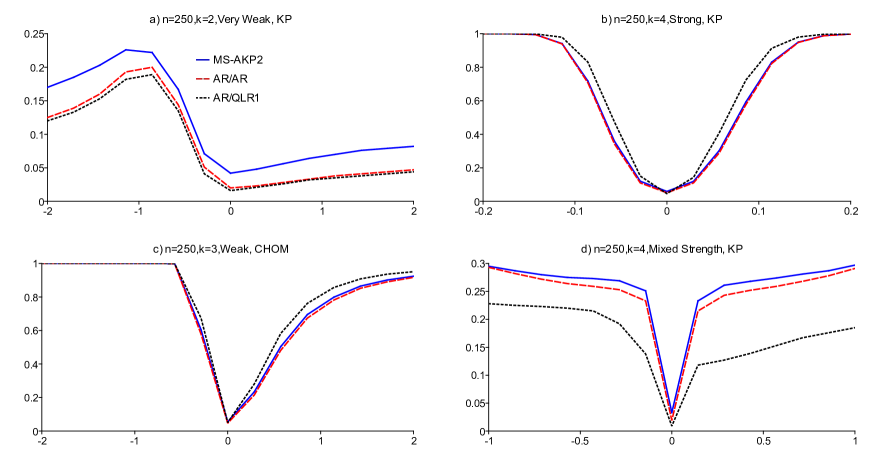
Figure 1: Power of various subvector tests in different cases. Covariance structure: Kronecker product (KP); CHOM. Identification strength $(\pi_{W},\pi_{Y})$: Very Weak $(2,2)$; Weak $(4,4)$; Strong $(40,40)$; Mixed strength: $(2,40)$.

A representative selection of power curves in four different cases is plotted in Figure 1. Note that in the figures corresponding to the different cases, both the scale of the horizontal and the vertical axes vary by a lot depending on the strength of identification.

The key takeaways from the power study are as follows:

i) Based on the DGPs considered here we cannot make a clear recommendation as to which one of the two tests MS-AKP1 and MS-AKP2 is preferable. In most cases, they have virtually identical power. In few cases, one dominates the other, but only by a small difference. In the Figures below we only report results for MS-AKP2.

ii) Regarding the comparison between the tests MS-AKP1, MS-AKP2 and AR/AR we find that the former two virtually uniformly dominate the latter in all the designs considered. This is not surprising given the construction of the new tests and given they satisfy Assumption RP above. The relative power advantage of the tests MS-AKP1, MS-AKP2 over AR/AR partly stems from the underrejection of the latter test under the null. See e.g. Figure 1a that contains power curves for $n=250,$ $k=2,$ very weak identification, and KP structure for MS-AKP2, AR/AR, and AR/QLR1. (The NRPs of the three tests reported here are 4.2, 2.0, and 1.6%, respectively. Note that the x-axis in Figures I-IV plots the true value $\beta.$)

iii) Regarding the comparison between the tests MS-AKP1, MS-AKP2 and AR/QLR1 in the case of equal identification strength $\pi_{W}=\pi_{Y}$ we find that the former two are generally more powerful under weak identification and small $k$ while the reverse is true under strong identification and larger $k,$ see Figures 1a and b for the cases “$k=2$ and very weak identification” and “$k=4$ and strong identification,” respectively, both for $n=250$ and KP. (In Figure 1b, the NRPs of the tests MS-AKP2, AR/AR, and AR/QLR1 are 5.9, 5.1, and 4.6%, respectively.) These two figures show the best relative performances for the MS-AKP1, MS-AKP2 and AR/QLR1 tests in the “equal identification” settings where $\pi_{W}=\pi_{Y}$. In Figure 1a the power advantage of MS-AKP2 over AR/QLR1 is as high as 5.2%, while in Figure 1b the power of AR/QLR1 can be up to 13.1% more powerful than MS-AKP2.

In the “intermediate” case between these extremes, namely “$k=3$ and weak identification” (again with $n=250$ and KP; not reported in Figure 1), the MS-AKP1 and MS-AKP2 tests have slightly higher power than AR/QLR1 when $\beta$ is positive while the reverse is true for negative values of $\beta$. In all cases, the relative performance of the AR/QLR1 test improves under CHOM; under CHOM, for the “intermediate” case “$k=3$ and weak identification” (again with $n=250$) the AR/QLR1 test has uniformly higher power than the MS-AKP1 and MS-AKP2 tests, see Figure 1c. (In Figure 1c, the NRPs of the tests MS-AKP2, AR/AR, and AR/QLR1 are 5.5, 4.7, and 5.1%, respectively.)

In cases of mixed identification strength, $\pi_{W}\neq\pi_{Y}\in\{2,40\},$ we find that when $\pi_{W}=2$ and $\pi_{Y}=40$ the tests MS-AKP1 and MS-AKP2 have uniformly higher power than AR/QLR1 for all $k$ considered whereas in the case $\pi_{W}=40$ and $\pi_{Y}=2$ all tests have comparable power. See Figure 1d that contains the case $\pi_{W}=2$ and $\pi_{Y}=40,$ $n=250,$ $k=4,$ with KP structure where the power gap between the new tests and AR/QLR1 is as high as 13.4%. (In Figure 1d, the NRPs of the tests MS-AKP2, AR/AR, and AR/QLR1 are 3.3, 1.9, and 0.9%, respectively.) It seems that in these cases of mixed identification strength the new tests enjoy their most competitive relative performance.

Results for non-KP DGPs

Finally, we examine how rejection probabilities are affected as the DGP transitions from KP to CHET outside of KP. To do so, we report rejection probabilities under the null and certain alternatives and probabilities with which MS-AKP1 and MS-AKP2 equals the AR/AR test in the second stage for a class of DGPs that under KP coincide with the ones considered in Figure 1b ($\pi_{W}=\pi_{Y}=40)$ and Figure 1d ($(\pi_{W},\pi_{Y})=(2,40))$. In particular, we choose $k=4,$ $n=250,$ $\gamma=0,$ and the matrix $\Sigma$ equals the one in (4.8). In (4.3) we take

$$Q_{\varepsilon}=I_{4}+\varrho\left(\begin{array}[c]{cccc}10&8&6&4\\ 3&5&9&3\\ 8&6&9&2\\ 4&3&2&1\end{array}\right)$$ (4.9)

for $\varrho\in\{0,.01,...,.1\},$ $\alpha_{\varepsilon}=\alpha_{V}=0,$ and $Q_{V}=I_{4}.$ Note that for $\varrho=0,$ the design leads to KP while for $\varrho>0,$ it leads to CHET outside of KP. In particular, $\arg\min_{G,H>0}||G\otimes H-\overline{R}_{F}||$ (with $\overline{R}_{F}$ defined in (2.4) with $U_{i}=(\varepsilon_{i},V_{W,i}^{\prime})^{\prime})$ equals $0,$ $.14,$ $.29,$ $.45,$ $.60,$ $.74,$ $.88,$ $1.01,$ $1.13,$ $1.24$, and $1.34$ when $\varrho\in\{0,.01,.02,....,.1\},$ respectively. The latter numbers are found by simulations based on $10^{7}$ simulation repetitions using Theorem 1 in GKM22.

As before, we report results for $10,000$ simulation repetitions at nominal size $5\%$.

Null rejection probabilities. Here we report results when $\beta=0,$ that is, we report NRPs.

First, in the setup of Figure 1b the probability with which MS-AKP1 and MS-AKP2 coincide with AR/AR is strictly increasing in $\varrho$ and e.g. equals 66.2% and 64.9%, 82.9% and 85.1%, and 98.8% and 99.5%, respectively for $\varrho=0,.03,$ and $.1$, respectively. (We also simulated these probabilities when $\varrho=0$ for $n=500$ and they equal 20.8% and 20.2%, respectively). The highest NRP of both the MS-AKP1 and MS-AKP2 tests is 5.9% which occurs when $\varrho=0$ and is caused by a 7.4% NRP of the conditional subvector test AR_AKP,α (even though by Theorem 1 this test has correct asymptotic NRP for this DGP; interestingly, this test has NRP equal to 5.8% when $\varrho=.1,$ a case that is not covered by Theorem 1). Given the MS-AKP1 and MS-AKP2 tests equal the AR/AR test with increasing probability as $\varrho$ increases, their NRPs get closer (but not monotonically so) to 5% as $\varrho$ increases. As $\varrho=.1$ both tests have NRP equal to 5.2%.

Second, in the setup of Figure 1d the probability with which MS-AKP1 and MS-AKP2 coincide with AR/AR are identical as just reported for the setup in Figure 1b. The highest NRPs of the MS-AKP1 and MS-AKP2 tests are 3.5% and 3.2% respectively, which occur when $\varrho=0$. The AR/AR and AR/QLR1 tests have NRPs in the intervals [1.2%,1.9%] and [.3%,.8%], respectively, and therefore, quite substantially underreject the null hypothesis. As the MS-AKP1 and MS-AKP2 tests equal the AR/AR test with increasing probability as $\varrho$ increases, their NRPs approach 1.2% as $\varrho$ gets closer to $.1.$

Power results. Here we examine how power is affected as the DGP transitions from KP to CHET outside of KP.

First, in the setup of Figure 1b) we consider the alternative $\beta=.1.$ The probabilities with which MS-AKP1 and MS-AKP2 coincide with AR/AR are increasing in $\varrho$ and are very similar to the corresponding values when $\beta=0;$ e.g. the probabilities equal 68.6% and 68.9% when $\varrho=.01$, respectively, and equal 98.2% and 99.1% when $\varrho=.1.$ Power for all tests monotonically decreases as $\varrho$ increases, e.g. for AR/QLR1, AR/AR, and MS-AKP1 from 83.5% to 44.4%, from 71.5% to 32.4% and from 72.5% to 32.4%, respectively, when $\varrho$ goes from 0 to .1.

Second, in the setup of Figure 1d) we consider the alternative $\beta=-1.$ When $\varrho=.01,$ MS-AKP1 and MS-AKP2 coincide with AR/AR with probability 78.3% and 75.5%, respectively and for $\varrho\geq.04$ both MS-AKP1 and MS-AKP2 coincide with AR/AR at least 99.6% of the cases. The power of the AR/AR and the AR/QLR1 for all values of $\varrho\in\{0,.01,.02,....,.1\}$ are in the intervals [27.9%,29.4%] and [21.2%,23.5%], respectively, with neither test’s power being monotonic in $\varrho.$ While the power of MS-AKP1 and MS-AKP2 slightly exceeds the power of the AR/AR test for $\varrho<.04$ their power is identical to the one of the AR/AR test for larger values of $\varrho.\vskip 3.0pt plus 1.0pt minus 1.0pt$

In sum, as one would expect given the construction of MS-AKP1 and MS-AKP2 tests, when moving from KP to CHET outside of KP, their rejection probabilities get closer and closer to those of the AR/AR test.

5 Conclusion

We propose the construction of a robust test that improves the power of another robust test by combining it with a powerful test that is only robust for a subset of the parameter space. We implement this construction in the context of the linear IV model applied to the AR_AKP,α test that has correct asymptotic size for a parameter space that imposes AKP structure and the AR/AR test that is robust even when allowing for arbitrary forms of CHET. We believe that the particular construction and implementation suggested here, namely combining a powerful but non fully robust test with a less powerful fully robust test in order to obtain a fully robust more powerful test, might be successfully applied in other scenarios and also in the current scenario based on different choices of testing procedures. For instance, it might be feasible to combine the LR type subvector test of Kleibergen (2021) with the AR/QLR1 of Andrews (2017) but it would be technically substantially more challenging to verify the assumptions given above that are sufficient for control of the asymptotic size of the resulting test. Other extensions include improving the power of the AR_AKP,α test by making the conditional critical value depend on more than just the largest eigenvalue.

Appendix A Appendix

The Appendix is structured as follows. In Section A.1 the proof of Theorem 1 is given, prepared for first with several technical lemmas in Subsection A.1.1. Next in Section A.2 the proof of Theorem 2 is given. We provide verifications of the high level assumptions for particular implementations of the test including for both $\varphi_{MS,c_{n}}$ and AR/AR in Sections A.3 and A.4, respectively. Finally, in Section A.5, we generalize the conditional subvector test to a time series framework.

A.1 Proof of Theorem 1

A.1.1 Technical lemmas

In what follows below we will require results about solutions to certain minimization problems involving the Frobenius norm. The next lemma provides a special case of Corollary 2.2 in van Loan and Pitsianis (1993). Note that van Loan and Pitsianis (1993) point to Golub and van Loan (1989, p.73) for a proof of Corollary 2.2. However, the result in Golub and van Loan (1989, p.73) is for a minimization problem using the $p$-norm for $p=2$ and not the Frobenius norm which is used here.

Lemma 2

Consider the minimization problem

$$\min_{B\in\Re^{m\times n},\text{ }rk(B)=1}||A-B||^{2}$$

for a given nonzero matrix $A\in\Re^{m\times n}$ with singular value decomposition $A=Udiag(\sigma_{1},...,\sigma_{p})V^{\prime}$ for singular values $\sigma_{1}\geq\sigma_{2}\geq...\geq\sigma_{p}\geq 0$ with $p=\min\{m,n\}$ and rectangular $diag(\sigma_{1},...,\sigma_{p})\in\Re^{m\times n}$, orthogonal matrices $U=[u_{1},...,u_{m}]\in\Re^{m\times m},$ and $V=[v_{1},...,v_{n}]\in\Re^{n\times n}.$ Then a minimizing argument is given by $B=\sigma_{1}u_{1}v_{1}^{\prime}$ and the minimum equals ${\textstyle\sum\nolimits_{i=2}^{p}}\sigma_{i}^{2}.$ If $\sigma_{1}>\sigma_{2}$ then $B=\sigma_{1}u_{1}v_{1}^{\prime}$ is the unique minimizer.

Proof of Lemma 2. Note that

$$\min_{B\in\Re^{m\times n},\text{ }rk(B)=1}||A-B||^{2}=\min_{C\in\Re^{m\times n},\text{ }rk(C)=1}||diag(\sigma_{1},...,\sigma_{p})-C||^{2}$$ (A.1)

by viewing $C=U^{\prime}BV$ and because $||D||=||U^{\prime}D||=||DV||$ for any matrix $D\in\Re^{m\times n}$ and conformable orthogonal matrices $U$ and $V.$ We can write any matrix $C\in\Re^{m\times n}$ with $rk(C)=1$ as

$$C=||c||^{-1}(\alpha_{1}c,...,\alpha_{n}c)$$ (A.2)

for $c\in\Re^{m}\backslash\{0^{m}\}$ and $\alpha_{k}\in\Re$ for $k=1,...,n.$ Because $||A+B||^{2}=||A||^{2}+||B||^{2}+2<A,B>_{F}$ where $<A,B>_{F}:=trace(A^{\prime}B)$ denotes the Frobenius inner product, and $||diag(\sigma_{1},...,\sigma_{p})||^{2}={\textstyle\sum\nolimits_{i=1}^{p}}\sigma_{i}^{2},$ $||C||^{2}={\textstyle\sum\nolimits_{i=1}^{n}}\alpha_{i}^{2},$ $<diag(\sigma_{1},...,\sigma_{p}),C>_{F}={\textstyle\sum\nolimits_{i=1}^{p}}\sigma_{i}\alpha_{i}c_{i}||c||^{-1}$ for $c=(c_{1},...,c_{m})^{\prime}$ we have

$$||diag(\sigma_{1},...,\sigma_{p})-C||^{2}={\textstyle\sum\nolimits_{i=1}^{p}}\sigma_{i}^{2}+{\textstyle\sum\nolimits_{i=1}^{n}}\alpha_{i}^{2}-2{\textstyle\sum\nolimits_{i=1}^{p}}\sigma_{i}\alpha_{i}c_{i}||c||^{-1}.$$ (A.3)

Viewing (A.3) as a function in $\alpha_{k},$ $k=1,...,n,$ and $c,$ taking first order conditions (FOCs) with respect to $\alpha_{k},$ we obtain $2\alpha_{k}-2\sigma_{k}c_{k}||c||^{-1}=0$ or

$$\alpha_{k}=\sigma_{k}c_{k}||c||^{-1}\text{ for }k=1,...,p\text{ and }\alpha_{k}=0\text{ for }k=p+1,...,n.$$ (A.4)

Taking FOCs with respect to $c_{j},$ $j=1,...,p,$ we obtain $(||c||\sigma_{j}\alpha_{j}-({\textstyle\sum\nolimits_{i=1}^{p}}\sigma_{i}\alpha_{i}c_{i})c_{j}||c||^{-1})||c||^{-2}=0$ and thus

$$||c||^{2}\sigma_{j}\alpha_{j}-({\textstyle\sum\nolimits_{i=1}^{p}}\sigma_{i}\alpha_{i}c_{i})c_{j}=0$$ (A.5)

and for $j=p+1,...,m$ we have $({\textstyle\sum\nolimits_{i=1}^{p}}\sigma_{i}\alpha_{i}c_{i})c_{j}||c||^{-3}=0$ and therefore

$$c_{j}{\textstyle\sum\nolimits_{i=1}^{p}}\sigma_{i}\alpha_{i}c_{i}=0.$$ (A.6)

The objective is to find $(c_{1},...,c_{p})$ such that the two summands in (A.3) that depend on $C$ are being minimized. Using (A.4) we thus need to find $(c_{1},...,c_{m})$ such that

$${\textstyle\sum\nolimits_{i=1}^{p}}\sigma_{i}^{2}c_{i}^{2}||c||^{-2}-2{\textstyle\sum\nolimits_{i=1}^{p}}\sigma_{i}^{2}c_{i}^{2}||c||^{-2}=-{\textstyle\sum\nolimits_{i=1}^{p}}\sigma_{i}^{2}(\frac{c_{i}}{||c||})^{2}$$ (A.7)

is minimized. Let $a$ be the largest index for which $\sigma_{1}=...=\sigma_{a}.$ Given that $\sigma_{a}>\sigma_{b}$ for $b>a$ it follows that a vector $c=(c_{1},...,c_{m})^{\prime}$ is a minimizing argument if and only if $(c_{1},...,c_{a})^{\prime}\neq 0^{m-p}$ and $(c_{a+1},...,c_{m})^{\prime}=0^{m-a}$ and the minimum in (A.3) equals

$${\textstyle\sum\nolimits_{i=1}^{p}}\sigma_{i}^{2}-{\textstyle\sum\nolimits_{i=1}^{p}}\sigma_{i}^{2}(\frac{c_{i}}{||c||})^{2}={\textstyle\sum\nolimits_{i=1}^{p}}\sigma_{i}^{2}-\sigma_{1}^{2}{\textstyle\sum\nolimits_{i=1}^{a}}(\frac{c_{i}}{||c||})^{2}={\textstyle\sum\nolimits_{i=2}^{p}}\sigma_{i}^{2}.$$ (A.8)

For example, one solution is $c=e_{1}:=(1,0,...0)^{\prime}\in\Re^{m}$ for which the minimizing matrix in (A.1) becomes $C=(\sigma_{1}e_{1},0^{m},...0^{m}).$ Correspondingly, a minimizing matrix $B$ becomes $UCV^{\prime}=\sigma_{1}u_{1}v_{1}^{\prime}.$

If $\sigma_{1}>\sigma_{2}$ then $a=1.$ Therefore, any minimizing $c$ equals $(c_{1},0,...,0)^{\prime}$ for some $c_{1}\neq 0$ and therefore, by (A.2) and (A.4), the only minimizing matrix $C$ equals $||c||^{-1}(\alpha_{1}c,...,\alpha_{n}c)=(\sigma_{1}e_{1},0^{m},...0^{m}).$ And consequently, there can only be a unique minimizer $B=UCV^{\prime}=\sigma_{1}u_{1}v_{1}^{\prime}.$ $\square$

Let $R\in\Re^{m\times l}$ and $R=U\Sigma V^{\prime}$ be a singular value decomposition of $R,$ where $\Sigma\in\Re^{m\times l}$ has $\min\{m,l\}$ singular values of $R$ on the diagonal and zeros elsewhere, $U\in\Re^{m\times m}$ is an orthogonal matrix of eigenvectors of $RR^{\prime},$ and $V\in\Re^{l\times l}$ is an orthogonal matrix of eigenvectors of $R^{\prime}R.$ In general, $U,$ $\Sigma,$ and $V$ are not uniquely defined. The matrix $\Sigma$ is uniquely determined by the restriction that the singular values are ordered nonincreasingly. We assume that this is the case from now on. Let $a$ be the geometric multiplicity of the largest eigenvalue of $RR^{\prime}.$ Write $U=[\widetilde{W}:\widetilde{W}^{C}]$ for $\widetilde{W}\in\Re^{m\times a}.$ Thus $\widetilde{W}=(\widetilde{w}_{1},...,\widetilde{w}_{a})$ denotes an orthogonal basis for the eigenspace associated with the largest eigenvalue of $RR^{\prime}$.

Lemma 3

Let $R$ and $R_{n}$ for $n\geq 1$ be $\Re^{m\times l}$ matrices such that $R_{n}\rightarrow R$ as $n\rightarrow\infty$. Let $U\Sigma V^{\prime}$ and $U_{n}\Sigma_{n}V_{n}^{\prime}$ be any singular value decompositions of $R$ and $R_{n},$ respectively, where the singular values are ordered nonincreasingly. For $j\leq m$, denote by $\widetilde{w}_{j}$ and $\widetilde{w}_{nj}$ the $j$-th column of $U$ and $U_{n},$ respectively. Decompose $U=[\widetilde{W}:\widetilde{W}^{C}]\in\Re^{m\times m},$ where $\widetilde{W}=(\widetilde{w}_{1},...,\widetilde{w}_{a})\in\Re^{m\times a}$ is an orthogonal basis for the eigenspace associated with the largest eigenvalue of $RR^{\prime}.$ Conformingly, let $U_{n}=[\widetilde{W}_{n}:\widetilde{W}_{n}^{C}].$ Assume $\Sigma$ does not equal the zero matrix. Then $\widetilde{w}_{nj}^{\prime}\widetilde{w}_{l}=o(1)$ for $j>a$ and $l\leq a$.

Proof of Lemma 3. Wlog we can assume $m\geq l.$ (If $m<l$ add $l-m$ rows of zeros to the bottom of $R$ and $R_{n}.$ Then the result for

$$\left(\begin{array}[c]{c}R\\ 0^{l-m\times l}\end{array}\right)=\left(\begin{array}[c]{cc}U&0^{m\times l-m}\\ 0^{l-m\times m}&\widetilde{U}\end{array}\right)\left(\begin{array}[c]{c}\Sigma\\ 0^{l-m\times l}\end{array}\right)V^{\prime}$$

for any orthogonal matrix $\widetilde{U}$ implies the desired result for $R=U\Sigma V^{\prime}.$) Denote by $\sigma_{j}$ the $j$-th singular value of $R$ (i.e. $\sigma_{j}$ equals the $(j,j)$-th element of $\Sigma$) for $j=1,...,l,$ and likewise $\sigma_{nj}$ denotes the $j$-th singular value of $R_{n}.$ By definition (and given that the algebraic and geometric multiplicities coincide for any diagonalizable matrix), $a$ is the largest index for which $\sigma_{1}=...=\sigma_{a}$. Define

$$\delta_{n}:=\min\{\min_{1\leq j\leq l-a}|\sigma_{a}-\sigma_{n(a+j)}|,\sigma_{a}\}.$$ (A.9)

Then by Wedin’s (1972) theorem (see, e.g. Li (1998) equations (4.4) and (4.8)), it follows that

$$||\sin\Theta(\widetilde{W},\widetilde{W}_{n})||=o(1/\delta_{n}),$$ (A.10)

where $\Theta(\widetilde{W},\widetilde{W}_{n})$ denotes the angle matrix between $\widetilde{W}$ and $\widetilde{W}_{n}$ (see Li (1998), equation (2.3) for a definition). Furthermore, by Lemma 2.1 and equation (2.4) in Li (1998), we have

$$||\sin\Theta(\widetilde{W},\widetilde{W}_{n})||=||\widetilde{W}_{n}^{C\prime}\widetilde{W}||.$$ (A.11)

Note that $\delta_{n}$ is bounded away from zero for all large $n$ because (1) $\sigma_{a}>0$ by the assumption that $\Sigma\neq 0,$ (2) if $a<l,$ by construction $\sigma_{a}>\sigma_{a+1}$ and therefore $\min_{1\leq j\leq l-a}|\sigma_{a}-\sigma_{n(a+j)}|$ is uniformly bounded away from zero (because singular values are continuous as functions of the matrix elements and $R_{n}\rightarrow R)$, and (3) if $a=l$ then $\min_{1\leq j\leq l-a}|\sigma_{a}-\sigma_{n(a+j)}|=\infty,$ because we take a minimum of the empty set. Therefore, by (A.10) and (A.11) we have

$$||\widetilde{W}_{n}^{C\prime}\widetilde{W}||=o(1)$$ (A.12)

which implies that $\widetilde{w}_{nj}^{\prime}\widetilde{w}_{l}=o(1)$ for $j>a$ and $l\leq a.$ $\square$

A.1.2 Uniformity Reparametrization

To prove that the new conditional subvector AR_AKP test has asymptotic size bounded by the nominal size $\alpha$ we use a general result in Andrews, Cheng, and Guggenberger (2020, ACG from now on). To describe it, consider a sequence of arbitrary tests $\{\varphi_{n}:n\geq 1\}$ of a certain null hypothesis and denote by $RP_{n}(\lambda)$ the NRP of $\varphi_{n}$ when the DGP is pinned down by the parameter vector $\lambda\in\Lambda,$ where $\Lambda$ denotes the parameter space of $\lambda.$ By definition, the asymptotic size of $\varphi_{n}$ is defined as

$$AsySz=\lim\sup_{n\rightarrow\infty}\sup_{\lambda\in\Lambda}RP_{n}(\lambda).$$ (A.13)

Let $\{h_{n}(\lambda):n\geq 1\}$ be a sequence of functions on $\Lambda,$ where $h_{n}(\lambda)=(h_{n,1}(\lambda),...,h_{n,J}(\lambda))^{\prime}$ with $h_{n,j}(\lambda)\in\Re$ $\forall j=1,...,J.$ Define

$$H\overset{}{=}\{h\overset{}{\in}(\Re\cup\{\pm\infty\})^{J}\overset{}{:}h_{w_{n}}(\lambda_{w_{n}})\overset{}{\rightarrow}h\text{ for some subsequence }\{w_{n}\}$$

$$\text{of }\{n\}\text{ and some sequence }\{\lambda_{w_{n}}\in\Lambda:n\geq 1\}\}.$$ (A.14)

Assumption B in ACG: For any subsequence $\{w_{n}\}$ of $\{n\}$ and any sequence $\{\lambda_{w_{n}}\in\Lambda:n\geq 1\}$ for which $h_{w_{n}}(\lambda_{w_{n}})\rightarrow h\in H,$ $RP_{w_{n}}(\lambda_{w_{n}})\rightarrow[RP^{-}(h),RP^{+}(h)]$ for some $RP^{-}(h),RP^{+}(h)\in(0,1).$

The assumption states, in particular, that along certain drifting sequences of parameters $\lambda_{w_{n}}$ indexed by a localization parameter $h$ the NRP of the test cannot asymptotically exceed a certain threshold $RP^{+}(h)$ indexed by $h.$

Proposition 4

$($ACG, Theorem 2.1$($a$)$ and Theorem 2.2$)$ Suppose Assumption B in ACG holds. Then, $\inf_{h\in H}RP^{-}(h)\leq AsySz\leq\sup_{h\in H}RP^{+}(h).$

We next verify Assumption B in ACG for the conditional subvector AR_AKP test and establish that $\sup_{h\in H}RP^{+}(h)=\alpha$ when the test is implemented at nominal size $\alpha$. In the setup considered here, the parameter space $\Lambda$ actually depends on $n$ which does not affect the conclusion of Theorem 2.1(a) and Theorem 2.2 in ACG.

We use Proposition 16.5 in AG, to derive the joint limiting distribution of the eigenvalues $\widehat{\kappa}_{in},$ $i=1,...,p$ in (2.25). We reparameterize the null distribution $F$ to a vector $\lambda.$ The vector $\lambda$ is chosen such that for a subvector of $\lambda$ convergence of a drifting subsequence of the subvector (after suitable renormalization) yields convergence of the NRP of the test. For given $F$ and any $G_{F}\in\Re^{p\times p}$ and $\overline{H}_{F}\in\Re^{k\times k}$ such that $\overline{R}_{F}=G_{F}\otimes\overline{H}_{F}+\Upsilon_{n}$ as in (2.5) define

$$U_{F}:=G_{F}^{-1/2}\in\Re^{p\times p}\text{ and }Q_{F}:=H_{F}^{-1/2}(E_{F}\overline{Z}_{i}\overline{Z}_{i}^{\prime})^{1/2}\in\Re^{k\times k},$$ (A.15)

where again $H_{F}=(E_{F}\overline{Z}_{i}\overline{Z}_{i}^{\prime})^{-1/2}\overline{H}_{F}(E_{F}\overline{Z}_{i}\overline{Z}_{i}^{\prime})^{-1/2}$ from (2.12). Denote by

$$B_{F}\in\Re^{p\times p}\text{ an orthogonal matrix of eigenvectors of }U_{F}^{\prime}(\Pi_{W}\gamma,\Pi_{W})^{\prime}Q_{F}^{\prime}Q_{F}(\Pi_{W}\gamma,\Pi_{W})U_{F}$$ (A.16)

ordered so that the $p$ corresponding eigenvalues $(\eta_{1F},...,\eta_{pF})$ are nonincreasing. Denote by

$$C_{F}\in\Re^{k\times k}\text{ an orthogonal matrix of eigenvectors of }Q_{F}(\Pi_{W}\gamma,\Pi_{W})U_{F}U_{F}^{\prime}(\Pi_{W}\gamma,\Pi_{W})^{\prime}Q_{F}^{\prime}.$$ (A.17)

The corresponding $k$ eigenvalues are $(\eta_{1F},...,\eta_{pF},0,...,0).$ Denote by

$$(\tau_{1F},...,\tau_{pF})\text{ the singular values of }Q_{F}(\Pi_{W}\gamma,\Pi_{W})U_{F}\in\Re^{k\times p},$$ (A.18)

which are nonnegative, ordered so that $\tau_{jF}$ is nonincreasing. (Some of these singular values may be zero.) As is well-known, the squares of the $p$ singular values of a $k\times p$ matrix $A$ equal the $p$ largest eigenvalues of $A^{\prime}A$ and $AA^{\prime}.$ In consequence, $\eta_{jF}=\tau_{jF}^{2}$ for $j=1,...,p.$ In addition, $\eta_{jF}=0$ for $j=p+1,...,k.$

Define the elements of $\lambda$ to be

$$\lambda_{1,F} :=(\tau_{1F},...,\tau_{pF})^{\prime}\in\Re^{p},$$

$$\lambda_{2,F} :=B_{F}\in\Re^{p\times p},$$

$$\lambda_{3,F} :=C_{F}\in\Re^{k\times k},$$

$$\lambda_{4,F} :=E_{F}\overline{Z}_{i}\overline{Z}_{i}^{\prime}\in\Re^{k\times k},$$

$$\lambda_{5,F} :=(\lambda_{5,1F},...,\lambda_{5,p-1F})^{\prime}:=\left(\frac{\tau_{2F}}{\tau_{1F}},...,\frac{\tau_{pF}}{\tau_{p-1F}}\right)^{\prime}\in[0,1]^{p-1},\text{ where }0/0:=0,$$

$$\lambda_{6,F} :=Q_{F}\in\Re^{k\times k},$$

$$\lambda_{7,F} :=U_{F}\in\Re^{p\times p},$$

$$\lambda_{8,F} :=F,\text{ and }$$

$$\lambda :=\lambda_{F}:=(\lambda_{1,F},...,\lambda_{8,F}).$$ (A.19)

Note that by (A.15) we have $G_{F}=U_{F}^{-2}=\lambda_{7,F}^{-2}$ and $H_{F}=(E_{F}\overline{Z}_{i}\overline{Z}_{i}^{\prime})^{1/2}Q_{F}^{-1}Q_{F}^{\prime-1}(E_{F}\overline{Z}_{i}\overline{Z}_{i}^{\prime})^{1/2}$ $=\lambda_{4,F}^{1/2}\lambda_{6,F}^{-1}\lambda_{6,F}^{{}^{\prime}-1}\lambda_{4,F}^{1/2}.$ In Section 3 the additional element $\lambda_{9,F}$ defined in (3.2) is appended to $\lambda$ with corresponding changes to several objects below, e.g. $\Lambda_{n}$ and $h_{n}(\lambda)$ in (A.20) and $\lambda_{w_{n},h}$ in (A.19) and (A.21); e.g. $h_{n}(\lambda)$ becomes $(n^{1/2}\lambda_{1,F},\lambda_{2,F},\lambda_{3,F},...,\lambda_{7,F},\lambda_{9,F}).$

The parameter space $\Lambda_{n}$ for $\lambda$ and the function $h_{n}(\lambda)$ (that appears in Assumption B in ACG) are defined by

$$\Lambda_{n} :=\{\lambda:\lambda=(\lambda_{1,F},...,\lambda_{8,F})\text{ for some }F\text{ st }(\gamma,\Pi_{W},\Pi_{Y},F)\in\mathcal{F}_{AKP,a_{n}}\text{ for some }(\gamma,\Pi_{W},\Pi_{Y})\},$$

$$h_{n}(\lambda) :=(n^{1/2}\lambda_{1,F},\lambda_{2,F},\lambda_{3,F},...,\lambda_{7,F}).$$ (A.20)

We define $\lambda$ and $h_{n}(\lambda)$ as in (A.19) and (A.20) because, as shown below, the asymptotic distributions of the test statistic and conditional critical values under a sequence $\{F_{n}:n\geq 1\}$ for which $h_{n}(\lambda_{F_{n}})\rightarrow h$ depend on $\lim n^{1/2}\lambda_{1,F_{n}}$ and $\lim\lambda_{m,F_{n}}$ for $m=2,...,7.$ Note that we can view $h\in\left(\Re\cup\{\pm\infty\}\right)^{J}$ (for an appropriately chosen finite $J\in N$).

For notational convenience, for any subsequence $\{w_{n}:n\geq 1\},$

$$\{\lambda_{w_{n},h}:n\geq 1\}\text{ denotes a sequence }\{\lambda_{w_{n}}\in\Lambda_{n}:n\geq 1\}\text{ for which }h_{w_{n}}(\lambda_{w_{n}})\rightarrow h.$$ (A.21)

It follows that the set $H$ defined in (A.14) is given as the set of all $h\in(\Re\cup\{\pm\infty\})^{J}$ such that there exists $\{\lambda_{w_{n},h}:n\geq 1\}$ for some subsequence $\{w_{n}:n\geq 1\}.$

We decompose $h$ analogously to the decomposition of the first seven components of $\lambda$: $h=(h_{1},...,h_{7}),$ where $\lambda_{m,F}$ and $h_{m}$ have the same dimensions for $m=1,...,7.$ We further decompose the vector $h_{1}$ as $h_{1}=(h_{1,1},...,h_{1,p})^{\prime},$ where the elements of $h_{1}$ could equal $\infty.$ Again, by definition, under a sequence $\{\lambda_{n,h}:n\geq 1\},$ we have

$$n^{1/2}\tau_{jF_{n}}\rightarrow h_{1,j}\geq 0\text{ }\forall j=1,...,p,\text{ }\lambda_{m,F_{n}}\rightarrow h_{m}\text{ }\forall m=2,...,7.$$ (A.22)

Note that $h_{1,p}=\tau_{pF_{n}}=0$ because $\rho(\Pi_{W}\gamma,\Pi_{W})<p,$ where $\rho(A)$ denotes the rank of a matrix $A.$

By Lyapunov-type WLLNs and CLTs, using the moment restrictions imposed in (2.5), we have under $\lambda_{n,h}$

$$\left(\begin{array}[c]{c}n^{-1/2}\overline{Z}^{\prime}(\varepsilon+V_{W}\gamma_{n})\\ vec\left(n^{-1/2}\overline{Z}^{\prime}V_{W}\right)\end{array}\right)\overset{}{\underset{d}{\rightarrow}}\left(\begin{array}[c]{c}\xi_{1,h}\\ \xi_{2,h}\end{array}\right)\overset{}{\sim}N\left(0^{kp},\left(h_{7}^{-2}\otimes(h_{4}h_{6}^{-1}h_{6}^{\prime-1}h_{4})\right)\right),$$ (A.27)

$$\lambda_{4,F_{n}}^{-1}(n^{-1}\overline{Z}^{\prime}\overline{Z})\overset{}{\underset{p}{\rightarrow}}I_{k},\text{ }n^{-1}\overline{Z}^{\prime}[\varepsilon\overset{}{:}V_{W}]\overset{}{\underset{p}{\rightarrow}}0^{k\times p},$$ (A.28)

where the random vector $(\xi_{1,h},\xi_{2,h}^{\prime})^{\prime}$ is defined here, $F_{n}$ denotes the distribution of $(\varepsilon_{i},\overline{Z}_{i}^{\prime},V_{Y,i}^{\prime}V_{W,i}^{\prime})$ under $\lambda_{n,h},$ and, by definition above, $h_{7}^{-2}$ and $h_{4}h_{6}^{-1}h_{6}^{\prime-1}h_{4}$ denote the limits of $G_{F_{n}}$ and $\overline{H}_{F_{n}}$ under $\lambda_{n,h}.$

Let $q=q_{h}\in\{0,...,p-1\}$ be such that

$$h_{1,j}=\infty\text{ for }1\leq j\leq q_{h}\text{ and }h_{1,j}<\infty\text{ for }q_{h}+1\leq j\leq p,$$ (A.29)

where $h_{1,j}:=\lim n^{1/2}\tau_{jF_{n}}\geq 0$ for $j=1,...,p$ by (A.22) and the distributions $\{F_{n}:n\geq 1\}$ correspond to $\{\lambda_{n,h}:n\geq 1\}$ defined in (A.21). This value $q$ exists because $\{h_{1,j}:j\leq p\}$ are nonincreasing in $j$ (since $\{\tau_{jF}:j\leq p\}$ are nonincreasing in $j,$ as defined in (A.18)). Note that $q$ is the number of singular values of $Q_{F_{n}}(\Pi_{Wn}\gamma_{n},\Pi_{Wn})U_{F_{n}}\in\Re^{k\times p}$ that diverge to infinity when multiplied by $n^{1/2}.$ Note again that $q<p$ because $\rho(\Pi_{Wn}\gamma_{n},\Pi_{Wn})<p.$

A.1.3 Asymptotic Distributions

One might wonder whether the definition of $\widehat{G}_{n}$ in $($2.23$)$ as $vec(\widehat{G}_{n})=\widehat{L}(:,1)/\widehat{L}(1,1)$ where $(\widehat{G}_{n},\widehat{H}_{n})$ are minimizers in (2.13) is unique. If for instance the eigenspace corresponding to the largest eigenvalue was of dimension bigger than one, then clearly $\widehat{L}(:,1)$ would not be uniquely defined. The following lemma shows that the definition of $\widehat{G}_{n}$ is unique and derives its limit.

To simplify notation a bit, we write shorthand $R_{n}$ for $R_{F_{n}}$ and likewise for other expressions.

Lemma 4

Under sequences $\lambda_{n,h}$ from $\Lambda_{n}$ in $($A.20$)$ based on the parameter space $\mathcal{F}_{AKP,a_{n}}$, wp1 the definition of $\widehat{G}_{n}\in\Re^{p\times p}$ and $\widehat{H}_{n}\in\Re^{k\times k}$ in $($2.23$)$ is unique and

$$\widehat{G}_{n}\rightarrow\lim_{n\rightarrow\infty}G_{n}\text{ and }\widehat{H}_{n}\rightarrow\lim_{n\rightarrow\infty}H_{n}\text{ a.s.,}$$

where $H_{n}=(E_{F_{n}}\overline{Z}_{i}\overline{Z}_{i}^{\prime})^{-1/2}\overline{H}_{n}(E_{F_{n}}\overline{Z}_{i}\overline{Z}_{i}^{\prime})^{-1/2}$ is defined in $($2.12$).$

Comment. Note that under sequences $\lambda_{n,h},$ $\lim_{n\rightarrow\infty}G_{n}$ and $\lim_{n\rightarrow\infty}H_{n}$ do exist. On the other hand, the matrices $G_{n}$ and $H_{n}$ may not be uniquely pinned down by the restrictions in (2.5) in $\mathcal{F}_{AKP,a_{n}}$. The results $\widehat{G}_{n}\rightarrow\lim_{n\rightarrow\infty}G_{n}$ and $\widehat{H}_{n}\rightarrow\lim_{n\rightarrow\infty}H_{n}$ a.s. hold for any possible choice of $G_{n}$ and $H_{n}.\vskip 6.0pt plus 2.0pt minus 2.0pt$

Proof of Lemma 4. Recall the definition

$$R_{n}=(I_{p}\otimes(E_{F_{n}}\overline{Z}_{i}\overline{Z}_{i}^{\prime})^{-1/2})E_{F_{n}}(vec(\overline{Z}_{i}U_{i}^{\prime})(vec(\overline{Z}_{i}U_{i}^{\prime}))^{\prime})(I_{p}\otimes(E_{F_{n}}\overline{Z}_{i}\overline{Z}_{i}^{\prime})^{-1/2})$$ (A.30)

in (2.10). By Theorem 1 in van Loan and Pitsianis (1993),

$$||A-B\otimes C||=||\mathcal{R}(A)-vec(B)vec(C)^{\prime}||$$ (A.31)

for any conformable matrices $A,B,$ and $C.$ Thus, for

$$\overline{\Upsilon}_{n}:=(I_{p}\otimes(E_{F_{n}}\overline{Z}_{i}\overline{Z}_{i}^{\prime})^{-1/2})\Upsilon_{n}(I_{p}\otimes(E_{F_{n}}\overline{Z}_{i}\overline{Z}_{i}^{\prime})^{-1/2}),$$ (A.32)

it follows that $\mathcal{R}(R_{n}-\overline{\Upsilon}_{n})=vec(G_{n})vec(H_{n})^{\prime}$ and because $\kappa_{\min}(E_{F_{n}}\overline{Z}_{i}\overline{Z}_{i}^{\prime})^{-1/2}),$ $\kappa_{\min}(G_{n}),$ and $\kappa_{\min}(\overline{H}_{n})\geq\delta_{2}$ in $\mathcal{F}_{AKP,a_{n}},$ it follows that $\mathcal{R}(R_{n}-\overline{\Upsilon}_{n})$ has rank 1. It follows also that $\lim_{n\rightarrow\infty}\mathcal{R}(R_{n}-\overline{\Upsilon}_{n})=\lim_{n\rightarrow\infty}\mathcal{R}(R_{n})$ (which exists under sequences $\lambda_{n,h}$) has rank 1 (even though the rank of $\mathcal{R}(R_{n})$ could be larger than 1 for every $n$). By continuity of the singular values and because the geometric and algebraic multiplicity coincide for diagonalizable matrices, the dimension of the eigenspace of $\mathcal{R}(R_{n})\mathcal{R}(R_{n})^{\prime}$ corresponding to the largest singular value of $\mathcal{R}(R_{n})$ is one for all $n$ large enough.

By the uniform moment restrictions in (2.5) in $\mathcal{F}_{AKP,a_{n}},$ namely $E_{F}(||T_{i}||^{2+\delta_{1}})\leq B<\infty,$ for $T_{i}\in\{vec(\overline{Z}_{i}U_{i}^{\prime}),vec(\overline{Z}_{i}\overline{Z}_{i}^{\prime})\}$ and $\kappa_{\min}(E_{F}(\overline{Z}_{i}\overline{Z}_{i}^{\prime}))\geq\delta_{2}>0,$ a strong law of large numbers implies that

$$\widehat{R}_{n}-R_{n}\rightarrow 0^{kp\times kp}\text{ and }\mathcal{R}(\widehat{R}_{n})-\mathcal{R}(R_{n})\rightarrow 0^{pp\times kk}\text{ a.s.}$$ (A.33)

Therefore, the dimension of the eigenspace of $\mathcal{R}(\widehat{R}_{n})\mathcal{R}(\widehat{R}_{n})^{\prime}$ corresponding to the largest singular value of $\mathcal{R}(\widehat{R}_{n})$ is one for all $n$ large enough wp1.

By the uniqueness statement of Lemma 2 for the rank 1 case, it follows that the formula for minimizers of the KP approximation problem in (2.13) given in van Loan and Pitsianis (1993, Corollary 2 and Theorem 11), namely

$$vec(\widehat{G}_{n})=\widehat{\sigma}_{1}\widehat{L}(:,1)\text{ and }vec(\widehat{H}_{n})=\widehat{N}(:,1),$$ (A.34)

yields symmetric pd matrices $\widehat{G}_{n}$ and $\widehat{H}_{n}.$ When applying Theorem 11, note that $\widehat{R}_{n}>0$ for all large enough $n$ wp1, which holds by (A.33), $\lim_{n\rightarrow\infty}G_{n}\otimes H_{n}=\lim_{n\rightarrow\infty}R_{n}-\overline{\Upsilon}_{n}=\lim_{n\rightarrow\infty}R_{n},$ and because $\kappa_{\min}(E_{F_{n}}\overline{Z}_{i}\overline{Z}_{i}^{\prime})^{-1/2}),$ $\kappa_{\min}(G_{n}),$ and $\kappa_{\min}(\overline{H}_{n})\geq\delta_{2}$ in $\mathcal{F}_{AKP,a_{n}}$. Given that $\widehat{G}_{n}>0,$ Sylvester’s criterion for positive definiteness implies that $\widehat{L}(1,1)>0$ for all large enough $n$ wp1, and we can therefore define $\widehat{G}_{n}$ and $\widehat{H}_{n}$ as in $($2.23$)$ with normalization to 1 of the upper left element of $\widehat{G}_{n}$ for all large enough $n$ wp1.

Next we apply Lemma 3 with $a=1$ and the roles of $R_{n}$ and $R$ in Lemma 3 played by $\mathcal{R}(\widehat{R}_{n})$ and $\lim_{n\rightarrow\infty}\mathcal{R}(R_{n})$, respectively. By (A.33), the lemma implies

$$\widehat{L}(:,j)^{\prime}L_{1}=o(1)$$ (A.35)

wp1. for $j>1$, where $\widehat{L}(:,j)$ denotes the $j$-th column of $\widehat{L}$ in the singular value decomposition $\widehat{L}^{\prime}\mathcal{R}(\widehat{R}_{n})\widehat{N}=diag(\widehat{\sigma}_{l})$ of $\mathcal{R}(\widehat{R}_{n})$ and $L_{1}$ denotes the first column of $\overline{L}$ in the singular value decomposition $\overline{L}^{\prime}\mathcal{R}(\lim_{n\rightarrow\infty}\mathcal{R}(R_{n}))\overline{N}=diag(\overline{\sigma}_{l})$ of $\lim_{n\rightarrow\infty}\mathcal{R}(R_{n}).$ For any orthogonal basis $(x_{1},...,x_{p^{2}})$ of $\Re^{p^{2}}$ and $y\in\Re^{p^{2}}$ we have $y={\textstyle\sum\nolimits_{j=1}^{p^{2}}}(y^{\prime}x_{j})x_{j}.$ In particular, we have $L_{1}={\textstyle\sum\nolimits_{j=1}^{p^{2}}}(L_{1}^{\prime}\widehat{L}(:,j))\widehat{L}(:,j)=(L_{1}^{\prime}\widehat{L}(:,1))\widehat{L}(:,1)+o(1)$ wp1., where the second equality holds by (A.35). Together with the normalization of the upper left elements of $\widehat{G}_{n}$ and $G_{n}$ to 1, this implies $\widehat{G}_{n}-G_{n}\rightarrow 0^{p\times p}$ a.s. and $\widehat{H}_{n}-H_{n}\rightarrow 0^{k\times k}$ a.s. follows analogously. $\square$

An analogue to Lemma 16.4 in AG and Lemma 1 in GKM19 is given by the following statement. Define

$$\widehat{D}_{n}:=(\overline{Z}^{\prime}\overline{Z})^{-1}\overline{Z}^{\prime}\left(\overline{Y}_{0},W\right)\text{ and }\widehat{Q}_{n}:=\widehat{H}_{n}^{-1/2}(n^{-1}\overline{Z}^{\prime}\overline{Z})^{1/2}\text{.}$$ (A.36)

Denote by $vec_{k,m_{W}}^{-1}(\cdot)$ the inverse $vec$ operation that transforms a $km_{W}$ vector into a $k\times m_{W}$ matrix.

Lemma 5

Under sequences $\{\lambda_{n,h}:n\geq 1\}$ with $\lambda_{n,h}\in\Lambda_{n}$ in $($A.20$)$ based on the parameter space $\mathcal{F}_{AKP,a_{n}},$ $n^{1/2}(\widehat{D}_{n}-(\Pi_{Wn}\gamma_{n},\Pi_{Wn}))\rightarrow_{d}\overline{D}_{h},$ where

$$\overline{D}_{h}\sim h_{4}^{-1}(\xi_{1,h},vec_{k,m_{W}}^{-1}(\xi_{2,h})),$$

$\xi_{1,h}$ and $\xi_{2,h}$ are defined in $($A.28$)$, and again $h_{4}$ is the limit of $\lambda_{4,n}=E_{F_{n}}\overline{Z}_{i}\overline{Z}_{i}^{\prime}.$ Furthermore, we have $\widehat{Q}_{n}-Q_{n}\rightarrow_{p}0^{k\times k}$.

Proof of Lemma 5. We have

$$n^{1/2}(\widehat{D}_{n}-(\Pi_{Wn}\gamma_{n},\Pi_{Wn}))$$

$$=n^{1/2}((\overline{Z}^{\prime}\overline{Z})^{-1}\overline{Z}^{\prime}(y-Y\beta_{0},W)-(\Pi_{Wn}\gamma_{n},\Pi_{Wn}))$$

$$=n^{1/2}((\overline{Z}^{\prime}\overline{Z})^{-1}\overline{Z}^{\prime}(\overline{Z}\Pi_{Wn}\gamma_{n}+V_{W}\gamma_{n}+\varepsilon,\overline{Z}\Pi_{Wn}+V_{W})-(\Pi_{Wn}\gamma_{n},\Pi_{Wn}))$$

$$=(n^{-1}\overline{Z}^{\prime}\overline{Z})^{-1}[n^{-1/2}\overline{Z}^{\prime}(V_{W}\gamma_{n}+\varepsilon,V_{W})]\rightarrow_{d}\overline{D}_{h},$$ (A.37)

where the first equality uses the definition of $\widehat{D}_{n}$ in (A.36), the second equality uses the formulas in (2.1), and the convergence results holds by the (triangular array) CLT and WLLN in (A.28). The remaining statement holds by the WLLN in (A.28) and the consistency of $\widehat{H}_{n}$ for $H_{n}$ proven above. $\square\vskip 6.0pt plus 2.0pt minus 2.0pt$

For notational convenience, write

$$\widehat{U}_{n}:=\widehat{G}_{n}^{-1/2}.$$ (A.38)

Note that the matrix $n\widehat{U}_{n}\widehat{D}_{n}^{\prime}\widehat{Q}_{n}^{\prime}\widehat{Q}_{n}\widehat{D}_{n}\widehat{U}_{n}$ equals $n^{-1}\widehat{G}_{n}^{-1/2}\left(\overline{Y}_{0},W\right)^{\prime}Z\widehat{H}_{n}^{-1}Z^{\prime}\left(\overline{Y}_{0},W\right)\widehat{G}_{n}^{-1/2}$ which appears in (2.25). Thus, $\widehat{\kappa}_{in}$ for $i=1,...,p$ equals the $i$th eigenvalue of $n\widehat{U}_{n}^{\prime}\widehat{D}_{n}^{\prime}\widehat{Q}_{n}^{\prime}\widehat{Q}_{n}\widehat{D}_{n}\widehat{U}_{n},$ ordered nonincreasingly, and $\widehat{\kappa}_{pn}$ is the subvector AR_AKP test statistic. To describe the limiting distribution of $(\widehat{\kappa}_{1n},...,\widehat{\kappa}_{pn})$ we need additional notation, namely:

$$h_{2} =(h_{2,q},h_{2,p-q}),\text{ }h_{3}=(h_{3,q},h_{3,k-q}),$$

$$h_{1,p-q}^{\diamond}\overset{}{:} =\left[\begin{array}[c]{c}0^{q\times(p-q)}\\ Diag\{h_{1,q+1},...,h_{1,p-1},0\}\\ 0^{(k-p)\times(p-q)}\end{array}\right]\in\Re^{k\times(p-q)},$$ (A.42)

$$\overline{\Delta}_{h}\overset{}{:} =(\overline{\Delta}_{h,q},\overline{\Delta}_{h,p-q})\in\Re^{k\times p},\text{ }\overline{\Delta}_{h,q}:=h_{3,q}\in\Re^{k\times q},\text{ }$$

$$\overline{\Delta}_{h,p-q} :=h_{3}h_{1,p-q}^{\diamond}+h_{6}\overline{D}_{h}h_{7}h_{2,p-q}\in\Re^{k\times(p-q)},$$ (A.43)

where $h_{2,q}\in\Re^{p\times q},$ $h_{2,p-q}\in\Re^{p\times(p-q)},$ $h_{3,q}\in\Re^{k\times q},$ $h_{3,k-q}\in\Re^{k\times(k-q)},$ $\overline{\Delta}_{h,q}\in\Re^{k\times q},$ and $\overline{\Delta}_{h,p-q}\in\Re^{k\times(p-q)}$. Let $T_{n}:=B_{F_{n}}S_{n}$ and $S_{n}:=Diag\{(n^{1/2}\tau_{1F_{n}})^{-1},...,(n^{1/2}\tau_{qF_{n}})^{-1},1,...,1\}\in\Re^{p\times p}.$ The same proof as the one of Lemma 16.4 in AG shows that $n^{1/2}Q_{F_{n}}\widehat{D}_{n}U_{F_{n}}T_{n}\rightarrow_{d}\overline{\Delta}_{h}$ under all sequences $\{\lambda_{n,h}:n\geq 1\}$ with $\lambda_{n,h}\in\Lambda$. The following proposition is an analogue to Proposition 16.5 in AG and to Proposition 2 in GKM19.

Proposition 5

Under all sequences $\{\lambda_{n,h}:n\geq 1\}$ with $\lambda_{n,h}\in\Lambda_{n},$

$($a$)$ $\widehat{\kappa}_{jn}\rightarrow_{p}\infty$ for all $j\leq q,$

$($b$)$ the $($ordered$)$ vector of the smallest $p-q$ eigenvalues of $n\widehat{U}_{n}^{\prime}\widehat{D}_{n}^{\prime}\widehat{Q}_{n}\widehat{Q}_{n}\widehat{D}_{n}\widehat{U}_{n},$ i.e., $(\widehat{\kappa}_{(q+1)n},...,\allowbreak\widehat{\kappa}_{pn})^{\prime},$ converges in distribution to the $($ordered$)$ $p-q\$vector of the eigenvalues of $\overline{\Delta}_{h,p-q}^{\prime}h_{3,k-q}h_{3,k-q}^{\prime}\overline{\Delta}_{h,p-q}\in\Re^{(p-q)\times(p-q)},$

$($c$)$ the convergence in parts (a) and (b) holds jointly with the convergence in Lemma 5, and

$($d$)$ under all subsequences $\{w_{n}\}$ and all sequences $\{\lambda_{w_{n},h}:n\geq 1\}$ with $\lambda_{w_{n},h}\in\Lambda_{n},$ the results in parts $($a$)$-$($c$)$ hold with $n$ replaced with $w_{n}.$

Comments. 1. The proof of the proposition follows from the proof of Proposition 16.5 in AG. Note that Assumption WU in AG (assumed in their Proposition 16.5) is fulfilled with the roles of $W_{2F},$ $W_{F},$ $U_{2F},$ and $U_{F}$ in AG played here by $Q_{F},$ $Q_{F},$ $U_{F},$ and $U_{F},$ respectively, while the roles of $W_{1}$ and $U_{1}$ in AG are played by the identity function. The roles of $\widehat{W}_{2n}$ and $\widehat{W}_{n}$ in AG are both played by $\widehat{Q}_{n}$ and those of both $\widehat{U}_{2n}$ and $\widehat{U}_{n}$ by $\widehat{U}_{n}$. Lemma 5 then shows consistency $\widehat{W}_{2n}-W_{2F_{n}}\rightarrow_{p}0^{k\times k}$ and $\widehat{U}_{2n}-U_{2F_{n}}\rightarrow_{p}0^{p\times p}$ under sequences $\{\lambda_{n,h}:n\geq 1\}$ with $\lambda_{n,h}\in\Lambda_{n}$ and trivially the functions $W_{1}$ and $U_{1}$ are continuous in our case. Note that by the restrictions in $\mathcal{F}_{AKP,a_{n}}$ in (2.5) the requirements in the parameter space $F_{WU}$ in AG, namely “$\kappa_{\min}(Q_{F})$ and $\kappa_{\min}(U_{F})$ are uniformly bounded away from zero and $||Q_{F}||$ and $||U_{F}||$ are uniformly bounded away from infinity”, are fulfilled. For example, the former follows because $\kappa_{\min}(Q_{F})=1/\kappa_{\max}(Q_{F}^{-1})=1/\kappa_{\max}((E_{F}\overline{Z}_{i}\overline{Z}_{i}^{\prime})^{-1/2}H_{F}^{1/2})$ and $\kappa_{\max}((E_{F}\overline{Z}_{i}\overline{Z}_{i}^{\prime})^{-1/2}H_{F}^{1/2})$ is uniformly bounded.

2. Proposition 5 yields the desired joint limiting distribution of the $p$ eigenvalues in (2.25). Using repeatedly the general formula $(C^{\prime}\otimes A)vec(B)=vec(ABC)$ for three conformable matrices $A,B,C,$ we have for the expression $h_{6}\overline{D}_{h}h_{7}$ that appears in $\overline{\Delta}_{h,p-q}$

$$vec(h_{6}\overline{D}_{h}h_{7})=vec(h_{6}h_{4}^{-1}(\xi_{1,h},vec_{k,m_{W}}^{-1}(\xi_{2,h}))h_{7})=(h_{7}\otimes(h_{4}h_{6}^{-1})^{-1})\left(\begin{array}[c]{c}\xi_{1,h}\\ \xi_{2,h}\end{array}\right)$$ (A.46)

$$\sim vec(v_{1},...,v_{p}),$$ (A.47)

where, by definition, $v_{j},$ $j=1,...,p$ are i.i.d. normal $k$-vectors with zero mean and covariance matrix $I_{k},$ and the distributional statement follows by straightforward calculations using (A.28). Therefore, by Lemma 5, the definition of $\overline{\Delta}_{h,p-q}$ in (A.43), and by noting that

$$h_{3,k-q}^{\prime}h_{3}h_{1,p-q}^{\diamond}=\left(\begin{array}[c]{c}Diag\{h_{1,q+1},...,h_{1,p-1},0\}\\ 0^{(k-p)\times(p-q)}\end{array}\right)$$ (A.48)

we obtain

$$h_{3,k-q}^{\prime}\overline{\Delta}_{h,p-q} =\left(\begin{array}[c]{c}Diag\{h_{1,q+1},...,h_{1,p-1},0\}\\ 0^{(k-p)\times(p-q)}\end{array}\right)+h_{3,k-q}^{\prime}(v_{1},...,v_{p})h_{2,p-q}$$ (A.51)

$$\sim\left(\begin{array}[c]{c}Diag\{h_{1,q+1},...,h_{1,p-1},0\}\\ 0^{(k-p)\times(p-q)}\end{array}\right)+(w_{1},...,w_{p-q}),$$ (A.54)

where, by definition, $w_{j},$ $j=1,...,p-q$ are i.i.d. normal $(k-q)$-vectors with zero mean and covariance matrix $I_{k-q}.$ The distributional equivalence in the second line holds because $(v_{1},...,v_{p})h_{2,p-q}\sim(\widetilde{v}_{1},...,\widetilde{v}_{p-q}),$ where $\widetilde{v}_{j},$ $j=1,...,p-q$ are i.i.d. $N(0^{k},I_{k})$ as $h_{2,p-q}$ has orthogonal columns of length 1. Analogously, $h_{3,k-q}^{\prime}(\widetilde{v}_{1},...,\widetilde{v}_{p-q})\sim(w_{1},...,w_{p-q})$ because $h_{3,k-q}$ has orthogonal columns of length 1.

For example, when $q=p-1=m_{W}$ (which could be called the ”strong IV” case), we obtain from (A.54) $h_{3,k-q}^{\prime}\overline{\Delta}_{h,p-q}=w_{1}\in\Re^{k-m_{W}}.$ Therefore $\overline{\Delta}_{h,p-q}^{\prime}h_{3,k-q}h_{3,k-q}^{\prime}\overline{\Delta}_{h,p-q}\sim\chi_{k-m_{W}}^{2}$ and thus by part (b) of Proposition 5 the limiting distribution of the subvector AR_AKP test statistic is $\chi_{k-m_{W}}^{2}$ in that case, while all the larger roots in (2.25) converge in probability to infinity by part (a).

Proof of Theorem 1. Given the discussion in Comment 2 to Proposition 5, the same proof as for Theorem 5 in GKM19 applies. $\square$

A.2 Proof of Theorem 2

Proof of Theorem 2. It is enough to verify Proposition 4 above for the parameter space $\mathcal{F}_{Het}$ and the test $\varphi_{MS-AKP,\alpha}.$ To verify Assumption B in ACG consider a sequence $\lambda_{w_{n},h}$ defined as in (A.19) and (A.21) above except that the component

$$\lambda_{9w_{n}}:=\min||R_{F_{w_{n}}}^{-1/2}(G\otimes H-R_{F_{w_{n}}})R_{F_{w_{n}}}^{-1/2}||/c_{w_{n}}$$ (A.55)

is added to $\lambda_{w_{n}}$, where the minimum (here and in similar expressions below) is taken over $(G,H)$ for $G\in\Re^{p\times p},$ $H\in\Re^{k\times k}$ being pd, symmetric matrices, normalized such that the upper left element of $G$ equals 1. In (A.20), we replace $\mathcal{F}_{AKP,a_{w_{n}}}$ by $\mathcal{F}_{Het}$ and define $h_{w_{n}}(\lambda_{F}):=(w_{n}^{1/2}\lambda_{1,F},\lambda_{2,F},\lambda_{3,F},\ldots,\allowbreak\lambda_{7,F},w_{n}^{1/2}\lambda_{9,F}).$ To simplify notation, we write $n$ instead of $w_{n}$ from now on.

Consider first a sequence $\lambda_{n,h}$ with $h_{9}=\infty.$ By Assumption MS, $\varphi_{MS,c_{n}}=1$ wpa1 and therefore, $\varphi_{MS-AKP,\alpha}=\varphi_{Rob,\alpha-\delta}$ wpa1. Thus, the new test $\varphi_{MS-AKP,\alpha}$ has limiting NRP bounded by $\alpha-\delta$ in that case because $\varphi_{Rob,\alpha-\delta}$ has asymptotic size bounded by its nominal size by Assumption RT .

Second, consider a sequence $\lambda_{n,h}$ with $h_{9}\in[0,\infty).$ In that case, $n^{1/2}/c_{n}\rightarrow\infty$ implies that $\min||R_{F_{n}}^{-1/2}(G\otimes H-R_{F_{n}})R_{F_{n}}^{-1/2}||\rightarrow 0.$ By submultiplicativity of the Frobenius norm and $||R_{F_{n}}^{1/2}||$ being uniformly bounded in $\mathcal{F}_{Het}$ it then follows that $\min||G\otimes H-R_{F_{n}}||\rightarrow 0.$ That is, the covariance matrix $R_{F_{n}}$ has AKP structure. Therefore, also the covariance matrix $\overline{R}_{F_{n}}$ has AKP structure. By the proof of Theorem 1 the test $\varphi_{AKP,\alpha}$ then has limiting NRP bounded by $\alpha$ under sequences $\lambda_{n,h}$ with $h_{9}\in[0,\infty)$. It therefore follows that

$$\lim\sup_{n\rightarrow\infty}P_{\lambda_{n,h}}(\varphi_{MS-AKP,\alpha}\overset{}{=}1)$$

$$\overset{}{\leq}\lim\sup_{n\rightarrow\infty}P_{\lambda_{n,h}}(\max\{\varphi_{Rob,\alpha-\delta},\varphi_{AKP,\alpha}\}=1)$$

$$\overset{}{=}\lim\sup_{n\rightarrow\infty}P_{\lambda_{n,h}}(\varphi_{AKP,\alpha}=1)\overset{}{\leq}\alpha,$$ (A.56)

where the equality uses Assumption RP, $P_{\lambda_{n,h}}(\varphi_{Rob,\alpha-\delta}\leq\varphi_{AKP,\alpha})\rightarrow 1,$ which implies that $P_{\lambda_{n,h}}((\max\{\varphi_{Rob,\alpha-\delta},\varphi_{AKP,\alpha}\}=1)\cap(\varphi_{Rob,\alpha-\delta}>\varphi_{AKP,\alpha}))\rightarrow 0$ and the last inequality follows from the fact that the limiting NRP of the test $\varphi_{AKP,\alpha}$ is bounded by $\alpha.$

This establishes Proposition 4 with $\sup_{h\in H}RP^{+}(h)\leq\alpha$ and thus Theorem 2.

To prove Comment 1 below Theorem 2, note that by the assumed continuity,

$$\lim_{\delta\rightarrow 0}\allowbreak\liminf_{n\rightarrow\infty}\inf_{(\gamma,\Pi_{W},\Pi_{Y},F)\in\mathcal{F}_{Het}}E_{(\gamma,\Pi_{W},\Pi_{Y},F)}\varphi_{MS-AKP,\delta,c_{n},\alpha}$$

$$=\liminf_{n\rightarrow\infty}\inf_{(\gamma,\Pi_{W},\Pi_{Y},F)\in\mathcal{F}_{Het}}E_{(\gamma,\Pi_{W},\Pi_{Y},F)}\varphi_{MS-AKP,0,c_{n},\alpha}.$$ (A.57)

But note that

$$\lim\inf_{n\rightarrow\infty}\inf_{(\gamma,\Pi_{W},\Pi_{Y},F)\in\mathcal{F}_{Het}}E_{(\gamma,\Pi_{W},\Pi_{Y},F)}\varphi_{MS-AKP,0,c_{n},\alpha}$$

$$=\lim\inf_{n\rightarrow\infty}E_{(\gamma_{n},\Pi_{Wn},\Pi_{Yn},F_{n})}\varphi_{MS-AKP,0,c_{n},\alpha}$$

$$=\lim_{n\rightarrow\infty}E_{(\gamma_{w_{n}},\Pi_{Ww_{n}},\Pi_{Yw_{n}},F_{w_{n}})}\varphi_{MS-AKP,0,c_{w_{n}},\alpha}$$

$$=\lim_{n\rightarrow\infty}E_{\lambda_{w_{n},h}}\varphi_{MS-AKP,0,c_{w_{n}},\alpha},$$ (A.58)

where in the first equality $(\gamma_{n},\Pi_{Wn},\Pi_{Yn},F_{n})\in\mathcal{F}_{Het}$ is chosen such that $\inf_{(\gamma,\Pi_{W},\Pi_{Y},F)\in\mathcal{F}_{Het}}$ $E_{(\gamma,\Pi_{W},\Pi_{Y},F)}\varphi_{MS-AKP,0,c_{n},\alpha}\geq E_{(\gamma_{n},\Pi_{Wn},\Pi_{Yn},F_{n})}\varphi_{MS-AKP,0,c_{n},\alpha}-n^{-1},$ in the second equality a subsequence $\{w_{n}\}$ of $\{n\}$ can be found, and in the third equality $\{w_{n}\}$ may denote a further subsequence along which $(\gamma_{w_{n}},\Pi_{Ww_{n}},\Pi_{Yw_{n}},F_{w_{n}})$ is of type $\lambda_{w_{n},h}$ for some $h.$ (We are allowing here for the possibility that $E_{\lambda_{w_{n},h}}\varphi_{MS-AKP,\delta,c_{w_{n}},\alpha}$ may depend on the particular sequence $\lambda_{w_{n},h}$ rather than just $h.$) If $h_{9}=\infty$ then $\varphi_{MS-AKP,0,c_{w_{n}},\alpha}=\varphi_{Rob,\alpha}$ wpa1 by Assumption MS and

$$\lim_{n\rightarrow\infty}E_{\lambda_{w_{n},h}}\varphi_{Rob,\alpha}\geq\lim\inf_{n\rightarrow\infty}\inf_{(\gamma,\Pi_{W},\Pi_{Y},F)\in\mathcal{F}_{Het}}E_{(\gamma,\Pi_{W},\Pi_{Y},F)}\varphi_{Rob,\alpha}.$$ (A.59)

On the other hand, if $h_{9}<\infty$ then by Assumption RP, $\varphi_{Rob,\alpha}\leq\varphi_{AKP,\alpha}$ wpa1 and

$$\lim_{n\rightarrow\infty}E_{\lambda_{w_{n},h}}\varphi_{MS-AKP,0,c_{w_{n}},\alpha}\geq\lim_{n\rightarrow\infty}E_{\lambda_{w_{n},h}}\varphi_{Rob,\alpha}$$ (A.60)

and the desired conclusion then follows as in (A.59). $\square$

A.3 Assumption MS for the model selection method $\varphi_{MS,c_{n}}$

Here we verify Assumption MS for the two suggested methods for $\varphi_{MS,c_{n}}.$

Method 1, defined as $I(\widehat{K}_{n}>c_{n}):$ To simplify notation we write again $n$ instead of $w_{n}$ and subscripts $F_{n}$ as $n.$ Consider a sequence $\lambda_{n,h}$ with $h_{9}=\infty.$ Rewrite

$$\widehat{K}_{n}/c_{n}=n^{1/2}||\widehat{R}_{n}^{-1/2}(\widehat{G}_{n}\otimes\widehat{H}_{n}-R_{n}+(R_{n}-\widehat{R}_{n}))\widehat{R}_{n}^{-1/2}||/c_{n}.$$ (A.61)

In the proof of Lemma 4 we use the uniform moment restrictions in (2.5) in $\mathcal{F}_{AKP,a_{n}}$ to obtain $\widehat{R}_{n}-R_{n}=o_{p}(1)$; here the stronger uniform moment condition $E_{F}((||\overline{Z}_{i}||^{2}||U_{i}||^{2})^{2+\delta_{1}})\leq B$ allows the application of a Lyapunov CLT and to establish that $n^{1/2}(\widehat{R}_{n}-R_{n})=O_{p}(1).$ Because by assumption $\kappa_{\min}(R_{F_{n}})\geq\delta_{2}$ in $\mathcal{F}_{Het},$ we thus have $n^{1/2}\widehat{R}_{n}^{-1/2}(R_{n}-\widehat{R}_{n})\widehat{R}_{n}^{-1/2}/c_{n}=o_{p}(1)$. Furthermore,

$$n^{1/2}||R_{n}^{-1/2}(\widehat{G}_{n}\otimes\widehat{H}_{n}-R_{n})R_{n}^{-1/2}||/c_{n}\geq n^{1/2}\lambda_{9n}\rightarrow h_{9}=\infty,$$ (A.62)

where the inequality holds by the definition of $\lambda_{9n}$ in (3.2). Because $\widehat{R}_{n}^{1/2}R_{n}^{-1/2}\rightarrow_{p}I_{kp}$ and norms are continuous, it thus follows that $\widehat{K}_{n}/c_{n}>1$ wpa1.

Method 2: The desired result is obtained using Theorem 3 in GKM22.

A.4 Proofs of Results Involving the AR/AR test

Proof of Lemma 1. Assumption RT is satisfied by the AR/AR test by Theorem 8.1 in Andrews (2017) noting that the parameter space $\mathcal{F}_{AR/AR}$ in Andrews (2017, (8.8)) contains the parameter space $\mathcal{F}_{Het}$ defined in (3.24). In particular, note that $\xi_{1i}$ defined in (8.2) in Andrews (2017), equals $0$ in the linear IV model considered here and therefore the condition in (8.8) $E_{F}\xi_{1i}^{2}$ being bounded holds trivially. Also, Assumption W in Andrews (2017) holds with the choice $\widehat{W}_{1n}=(n^{-1}{\textstyle\sum\nolimits_{i=1}^{n}}\overline{Z}_{i}\overline{Z}_{i}^{\prime})^{-1}$ considered here.

Assumption RP is verified by the following argument that uses Lemma 6 below. To simplify notation we write $n$ instead of $w_{n}.$ Let $\widehat{\gamma}_{n}$ be an element in $\arg\min_{\widetilde{\gamma}\in\mathfrak{R}^{m_{W}}}HAR_{n}\left(\beta_{0},\widetilde{\gamma}\right).$

Consider first the case where $\widehat{\gamma}_{n}\notin CS_{1n}^{+},$ defined in (3.15). Then, in particular, it must be that $HAR_{n}\left(\beta_{0},\widehat{\gamma}_{n}\right)>\chi_{k,1-\alpha_{1}}^{2}.$ We obtain

$$AR_{AKP}\left(\beta_{0}\right)-c_{1-\alpha}\left(\hat{\kappa}_{1n},k-m_{W}\right)$$

$$=HAR_{n}\left(\beta_{0},\widehat{\gamma}_{n}\right)-\chi_{k,1-\alpha_{1}}^{2}+(\chi_{k,1-\alpha_{1}}^{2}-c_{1-\alpha}\left(\hat{\kappa}_{1n},k-m_{W}\right))+\widetilde{B}_{n}+o_{p}\left(1\right),$$ (A.63)

where the equality follows from Lemma 6. But $\chi_{k,1-\alpha_{1}}^{2}>\chi_{k-m_{w},1-\alpha}^{2}\geq c_{1-\alpha}\left(\hat{\kappa}_{1n},k-m_{W}\right)$ no matter what value $\hat{\kappa}_{1n}$ takes on. Given $m_{W}\geq 1$ and $\alpha_{1}<\alpha$ we have that $\chi_{k,1-\alpha_{1}}^{2}-c_{1-\alpha}\left(\hat{\kappa}_{1n},k-m_{W}\right)>\epsilon$ wp1 for some $\epsilon>0.$ Because $\widetilde{B}_{n}\geq 0$ it follows from $HAR_{n}\left(\beta_{0},\widehat{\gamma}_{n}\right)>\chi_{k,1-\alpha_{1}}^{2}$ that $AR_{AKP}\left(\beta_{0}\right)>c_{1-\alpha}\left(\hat{\kappa}_{1n},k-m_{W}\right)$ wpa1. In other words, the conditional subvector AR_AKP test rejects wpa1.

Consider second the case where $\widehat{\gamma}_{n}\in CS_{1n}^{+}.$ Recall the rejection condition of the test $\varphi_{AR/AR,\alpha-\delta,\alpha_{1}}$, $\inf_{\widetilde{\gamma}\in CS_{1n}^{+}}(HAR_{\beta,n}\left(\beta_{0},\widetilde{\gamma}\right)-\chi_{k-m_{W},1-\alpha_{2,n}(\beta_{0},\widetilde{\gamma})}^{2})>0.$ For any $\widetilde{\gamma}\in CS_{1n}^{+},$ we have $\alpha_{2,n}(\beta_{0},\widetilde{\gamma})\leq\alpha-\delta$ by (3.18). Therefore, in particular for $\widehat{\gamma}_{n}\in CS_{1n}^{+}$

$$\chi_{k-m_{W},1-\alpha_{2,n}(\beta_{0},\widehat{\gamma}_{n})}^{2}>\chi_{k-m_{w},1-\alpha}^{2}+\epsilon\geq c_{1-\alpha}\left(\hat{\kappa}_{1n},k-m_{W}\right)+\epsilon$$ (A.64)

for some $\epsilon>0.$ We thus obtain that

$$AR_{AKP,n}(\beta_{0})-c_{1-\alpha}\left(\hat{\kappa}_{1n},k-m_{W}\right)$$

$$>HAR_{n}\left(\beta_{0},\widehat{\gamma}_{n}\right)-\chi_{k-m_{W},1-\alpha_{2,n}(\beta_{0},\widehat{\gamma}_{n})}^{2}+\epsilon+\widetilde{B}_{n}+o_{p}\left(1\right)$$

$$\geq HAR_{\beta,n}\left(\beta_{0},\widehat{\gamma}_{n}\right)-\chi_{k-m_{W},1-\alpha_{2,n}(\beta_{0},\widehat{\gamma}_{n})}^{2}+\epsilon+\widetilde{B}_{n}+o_{p}\left(1\right)$$

$$\geq\min_{\widetilde{\gamma}\in CS_{1n}^{+}}(HAR_{\beta,n}\left(\beta_{0},\widetilde{\gamma}\right)-\chi_{k-m_{W},1-\alpha_{2,n}(\beta_{0},\widetilde{\gamma})}^{2})+\epsilon+\widetilde{B}_{n}+o_{p}\left(1\right),$$ (A.65)

where the first inequality follows from Lemma 6 and (A.64), the second inequality follows from $HAR_{n}\left(\beta_{0},\widetilde{\gamma}\right)\geq HAR_{\beta,n}\left(\beta_{0},\widetilde{\gamma}\right)$ for any $\left(\beta_{0},\widetilde{\gamma}\right)$ because $M_{\tilde{D}_{n}\left(\beta_{0},\widetilde{\gamma}\right)+an^{-1/2}\zeta_{1}}$ is a projection matrix, and the last inequality follows because $\widehat{\gamma}_{n}\in CS_{1n}^{+}.$ Thus, if $\varphi_{AR/AR,\alpha-\delta,\alpha_{1}}=1$ and $\min_{\widetilde{\gamma}\in CS_{1n}^{+}}\allowbreak(HAR_{\beta,n}\left(\beta_{0},\widetilde{\gamma}\right)-\chi_{k-m_{W},1-\alpha_{2,n}(\beta_{0},\widetilde{\gamma})}^{2})>0,$ it must also be true that $AR_{AKP,n}(\beta_{0})-\allowbreak c_{1-\alpha}\left(\hat{\kappa}_{1n},k-\allowbreak m_{W}\right)\allowbreak>0$ wpa1.

The inequalities in (A.64) and (A.65) immediately imply the desired result

$$P_{\lambda_{w_{n},h}}(\varphi_{Rob,\alpha-\delta}\overset{}{\leq}\varphi_{AKP,\alpha})$$

$$=P_{\lambda_{w_{n},h}}((\varphi_{Rob,\alpha-\delta}\leq\varphi_{AKP,\alpha})\cap(\widehat{\gamma}_{n}\in CS_{1n}^{+}))+P_{\lambda_{w_{n},h}}((\varphi_{Rob,\alpha-\delta}\leq\varphi_{AKP,\alpha})\cap(\widehat{\gamma}_{n}\notin CS_{1n}^{+}))$$

$$\rightarrow 1.$$ (A.66)

$\square$

Recall that $\widehat{\gamma}_{w_{n}}$ is an element in $\arg\min_{\widetilde{\gamma}\in\mathfrak{R}^{m_{W}}}HAR_{w_{n}}\left(\beta_{0},\widetilde{\gamma}\right)$ and $\gamma_{w_{n}}^{+}$ is an element in
$\arg\min_{\widetilde{\gamma}\in\mathfrak{R}^{m_{W}}}\widetilde{AR}_{AKP,w_{n}}(\beta_{0},\widetilde{\gamma})$.

Lemma 6

Consider a sequence $\lambda_{w_{n},h}$ $($of reparameterized elements in $\mathcal{F}_{Het})$ with $h_{9}<\infty$ $($that is, a sequence of AKP structure$).$ If $\gamma_{w_{n}}^{+}=O_{p}(1)$ and $\Pi_{Ww_{n}}w_{n}^{1/2}(\gamma_{w_{n}}^{+}-\gamma_{w_{n}})=O_{p}(1)$ then along $\lambda_{w_{n},h}$

$$AR_{AKP,w_{n}}(\beta_{0})=HAR_{w_{n}}\left(\beta_{0},\widehat{\gamma}_{w_{n}}\right)+\widetilde{B}_{w_{n}}+o_{p}\left(1\right)$$

for some random sequence $\widetilde{B}_{w_{n}}$ that is nonnegative wp1.

Proof. To simplify notation we write $n$ instead of $w_{n}.$ Recall from (3.13)

$$HAR_{n}\left(\beta_{0},\widetilde{\gamma}\right) =n\widehat{g}_{n}\left(\beta_{0},\widetilde{\gamma}\right)^{\prime}\hat{\Sigma}_{n}\left(\beta_{0},\widetilde{\gamma}\right)^{-1}\widehat{g}_{n}\left(\beta_{0},\widetilde{\gamma}\right)$$

$$=n\binom{1}{-\widetilde{\gamma}}^{\prime}\left(\overline{Y}_{0},W\right)^{\prime}\overline{Z}\hat{\Sigma}_{n}\left(\beta_{0},\widetilde{\gamma}\right)^{-1}\overline{Z}^{\prime}\left(\overline{Y}_{0},W\right)\binom{1}{-\widetilde{\gamma}}.$$ (A.67)

Defining $b_{n}^{+}:=\left(1,-\beta_{0}^{\prime},-\gamma_{n}^{+\prime}\right)^{\prime}$ it follows that under the null

$$\overline{Y}_{0i}-W_{i}^{\prime}\gamma_{n}^{+}=y_{i}-Y_{i}^{\prime}\beta_{0}-W_{i}^{\prime}\gamma_{n}^{+}=v_{y,i}-V_{Y,i}^{\prime}\beta_{0}-V_{W,i}^{\prime}\gamma_{n}^{+}+\overline{Z}_{i}^{\prime}\Pi_{Wn}(\gamma-\gamma_{n}^{+})=V_{i}^{\prime}b_{n}^{+}+\overline{Z}_{i}^{\prime}\Pi_{Wn}(\gamma-\gamma_{n}^{+}).$$ (A.68)

Define

$$\xi_{in}:=\overline{Z}_{i}\overline{Z}_{i}^{\prime}\Pi_{Wn}(\gamma-\gamma_{n}^{+})\in\Re^{k}{\ }\text{and }{\overline{\xi}_{n}:=n^{-1}{\textstyle\sum\nolimits_{i=1}^{n}}\xi_{in}.\ }$$ (A.69)

We then have

$$n\hat{\Sigma}_{n}\left(\beta_{0},\gamma_{n}^{+}\right)$$

$$={\textstyle\sum\nolimits_{i=1}^{n}}\left[\overline{Z}_{i}(\overline{Y}_{0i}-W_{i}^{\prime}\gamma_{n}^{+})-\overline{Z}^{\prime}\left(\overline{Y}_{0}-W\gamma_{n}^{+}\right)/n\right]\left[\overline{Z}_{i}(\overline{Y}_{0i}-W_{i}^{\prime}\gamma_{n}^{+})-\overline{Z}^{\prime}\left(\overline{Y}_{0}-W\gamma_{n}^{+}\right)/n\right]^{\prime}$$

$$={\textstyle\sum\nolimits_{i=1}^{n}}(\overline{Y}_{0i}-W_{i}^{\prime}\gamma_{n}^{+})^{2}\overline{Z}_{i}\overline{Z}_{i}^{\prime}-\overline{Z}^{\prime}\left(\overline{Y}_{0}-W\gamma_{n}^{+}\right)\left(\overline{Y}_{0}-W\gamma_{n}^{+}\right)^{\prime}\overline{Z}/n$$

$$={\textstyle\sum\nolimits_{i=1}^{n}}\left[\left(V_{i}^{\prime}b_{n}^{+}\right)^{2}+2(V_{i}^{\prime}b_{n}^{+}\overline{Z}_{i}^{\prime}\Pi_{Wn}(\gamma-\gamma_{n}^{+}))+\left(\overline{Z}_{i}^{\prime}\Pi_{Wn}(\gamma-\gamma_{n}^{+})\right)^{2}\right]\overline{Z}_{i}\overline{Z}_{i}^{\prime}$$

$$-(\overline{Z}^{\prime}Vb_{n}^{+}b_{n}^{+\prime}V^{\prime}\overline{Z}+2\overline{Z}^{\prime}Vb_{n}^{+}(\gamma-\gamma_{n}^{+})^{\prime}\Pi_{Wn}^{\prime}\overline{Z}^{\prime}\overline{Z}+\overline{Z}^{\prime}\overline{Z}\Pi_{Wn}(\gamma-\gamma_{n}^{+})(\gamma-\gamma_{n}^{+})^{\prime}\Pi_{Wn}^{\prime}\overline{Z}^{\prime}\overline{Z})/n$$

$$={\textstyle\sum\nolimits_{i=1}^{n}}\left(V_{i}^{\prime}b_{n}^{+}\right)^{2}\overline{Z}_{i}\overline{Z}_{i}^{\prime}+{\textstyle\sum\nolimits_{i=1}^{n}}\left(\xi_{in}-\overline{\xi}_{n}\right)\left(\xi_{in}-\overline{\xi}_{n}\right)^{\prime}$$

$$+2{\textstyle\sum\nolimits_{i=1}^{n}}(V_{i}^{\prime}b_{n}^{+}\overline{Z}_{i}^{\prime}\Pi_{Wn}(\gamma-\gamma_{n}^{+}))\overline{Z}_{i}\overline{Z}_{i}^{\prime}-2\overline{Z}^{\prime}Vb_{n}^{+}(\gamma-\gamma_{n}^{+})^{\prime}\Pi_{Wn}^{\prime}\overline{Z}^{\prime}\overline{Z}/n-\overline{Z}^{\prime}Vb_{n}^{+}b_{n}^{+\prime}V^{\prime}\overline{Z}/n$$

$$={\textstyle\sum\nolimits_{i=1}^{n}}\left(V_{i}^{\prime}b_{n}^{+}\right)^{2}\overline{Z}_{i}\overline{Z}_{i}^{\prime}+O_{p}(n^{1/2}),$$ (A.70)

where for the third equality we use (A.68) and $\overline{Z}^{\prime}\left(\overline{Y}_{0}-W\gamma_{n}^{+}\right)=\overline{Z}^{\prime}Vb_{n}^{+}+\overline{Z}^{\prime}\overline{Z}\Pi_{Wn}(\gamma-\gamma_{n}^{+}),$ in the fifth equality we apply a WLLN or a Lyapunov CLT theorem for each of the last three summands in the second to last line and the second summand in the third to last line which hold by the moment conditions imposed in the parameter space $\mathcal{F}_{Het}$ in (3.24). In particular, using $\gamma_{n}^{+}=O_{p}(1)$ and $\Pi_{Wn}n^{1/2}(\gamma_{n}^{+}-\gamma_{n})=O_{p}(1),$ the first summand in the second to last line is $O_{p}(n^{1/2})$ while the other summands are $O_{p}(1).$

The first summand in the last line of (A.70) can be expanded as follows after normalization by $n^{-1}$.

$$n^{-1}{\textstyle\sum\nolimits_{i=1}^{n}}\left(V_{i}^{\prime}b_{n}^{+}\right)^{2}\overline{Z}_{i}\overline{Z}_{i}^{\prime}$$

$$=\left(b_{n}^{+}\otimes I_{k}\right)^{\prime}n^{-1}{\textstyle\sum\nolimits_{i=1}^{n}}\left(V_{i}\otimes\overline{Z}_{i}\right)\left(V_{i}\otimes\overline{Z}_{i}\right)^{\prime}\left(b_{n}^{+}\otimes I_{k}\right)$$

$$=\left(\binom{1}{-\gamma_{n}^{+}}\otimes I_{k}\right)^{\prime}\underbrace{n^{-1}{\textstyle\sum\nolimits_{i=1}^{n}}\left(\binom{v_{yi}-V_{Yi}^{\prime}\beta_{0}}{V_{Wi}}\otimes\overline{Z}_{i}\right)\left(\binom{v_{yi}-V_{Yi}^{\prime}\beta_{0}}{V_{Wi}}\otimes\overline{Z}_{i}\right)^{\prime}}_{=:\widehat{\overline{R}}_{F_{n}}}\left(\binom{1}{-\gamma_{n}^{+}}\otimes I_{k}\right).$$

When $\beta_{0}=\beta$ (which is assumed here) we have

$$\widehat{\overline{R}}_{F_{n}}=E_{F_{n}}(vec(\overline{Z}_{i}U_{i}^{\prime})(vec(\overline{Z}_{i}U_{i}^{\prime}))^{\prime})+o_{p}(1)=G_{F_{n}}\otimes\overline{H}_{F_{n}}+\Upsilon_{n}+o_{p}(1),$$ (A.71)

for some $\Upsilon_{n}=o(1),$ where the first equality holds by a WLLN and the second one holds by the assumption that $n^{1/2}\lambda_{9n}\rightarrow h_{9}<\infty$ and the argument given in the Proof of Theorem 2 that establishes that $\overline{R}_{F_{n}}$ has AKP structure.

Therefore, by (3.21)

$$\hat{\Sigma}_{n}\left(\beta_{0},\gamma_{n}^{+}\right)-\widetilde{\Sigma}\left(\beta_{0},\gamma_{n}^{+}\right)$$

$$=n^{-1}{\textstyle\sum\nolimits_{i=1}^{n}}\left(V_{i}^{\prime}b_{n}^{+}\right)^{2}\overline{Z}_{i}\overline{Z}_{i}^{\prime}-(\left(1,-\gamma_{n}^{+\prime}\right)\widehat{G}_{n}\left(1,-\gamma_{n}^{+\prime}\right)^{\prime})\otimes(n^{-1}\overline{Z}^{\prime}\overline{Z})^{1/2}\widehat{H}_{n}(n^{-1}\overline{Z}^{\prime}\overline{Z})^{1/2}+o_{p}(1)$$

$$=o_{p}\left(1\right),$$ (A.72)

where the last line follows from $\gamma_{n}^{+}=O_{p}(1),$ A.71, a WLLN, and Lemma 4. Therefore,

$$HAR_{n}\left(\beta_{0},\gamma_{n}^{+}\right)=n\widehat{g}\left(\beta_{0},\gamma_{n}^{+}\right)^{\prime}\left[\widetilde{\Sigma}\left(\beta_{0},\gamma_{n}^{+}\right)+o_{p}\left(1\right)\right]^{-1}\widehat{g}\left(\beta_{0},\gamma_{n}^{+}\right)=\widetilde{AR}_{AKP,n}(\beta_{0},\gamma_{n}^{+})+o_{p}(1),$$ (A.73)

where we use positive definiteness of $\widetilde{\Sigma}\left(\beta_{0},\gamma_{n}^{+}\right)$ in the last equality which holds by the restrictions on $E_{F}(\overline{Z}_{i}^{\prime}\overline{Z}_{i}),G_{F},$ and $\overline{H}_{F}$ in (2.5).

By definition of $\widehat{\gamma}_{n},$ $HAR_{n}\left(\beta_{0},\gamma_{n}^{+}\right)\geq HAR_{n}\left(\beta_{0},\widehat{\gamma}_{n}\right)$. By definition of $\gamma_{n}^{+},$ $AR_{AKP,n}(\beta_{0})=\widetilde{AR}_{AKP,n}(\beta_{0},\gamma_{n}^{+}).$ Thus, by (A.73)

$${AR_{AKP,n}(\beta_{0})=}HAR_{n}\left(\beta_{0},\gamma_{n}^{+}\right)+o_{p}(1)\geq HAR_{n}\left(\beta_{0},\widehat{\gamma}_{n}\right)+o_{p}(1),$$ (A.74)

which is the desired result. $\square$

A.5 Time series case

In this section we drop Assumption B and allow for a stationary time series setup. In the time series case, $F$ denotes the distribution of the stationary infinite sequence $\{(\overline{Z}_{i}^{\prime},V_{i}^{\prime})^{\prime}:i=...,0,1,...\}.$ Recall the definition $U_{i}:=(\varepsilon_{i}+V_{W,i}^{\prime}\gamma,V_{W,i}^{\prime})^{\prime}$ and define

$$\overline{R}_{F,n}:=Var_{F}\left(n^{-1/2}{\textstyle\sum\nolimits_{i=1}^{n}}vec(\overline{Z}_{i}U_{i}^{\prime})\right).$$ (A.75)

Consider again a sequence $a_{n}=o(1)$ in $\Re_{\geq 0}.$ The parameter space is given by

$$\mathcal{F}_{TS,AKP,a_{n}}\overset{}{:} =\{(\gamma,\Pi_{W},\Pi_{Y},F):\gamma\overset{}{\in}\Re^{m_{W}},\Pi_{W}\overset{}{\in}\Re^{k\times m_{W}},\Pi_{Y}\overset{}{\in}\Re^{k\times m_{Y}},\{(\overline{Z}_{i},V_{i}):i=...,0,1,...\}\text{ }$$

$$\text{are stationary and strong mixing under }F\text{ with strong mixing numbers }$$

$$\{\alpha_{F}(m)\overset{}{:}m\overset{}{\geq}1\}\text{ that satisfy }\alpha_{F}(m)\overset{}{\leq}Cm^{-d},$$

$$E_{F}(\overline{Z}_{i}V_{i}^{\prime})\overset{}{=}0^{k\times(m+1)},\text{ }\overline{R}_{F,n}\overset{}{=}G_{F}\otimes\overline{H}_{F}+\Upsilon_{n},$$

$$E_{F}(||T_{i}||^{2+\delta})\overset{}{\leq}B,\text{ for }T_{i}\overset{}{\in}\{vec(\overline{Z}_{i}U_{i}^{\prime}),||\overline{Z}_{i}||^{2}\}$$

$$\kappa_{\min}(A)\overset{}{\geq}\delta\text{ for }A\overset{}{\in}\{E_{F}\overline{Z}_{i}\overline{Z}_{i}^{\prime},G_{F},\overline{H}_{F}\}\}$$ (A.76)

for some $\delta>0,$ $d>(2+\delta)/\delta$, $B,C<\infty$, for symmetric matrices $\Upsilon_{n}\in\Re^{kp\times kp}$ such that $||\Upsilon_{n}||\leq a_{n},$ pd symmetric matrices $G_{F}\in\Re^{p\times p}$ (whose upper left element is normalized to 1) and $\overline{H}_{F}\in\Re^{k\times k}.$

In the time series context, the definition of $\widehat{R}_{n}$ in (2.11) is replaced by a heteroskedasticity and autocorrelation consistent (HAC) variance matrix estimator based on $\{f_{i}:i\leq n\}$ for $R_{F,n}:=(I_{p}\otimes(E_{F}\overline{Z}_{i}\overline{Z}_{i}^{\prime})^{-1/2})\overline{R}_{F,n}(I_{p}\otimes(E_{F}\overline{Z}_{i}\overline{Z}_{i}^{\prime})^{-1/2}),$ e.g. see Newey and West (1987) and Andrews (1991). With this modification, the conditional subvector AR_AKP test for the time series case is then defined exactly as in (2.26). Theorem 1 then holds without Assumption B and with $\mathcal{F}_{AKP,a_{n}}$ replaced by $\mathcal{F}_{TS,AKP,a_{n}}.\vskip 6.0pt plus 2.0pt minus 2.0pt$

Comment. 1. The proof of the theorem in the time series case follows the exact same steps as the proof of Theorem 1 in the i.i.d. case in the Appendix with simple modifications. In particular, define sequences $\{\lambda_{w_{n},h}:n\geq 1\}$ as in (A.21) but with $\mathcal{F}_{AKP,a_{n}}$ replaced by $\mathcal{F}_{TS,AKP,a_{n}}$ in (A.20). Then, under sequences $\lambda_{n,h}$ (writing $n$ instead of $w_{n}$ to simplify notation), the HAC estimator $\widehat{R}_{n}$ satisfies $\widehat{R}_{n}-R_{F,n}\rightarrow_{p}0^{kp\times kp}$ and thus $\widehat{R}_{n}\rightarrow_{p}h_{7}^{-2}\otimes h_{4}^{1/2}h_{6}^{-1}h_{6}^{{}^{\prime}-1}h_{4}^{1/2}$ see earlier sections for notation. Also, the CLT in (A.28) continues to hold under the mixing conditions in $\mathcal{F}_{TS,AKP,a_{n}}.$ Then, the exact same proof as for the i.i.d. case applies.

2. Again, we obtain the corresponding result for the generalization of the subvector test in GKMC to the time series KP structure case. This test has correct asymptotic size for the parameter space $\mathcal{F}_{TS,AKP,a_{n}}$ and the result is obtained fully analytically; its proof does not require any simulations.

References

• Anderson and Rubin (1949) Anderson, T. W. and H. Rubin (1949). Estimation of the parameters of a single equation in a complete system of stochastic equations. Annals of Mathematical Statistics 20, 46–63.
• Andrews (2017) Andrews, D. W. (2017). Identification-robust subvector inference. Cowles Foundation Discussion Papers 3005, Cowles Foundation for Research in Economics, Yale University.
• Andrews and Cheng (2014) Andrews, D. W. and X. Cheng (2014). GMM estimation and uniform subvector inference with possible identification failure. Econometric Theory 30(2), 287–333.
• Andrews et al. (2020) Andrews, D. W., X. Cheng, and P. Guggenberger (2020). Generic results for establishing the asymptotic size of confidence sets and tests. Journal of Econometrics 218(2), 496–531.
• Andrews and Guggenberger (2019) Andrews, D. W. and P. Guggenberger (2019). Identification-and singularity-robust inference for moment condition models. Quantitative Economics 10(4), 1703–1746.
• Andrews et al. (2019) Andrews, D. W., V. Marmer, and Z. Yu (2019). On optimal inference in the linear IV model. Quantitative Economics 10(2), 457–485.
• Andrews and Soares (2010) Andrews, D. W. and G. Soares (2010). Inference for parameters defined by moment inequalities using generalized moment selection. Econometrica 78(1), 119–157.
• Andrews (1991) Andrews, D. W. K. (1991). Heteroskedasticity and autocorrelation consistent covariance matrix estimation. Econometrica 59(3), 817–858.
• Andrews et al. (2006) Andrews, D. W. K., M. J. Moreira, and J. H. Stock (2006). Optimal two-sided invariant similar tests for instrumental variables regression. Econometrica 74(3), 715–752.
• Andrews and Mikusheva (2016) Andrews, I. and A. Mikusheva (2016). A geometric approach to nonlinear econometric models. Econometrica 84(3), 1249–1264.
• Bernanke (2004) Bernanke, B. (2004). Essays on the Great Depression. Princeton University Press.
• Bugni et al. (2017) Bugni, F. A., I. A. Canay, and X. Shi (2017). Inference for subvectors and other functions of partially identified parameters in moment inequality models. Quantitative Economics 8(1), 1–38.
• Chaudhuri and Zivot (2011) Chaudhuri, S. and E. Zivot (2011). A new method of projection-based inference in GMM with weakly identified nuisance parameters. Journal of Econometrics 164(2), 239–251.
• Dufour and Taamouti (2005) Dufour, J.-M. and M. Taamouti (2005). Projection-based statistical inference in linear structural models with possibly weak instruments. Econometrica 73(4), 1351–1365.
• Gafarov (2017) Gafarov, B. (2017). Inference in high-dimensional set-identified affine models.
• Golub and van Loan (1989) Golub, G. H. and C. F. van Loan (1989). Matrix Computations, Volume 3. Johns Hopkins Studies in Mathematical Sciences.
• Guggenberger et al. (2019) Guggenberger, P., F. Kleibergen, and S. Mavroeidis (2019). A more powerful subvector Anderson Rubin test in linear instrumental variables regression. Quantitative Economics 10, 487–526.
• Guggenberger et al. (2022) Guggenberger, P., F. Kleibergen, and S. Mavroeidis (2022). A Test for Kronecker Product Structure Covariance Matrix. Journal of Econometrics. Forthcoming.
• Guggenberger et al. (2012) Guggenberger, P., F. Kleibergen, S. Mavroeidis, and L. Chen (2012). On the Asymptotic Sizes of Subset Anderson-Rubin and Lagrange Multiplier Tests in Linear Instrumental Variables Regression. Econometrica 80(6), 2649–2666.
• Guggenberger and Smith (2005) Guggenberger, P. and R. J. Smith (2005). Generalized empirical likelihood estimators and tests under partial, weak, and strong identification. Econometric Theory 21(4), 667–709.
• Hahn and Kuersteiner (2002) Hahn, J. and G. Kuersteiner (2002). Discontinuities of weak instrument limiting distributions. Economics Letters 75(3), 325–331.
• Han and McCloskey (2019) Han, S. and A. McCloskey (2019). Estimation and inference with a (nearly) singular Jacobian. Quantitative Economics 10(3), 1019–1068.
• Kaido et al. (2019) Kaido, H., F. Molinari, and J. Stoye (2019). Confidence intervals for projections of partially identified parameters. Econometrica 87(4), 1397–1432.
• Kleibergen (2021) Kleibergen, F. (2021). Efficient size correct subset inference in homoskedastic linear instrumental variables regression. Journal of Econometrics 221(1), 78–96.
• Li (1998) Li, R.-C. (1998). Relative perturbation theory: II. eigenspace and singular subspace variations. SIAM Journal on Matrix Analysis and Applications 20(2), 471–492.
• McCloskey (2017) McCloskey, A. (2017). Bonferroni-based size-correction for nonstandard testing problems. Journal of Econometrics 200(1), 17–35.
• Muirhead (1978) Muirhead, R. J. (1978). Latent roots and matrix variates: a review of some asymptotic results. The Annals of Statistics, 5–33.
• Newey and West (1987) Newey, W. K. and K. D. West (1987). A simple, positive semidefinite, heteroskedasticity and autocorrelation consistent covariance matrix. Econometrica 55(3), 703–708.
• Sims (1980) Sims, C. A. (1980). Macroeconomics and Reality. Econometrica 48(1), 1–48.
• Staiger and Stock (1997) Staiger, D. and J. H. Stock (1997). Instrumental variables regression with weak instruments. Econometrica 65, 557–586.
• Stewart and Sun (1990) Stewart, G. and J.-G. Sun (1990). Matrix perturbation theory. San Diego: Academic Press, Inc..
• Stock and Watson (2018) Stock, J. H. and M. W. Watson (2018). Identification and estimation of dynamic causal effects in macroeconomics using external instruments. The Economic Journal 128(610), 917–948.
• Stock and Wright (2000) Stock, J. H. and J. H. Wright (2000). GMM with weak identification. Econometrica 68(5), 1055–1096.
• van Loan and Pitsianis (1993) van Loan, C. F. and N. Pitsianis (1993). Approximation with Kronecker products. In Linear algebra for large scale and real-time applications, pp.  293–314. Springer.
• Wedin (1972) Wedin, P.-Å. (1972). Perturbation bounds in connection with singular value decomposition. BIT Numerical Mathematics 12(1), 99–111.