Attention-Based Multimodal Image Matching

Abstract

We propose a method for matching multimodal image patches using a multiscale Transformer-Encoder that focuses on the feature maps of a Siamese CNN. It effectively combines multiscale image embeddings while improving task-specific and appearance-invariant image cues. We also introduce a residual attention architecture that allows for end-to-end training by using a residual connection. To the best of our knowledge, this is the first successful use of the Transformer-Encoder architecture in multimodal image matching. We motivate the use of task-specific multimodal descriptors by achieving new state-of-the-art accuracy on both multimodal and unimodal benchmarks, and demonstrate the quantitative and qualitative advantages of our approach over state-of-the-art unimodal image matching methods in multimodal matching. Our code is shared here: Code.

I Introduction

The matching of image patches is a fundamental task in computer vision, aiming to determine the correspondence of detected keypoints by encoding and matching the patches around them using feature point detectors and descriptors. Multimodal patch matching focuses on matching patches originating from different sensors, such as visible RGB and near-infrared (NIR). Such patches are inherently more difficult to match due to the nonlinear and unknown variations in pixel intensities, varying lighting conditions, and colors. In particular, multimodal images are manifestations of different physical attributes of the depicted objects and the acquisition devices. There is a wide range of multimodal patch matching applications, such as information fusion in medical imaging devices [1] and multisensor image alignment [2].

Pioneering work [3, 4, 5] extended classical local image descriptors such as SIFT [6] and SURF [7] to multimodal matching, attempting to derive appearance-invariant descriptors. Matching the resulting descriptors using the Euclidean distance yielded limited results, as high-level structural information could not be captured. Recently, deep learning models have been shown to be the most effective [8, 9, 10, 11, 12], allowing for improved performance in multiple modalities. Contemporary state-of-the-art (SOTA) approaches are based on training a Siamese CNN [13], either by directly outputting pairwise patch matching probabilities [14, 15, 10], or by outputting the patches feature descriptors and encode their similarity in a latent space [16, 17, 18], an approach denoted as descriptor learning.

Different losses were used to optimize the networks. Cross-Entropy Loss was used [15, 9, 10] to classify image patches as a binary same/not same classification task. Contrastive [16, 11] and Triplet Losses [17] were used along with Euclidean distance to learn descriptors encoding latent space similarities. In recent studies, hard negative mining schemes [8, 17, 11, 19] have become commonplace due to the high ratio of negative pairs, most of which are easy negatives that barely contribute to the loss. They are sometimes combined with hard positive mining [16, 9, 12]. Detecting and encoding local features is the first step in the overall matching scheme. In the next step, the local features are used as input to matching schemes such as the seminal RANSAC [20] and its extensions [21], as well as recent deep learning based approaches: CoAM [22], LoFTR [23], and SuperGlue [24], to name a few.

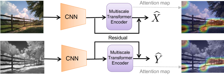
Figure 1: The proposed attention-based approach. A Siamese backbone CNN computes the feature maps of the input multimodal image patches that are passed through a Spatial Pyramid Pooling (SPP) layer [25]. A Transformer-Encoder aggregates the multiscale image embeddings. A residual connection bypasses the Encoder to facilitate end-to-end training. The attention heatmaps visualize the modality-invariant visual cues emphasized by the attention scheme.

In this work, we propose a novel approach for attention-based multimodal patch matching. The gist of our approach, shown in Fig. 1, is to apply attention using a multiscale Transformer-Encoder to aggregate multiscale image embeddings into a unified image descriptor. Multiscale feature maps allow the encoder to capture additional similarities between the multimodal patches. The descriptors are learned for both modalities by a weight-sharing Siamese network, which simultaneously learns the joint informative cues in the modalities of both patches. In particular, as depicted in the attention heatmaps visualized in Figs. 1 and 4, the modality-invariant informative visual cues correspond to the highest attention activations, computed by the encoder. Other image locations that are less task-informative show weak attention activations. To apply the Transformer-Encoder, we formulate the matching task as a sequence-to-one problem, where the inputs are multimodal feature maps flattened into sequences, and the outputs are adaptively aggregated embeddings. The spatial layout information of the image embeddings is induced by positional encoding. Due to the lack of pre-trained CNN backbones for multimodal patch matching, the backbone CNN has to be trained from scratch, starting from randomly initialized weights. This has become the de facto initialization scheme among other models in the task. We show that random initialization prevents the encoder from learning meaningful sequence aggregations at the beginning of the training process, hindering overall learning. To mitigate this issue, we propose adding a residual connection to the network bypassing the Transformer-Encoder, ultimately allowing end-to-end training of the proposed architecture from scratch.

Our approach is experimentally shown in Section IV to achieve the new SOTA multimodal matching accuracy on multiple datasets compared to the contemporary multisensor-specific descriptor learning schemes. Moreover, its applicability is further motivated by showing in Section IV-F, that when applied with SOTA general-purpose matching schemes, including CoAM [22], LoFTR [23] and SuperPoint [26], it outperforms these schemes in multisensor matching. Our results show that multisensor descriptor learning benefits from task-specific schemes such as ours, and motivates their use.

We highlight the following key contributions.

1. Introduction of a unique attention-based methodology for multimodal image patch matching. This method aggregates Siamese CNN feature maps using a multiscale Transformer-Encoder. To our knowledge, this represents the inaugural application of the Transformer-Encoder architecture to the task of multimodal image patch matching.

2. Proposal of a residual connection that bypasses the encoder, facilitating end-to-end training from scratch. This is pivotal given the common practice of random initialization and the absence of pre-trained backbones.

3. Demonstrated state-of-the-art (SOTA) performance of our method on contemporary multimodal image patch matching benchmarks, including VIS-NIR [27] and En et al. [9, 10]. Additionally, our method sets new SOTA standards on the single modality UBC Benchmark [28], underscoring the broad applicability of our approach.

4. Evidence that when our proposed multisensor image descriptors are combined with leading matching schemes [22, 23, 26], they surpass matching schemes that utilize general-purpose image descriptors trained on both RGB and multisensor datasets.

II Related work

II-A Shallow multisensor image matching

The matching of multi sensor images has been studied in a gamut of works. Earlier works, preceding contemporary CNN-based schemes, were based on unsupervised approaches, mostly based on deriving appearance-invariant image representations of multisensor images, that utilized salient image edges and contours. A robust image representation technique grounded in statistical methods was developed by Viola and Wells [29]. The mutual information between these statistical representations was fine-tuned to optimize motion parameters. An iterative, implicit similarity algorithm for global image alignment was devised by Keller et al. [30]. Leveraging gradient information, this approach identifies pixels with peak gradients in one image and optimizes the gradients at corresponding locations in the second image. This is done in relation to global parametric motion, without the need for explicit similarity measure optimization. Irani et al. introduced a hierarchical, coarse-to-fine strategy for estimating global parametric motion between multimodal images [31]. Using directional derivative magnitudes as a robust form of image representation, the correlation between these representations was iteratively maximized. This was achieved through the application of gradient ascent in a coarse-to-fine manner. Local modulality-invariant descriptors were derived by modifying the SIFT descriptor [32, 33]. Contrast-invariance was achieved by mapping the gradient orientations of interest points from $[0,2\pi)$ to $[0,\pi)$. However, Hasan et al. showed that such mappings decrease the accuracy of the matching [34]. They further modified SIFT [35] by thresholding gradient values to reduce the impact of strong edges. Enlarging the spatial window with additional sub-windows improved spatial resolution. Rather than using gradients, Aguilera et al. [36] employed histograms of contours and edges to avoid SIFT ambiguities in multimodal images. The dominant orientation was determined similarly. They later extended this approach by incorporating multi-oriented, multi-scale Log-Gabor filters [37]. Keller and Averbuch introduced an energy minimization approach to register multimodal images [38]. The alignment of the location of the gradient maxima is used as a robust matching criterion formulated as parametric optimization. The method iterates using one image’s intensity and initializing with the other’s gradient maxima. A coarse-to-fine scheme enables estimating global motion even with complex spatially-varying intensity transformations. This implicit matching criterion utilizes full spatial information without needing invariant representations. The technique is demonstrated by registering real multi-sensor images using affine and projective motion models. Geometric structure was used as an appearance-invariant representation by quantifying similarity through structural similarity measures. Shechtman et al. [39] introduced Self Similarity Matching (SSM), a geometric descriptor encoding local structure around feature points. This was done by correlating a central patch with all adjacent patches within a radius. Kim et al. [40] extended SSM with the Dense Adaptive Self-Correlation (DASC) descriptor. This computed a self-similarity measure via adaptive self-correlation between randomly sampled patches.

Ye et al. proposed a robust multimodal image registration method [41] to address nonlinear radiometric differences and geometric distortions between remote sensing images (optical, infrared, LiDAR, SAR). A novel Steerable Filters descriptor combining first- and second-order gradient information depicts discriminative structure features using a multi-scale strategy. Fast Normalized Cross-Correlation similarity measure using FFT and integral images improves efficiency. A coarse-to-fine system first conducts local coarse registration using interest points and geometric correction, utilizing image georeferencing. The proposed descriptor is robust to radiometric differences in fine registration, detecting control points by template matching. A robust feature matching method (R₂FD₂) for multimodal images was proposed by Zhu et. al [42]. It handles both differences in radiation and geometry. A repeatable feature detector (multichannel autocorrelation of log-Gabor) combines multichannel autocorrelation and log-Gabor wavelets to detect interest points with high repeatability and uniform distribution. A rotation-invariant descriptor (rotation-invariant maximum index map of log-Gabor) includes fast dominant orientation assignment and feature representation construction. A rotation-invariant maximum index map addresses rotation deformations. The descriptor incorporates this rotation-invariant map with the spatial configuration of DAISY to improve robustness to radiation and rotation differences. Zhou et al. applied deep learning to refine structure features and improve image matching [43]. The process involves extracting multi-oriented gradient features to represent the structure properties of images, then using a shallow pseudo-Siamese network to convolve the gradient feature maps in a multiscale manner. This results in multiscale convolutional gradient features (MCGFs), which are used for image matching via a fast template scheme. MCGFs can capture finer common features between SAR and optical images than traditional handcrafted structure features, and can also overcome some limitations of current deep learning-based matching methods. The performance of MCGFs was evaluated using two sets of SAR and optical images with different resolutions.

II-B CNN-based approaches for image matching

Deep learning techniques became the staple of computer vision and were applied to multimodal matching, showing SOTA performance. Jahrer et al.[13] introduced a Siamese CNN network for the metric learning of feature descriptors, outperforming classic hand-crafted descriptors such as SIFT [6]. Han et al.[15] added a metric learning network on top of a Siamese CNN, achieving SOTA results and also decreasing the size of the learned descriptors. Ofir et al. [44] propose a deep learning approach to align cross-spectral images using a learned descriptor. A feature-based method detects Harris corners and matches them using a patch-metric learned on top of a network trained on CIFAR-10. The approach achieves accurate sub-pixel alignment of cross-spectral images. Zagoruyko and Komodakis [14] explored multiple Siamese-based CNN architectures. The first is a 2-Channel architecture where the patches are concatenated channel-wise and are fed to a single CNN. The second is a Pseudo-Siamese CNN network with non-shared weights, and the last is a central surrounding architecture, in which two Siamese CNNs are jointly trained with different input resolutions to better capture multiresolution information. All methods presented promising results on the reported benchmarks. Aguilera et al.[27] extended those architectures to the multimodal case, outperforming previous approaches. Balntas et al. suggested a weight-sharing triplet CNN termed PN-Net [8], using image triplets consisting of two matching patches in addition to a non-matching one. A new loss was introduced to replace hard negative mining, by penalizing small $L_{2}$ distances between non-matching pairs and large $L_{2}$ distances between matching pair, forcing the network to always perform backpropagation using the hardest non-matching sample of each triplet. Aguilera et al. proposed a cross-spectral extension to the previous work, a weight-sharing quadruple network called Q-Net [9], utilizing two pairs of cross-spectral patches. The loss was extended to the quadruple case, mining both hard positive and hard negative samples at the same time. L2-Net [18] proposed by Tian et al. addressed an inherent problem in patch matching, where the number of negative samples is orders of magnitude larger than the positive samples, picking $n^{2}-n$ hard negative samples per batch with a minimum distance to the $n$ positive batch pairs. Mishchuk et al. proposed the HardNet extension [17] to L2-Net [18] using a hard negative sampling scheme, ensuring that the distance of the selected negative sample is minimal. Both approaches achieved SOTA performance on unimodal benchmarks. Wang et al. introduced a novel Exponential Loss function [12] forcing the network to learn more from both positive and negative hard samples than from easy ones. The scheme combines hard negative and positive mining inspired by Mishchuk et al.[17] and Simo et al.[16], respectively. Irshad et al. followed this line with the Twin-Net [19] approach, by proposing to mine twin negatives along with a dedicated Quad Loss, designed for single modality patches. In twin negatives mining, the first negative is mined as in Mishchuk et al.[17], and its closest negative is picked as the second negative. The Quad Loss then forces the descriptors of the chosen positive and anchor to be closer than the twin negatives descriptors, resulting in descriptors with a greater discriminatory power. Zhang and Rusinkiewicz [45] proposed an improved triplet loss formulation for feature learning, adaptively modifying the hard margin used to screen the hard negative. The authors suggest replacing the hard margin with a nonparametric soft margin, which is dynamically updated based on the cumulative distribution function of the triplets’ signed distances to the decision boundary.

En et al. proposed an approach to utilize both joint and modality-specific information within the image patches, by combining Siamese and Pseudo Siamese CNNs in a unified architecture dubbed TS-Net [10]. Ben-Baruch and Keller [11] introduced a similar hybrid framework fusing Siamese and Pseudo Siamese CNNs features through fully connected layers. Contrary to TS-Net [10], their approach calculated $L_{2}$-optimized patch descriptors essential for patch matching, and optimized the network using multiple auxiliary losses. These extensions have proven vital and have resulted in the performance of SOTA on various multimodal benchmarks. Quan et al. proposed the AFD-Net framework [46] consisting of three subnetworks, the first aggregates multilevel feature differences, the second extracts domain-invariant features from image patch pairs, while the final one infers matching labels. This approach computes a patch similarity score, rather than image embeddings. Thus, $\mathcal{O}(n^{2})$ forward passes of the network are required for matching two images containing $n$ image patches each, in contrast to $\mathcal{O}(n)$ forward passes in a descriptor learning approach such as ours.

II-C Transformer-based approaches in computer vision

The transformer architecture was introduced by Vaswani et al. [47] as a novel formulation of attention-based approaches, which allows encoding sequences without RNN layers such as LSTM and GRU. Transformers were first applied in Natural Language Processing tasks [48], and then proved successful in a variety of computer vision schemes [49, 50, 51, 52, 24]. Transformers, in contrast to convolution networks, are capable of aggregating long-range interactions between a sequence of input vectors. In computer vision, we can formulate the outputs of a backbone CNN as a sequence as in [50, 24, 51] and encode them using a Transformer encoder that aggregates spatial interactions (attention weights) between the activation map entries. Task-informative entries are numerically enhanced compared to noninformative ones. The Transformer architecture is composed of stacked layers of self-attention encoders and decoders attending the encoder outputs using a set of vectors denoted as queries. Using self-attention, the encoder produces a weighted average over the values of its inputs, such that the weights are produced dynamically using a similarity function between the inputs. Transformer-based encoders and decoders utilize multiple stacked multi-head Attention and feedforward layers. In contrast to the sequentially structured RNNs, the relative position and sequential order of the sequence elements are induced by positional encodings that are added to the Attention embeddings.

II-D Attention-based approaches for unimodal image matching

Attention-based approaches have recently been applied in unimodal, unconstrained image matching frameworks. SuperGlue [24] by Sarlin et al. studied feature matching using a graph neural network in combination with self- (intra-image) and cross- (inter-image) attention to leverage both the spatial relationships of the features and their visual appearance. Local features are extracted by CNN-based methods such as SuperPoint [26], or traditional descriptors like SIFT [6]. The SOLAR framework [53] by Ng et al. for image retrieval and descriptor learning utilizes SOSNet [54] for second-order similarity as a loss term and also takes advantage of second-order spatial relations between spatial features.

Wiles et al. introduced a spatial co-attention mechanism coined CoAM [22] for determining correspondences between image pairs with large differences in illumination, viewpoint, context, and material. This approach conditions on both images to implicitly account for their differences. It introduces two key components - a spatial co-attention module (CoAM) that conditions learned features on both images, and a distinctiveness score to pinpoint the most suitable matches. The LoFTR approach [23] by Sun et al. is of particular interest as it introduces an attention and Transformer-based local image feature matching approach that archived SOTA matching accuracy in unimodal images. The LoFTR technique initiates by establishing dense pixel-wise matches between images at a coarse scale, subsequently refining these matches at a more detailed scale. By employing self-attention and cross-attention layers within Transformers, LoFTR derives feature descriptors influenced by both images.

In contrast, we propose to combine a Siamese CNN for feature extraction with self-attention implemented by a multiscale Transformer-Encoder. while, LoFTR uses a single resolution scale at each network layer overlooking the multiscale structure of multisensor matching that is based on matching elongated edges and image structures, as shown in Section IV-G and Fig. 4. The use of a single resolution scale is appropriate in RGB images, where the higher scale (smaller) objects and image structures are captured similarly in all images up to appearance variations. Moreover, both the LoFTR [23] and CoAM [22] use cross-attention to compute image matching rather than descriptor learning, as in our approach. LoFTR’s Image matching is jointly applied to both images, implying that it computes the matching between two particular images, while our approach computes image descriptors separately for each image. This implies that when matching an input image $\mathbf{x}$ to a set of $n$ reference images $\left\{\mathbf{y}_{i}\right\}_{1}^{n}$, LoFTR has to be applied $n$ times for the tuples $\left\{\mathbf{x,y}_{i}\right\}_{1}^{n}$, while the proposed descriptor learning scheme has to applied just once to compute the descriptors for $\mathbf{x}$. We further demonstrate that our model can be trained end-to-end from scratch using the small training datasets available for multisensor matching, by using a novel residual connection, that circumvents the multiscale Transformer-Encoder. This allows the training signal to flow directly form the loss to the CNN layers in the first few training epochs. Compared to LoFTR [23], CoAM [22] and SuperGlue [24], our approach studies descriptor learning only and can be applied with any matching scheme such as RANSAC [20] and SuperGlue.

III Multiscale attention-based multimodal patch matching

We propose a novel attention-based approach for multimodal image patch matching by encoding Siamese CNN feature maps using the multiscale Transformer-Encoder architecture. We also introduce a residual connection bypassing the encoder, that is crucial for end-to-end training. We model the task as a sequence-to-one problem, where the inputs are multiscale feature maps of patches transformed into sequences, and the output is a learned feature descriptor. An overview of the proposed scheme is shown in Fig. 1.

Let $\{\mathbf{X},\mathbf{Y}\}\in\mathbb{R}^{H\times W\times C}$ be a pair of multimodal image patches. First, we compute the corresponding activation maps $\{\overline{\mathbf{X}},\overline{\mathbf{Y}}\}\in\mathbb{R}^{\overline{H}\times\overline{W}\times\overline{C}}$ using the Siamese CNN backbone. A spatial pyramid pooling layer (SPP) [25] is applied to $\{\overline{\mathbf{X}},\overline{\mathbf{Y}}\}$, to calculate a multiscale activation map $\{\mathbf{\widetilde{X}}_{k},\mathbf{\widetilde{Y}}_{k}\}\in\mathbb{R}^{\widetilde{H_{k}}\times\widetilde{W}_{k}\times\overline{C}}$, $k=1..K,$ as detailed in Section III-A. Each of $\{\mathbf{\widetilde{X}}_{k},\mathbf{\widetilde{Y}}_{k}\}$ is flattened into a sequence and aggregated into a single vector by the Transformer-Encoder, as in Section III-B. A fully connected layer finally maps the output representations into $\{\mathbf{\widehat{X}},\mathbf{\widehat{Y}}\}\in\mathbb{R}^{128}$. We also propose a novel residual connection described in Section III-C that bypasses the Transformer-Encoder and allows end-to-end training. The network is trained end-to-end using triplet loss [55] and a symmetric formulation of the HardNet approach [17] detailed in Section III-D.

III-A Backbone CNN

For every pair of multimodal image patches $\{\mathbf{X},\mathbf{Y}\}$, we apply a Siamese CNN to extract the feature maps $\{\overline{\mathbf{X}},\overline{\mathbf{Y}}\}$. The CNN architecture is described in Table I. We use the same backbones as previous works [12, 14], to experimentally exemplify the efficiency of the proposed attention-based scheme in Section IV. Each convolutional layer is followed by Batch Normalization and ReLU activation. We use an SPP layer [25] consisting of a four-level pyramid pooling, transforming the CNN feature maps into $K$ multiscale feature maps $\{\mathbf{\widetilde{X}}_{k},\mathbf{\widetilde{Y}}_{k}\}\in\mathbb{R}^{\widetilde{H_{k}}\times\widetilde{W}_{k}\times\overline{C}}$ such that $\mathbf{\widetilde{H}}_{k}$ and $\mathbf{\widetilde{W}}_{k}\in\{8,4,2,1\}$.

Layer	Output	Kernel	Stride	Pad	Dilation
Conv0	$64\times 64\times 32$	$3\times 3$	1	1	1
Conv1	$64\times 64\times 32$	$3\times 3$	1	1	1
Conv2	$31\times 31\times 64$	$3\times 3$	2	1	2
Conv3	$31\times 31\times 64$	$3\times 3$	1	1	1
Conv4	$29\times 29\times 128$	$3\times 3$	1	1	2
Conv5	$29\times 29\times 128$	$3\times 3$	1	1	1
Conv6	$29\times 29\times 128$	$3\times 3$	1	1	1
Conv7	$29\times 29\times 128$	$3\times 3$	1	1	1

TABLE I: The architecture of the Siamese CNN backbone.

III-B Multiscale Transformer-Encoder

The proposed weight-sharing multiscale Transformer-Encoder aggregates the $K$ multiscale outputs of the backbone CNN and SPP layer, and is illustrated in Fig. 2. The encoder has two layers, each consisting of two multi-head attention blocks. Given $K$ multiscale feature maps $\{\mathbf{\widetilde{X}}_{k},\mathbf{\widetilde{Y}}_{k}\}$, each map is spatially flattened into a sequence of size $\widetilde{H}_{k}\ast\widetilde{W}_{k}\times\overline{C}$.  Since the last SPP layer $\{\mathbf{\widetilde{X}}_{4},\mathbf{\widetilde{Y}}_{4}\}$ is of dimensions $\in\mathbb{R}^{1\times\overline{C}}$ there is no need for additional spatial pooling, and it is passed as is, and concatenated in the output vecror.

We assign a learnable embedding to each sequence whose corresponding output is the aggregated result, the same as [CLS] token used in BERT [48]. In order to induce spatial information to the permutation-invariant Transformer encoder, we learn separable 2D positional encodings. The encoding is learned separately for the $X$ and $Y$ axes to reduce the number of learned parameters and are denoted as $\mathbf{E}_{X}\in\mathbb{R}^{\widetilde{H}_{k}\times\frac{\overline{C}}{2}}$ and $\mathbf{E}_{Y}\in\mathbb{R}^{\widetilde{W}_{k}\times\frac{\overline{C}}{2}}$ respectively. The final 2D positional encoding $\mathbf{E}_{i,j}\in\mathbb{R}^{\overline{C}}$ is given by:

$$\mathbf{E}_{i,j}=\begin{bmatrix}\mathbf{E}_{X}^{j}\\ \mathbf{E}_{Y}^{i}\end{bmatrix},\left[i,j\right]\in\left[1...\widetilde{H_{k}},1...\widetilde{W}_{k}\right]$$ (1)

Positional encodings are then spatially flattened into a sequence of size $\widetilde{H}_{k}\ast\widetilde{W}_{k}\times\overline{C}$ and summed with the feature map sequences $\{\mathbf{\widetilde{X}}_{k},\mathbf{\widetilde{Y}}_{k}\}$. The Transformer-Encoder is then applied to the enriched feature map sequences to produce $K$ aggregations, denoted $\left\{\mathbf{O}_{k}^{X},\mathbf{O}_{k}^{Y}\right\}$. $\left\{\mathbf{O}_{k}^{X}\right\}$ and $\left\{\mathbf{O}_{k}^{Y}\right\}$ are concatenated separately into two vectors of dimension $\mathbb{R}^{4\overline{C}}$, together with the feature map of the residual connections $\left\{\mathbf{\widetilde{X}}_{8},\mathbf{\widetilde{Y}}_{8}\right\}\in\mathbb{R}^{8\times 8\times\overline{C}}$, as discussed in Section III-C. Then each of the two concatenated embeddings is passed through an FC layer and $L_{2}$ normalized.

III-C The residual connection

It is common to apply attention layers to pre-trained backbone CNNs that are kept frozen during the training process, allowing the Transformer-Encoder to train based on meaningful feature representations computed by the backbone. In contrast, in multimodal matching, the backbone has to be trained end-to-end from scratch, due to the absence of pre-trained weights for the task. Thus, at the beginning of the training, until the CNN learns to extract useful feature maps, the encoder does not manage to learn meaningful sequence aggregations either, hindering the overall learning. Hence, we propose to resolve this issue by passing the pooled feature map $\left\{\mathbf{\widetilde{X}}_{8},\mathbf{\widetilde{Y}}_{8}\right\}\in\mathbb{R}^{8\times 8\times\overline{C}}$, having the largest spatial support, directly to the output layer using a residual connection. The residual connection circumvents the encoder, adding a vital learning signal allowing end-to-end training from scratch. The residual feature map is flattened into a vector $\in\mathbb{R}^{8\cdot 8\cdot\overline{C}}$ and concatenated into the output vector. Note that in practice, the output of the SPP layer $\{\mathbf{\widetilde{X}}_{4},\mathbf{\widetilde{Y}}_{4}\}$ $\in\mathbb{R}^{1\times\overline{C}}$ is also a residual connection (Fig. 2), but due to the intensive pooling, down to $1\times 1,$ the embedding is too diluted and does not allow convergence. Thus, as exemplified in Table VI, our architecture cannot be trained from scratch without the proposed residual connection. Finally, the concatenated output is mapped by a fully connected layer $FC$ that produces feature descriptors for each pair of patches, denoted $\{\mathbf{\widehat{X}},\mathbf{\widehat{Y}}\}\in\mathbb{R}^{128}$.

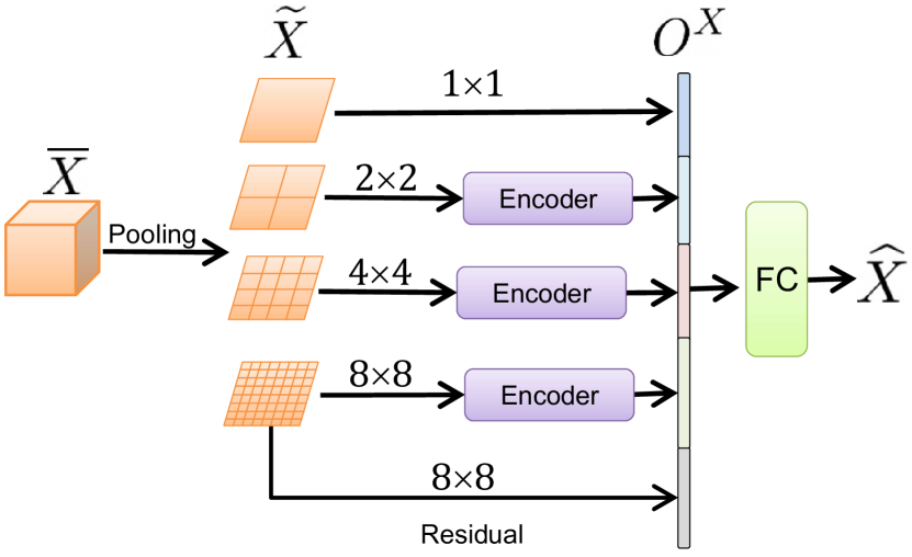
Figure 2: The proposed multiscale Transformer-Encoder architecture. $\overline{\mathbf{X}}$ is a feature map computed by the backbone CNN, and pooled into four multiscale feature maps $\mathbf{\widetilde{X}}_{k}$ by a SPP layer [25]. The Transformer-Encoder aggregates the pooled maps $\mathbf{\widetilde{X}}_{k}$ along with their positional encodings, and the aggregations $\mathbf{O}_{k}^{X}\in\mathbb{R}^{128}$ are concatenated alongside the residual connection.

III-D Symmetric triplet loss

The proposed network is trained by applying the Triplet Loss [55] to the outputs $\{\mathbf{\widehat{X}},\mathbf{\widehat{Y}}\}$:

$$L_{t}\left(a_{i},p_{j},n_{k}\right)=\sum_{n,j,k}^{N}max(0,m+d(a_{i},p_{j})-d(a_{i},n_{k}))$$ (2)

where $a_{i},p_{j}$ and $n_{k}$ are triplets of the anchor, positive, and negative samples, respectively. $m$ is a margin, and $d$ is the Euclidean distance. Given a training batch of $B$ embeddings $\{\mathbf{\widehat{X}}_{i},\mathbf{\widehat{Y}}_{i}\}_{1}^{B}$, for each entry $i$ we have $a_{i}=\mathbf{\widehat{X}}_{i},$ $p_{j}=\mathbf{\widehat{Y}}_{i}$ and $n_{k}$ and is a sample $\mathbf{\widehat{Y}}_{j}\in\{\mathbf{\widehat{Y}}_{i}\}_{1}^{B},j\neq i$. Initially, $\mathbf{\widehat{Y}}_{j}$ is chosen randomly, and then we switch to hard mining. As the hard negative $n_{k}$ is dynamically chosen within each batch following the HardNet approach [17], we utilize the symmetry between the channels $\mathbf{\widehat{X}}_{i}$ and $\mathbf{\widehat{Y}}_{i}$ and train the network using a symmetrized formulation of Eq. 2 as follows:

$$L_{t}^{s}\left(a_{i},p_{j},n_{k},n_{k^{\prime}}\right)=L_{t}\left(a_{i},p_{j},n_{k}\right)+L_{t}\left(p_{j},a_{i},n_{k^{\prime}}\right)$$ (3)

We used $m=1$ which is a common choice for the margin that also worked well in previous works. We also experimented using other values, but the performance did not improve. We chose $d$ as the Euclidean distance function to be able to utilize efficient large-scale K nearest-neighbor search schemes for matching descriptors in $L_{2}$ spaces [56].

IV Experimental Results

We evaluated the proposed scheme using multiple contemporary multimodal patch matching datasets. We use their publicly available setups that provide a deterministic generation of matching and non-matching train and validation patches. This allows us to apply a repeatable experimental setup that is shared and utilized by us and the SOTA schemes against which we compare. We also demonstrate the generality of our proposal by evaluating it on the UBC benchmark [28], a general single-modality benchmark for patch matching that was used in previous work. We measure our performance using the false positive rate at 95% recall (FPR95), where a smaller FPR95 score is better.

IV-A Datasets

The VIS-NIR Benchmark [27] is a cross-spectral image patch matching benchmark consisting of over 1.6 million RGB and Near-Infrared (NIR) patch pairs of size $64\times 64$. The benchmark was collected by Aguilera et al. [27, 9] from the public VIS-NIR scene dataset. Half of the patches are matching pairs, and half are non-matching pairs chosen at random. A public domain code by Aguilera et al. allows to deterministically recreate the training and test sets, and was used by all schemes we compare against. The En et al. benchmark [10] consists of three different multimodal datasets sampled on a uniform grid layout, with a corresponding public domain code: VeDAI [57], consisting of vehicles in aerial imagery, CUHK [58], consisting of faces and face sketch pairs, and VIS-NIR [27]. Following the setup of En et al. [10], 70% of the data is used for training, 10% for validation and 20% for testing.

The UBC benchmark [28], also known as the Brown benchmark, is a single-mode data set consisting of image pairs sampled from 3D reconstructions. The benchmark consists of three subsets: Liberty, Notredame, and Yosemite, consisting of 450K, 468K, and 634K patches, respectively. Patches were extracted using Difference of Gaussian [6] or Harris corner detector [59]. Half of the patches, with the same 3D point, are matching pairs, and the rest are non-matching pairs. Following [28, 18, 14, 17] we iteratively train on one subset and test on 100k pairs of the other subsets.

IV-B Training

We use PyTorch [60] with three NVIDIA GeForce GTX 1080 Ti GPUs. The networks are randomly initialized from a normal distribution and optimized using Adam [61] with an initial learning rate of 0.1. A warm-up learning rate scheduler [62] was used for eight epochs and then replaced by a scheduler that reduced the learning rate by a factor of 10 for every plateau of three epochs. The architecture was trained for 70 epochs using batches of size 48. The patches were mean-centered and normalized, and basic augmentations of horizontal flips and rotations were applied. The architecture is trained with random negatives until there is no loss decrease for three epochs. We then start mining hard negative samples using Mishchuk et al. technique [17]. Our code is shared here: Code.

IV-C VIS-NIR Benchmark

Method	Field	Forest	Indoor	Mountain	Old building	Street	Urban	Water	Mean
Handcrafted descriptor methods
SIFT [6]	39.44	11.39	10.13	28.63	19.69	31.14	10.85	40.33	23.95
MI-SIFT [63]	34.01	22.75	12.77	22.05	15.99	25.24	17.44	32.33	24.42
LGHD [64]	16.52	3.78	7.91	10.66	7.91	6.55	7.21	12.76	9.16
Learning-based methods
Siamese [27]	15.79	10.76	11.6	11.15	5.27	7.51	4.6	10.21	9.61
Pseudo Siamese [27]	17.01	9.82	11.17	11.86	6.75	8.25	5.65	12.04	10.32
2-Channel [27]	9.96	0.12	4.4	8.89	2.3	2.18	1.58	6.4	4.47
PN-Net [8]	20.09	3.27	6.36	11.53	5.19	5.62	3.31	10.72	8.26
Q-Net [9]	17.01	2.70	6.16	9.61	4.61	3.99	2.83	8.44	6.86
TS-Net [10]	25.45	31.44	33.96	21.46	22.82	21.09	21.9	21.02	24.89
SCFDM [65]	7.91	0.87	3.93	5.07	2.27	2.22	0.85	4.75	3.48
L2-Net [18]	16.77	0.76	2.07	5.98	1.89	2.83	0.62	11.11	5.25
HardNet [17]	10.89	0.22	1.87	3.09	1.32	1.30	1.19	2.54	2.80
Exp-TLoss [12]	5.55	0.24	2.30	1.51	1.45	2.15	1.44	1.95	2.07
D-Hybrid-CL [11]	4.4	0.20	2.48	1.50	1.19	1.93	0.78	1.56	1.7
Ours	4.22	0.13	1.48	1.03	1.06	1.03	0.9	1.9	1.44

TABLE II: Patch matching results evaluated on the VIS-NIR Benchmark [27]. The score is given in terms of FPR95.

To demonstrate the effectiveness of our approach in the multimodal image patch matching task, we compare it with 14 state-of-the-art methods, using the same setup as Aguilera et al. [27] and [10, 9, 11]. The Country category is divided into 80% and 20% for training and validation, respectively. The rest of the categories are used for testing. The results are shown in Table II. We compare our proposal to both handcrafted descriptors [6, 63, 64] and state-of-the-art deep learning methods. We quote the results reported by [12, 11] on this benchmark.

For the handcrafted descriptors [6, 63, 64] we used their publicly available code. As in previous works, such approaches are outperformed by learning-based methods due to their inability to capture high-level semantic information. PN-Net [8], L2-Net [18], HardNet [17] and Exp-TLoss [12] are single-mode general-purpose schemes that were applied to the VIS-NIR benchmark by Wang et al.[12]. These approaches, which are based on a Siamese CNN architecture, the same as the proposed scheme, generalized well to the multimodal case. Aguilera et al.’s three proposals [27] of vanilla Siamese CNN, Pseudo Siamese CNN, 2-Channel CNN, as well as SCFDM [65] and D-Hybrid-CL [11] were specifically designed for multimodal image patch matching and were tested on the VIS-NIR benchmark. The SOLAR framework training code for local descriptor learning [53] was not made public, and the publicly available pre-trained model performed poorly in the multisensor dataset. So we avoided reporting its results due to lack of insights. Our proposed scheme outperforms all previous approaches, achieving a new SOTA on this benchmark. In particular, it surpasses the previous SOTA Exp-TLoss [12] by 43% and D-Hybrid-CL [11] by 18%. Both methods are based on the same backbone CNN and SPP layer. Therefore, we attribute the improved performance to the proposed attention-based inference, compared to previous schemes [12, 11] that are limited to multiscale SPP-based inference without spatial attention-based aggregation.

IV-D En et al. Benchmark

We apply our approach to this multimodal benchmark following En et al.’s [10] publicly available setup and compare with ten state-of-the-art methods, both handcrafted [6, 63, 64] and learning-based [27, 9, 10, 11]. The results are reported in Table III. We quote the results of previous schemes reported by [10, 11] on this benchmark.

On the VeDAI dataset, both 2-Channel [27], Hybrid [11] variants and our approach achieve zero error. On CUHK, our approach achieves the same performance as Hybrid-CE [11]. CUHK is a dataset composed of pairs of faces along with their face sketches. In this case, where the features are relatively limited and spatially close to each other, it seems that self-attention over the feature maps might not capture additional information. However, we established a new SOTA in the VIS-NIR data set, improving it by 93%.

Method	VeDAI	CUHK	VIS-NIR
Handcrafted descriptor methods
SIFT[6]	42.74	5.87	32.53
MI-SIFT [63]	11.33	7.34	27.71
LGHD[64]	1.31	0.65	10.76
Learning-based methods
Siamese[27]	0.84	3.38	13.17
Pseudo Siamese[27]	1.37	3.7	15.6
2-Channel[27]	0	0.39	11.32
Q-Net[9]	0.78	0.9	22.5
TS-Net[10]	0.45	2.77	11.86
Hybrid-CE [11]	0	0.05	3.66
Hybrid-CL [11]	0	0.1	3.41
Ours	0, $\sigma=0$	0.05	1.76
Ours FPR99	0, $\sigma=0$	-	-

TABLE III: Patch matching results evaluated on En et al. Benchmark [10] consisting of three multimodal datasets sampled on a uniform grid layout. The score is given in terms of FPR95. On the VeDAI dataset, we performed a stricter evaluation using FPR99 and reported the standard deviation out of 10 tests.

IV-E UBC Benchmark

Method	Training	NOT	YOS	LIB	YOS	LIB	NOT	Mean
	Testing	LIB		NOT		YOS
SIFT [6]		29.84		22.53		27.29
MatchNet [15]		7.04	11.47	3.82	5.65	11.60	8.70	8.05
TL+AS+GOR [66]		1.95	5.40	4.80	5.15	6.45	2.38	4.36
L2-Net [18]		3.64	5.29	1.15	1.62	4.43	3.30	3.23
CS L2-Net [18]		2.55	4.24	0.87	1.39	3.81	2.84	2.61
L2-Net [18]		2.36	4.70	0.72	1.29	2.57	1.71	2.22
CS L2-Net [18]		1.71	3.87	0.56	1.09	2.07	1.30	1.76
Scale aware [67]		0.68	2.51	1.79	1.64	2.96	1.02	1.64
HardNet [17]		0.53	1.96	1.49	1.84	2.51	0.78	1.51
Twin-Net [19]		1.19	2.12	0.41	0.69	1.58	1.62	1.27
Exp-TLoss [12]		0.47	1.32	1.16	1.10	2.01	0.67	1.12
Ours		0.35	0.91	1.31	0.85	1.58	0.41	0.9

TABLE IV: Patch matching results evaluated on the UBC Benchmark [28]. Score is given in terms of FPR95.
LIB: Liberty, NOT: Notredame, YOS: Yosemite.

To illustrate the general applicability of our approach, we compare it with 11 state-of-the-art methods using the popular single modality UBC Benchmark [28], and the publicly available setup and evaluation code , that was used by all the schemes we compare against. The results are presented in Table IV. We quote the previous results reported on this benchmark by [12, 19].

Our approach achieved a new SOTA performance when trained on the Liberty and Yosemite datasets, surpassing the previous SOTA by 24%. When trained on Notredame our approach is slightly outperformed by CS L2-Net [18] and Twin-Net [19]. We suspect that it is due to the significant geometric deformations in Notredame, degrading the feature maps extracted by our Siamese CNN. Notredame also consists of some extremely hard samples that Twin-Net [19] might be able to mine better using its improved hard samples mining scheme.

IV-F Keypoints matching accuracy

The proposed multimodal descriptor can also serve as a more accurate drop-in replacement for multimodal keypoint description in contemporary image matching algorithms such as CoAM [22], LoFTR [23], and SuperPoint [26], which is the detector and descriptor used in SuperGlue [24]. Hence, we applied SuperGlue [24] scheme using SuperPoint [26] and the proposed multisensor descriptors. We examine the effect of our method on the VIS-NIR dataset [27]. Following similar experiments by Ben Baruch et al. [11] we define an inlier as a matched pair of keypoints with a maximal matching error of 5 pixels. We extract the top 200 keypoints detected by each method, to compute the corresponding descriptors using our method, and report the mean number of inliers, outliers, and pixel distance error in Table V. Additional qualitative visualizations are shown in Figure 3. Our method improves the SuperPoint [26] inliers number by 7%, and reduces outliers and distance error by 27% and 90%, respectively. Significant improvement is also shown for CoAM [22], with a 65% reduction of the distance error. LoFTR [23] is the only method whose gain is less significant. In particular, comparing the accuracy of all matching schemes without using our approach shows that LoFTR is significantly more accurate, reducing the matching error by 83% and 92%, respectively. Hence, the use of our more accurate descriptor improves its results but not significantly. We attribute this to LoFTR’s architecture using a Transformer with a global receptive field.

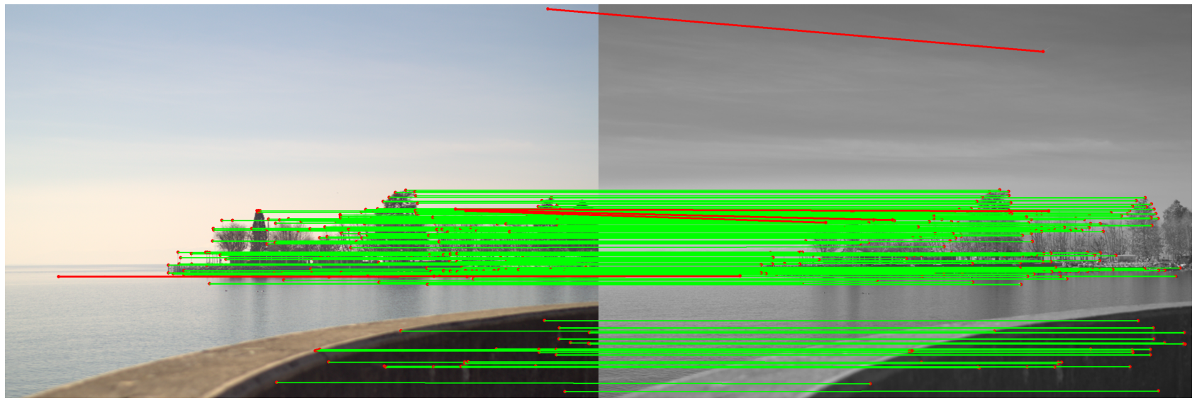
(a) SuperPoint

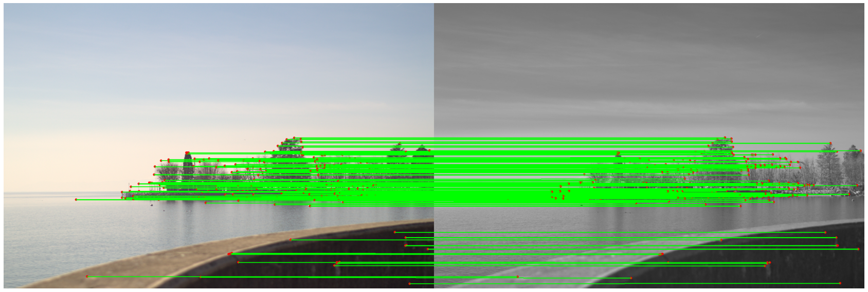
(b) SuperPoint+Ours

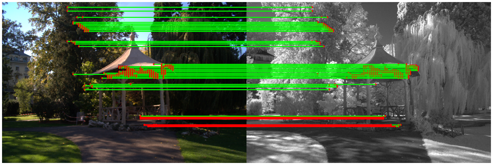
(c) CoAM

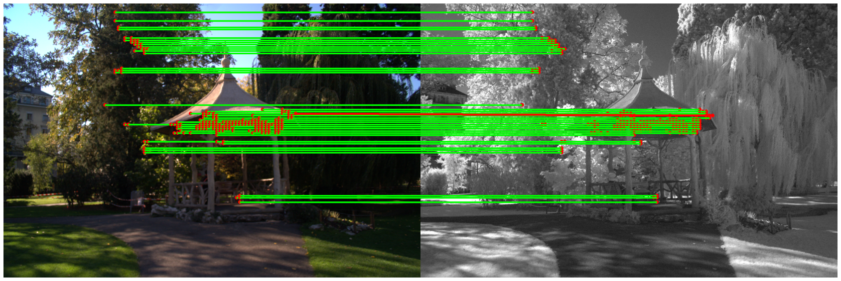
(d) CoAM+Ours

Figure 3: Keypoints matching visualizations of SuperPoint [26] in 3a-3b and CoAM [22] in 3c-3d with and without using the proposed scheme, on the VIS-NIR Benchmark [27]. Inliers are marked in green and outliers in red. Our method reduces the number of outliers and produces more accurate results.

Method	Inliers	Outliers	Matching Error $\bigl{[}pixels\bigr{]}$
SuperPoint[26]	160	40	140
SuperPoint[26] + Ours	171	29	14
CoAM[22]	189	11	57
CoAM[22] + Ours	190	10	20
LoFTR[23]	192	8	12
LoFTR[23] + Ours	189	7	10

TABLE V: The matching accuracy of SOTA matching schemes using the proposed multimodal image descriptor. We compare to applying the matching schemes with the SuperPoint [26] SOTA descriptor. We report the mean number of inliers, outliers, and matching error (in pixels) on the VIS-NIR dataset [27]. The inliers are defined as matched keypoints with a distance of less than 5 pixels [11].

IV-G Attention maps

We further study the Transformer-Encoder self-attention mechanism by visualizing the attention weights as heatmaps. This allows to analyze the visual cues the encoder pays attention to. We show the attention heatmaps of four matching RGB and NIR pairs taken from the VIS-NIR Benchmark [27], originated from different scenes. The heatmaps are generated by upsampling the attention weights of the last encoder layer.

The resulting attention maps are presented in Fig. 4, showing that the encoder learns to pay more attention to locations of modality-invariant features, paying more attention to locations consisting of object blobs or their distinctive corners and edges. In the first pair 4a, the encoder summarizes the scene well by paying attention to both the bigger traffic sign in the middle and the second, smaller one in the background. In the second pair 4b, the encoder attends to the distinctively shaped tree on the left, as well as the house corner, which is a good modality-invariant feature. The third pair 4c contains two small houses, and the encoder chooses to attend to both, also paying some attention to the grass fields in the foreground. In the fourth pair 4d, the encoder catches and attends the car in the middle of the scenes along with parts of the background house, but misses the black motorbike in the NIR image, probably due to occlusion in the NIR image.

	RGB	NIR
(a)
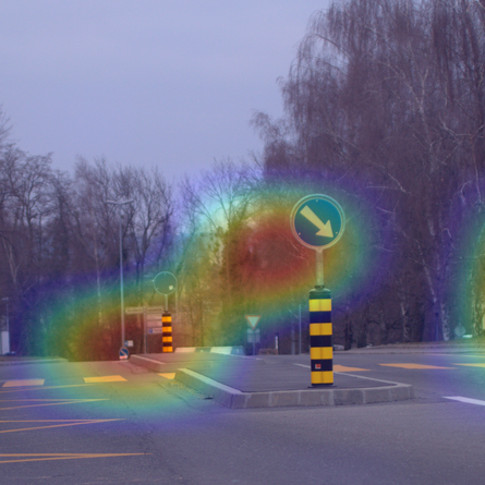
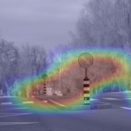
(b)
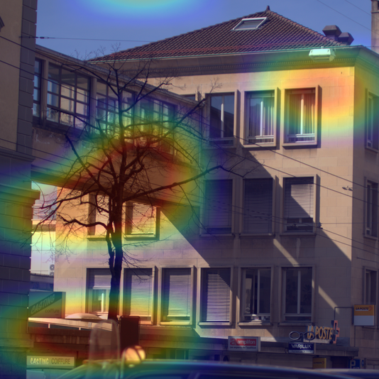
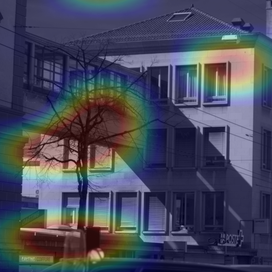
(c)
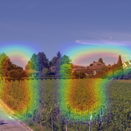
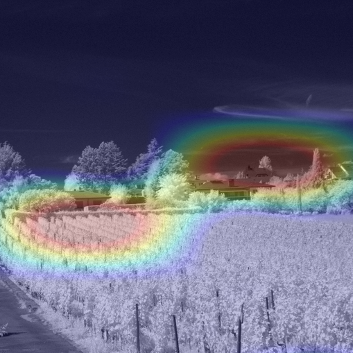
(d)

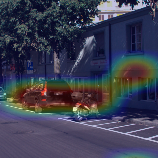
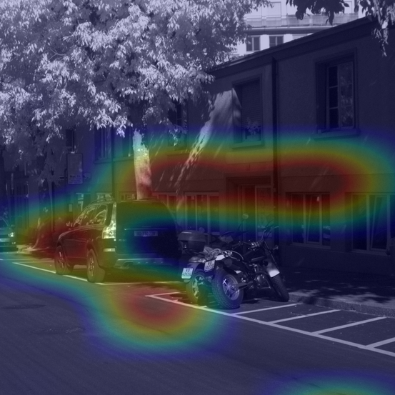
Figure 4: Attention heatmaps visualizing the Transformer-Encoder attention weights. The presented heatmaps show corresponding multimodal RGB and NIR images taken from various scenes of the VIS-NIR Benchmark [27].

IV-H Ablation study

CNN	Transformer	Attention		Residual	SPP	VIS-NIR
		Layers	Heads
Siamese	-	-	-	-	+	1.77
Siamese	-	-	-	-	-	1.83
Siamese	Encoder	4	2	+	+	1.5
Siamese	Encoder	2	4	+	+	1.59
Siamese	Encoder+ Decoder	2	2	+	+	1.66
Pseudo Siamese	Encoder	2	2	+	+	2.03
Siamese	Encoder	2	2	-	+	DIV
Siamese	Encoder	2	2	+	+	1.44

TABLE VI: Ablation results evaluated on the VIS-NIR Benchmark [27]. Score is given in terms of FPR95. DIV implies that the model diverged and was not able to learn.

To better understand the contribution of each component in our proposal, we experiment with modifying one component or related parameter at a time and measuring its impact. The experiments were performed on the VIS-NIR Benchmark [27], and are reported at Table VI. We first evaluate the impact of the Transformer-Encoder. When the transformer is removed and the rest of the architecture is intact, it is shown that the addition of the transformer provides a 23% improvement. Removing also the SPP as well as the Transformer results in even a greater error. Performance is not improved by adding encoder layers or heads, nor by adding a Transformer-Decoder on top of the encoder, which degrades performance by 14%, probably due to overfitting. A CNN of unshared weights, coined Pseudo-Siamese CNN and used in previous SOTA approaches [27, 11], ends up with inferior performance compared to the Siamese CNN, illustrating the importance of weight sharing. An additional observation is the significance of the residual connection, as without it the architecture cannot be trained end-to-end from scratch and the training diverges.

We further study the SPP layer impact. It is shown in Table VII that a four-level SPP yields the best results. Three levels degrade performance, as the $8\times 8$ layer was shown to contain valuable information for the model, and an additional level also degrades performance, illustrating that the additional low-resolution layer is insignificant. A reduced batch size was used due to memory constraints imposed by the $16\times 16$ level.

Pyramid levels	VIS-NIR
$4\times 4,2\times 2,1\times 1$	1.75
$8\times 8,4\times 4,2\times 2,1\times 1$	1.6
$16\times 16,8\times 8,4\times 4,2\times 2,1\times 1$	1.65

TABLE VII: SPP levels ablation results evaluated on the VIS-NIR Benchmark [27]. The score is given in terms of FPR95. Due to memory constraints, a smaller batch size was used.

Dimensions	Type	VIS-NIR
-	-	1.63
1D	Fixed	1.54
	Learned	1.58
2D	Fixed	1.62
	Learned	1.44

TABLE VIII: Positional encoding ablation results evaluated on the VIS-NIR Benchmark [27]. Score is given in terms of FPR95.

We also measure the impact of the different formulations of positional encoding in Table VIII, where we evaluated fixed and learned 1D and 2D positional encodings, following Parmar et al. [52] and Eq. 1. It follows that learning a 2D positional encoding yields the best performance, implying that the encoder benefits from utilizing the original 2D spatial layout of the features.

The embedding dimension used by the network was studied in Table IX by training the network from scratch using multiple dimensions. A larger embedding dimension can improve the network’s capacity, but can also lead to overfitting. The results in Table IX show that $\mathbb{R}^{128}$ is the sweet spot, as the model does not benefit from a larger descriptor size and its performance is degraded by using a smaller descriptor.

Dimension	VIS-NIR
64	1.93
128	1.44
256	1.45

TABLE IX: Descriptor size ablation results evaluated on the VIS-NIR Benchmark [27]. The score is given in terms of FPR95.

V Conclusions

In this paper, we presented a novel approach for performing multimodal image patch matching using a Transformer-Encoder on top of Siamese CNN multiscale feature maps, utilizing long-range feature interactions as well as modality-invariant feature aggregations. We also introduced a residual connection, which has been shown to be essential for training Transformer-based networks from scratch. The proposed scheme achieves new SOTA performance when applied to contemporary multimodal patch matching benchmarks and the popular single modality UBC Benchmark, illustrating its generality.

References

- [1] A. Sotiras, C. Davatzikos, and N. Paragios, “Deformable medical image registration: A survey,” IEEE Transactions on Medical Imaging, vol. 32, no. 7, pp. 1153–1190, 2013.
- [2] M. Irani and P. Anandan, “Robust multi-sensor image alignment,” in Proceedings of the IEEE International Conference on Computer Vision (ICCV), 1998, pp. 959–966.
- [3] J. Chen and J. Tian, “Real-time multi-modal rigid registration based on a novel symmetric-sift descriptor,” Progress in Natural Science, vol. 19, p. 643–651, 05 2009.
- [4] M. T. Hossain, G. Lv, S. W. Teng, G. Lu, and M. Lackmann, “Improved symmetric-SIFT for multi-modal image registration,” in Proceedings of the 2011 International Conference on Digital Image Computing: Techniques and Applications, ser. DICTA ’11. USA: IEEE Computer Society, 2011, p. 197–202.
- [5] C. Aguilera, F. Barrera, F. Lumbreras, A. D. Sappa, and R. Toledo, “Multispectral image feature points,” Sensors, vol. 12, no. 9, pp. 12 661–12 672, 2012.
- [6] D. G. Lowe, “Distinctive image features from scale-invariant keypoints,” International Journal of Computer Vision, vol. 60, no. 2, p. 91–110, Nov. 2004.
- [7] H. Bay, A. Ess, T. Tuytelaars, and L. Van Gool, “Speeded-up robust features (SURF),” Computer Vision and Image Understanding, vol. 110, no. 3, p. 346–359, Jun. 2008.
- [8] V. Balntas, E. Johns, L. Tang, and K. Mikolajczyk, “PN-Net: conjoined triple deep network for learning local image descriptors,” CoRR, vol. abs/1601.05030, 2016.
- [9] C. A. Aguilera, A. D. Sappa, C. Aguilera, and R. Toledo, “Cross-spectral local descriptors via quadruplet network,” Sensors, vol. 17, no. 4, 2017.
- [10] S. En, A. Lechervy, and F. Jurie, “Ts-net: Combining modality specific and common features for multimodal patch matching,” in IEEE International Conference on Image Processing (ICIP), 2018, pp. 3024–3028.
- [11] E. B. Baruch and Y. Keller, “Joint detection and matching of feature points in multimodal images,” IEEE Transactions on Pattern Analysis and Machine Intelligence, vol. 44, no. 10, pp. 6585–6593, 2022.
- [12] S. Wang, Y. Li, X. Liang, D. Quan, B. Yang, S. Wei, and L. Jiao, “Better and faster: Exponential loss for image patch matching,” in Proceedings of the IEEE International Conference on Computer Vision (ICCV), Oct. 2019.
- [13] M. Jahrer, M. Grabner, and H. Bischof, “Learned local descriptors for recognition and matching,” in Proceedings of the Computer Vision Winter Workshop, 2008, pp. 39–46.
- [14] S. Zagoruyko and N. Komodakis, “Learning to compare image patches via convolutional neural networks,” in Proceedings of the IEEE/CVF Conference on Computer Vision and Pattern Recognition (CVPR), 2015, pp. 4353–4361.
- [15] Xufeng Han, T. Leung, Y. Jia, R. Sukthankar, and A. C. Berg, “Matchnet: Unifying feature and metric learning for patch-based matching,” in Proceedings of the IEEE/CVF Conference on Computer Vision and Pattern Recognition (CVPR), 2015, pp. 3279–3286.
- [16] E. Simo-Serra, E. Trulls, L. Ferraz, I. Kokkinos, P. Fua, and F. Moreno-Noguer, “Discriminative learning of deep convolutional feature point descriptors,” in Proceedings of the IEEE International Conference on Computer Vision (ICCV), December 2015.
- [17] A. Mishchuk, D. Mishkin, F. Radenović, and J. Matas, “Working hard to know your neighbor’s margins: Local descriptor learning loss,” in Advances in Neural Information Processing Systems (NIPS), 2017.
- [18] Y. Tian, B. Fan, and F. Wu, “L2-net: Deep learning of discriminative patch descriptor in euclidean space,” in Proceedings of the IEEE/CVF Conference on Computer Vision and Pattern Recognition (CVPR), 2017, pp. 6128–6136.
- [19] A. Irshad, R. Hafiz, M. Ali, M. Faisal, Y. Cho, and J. Seo, “Twin-net descriptor: Twin negative mining with quad loss for patch-based matching,” IEEE Access, vol. 7, pp. 136 062–136 072, 2019.
- [20] M. Fischler and R. Bolles, “Random sample consensus: A paradigm for model fitting with applications to image analysis and automated cartography,” Communications of the ACM, vol. 24, no. 6, pp. 381–395, 1981.
- [21] D. Baráth, J. Noskova, M. Ivashechkin, and J. Matas, “Magsac++, a fast, reliable and accurate robust estimator,” in Proceedings of the IEEE/CVF Conference on Computer Vision and Pattern Recognition (CVPR), 2020, pp. 1301–1309.
- [22] O. Wiles, S. Ehrhardt, and A. Zisserman, “Co-attention for conditioned image matching,” Proceedings of the IEEE/CVF Conference on Computer Vision and Pattern Recognition (CVPR), pp. 15 915–15 924, 2021.
- [23] J. Sun, Z. Shen, Y. Wang, H. Bao, and X. Zhou, “LoFTR: Detector-free local feature matching with transformers,” Proceedings of the IEEE/CVF Conference on Computer Vision and Pattern Recognition (CVPR), pp. 8918–8927, 2021.
- [24] P.-E. Sarlin, D. DeTone, T. Malisiewicz, and A. Rabinovich, “Superglue: Learning feature matching with graph neural networks,” in Proceedings of the IEEE/CVF Conference on Computer Vision and Pattern Recognition (CVPR), June 2020.
- [25] K. He, X. Zhang, S. Ren, and J. Sun, “Spatial pyramid pooling in deep convolutional networks for visual recognition,” IEEE Transactions on Pattern Analysis and Machine Intelligence, vol. 37, no. 9, pp. 1904–1916, 2015.
- [26] D. DeTone, T. Malisiewicz, and A. Rabinovich, “Superpoint: Self-supervised interest point detection and description,” IEEE Conference on Computer Vision and Pattern Recognition Workshops (CVPRW), pp. 337–33 712, 2018.
- [27] C. A. Aguilera, F. J. Aguilera, A. D. Sappa, C. Aguilera, and R. Toledo, “Learning cross-spectral similarity measures with deep convolutional neural networks,” in IEEE Conference on Computer Vision and Pattern Recognition Workshops (CVPRW), 2016, pp. 267–275.
- [28] M. Brown, G. Hua, and S. Winder, “Discriminative learning of local image descriptors,” IEEE Transactions on Pattern Analysis and Machine Intelligence, vol. 33, no. 1, pp. 43–57, 2011.
- [29] P. Viola and W. M. Wells, III, “Alignment by maximization of mutual information,” International Journal of Computer Vision, vol. 24, no. 2, pp. 137–154, Sep. 1997.
- [30] Y. Keller and A. Averbuch, “Multisensor image registration via implicit similarity,” IEEE Transactions on Pattern Analysis and Machine Intelligence, vol. 28, no. 5, pp. 794–801, 2006.
- [31] M. Irani and P. Anandan, “Robust multi-sensor image alignment,” in Proceedings of the IEEE International Conference on Computer Vision (ICCV). IEEE, 1998, pp. 959–966.
- [32] J. Chen and J. Tian, “Real-time multi-modal rigid registration based on a novel symmetric-SIFT descriptor,” Progress in Natural Science, vol. 19, no. 5, pp. 643–651, 2009.
- [33] R. Ma, J. Chen, and Z. Su, “MI-SIFT: Mirror and inversion invariant generalization for SIFT descriptor,” in Proceedings of the ACM International Conference on Image and Video Retrieval, ser. CIVR ’10, 2010, pp. 228–235.
- [34] M. T. Hossain, G. Lv, S. W. Teng, G. Lu, and M. Lackmann, “Improved symmetric-SIFT for multi-modal image registration,” in Digital Image Computing Techniques and Applications (DICTA), 2011 International Conference on. IEEE, 2011, pp. 197–202.
- [35] M. Hasan, M. R. Pickering, and X. Jia, “Modified SIFT for multi-modal remote sensing image registration,” in IEEE International Geoscience and Remote Sensing Symposium (IGARSS). IEEE, 2012, pp. 2348–2351.
- [36] C. Aguilera, F. Barrera, F. Lumbreras, A. D. Sappa, and R. Toledo, “Multispectral image feature points,” Sensors, vol. 12, no. 9, pp. 12 661–12 672, 2012.
- [37] C. A. Aguilera, A. D. Sappa, and R. Toledo, “LGHD: A feature descriptor for matching across non-linear intensity variations,” in IEEE International Conference on Image Processing (ICIP), Sep. 2015, pp. 178–181.
- [38] Y. Keller and A. Averbuch, “Robust multi-sensor image registration using pixel migration,” in Sensor Array and Multichannel Signal Processing Workshop Proceedings, 2002, 2002, pp. 100–104.
- [39] E. Shechtman and M. Irani, “Matching local self-similarities across images and videos,” in Proceedings of the IEEE/CVF Conference on Computer Vision and Pattern Recognition (CVPR). IEEE, 2007, pp. 1–8.
- [40] S. Kim, D. Min, B. Ham, S. Ryu, M. N. Do, and K. Sohn, “DASC: Dense adaptive self-correlation descriptor for multi-modal and multi-spectral correspondence,” in Proceedings of the IEEE/CVF Conference on Computer Vision and Pattern Recognition (CVPR), 2015, pp. 2103–2112.
- [41] Y. Ye, B. Zhu, T. Tang, C. Yang, Q. Xu, and G. Zhang, “A robust multimodal remote sensing image registration method and system using steerable filters with first- and second-order gradients,” ISPRS Journal of Photogrammetry and Remote Sensing, vol. 188, pp. 331–350, 2022.
- [42] B. Zhu, C. Yang, J. Dai, J. Fan, Y. Qin, and Y. Ye, “R2fd2: Fast and robust matching of multimodal remote sensing images via repeatable feature detector and rotation-invariant feature descriptor,” IEEE Transactions on Geoscience and Remote Sensing, vol. 61, pp. 1–15, 2023.
- [43] L. Zhou, Y. Ye, T. Tang, K. Nan, and Y. Qin, “Robust matching for sar and optical images using multiscale convolutional gradient features,” IEEE Geoscience and Remote Sensing Letters, vol. 19, pp. 1–5, 2022.
- [44] N. Ofir, S. Silberstein, H. Levi, D. Rozenbaum, Y. Keller, and S. Duvdevani Bar, “Deep multi-spectral registration using invariant descriptor learning,” in IEEE International Conference on Image Processing (ICIP), 2018, pp. 1238–1242.
- [45] L. Zhang and S. Rusinkiewicz, “Learning local descriptors with a cdf-based dynamic soft margin,” in Proceedings of the IEEE International Conference on Computer Vision (ICCV), 2019, pp. 2969–2978.
- [46] D. Quan, X. Liang, S. Wang, S. Wei, Y. Li, N. Huyan, and L. Jiao, “AFD-Net: Aggregated feature difference learning for cross-spectral image patch matching,” in Proceedings of the IEEE International Conference on Computer Vision (ICCV), October 2019.
- [47] A. Vaswani, N. Shazeer, N. Parmar, J. Uszkoreit, L. Jones, A. N. Gomez, L. u. Kaiser, and I. Polosukhin, “Attention is all you need,” in Advances in Neural Information Processing Systems (NIPS), I. Guyon, U. V. Luxburg, S. Bengio, H. Wallach, R. Fergus, S. Vishwanathan, and R. Garnett, Eds., vol. 30. Curran Associates, Inc., 2017.
- [48] J. Devlin, M.-W. Chang, K. Lee, and K. Toutanova, “BERT: Pre-training of deep bidirectional transformers for language understanding,” in Proceedings of the 2019 Conference of the North American Chapter of the Association for Computational Linguistics: Human Language Technologies, Volume 1 (Long and Short Papers). Minneapolis, Minnesota: Association for Computational Linguistics, Jun. 2019, pp. 4171–4186.
- [49] I. Bello, B. Zoph, A. Vaswani, J. Shlens, and Q. V. Le, “Attention augmented convolutional networks,” in Proceedings of the IEEE International Conference on Computer Vision (ICCV), October 2019.
- [50] N. Carion, F. Massa, G. Synnaeve, N. Usunier, A. Kirillov, and S. Zagoruyko, “End-to-end object detection with transformers,” in Proceedings of the European Conference on Computer Vision (ECCV), 2020, pp. 213–229.
- [51] A. Dosovitskiy, L. Beyer, A. Kolesnikov, D. Weissenborn, X. Zhai, T. Unterthiner, M. Dehghani, M. Minderer, G. Heigold, S. Gelly, J. Uszkoreit, and N. Houlsby, “An Image is Worth 16x16 Words: Transformers for Image Recognition at Scale,” arXiv e-prints, p. arXiv:2010.11929, Oct. 2020.
- [52] N. Parmar, A. Vaswani, J. Uszkoreit, L. Kaiser, N. Shazeer, A. Ku, and D. Tran, “Image transformer,” in Proceedings of the International Conference on Machine Learning (ICML), ser. Proceedings of Machine Learning Research, J. Dy and A. Krause, Eds., vol. 80. Stockholmsmässan, Stockholm Sweden: PMLR, 10–15 Jul 2018, pp. 4055–4064.
- [53] T. Ng, V. Balntas, Y. Tian, and K. Mikolajczyk, “Solar: Second-order loss and attention for image retrieval,” in Proceedings of the European Conference on Computer Vision (ECCV). Berlin, Heidelberg: Springer-Verlag, 2020, p. 253–270.
- [54] Y. Tian, X.-Y. Yu, B. Fan, F. Wu, H. Heijnen, and V. Balntas, “Sosnet: Second order similarity regularization for local descriptor learning,” Proceedings of the IEEE/CVF Conference on Computer Vision and Pattern Recognition (CVPR), pp. 11 008–11 017, 2019.
- [55] F. Schroff, D. Kalenichenko, and J. Philbin, “Facenet: A unified embedding for face recognition and clustering,” in Proceedings of the IEEE/CVF Conference on Computer Vision and Pattern Recognition (CVPR), June 2015.
- [56] A. Gionis, P. Indyk, and R. Motwani, “Similarity search in high dimensions via hashing,” in Proceedings of the 25th International Conference on Very Large Data Bases, ser. VLDB ’99. San Francisco, CA, USA: Morgan Kaufmann Publishers Inc., 1999, p. 518–529.
- [57] S. Razakarivony and F. Jurie, “Vehicle detection in aerial imagery : A small target detection benchmark,” Journal of Visual Communication and Image Representation, vol. 34, 03 2015.
- [58] X. Wang and X. Tang, “Face photo-sketch synthesis and recognition,” IEEE Transactions on Pattern Analysis and Machine Intelligence, vol. 31, pp. 1955–67, 11 2009.
- [59] C. Harris and M. Stephens, “A combined corner and edge detector,” in In Proc. of Fourth Alvey Vision Conference, 1988, pp. 147–151.
- [60] A. Paszke, S. Gross, F. Massa, A. Lerer, J. Bradbury, G. Chanan, T. Killeen, Z. Lin, N. Gimelshein, L. Antiga, A. Desmaison, A. Kopf, E. Yang, Z. DeVito, M. Raison, A. Tejani, S. Chilamkurthy, B. Steiner, L. Fang, J. Bai, and S. Chintala, “Pytorch: An imperative style, high-performance deep learning library,” in Advances in Neural Information Processing Systems (NIPS), H. Wallach, H. Larochelle, A. Beygelzimer, F. d'Alché-Buc, E. Fox, and R. Garnett, Eds. Curran Associates, Inc., 2019, pp. 8024–8035.
- [61] D. P. Kingma and J. Ba, “Adam: A method for stochastic optimization,” in Proceedings of the International Conference on Learning Representations (ICLR), Y. Bengio and Y. LeCun, Eds., 2015.
- [62] P. Goyal, P. Dollár, R. B. Girshick, P. Noordhuis, L. Wesolowski, A. Kyrola, A. Tulloch, Y. Jia, and K. He, “Accurate, large minibatch SGD: training imagenet in 1 hour,” CoRR, vol. abs/1706.02677, 2017.
- [63] R. Ma, J. Chen, and Z. Su, “MI-SIFT: Mirror and inversion invariant generalization for sift descriptor,” in Proceedings of the ACM International Conference on Image and Video Retrieval, ser. CIVR ’10. New York, NY, USA: Association for Computing Machinery, 2010, p. 228–235.
- [64] C. Aguilera, A. D. Sappa, and R. Toledo, “LGHD: A feature descriptor for matching across non-linear intensity variations,” in IEEE International Conference on Image Processing (ICIP). IEEE, Sep 2015, p. 5.
- [65] D. Quan, S. Fang, X. Liang, S. Wang, and L. Jiao, “Cross-spectral image patch matching by learning features of the spatially connected patches in a shared space,” in Asian Conference on Computer Vision (ACCV), C. V. Jawahar, H. Li, G. Mori, and K. Schindler, Eds. Cham: Springer International Publishing, 2019, pp. 115–130.
- [66] X. Zhang, F. X. Yu, S. Kumar, and S. Chang, “Learning spread-out local feature descriptors,” in Proceedings of the IEEE International Conference on Computer Vision (ICCV), 2017, pp. 4605–4613.
- [67] M. Keller, Z. Chen, F. Maffra, P. Schmuck, and M. Chli, “Learning deep descriptors with scale-aware triplet networks,” in Proceedings of the IEEE/CVF Conference on Computer Vision and Pattern Recognition (CVPR), June 2018.