Persistent strange attractors
in 3D Polymatrix Replicators

Abstract.

We introduce a one-parameter family of polymatrix replicators defined in a three-dimensional cube and study its bifurcations. For a given interval of parameters, each element of the family can be $C^{2}$-approximated by a vector field whose flow exhibits suspended horseshoes and persistent strange attractors. The proof relies on the existence of a Shilnikov homoclinic cycle to the interior equilibrium. We also describe the phenomenological steps responsible for the transition from regular to chaotic dynamics in our system (route to chaos).

1. Introduction

The polymatrix replicator, introduced by Alishah, Duarte, and Peixe [1, 2], is a system of ordinary differential equations developed to study the dynamics of the polymatrix game. It models the time evolution of the strategies that individuals from a stratified population choose to interact with each other. These systems extend the class of bimatrix replicator equations studied in [3, 4, 5] to the study of the replicator dynamics in a population divided in a finite number of groups.

The polymatrix replicator induces a flow in a polytope defined by a finite product of simplices. Alishah et al.  [6] presented a new method to study the asymptotic dynamics of flows defined on polytopes; polymatrix replicators are a class examples of these flows. Such dynamical systems arise naturally in the context of Evolutionary Game Theory (EGT) developed by Smith and Price [7]. We address the reader to Section 8 of Skyrms [8] where a historical overview about evolutionary game dynamics is given, including relations with the Lotka-Volterra and the May-Leonard systems.

Smale [9] proved that strange attractors may be found in ecological systems of $n\geq 5$ species in competition governed by Volterra equations. Arneodo et al. [10] and Vano et al. [11], suggested that chaos may be possible in Lotka-Volterra systems of $n=4$ species in competition. Aiming a general setting where strange attractors may be observable, Arneodo et al. [12] suggested the occurrence of chaos for $n=3$ species, not necessarily in competition. This value of $n$ corresponds to the dimension of the phase space of the associated Lotka-Volterra system. In all these references, the existence of chaos has been achieved via a homoclinic cycle to a saddle-focus. In all cases, either the proof is mostly numerical or is the consequence of the existence of a Lorenz or a Hénon attractor.

A strange attractor is an invariant set with at least one positive Lyapunov exponent whose basin of attraction has non-empty interior. Nowadays, at least for families of dissipative systems, chaotic dynamics is mostly understood as the persistence of strange attractors (occurring within a positive Lebesgue measure set of parameters) [13]. Persistence of dynamics is physically relevant because it means that the phenomenon is “observable” with positive probability. The rigorous proof of the existence of a strange attractor is a great challenge.

Finding explicit examples of three-dimensional vector fields in the context of evolutionary games, whose flows exhibit chaos is of significant interest – at this point, it is worth to see the system developed in  [14] to model social corruption.

In the present paper, by combining numerical and theoretical techniques, we construct a one-parameter family of polymatrix replicators containing elements that can be $C^{2}$-approximated by vector fields exhibiting persistent strange attractors. This article is organised as follows. In Section 2 we introduce the one-parameter family of polymatrix replicators that will be the focus of our work. In Section 3 we define the main concepts used throughout the article and state the main result. Then in Section 4 we concentrate our analysis on a parameter interval where a single interior equilibrium exists. We enumerate all equilibria that appear on the boundary of the phase space and we study their Lyapunov stability. Moreover, we numerically find the parameter values where the interior equilibrium undergoes local and global bifurcations.

We present in Section 5 a numerical analysis which supports the description of the route to chaos as well as the proof of the existence of strange attractors. We compute the Lyapunov exponents and characterise the maximal attracting set as the parameter evolves.

In Section 6, we study the dynamics of the system in the interior of the phase space, stressing seven different topological scenarios: Cases I – VII. We emphasize that the dynamics in the phase space’s interior is highly governed by the dynamics of the equilibria on the faces.

We revive the arguments by Shilnikov and Ovsyannikov [15, 16] and Mora and Viana [17] in Section 7 to prove the existence of persistent strange attractors for a family of vector fields close to the one-parameter family, concluding the proof of our main result.

Finally, in Section 8 we relate our main results with others in the literature, emphasising the phenomenological scenario responsible for the emergence of strange attractors.

In order to facilitate the stability analysis, in Appendix A we exhibit tables with the explicit expression of the eigenvalues for the equilibria on the boundary, as well as their signs for different values of the parameter. In Appendices B and  C, we present a set of frames collecting the main metamorphoses of the non-wandering set from a global attracting equilibrium to chaos. We have endeavoured to make a self contained exposition bringing together all topics related to the proofs.

2. Model description

Consider a population divided in three groups where individuals of each group have exactly two strategies to interact with other members of the population. Based on [1, 2], the model that we will consider to study the time evolution of the chosen strategies is the polymatrix game and may be formalised as:

$$\dot{x}_{i}^{\alpha}(t)=x_{i}^{\alpha}(t)\left((Px(t))_{i}^{\alpha}-\sum_{j=1}^{2}(x_{j}^{\alpha}(t))(Px(t))_{j}^{\alpha}\right),\alpha\in\{1,2,3\},i\in\{1,2\},$$ (1)

where $\dot{x}_{i}^{\alpha}(t)$ represents the time derivative of $x_{i}^{\alpha}(t)$, $P\in M_{6\times 6}(\mathbb{R})$ is the payoff matrix,

$$x(t)=\left(x_{1}^{1}(t),x_{2}^{1}(t),x_{1}^{2}(t),x_{2}^{2}(t),x_{1}^{3}(t),x_{2}^{3}(t)\right)$$

and

$$x_{1}^{1}(t)+x_{2}^{1}(t)=x_{1}^{2}(t)+x_{2}^{2}(t)=x_{1}^{3}(t)+x_{2}^{3}(t)=1.$$

For simplicity of notation will write $x$ instead of $x(t)$. Since we are considering a population divided in three groups, each one with two possible strategies, the payoff matrix $P$ can be represented as a matrix,

$$P=\left(\begin{array}[]{c|c|c}P^{1,1}&P^{1,2}&P^{1,3}\\ \hline\cr\\[-11.38109pt] P^{2,1}&P^{2,2}&P^{2,3}\\ \hline\cr\\[-11.38109pt] P^{3,1}&P^{3,2}&P^{3,3}\end{array}\right)=\left(\begin{array}[]{cc|cc|cc}p_{1,1}^{1,1}&p_{1,2}^{1,1}&p_{1,1}^{1,2}&p_{1,2}^{1,2}&p_{1,1}^{1,3}&p_{1,2}^{1,3}\\[5.69054pt] p_{2,1}^{1,1}&p_{2,2}^{1,1}&p_{2,1}^{1,2}&p_{2,2}^{1,2}&p_{2,1}^{1,3}&p_{2,2}^{1,3}\\[2.84526pt] \hline\cr\\[-8.53581pt] p_{1,1}^{2,1}&p_{1,2}^{2,1}&p_{1,1}^{2,2}&p_{1,2}^{2,2}&p_{1,1}^{2,3}&p_{1,2}^{2,3}\\[5.69054pt] p_{2,1}^{2,1}&p_{2,2}^{2,1}&p_{2,1}^{2,2}&p_{2,2}^{2,2}&p_{2,1}^{2,3}&p_{2,2}^{2,3}\\[2.84526pt] \hline\cr\\[-8.53581pt] p_{1,1}^{3,1}&p_{1,2}^{3,1}&p_{1,1}^{3,2}&p_{1,2}^{3,2}&p_{1,1}^{3,3}&p_{1,2}^{3,3}\\[5.69054pt] p_{2,1}^{3,1}&p_{2,2}^{3,1}&p_{2,1}^{3,2}&p_{2,2}^{3,2}&p_{2,1}^{3,3}&p_{2,2}^{3,3}\end{array}\right)\,,$$

where each block $P^{\alpha,\beta}$, $\alpha,\beta\in\{1,2,3\}$, represents the payoff of the individuals of the group $\alpha$ when interacting with individuals of the group $\beta$, and where each entry $p_{i,j}^{\alpha,\beta}$ represents the average payoff of an individual of the group $\alpha$ using strategy $i$ when interacting with an individual of the group $\beta$ using strategy $j$.

In this setting, we can interpret equation (1) in the following way: assuming random encounters between individuals of the population, for each group $\alpha\in\{1,2,3\}$, the average payoff for a strategy $i\in\{1,2\}$, is given by

$$(Px)_{i}^{\alpha}=\sum_{\beta=1}^{3}\left(P^{\alpha,\beta}\right)_{i}^{\alpha}x^{\beta}=\sum_{\beta=1}^{3}\sum_{k=1}^{2}p_{i,k}^{\alpha,\beta}x_{k}^{\beta}\,,$$

the average payoff of all strategies in $\alpha$ is given by

$$\sum_{i=1}^{2}x_{i}^{\alpha}\left(Px\right)_{i}^{\alpha}=\sum_{\beta=1}^{3}(x^{\alpha})^{T}P^{\alpha,\beta}x^{\beta}\,,$$

and the growth rate $\dfrac{\dot{x}_{i}^{\alpha}}{x_{i}^{\alpha}}$ of the frequency of each strategy $i\in\{1,2\}$ is equal to the payoff difference

$$(Px)_{i}^{\alpha}-\sum_{\beta=1}^{3}(x^{\alpha})^{T}P^{\alpha,\beta}x^{\beta}.$$

For simplicity of notation, we consider $x=(x_{1},x_{2},x_{3},x_{4},x_{5},x_{6})$, where

$$x_{1}+x_{2}=x_{3}+x_{4}=x_{5}+x_{6}=1.$$ (2)

Then, system (1) may be written as

$$\left\{\begin{array}[]{l}\dot{x}_{i}=x_{i}\left((Px)_{i}-x_{i}(Px)_{i}-x_{i+1}(Px)_{i+1}\right)\\[5.69054pt] \dot{x}_{i+1}=x_{i+1}\left((Px)_{i+1}-x_{i}(Px)_{i}-x_{i+1}(Px)_{i+1}\right)\end{array}\right.,\quad i\in\{1,3,5\}.$$ (3)

Lemma 1.

System (3) is equivalent to

$$\left\{\begin{array}[]{l}\dot{x}_{1}=x_{1}(1-x_{1})\left((Px)_{1}-(Px)_{2}\right)\\[5.69054pt] \dot{x}_{3}=x_{3}(1-x_{3})\left((Px)_{3}-(Px)_{4}\right)\\[5.69054pt] \dot{x}_{5}=x_{5}(1-x_{5})\left((Px)_{5}-(Px)_{6}\right)\end{array}\right.,$$ (4)

where $\dot{x}_{2}=-\dot{x}_{1}$, $\dot{x}_{4}=-\dot{x}_{3}$, and $\dot{x}_{6}=-\dot{x}_{5}$.

Proof.

Let $i\in\{1,3,5\}$. Since $x_{i}+x_{i+1}=1$, from (3) we deduce that

$$\dot{x}_{i} =x_{i}\left((Px)_{i}-x_{i}(Px)_{i}-x_{i+1}(Px)_{i+1}\right)$$

$$=x_{i}\left((1-x_{i})(Px)_{i}-(1-x_{i})(Px)_{i+1}\right)$$

$$=x_{i}(1-x_{i})\left((Px)_{i}-(Px)_{i+1}\right),$$

and

$$\dot{x}_{i+1}=-\dot{x}_{i}.$$

∎

Vertex	$\mathbb{R}^{3}$	$\mathbb{R}^{6}$
$\quad v_{1}\quad$	$\quad(0,0,0)\quad$	$\quad(1,0,1,0,1,0)\quad$
$v_{2}$	$(0,0,1)$	$(1,0,1,0,0,1)$
$v_{3}$	$(0,1,0)$	$(1,0,0,1,1,0)$
$v_{4}$	$(0,1,1)$	$(1,0,0,1,0,1)$
$v_{5}$	$(1,0,0)$	$(0,1,1,0,1,0)$
$v_{6}$	$(1,0,1)$	$(0,1,1,0,0,1)$
$v_{7}$	$(1,1,0)$	$(0,1,0,1,1,0)$
$v_{8}$	$(1,1,1)$	$(0,1,0,1,0,1)$

Face	Vertices
$\quad\sigma_{1}\quad$	$\{v_{5},v_{6},v_{7},v_{8}\}$
$\quad\sigma_{2}\quad$	$\{v_{1},v_{2},v_{3},v_{5}\}$
$\quad\sigma_{3}\quad$	$\{v_{3},v_{4},v_{7},v_{8}\}$
$\quad\sigma_{4}\quad$	$\{v_{1},v_{2},v_{5},v_{6}\}$
$\quad\sigma_{5}\quad$	$\{v_{2},v_{4},v_{6},v_{8}\}$
$\quad\sigma_{6}\quad$	$\{v_{1},v_{3},v_{5},v_{7}\}$

Table 1. Representation of the eight vertices of $[0,1]^{3}$ in $\mathbb{R}^{3}$ and $\Gamma_{(2,2,2)}$ in $\mathbb{R}^{6}$, and the identification of the six faces according to vertices they contain.

The phase space of system (4) is the prism $\Gamma_{(2,2,2)}:=\Delta^{1}\times\Delta^{1}\times\Delta^{1}\subset\mathbb{R}^{6},$ where

$$\Delta^{1}=\{(x_{i},x_{i+1})\in\mathbb{R}^{2}\,|\,x_{i}+x_{i+1}=1,\,x_{i},x_{i+1}\geq 0\},\qquad i\in\{1,3,5\}.$$

Fixing a referential on $\mathbb{R}^{3}$, by (2) we can define a bijection between $\Gamma_{(2,2,2)}\subset\mathbb{R}^{6}$ and $[0,1]^{3}\subset\mathbb{R}^{3}$. We identify $(1,0,1,0,1,0)\in\Gamma_{(2,2,2)}$ with $(0,0,0)\in[0,1]^{3}$. In Table 2 (left) we identify each vertex of the cube $[0,1]^{3}$ with a vertex on the prism $\Gamma_{(2,2,2)}$.

Given the polymatrix replicator (1), by [2, Proposition 1], we may obtain an equivalent game (in the sense that the corresponding vector fields are the same) with a payoff matrix whose second row of each group has $0$’s in all of its entries. From now on, we will analyse system (4) with payoff matrix

$$P_{\boldsymbol{\mu}}=\left(\begin{array}[]{cccccc}\boldsymbol{\mu}&14&-10&10&-2&2\\ 0&0&0&0&0&0\\ 10&-10&2&-2&-2&2\\ 0&0&0&0&0&0\\ -25&29&0&-11&-2&2\\ 0&0&0&0&0&0\\ \end{array}\right)\,.$$

This defines a polynomial vector field $f_{\boldsymbol{\mu}}$ on the compact set $\Gamma_{(2,2,2)}\equiv[0,1]^{3}$ whose flow is denoted by $\phi_{P}^{t}$, for ${\boldsymbol{\mu}}\in\mathbb{R}$.

Remark.

The finding of an explicit expression for $P_{\boldsymbol{\mu}}$ has been motivated by the work of Arneodo et al.  [12], and its finding has been possible due to the numerical experience of the first author in previous works [2, 18, 19].

Lemma 2.

The prism $\Gamma_{(2,2,2)}$ is flow-invariant for system (4).

Proof.

Concerning system (4), notice that, for each $i\in\{1,3,5\}$, if $x_{i}\in\{0,1\}$ then $\dot{x}_{i}=0$ (i.e. initial conditions starting at the faces, stay there for all $t\in\mathbb{R}$). ∎

By compactness of $\Gamma_{(2,2,2)}$, the flow associated to system (4) is complete, i.e. all solutions are defined for all $t\in\mathbb{R}$. From now on, let $\left((2,2,2),P_{\boldsymbol{\mu}}\right)$ be the polymatrix game associated to (4). For $P_{\boldsymbol{\mu}}$, system (4) becomes

$$\left\{\begin{array}[]{l}\dot{x_{1}}=x_{1}(1-x_{1})(P_{\boldsymbol{\mu}}\,x)_{1}\\[5.69054pt] \dot{x_{3}}=x_{3}(1-x_{3})(P_{\boldsymbol{\mu}}\,x)_{3}\\[5.69054pt] \dot{x_{5}}=x_{5}(1-x_{5})(P_{\boldsymbol{\mu}}\,x)_{5}\end{array}\right..$$ (5)

Using (2) and considering $x=x_{2}$, $y=x_{4}$, $z=x_{6}$, the equation (5) is equivalent to

$$\left\{\begin{array}[]{l}\dot{x}=x(1-x)\left(12-\boldsymbol{\mu}+(\boldsymbol{\mu}-14)x-20y-4z\right)\\[5.69054pt] \dot{y}=y(1-y)\left(-10+20x+4y-4z\right)\\[5.69054pt] \dot{z}=z(1-z)\left(27-54x+11y-4z\right)\end{array}\right..$$ (6)

The one-parameter polynomial vector field associated to (6) will be denoted by $f_{\boldsymbol{\mu}}$. Let us denote by $\mathcal{X}$ the set of $C^{2}$-vector fields on $\mathbb{R}^{3}$ that leave the cube $[0,1]^{3}$ invariant. A similar model has been used by Accinelli et al. [14] to study the power of voting and corruption cycles in democratic societies.

Remark.

In the transition from (5) to (6), we have identified the point $(1,0,1,0,1,0)\in\Gamma_{(2,2,2)}$ with $(0,0,0)\in\mathbb{R}^{3}$.

3. Terminology and main result

In this section we define the main concepts used throughout the article and we state the main result. For $I\subset\mathbb{R}$ and $n\in{\mathbb{N}}$, we consider a smooth one-parameter family of vector fields $(f_{\mu})_{\mu\in I}$ on $\mathbb{R}^{n}$, with flow given by the unique solution $u(t)=\phi^{t}(u_{0})$ of

$$\dot{u}=f_{\mu}(u),\qquad\phi^{0}(u_{0})=u_{0},$$ (7)

where $u_{0}\in\mathbb{R}^{n},$ $t\in\mathbb{R}$, and $\mu\in I$. If $A\subseteq\mathbb{R}^{n}$, we denote by ${\rm int}\left(A\right)$ and $\overline{A}$ the topological interior and the closure of $A$, respectively.

For a solution of (7) passing through $u_{0}\in\mathbb{R}^{n}$, the set of its accumulation points as $t$ goes to $+\infty$ is the $\omega$-limit set of $u_{0}$ and will be denoted by $\omega(u_{0})$. More formally,

$$\omega(u_{0})=\bigcap_{T=0}^{+\infty}\overline{\left(\bigcup_{t>T}\phi^{t}(u_{0})\right)}.$$

It is well known that $\omega(u_{0})$ is closed and flow-invariant, and if the $\phi$-trajectory of $u_{0}$ is contained in a compact set, then $\omega(u_{0})$ is non-empty [20].

For the sake of completeness, we describe the main features of the local codimension-one bifurcations studied in this paper. We say that an equilibrium $O_{\mu}$ of (7) undergoes:

1. a transcritical bifurcation if $Df_{\mu}(O_{\mu})$ has an eigenvalue whose real part passes through zero and interchanges its stability with another equilibrium as the parameter varies;

2. a Belyakov transition if it changes from a node to a focus or vice-versa, i.e. if there is at least a pair of eigenvalues of $Df_{\mu}(O_{\mu})$ changing from real to complex (conjugate), as long as the sign of the real part is the same;

3. a supercritical Hopf bifurcation if it changes from an attracting focus to an unstable one and generates an attracting periodic solution.

We say that a non-trivial periodic solution of (7) undergoes a period-doubling bifurcation when a small perturbation of the system produces a new periodic solution, doubling the period of the original one. The linear and nonlinear conditions which guarantee the existence of such bifurcations may be found in [20].

For $m\in{\mathbb{N}}$, given two hyperbolic saddles $A$ and $B$ associated to the flow of (7), an $m$-dimensional heteroclinic connection from $A$ to $B$, denoted by $[A\rightarrow B]$, is a connected and flow-invariant $m$-dimensional manifold contained in $W^{u}(A)\cap W^{s}(B)$. There may be more than one connection from $A$ to $B$ (see Field [21]).

Let $\mathcal{S=}\{A_{j}:j\in\{1,\ldots,k\}\}$ be a finite ordered set of hyperbolic equilibria. We say that there is a heteroclinic cycle associated to $\mathcal{S}$ if

$$\forall j\in\{1,\ldots,k\},W^{u}(A_{j})\cap W^{s}(A_{j+1})\neq\emptyset\pmod{k}.$$

If $k=1$, the cycle is called homoclinic. In other words, there is a connection whose trajectories tend to $A_{1}$ in both backward and forward times.

A Lyapunov exponent (LE) associated to a solution of (7) is an average exponential rate of divergence or convergence of nearby trajectories in the phase space. Based on [22], to estimate these exponents we consider two nearby points $u_{0}$ and $u_{0}+v$ in the phase space, where $v$ is a (small) vector. Denoting by $\|\cdot\|$ the euclidean norm in $\mathbb{R}^{n}$, the number

$$LE(u_{0},v)=\lim_{t\rightarrow+\infty}\frac{1}{t}\,\log\,\|D_{u_{0}}\phi^{t}(u_{0}).v\|,$$

designated as the Lyapunov exponent of $u_{0}$ in the direction $v$, exists and is finite for almost all points in $\mathbb{R}^{n}$ ([23]). For $u_{0}\in\mathbb{R}^{n}$, if $LE(u_{0},v)>0$ for some direction $v$, then one has exponential divergence of nearby orbits. In this case, we say that there exists an orbit with a positive Lyapunov exponent.

Following [24], a (Hénon-type) strange attractor of a two-dimensional dissipative diffeomorphism $R$ defined in a compact and Riemannian manifold, is a compact invariant set $\Lambda$ with the following properties:

• $\Lambda$ equals the topological closure of the unstable manifold of a hyperbolic periodic point;

• the basin of attraction of $\Lambda$ contains an open set ($\Rightarrow$ has positive Lebesgue measure);

• there is a dense orbit in $\Lambda$ with a positive Lyapunov exponent (i.e. there is exponential growth of the derivative along its orbit).

A vector field possesses a strange attractor if the first return map to a cross section does.

Let $\Psi$ be a property of a dynamical system and $I\subseteq\mathbb{R}$ a non degenerate interval. We say that a one-parameter family $(f_{\boldsymbol{\mu}})_{\boldsymbol{\mu}\in I}$ exhibits persistently the property $\Psi$ if it is observed for $f_{\boldsymbol{\mu}}$ over a set of parameter values $\boldsymbol{\mu}$ with positive Lebesgue measure. The novelty of this article is the following result, where the neighbourhood is defined in the $C^{2}$-Whitney topology.

Theorem A.

For the family $(f_{\boldsymbol{\mu}})_{\boldsymbol{\mu}\in\mathbb{R}}$, there exists $I\subseteq\mathbb{R}$ such that, for all neighbourhood $\mathcal{U}\subset\mathcal{X}$ of $f_{\tilde{\boldsymbol{\mu}}}$, $\tilde{\boldsymbol{\mu}}\in I$, there exists a generic family $\left(g_{\boldsymbol{\lambda}}\right)_{\boldsymbol{\lambda}\in[-1,1]}\in\mathcal{U}$ exhibiting persistently strange attractors.

In Figure 1 we provide a scheme with the main idea of Theorem A in the space of vector fields under consideration.

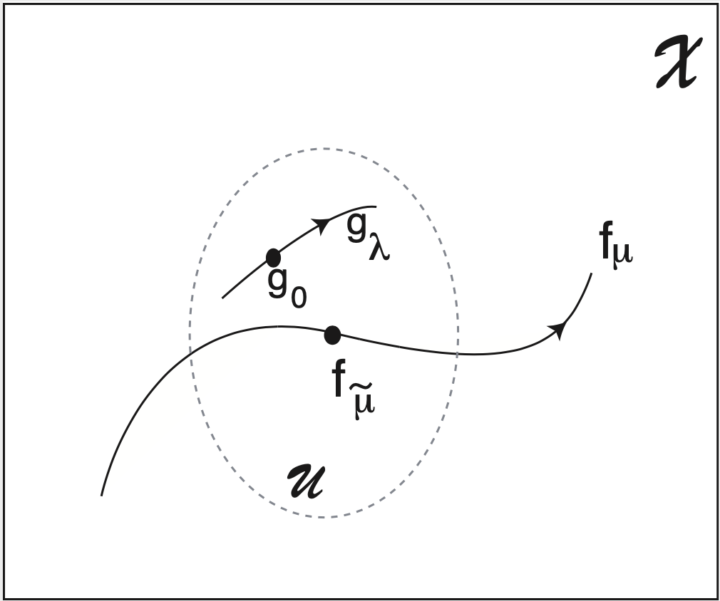
Figure 1. Illustration of the main idea of Theorem A: for all neighbourhood $\mathcal{U}\subset\mathcal{X}$ of $f_{\tilde{\boldsymbol{\mu}}}$, $\tilde{\boldsymbol{\mu}}\in I$, there exists a generic family $\left(g_{\boldsymbol{\lambda}}\right)_{\boldsymbol{\lambda}\in[-1,1]}\in\mathcal{U}$ exhibiting persistently strange attractors.

After studying the dynamics of the differential equation (6), we prove Theorem A by making use of a homoclinic cycle to the interior equilibrium (of Shilnikov type), whose existence is a criterion for observable and persistent chaotic dynamics. The core of the present work goes further: we describe the phenomenological scenario leading to the emergence of a strange attractor.

4. Bifurcation analysis

We proceed to the analysis of the one-parameter family of differential equations (6). We describe the dynamics on the different faces, including the emergence of different equilibria on the edges. Our analysis will be focused on $\boldsymbol{\mu}\in\left[-\frac{2938}{95},10\right]$, where a unique equilibrium exists in $[0,1]^{3}$. This equilibrium will play an important role in the emergence of the strange attractor.

In what follows, we list some assertions that have been analytically found.

4.1. Boundary

We describe the equilibria and bifurcations on the boundary of $[0,1]^{3}$ as function of $\boldsymbol{\mu}$. The equilibria of system (6) do not necessarily belong to the cube. Throughout this article, the equilibria are those that lie on $[0,1]^{3}$ and formal equilibria (as defined in [2, Def. 4.1]) lie outside it.

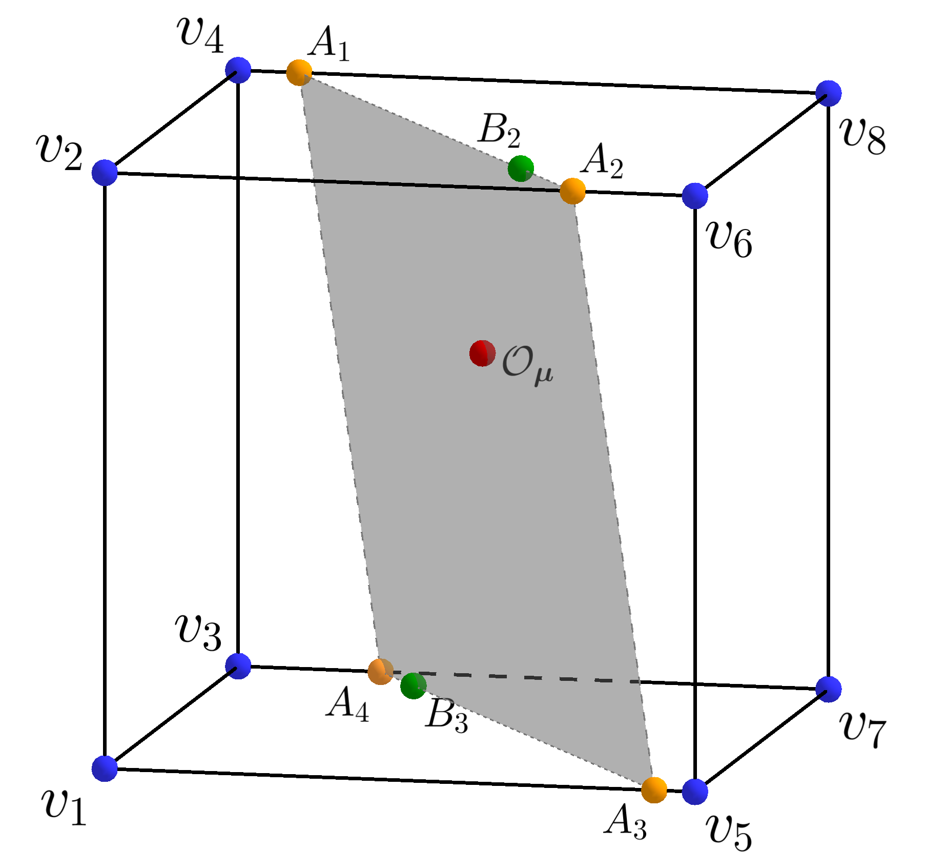
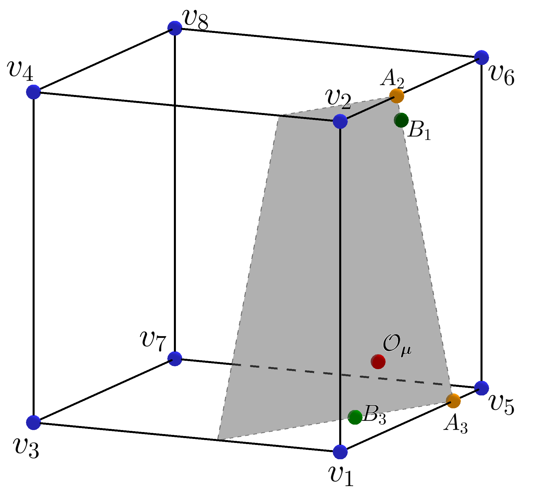
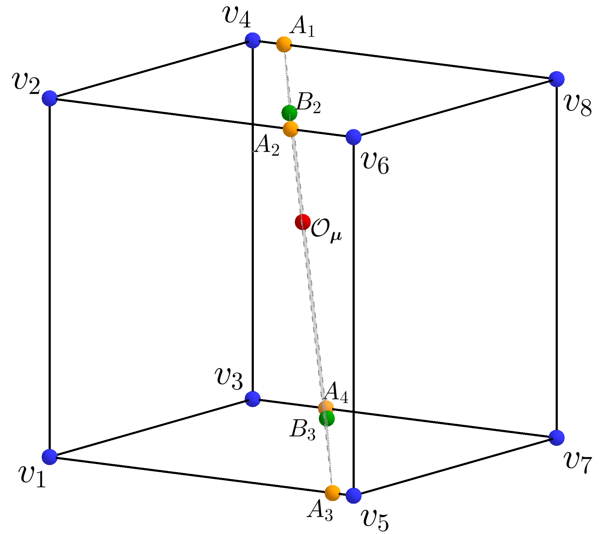
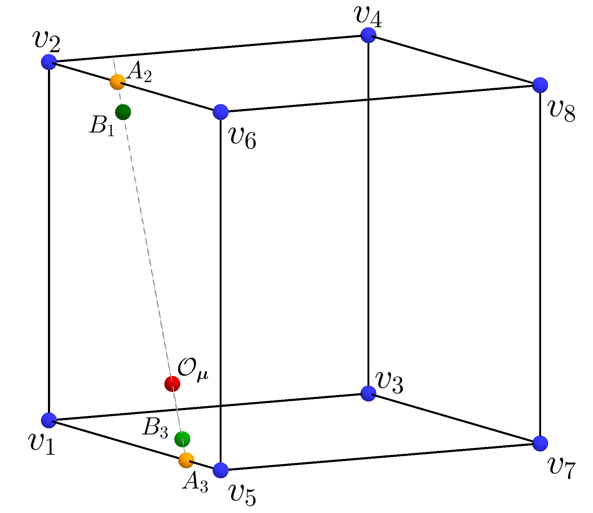
Figure 2. Different perspectives of the phase space and the corresponding equilibria of (6): the eight vertices $v_{1},\dots,v_{8}$ (in blue), four equilibria on edges, $A_{1},A_{2},A_{3},A_{4}$ (in orange), three equilibria on faces, $B_{1},B_{2},B_{3}$ (in green), and the interior equilibrium $\mathcal{O}_{\boldsymbol{\mu}}$ (in red), for $\boldsymbol{\mu}=-15$ (top) and $\boldsymbol{\mu}=4$ (bottom). These equilibria lie on a plane (se the remark after Lemma 4).

From now on, all the figures with numerical plots of the flow of (6) on $[0,1]^{3}$ are in the same position of Figure 2 (up left) where $v_{1}=(0,0,0)$ is the vertex located in the lower left front corner.

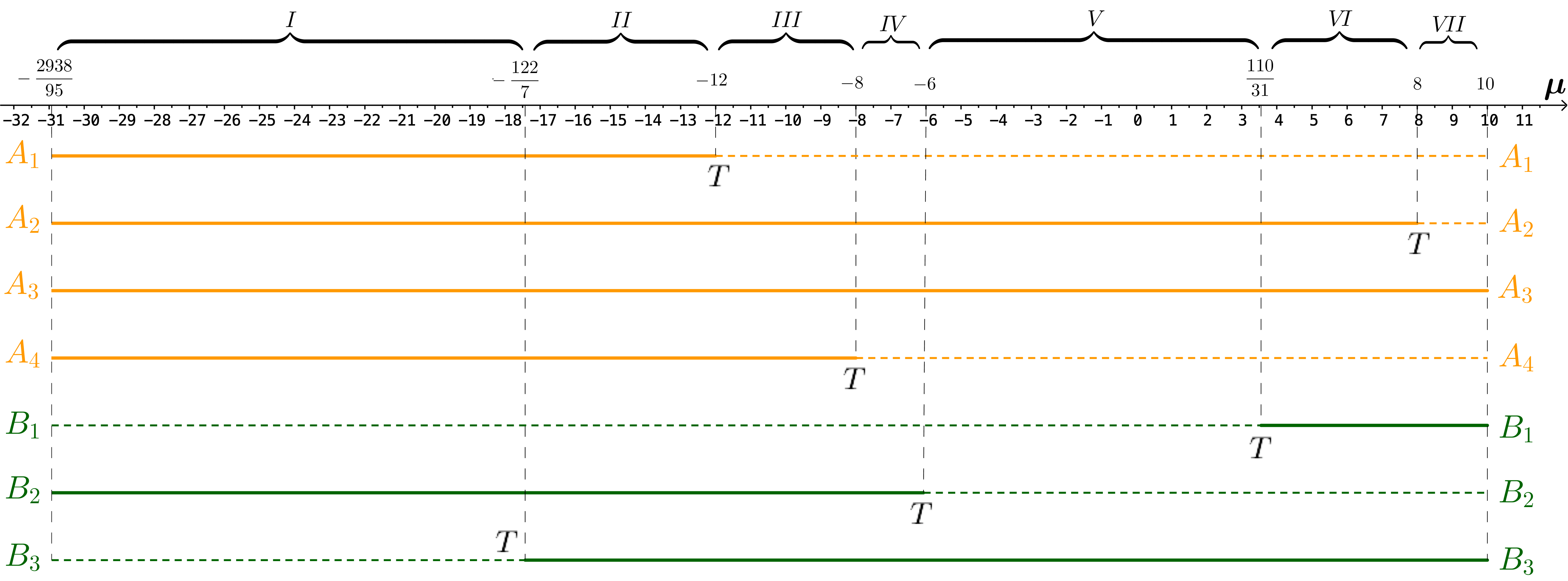
Figure 3. The values of $\boldsymbol{\mu}$ for which the equilibria of system (6) exist on $[0,1]^{3}$ (continuous line) and outside $[0,1]^{3}$ (dashed line) – formal equilibria. The Roman numerals $\textup{I},\dots,\textup{VII}$ represents the cases of Table 2 and the letter $T$ corresponds to the values of $\boldsymbol{\mu}$ for which a transcritical bifurcation occur.

We describe a list of equilibria that appear on the edges and faces of the cube $[0,1]^{3}$, as function of the parameter $\boldsymbol{\mu}$. The cube has six faces defined by, for $i\in\{1,3,5\}$,

$$\sigma_{i} :\qquad x_{i+1}=1$$

$$\sigma_{i+1} :\qquad x_{i+1}=0.$$

In Table 2 we identify the vertices that belong to each face. As suggested in Figure 2, we set the notation $A_{j}$, $j=1,2,3,4$ for equilibria on the edges and $B_{j}$, $j=1,2,3$ for equilibria on the interior of the faces. Formally, the $A$’s and $B$’s equilibria depend on $\boldsymbol{\mu}$ but, once again, we omit their dependence on the parameter.

Lemma 3.

With respect to system (6), for $\boldsymbol{\mu}\in[-\frac{2938}{95},10]$, the following assertions hold:

1. The eight vertices and $A_{3}=\left(\frac{12-\boldsymbol{\mu}}{14-\boldsymbol{\mu}},0,0\right)$ exist for $\boldsymbol{\mu}\in\left[-\frac{2938}{95},10\right]$,

2. $A_{1}=\left(\frac{\boldsymbol{\mu}+12}{\boldsymbol{\mu}-14},1,1\right)\,\textrm{exists in the cube}\quad\Leftrightarrow\quad\boldsymbol{\mu}\in\left[-\frac{2938}{95},-12\right[$,

3. $A_{4}=\left(\frac{8+\boldsymbol{\mu}}{\boldsymbol{\mu}-14},1,0\right)\,\textrm{exists in the cube}\quad\Leftrightarrow\quad\boldsymbol{\mu}\in\left[-\frac{2938}{95},-8\right[$,

4. $A_{2}=\left(\frac{8-\boldsymbol{\mu}}{14-\boldsymbol{\mu}},0,1\right)\,\textrm{exists in the cube}\quad\Leftrightarrow\quad\boldsymbol{\mu}\in\left[-\frac{2938}{95},8\right[$,

5. $B_{1}=\left(\frac{15+\boldsymbol{\mu}}{40+\boldsymbol{\mu}},0,\frac{27(10-\boldsymbol{\mu})}{4(40+\boldsymbol{\mu})}\right)\,\textrm{exists in the cube}\quad\Leftrightarrow\quad\boldsymbol{\mu}\in\left]\frac{110}{31},10\right]$,

6. $B_{2}=\left(\frac{62+\boldsymbol{\mu}}{86+\boldsymbol{\mu}},-\frac{3(6+\boldsymbol{\mu})}{2(86+\boldsymbol{\mu})},1\right)\,\textrm{exists in the cube}\quad\Leftrightarrow\quad\boldsymbol{\mu}\in\left[-\frac{2938}{95},-6\right[$,

7. $B_{3}=\left(\frac{38+\boldsymbol{\mu}}{86+\boldsymbol{\mu}},\frac{5(10-\boldsymbol{\mu})}{2(86+\boldsymbol{\mu})},0\right)\,\textrm{exists in the cube}\quad\Leftrightarrow\quad\boldsymbol{\mu}\in\left]-\frac{122}{7},10\right]$.

The proof of Lemma 3 is elementary by computing zeros of $f_{\boldsymbol{\mu}}$ and taking into account that they should live in $[0,1]^{3}$. The evolution (as function of $\boldsymbol{\mu}$) of the equilibria $A_{1},A_{2},A_{3},A_{4}$ on the edges and $B_{1},B_{2},B_{3}$ on the faces is depicted in the scheme of Figure 3. The eigenvalues and eigendirections are summarised in Tables 3 and 4. Using the sign of the eigenvalues, as well as their evolution, we are able to locate transcritical bifurcations, which are summarised in the following paragraph and pointed out in Figure 3.

We will consider sub-intervals of $[-\frac{2938}{95},10]$ based on the values of $\boldsymbol{\mu}$ for which the bifurcations occur. Namelly:

• at $\boldsymbol{\mu}=-12$ the vertex $v_{4}$ undergoes a transcritical bifurcation (see the zero eigenvalue in Table 5) responsible for the transition of $A_{1}$ from $[0,1]^{3}$ to outside, becoming a formal equilibrium; the analysis of the bifurcation associated to $A_{2}$ and $A_{4}$ is similar at $\boldsymbol{\mu}=8$ and $\boldsymbol{\mu}=-8$, respectively;

• at $\boldsymbol{\mu}=-6$, the equilibrium $A_{2}$ undergoes a transcritical bifurcation and $B_{2}$ evolves from an equilibrium (inside the cube) to a formal one (outside the cube); the reverse happens to $B_{1}$ at $\boldsymbol{\mu}=\frac{110}{31}$;

• at $\boldsymbol{\mu}=-\frac{122}{7}$, the equilibrium $A_{4}$ undergoes a transcritical bifurcation and $B_{3}$ evolves from a formal equilibrium (outside the cube) to an equilibrium (inside the cube);

• at $\boldsymbol{\mu}=b_{2}\approx-21.9$ (see Table 4) and $\boldsymbol{\mu}=-12$, the equilibrium $B_{2}$ undergoes a Belyakov transition; and, at $\boldsymbol{\mu}=b_{3}\approx-14.22$ the $B_{3}$ also undergoes the same bifurcation (see Table 4).

4.2. Interior

In this section, we focus our attention on the interior equilibrium and its relation to others on the boundary.

Lemma 4.

For $\boldsymbol{\mu}\in\,]-\frac{2938}{95},10[$, system (6) has a unique interior equilibrium, whose expression is

$$\mathcal{O}_{\boldsymbol{\mu}}:=\left(\frac{7\boldsymbol{\mu}-1042}{7\boldsymbol{\mu}-2014},\frac{37(\boldsymbol{\mu}-10)}{7\boldsymbol{\mu}-2014},\frac{109(\boldsymbol{\mu}-10)}{2(7\boldsymbol{\mu}-2014)}\right).$$

Proof.

The proof is immediate by computing the non-trivial zeros of the vector field (6):

$$\left\{\begin{array}[]{l}12-\boldsymbol{\mu}+(\boldsymbol{\mu}-14)x-20y-4z=0\\[5.69054pt] -10+20x+4y-4z=0\\[5.69054pt] 27-54x+11y-4z=0\end{array}\right..$$

∎

Taking into account that the equilibria $B_{1}$, $B_{2}$ and $B_{3}$ depend on $\boldsymbol{\mu}$, it is worth to notice that

$$\lim_{\boldsymbol{\mu}\rightarrow-\frac{2938}{95}}\mathcal{O}_{\boldsymbol{\mu}}=\lim_{\boldsymbol{\mu}\rightarrow-\frac{2938}{95}}B_{2}=\left(\frac{123}{218},\frac{74}{109},1\right)$$

and

$$\lim_{\boldsymbol{\mu}\rightarrow 10}\mathcal{O}_{\boldsymbol{\mu}}=\lim_{\boldsymbol{\mu}\to 10}B_{1}=\lim_{\boldsymbol{\mu}\to 10}B_{3}=\left(\frac{1}{2},0,0\right),$$

which means that when $\boldsymbol{\mu}\in\,]-\frac{2938}{95},10]$, the point $O_{\boldsymbol{\mu}}$ travels from the face $\sigma_{5}$ to the edge which connects $v_{1}$ to $v_{5}$, the intersection of the faces $\sigma_{4}$ and $\sigma_{6}$.

Remark.

The points $A_{1}$, $A_{2}$, $A_{3}$, $A_{4}$, $B_{1}$, $B_{2}$, $B_{3}$ and $\mathcal{O}_{\boldsymbol{\mu}}$ belong to the plane defined by $(14-\boldsymbol{\mu})x+20y+{4}z={12-\boldsymbol{\mu}}.$ This follows immediately from the first equation of system (6). This plane is not flow-invariant.

Lemma 5.

With respect to $Df_{\boldsymbol{\mu}}\left(\mathcal{O}_{\boldsymbol{\mu}}\right)$, there exist $\mu_{1},\mu_{2},\mu_{4}\in[-\frac{2938}{95},10]$ such that $\mu_{1}<\mu_{2}<\mu_{4}$ and:

1. for $\boldsymbol{\mu}=\mu_{1}$, the equilibrium $\mathcal{O}_{\boldsymbol{\mu}}$ undergoes a Belyakov transition;

2. for $\boldsymbol{\mu}=\mu_{2}$ and $\boldsymbol{\mu}=\mu_{4}$ the equilibrium $\mathcal{O}_{\boldsymbol{\mu}}$ undergoes a supercritical Hopf bifurcation.

Proof.

The characteristic polynomial of $Df_{\boldsymbol{\mu}}\left(\mathcal{O}_{\boldsymbol{\mu}}\right)$ has three roots, which depend on $\boldsymbol{\mu}$. Although these three functions have an intractable analytical expression, it is possible to show the existence of $\mu_{1},\mu_{2},\mu_{4}\in[-\frac{2938}{95},10]$ such that $\mu_{1}<\mu_{2}<\mu_{4}$ and the following assertions hold (cf. Figures 4 and 5):

1. for $\boldsymbol{\mu}\in[-\frac{2938}{95},\mu_{1}]$, the three eigenvalues are real and negative;

2. for $\boldsymbol{\mu}\in\,\,]\mu_{1},\mu_{2}[\,\cup\,]\mu_{4},10]$, there are two complex conjugate eigenvalues and one real, all of them with negative real part;

3. for $\boldsymbol{\mu}\in\,\,]\mu_{2},{\mu}_{4}[$, there are two complex conjugate eigenvalues with positive real part and one real negative.

As suggested by Figure 5, the complex (non-real) eigenvalues cross the imaginary axis with strictly positive speed as $\boldsymbol{\mu}$ passes through ${\mu}_{2}$ and ${\mu}_{4}$, confirming that:

$$\frac{Re\left(Df_{\boldsymbol{\mu}}\left(\mathcal{O}_{\boldsymbol{\mu}}\right)\right)}{d\,\boldsymbol{\mu}}|_{\boldsymbol{\mu}={\mu}_{2}}\neq 0\neq\frac{Re\left(Df_{\boldsymbol{\mu}}\left(\mathcal{O}_{\boldsymbol{\mu}}\right)\right)}{d\,\boldsymbol{\mu}}|_{\boldsymbol{\mu}={\mu}_{4}}.$$

This means that at $\boldsymbol{\mu}=\mu_{2}$ and $\boldsymbol{\mu}=\mu_{4}$, the equilibrium $\mathcal{O}_{\boldsymbol{\mu}}$ undergoes a supercritical Hopf bifurcation. When $\boldsymbol{\mu}=\mu_{2}$, it gives rise to a non-trivial attracting periodic solution, say $\mathcal{C}_{\boldsymbol{\mu}}$, which collapses again into $\mathcal{O}_{\boldsymbol{\mu}}$ for $\boldsymbol{\mu}=\mu_{4}$.

∎

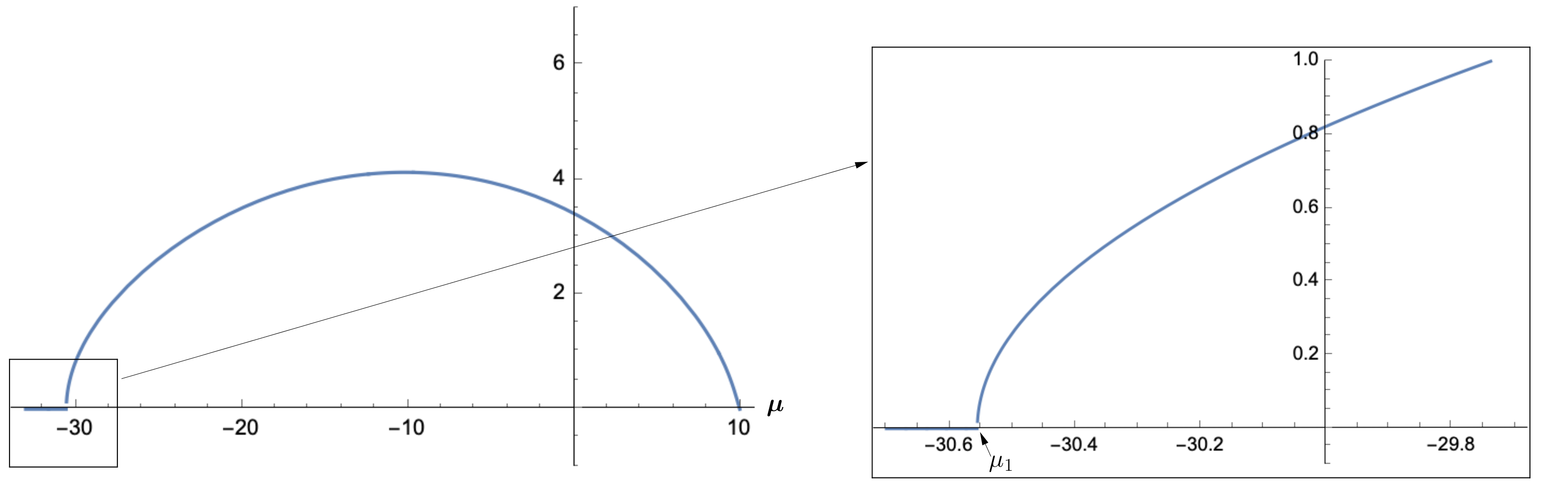
Figure 4. Belyakov transition: graph of the imaginary part of the complex eigenvalues of $Df_{\boldsymbol{\mu}}\left(\mathcal{O}_{\boldsymbol{\mu}}\right)$ for $\boldsymbol{\mu}\in\left[-\frac{2938}{95},10\right]$ (left) and its zoom around $\mu_{1}$, $\boldsymbol{\mu}\in\left[-30.7,-29.7\right]$ (right), for system (6).

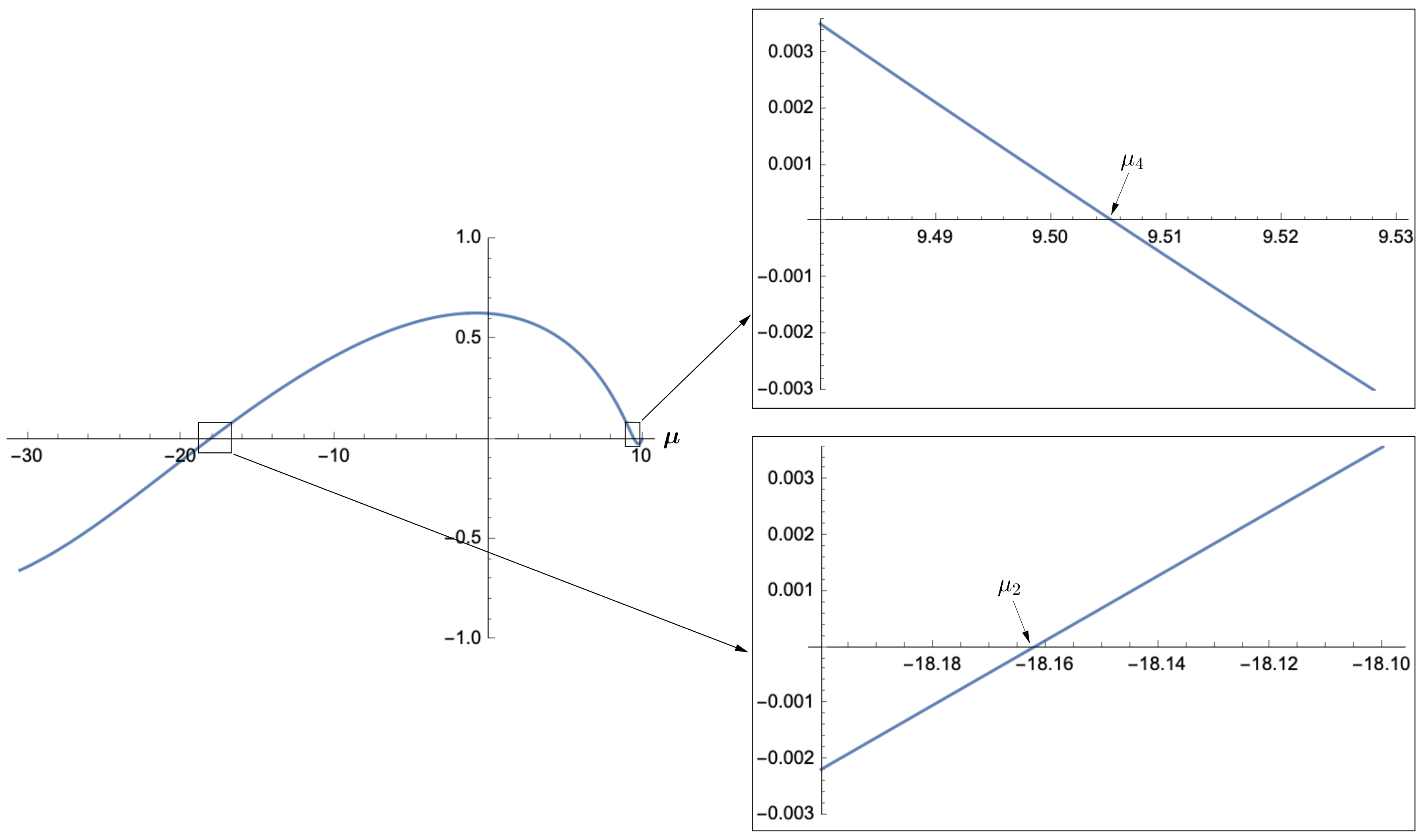
Figure 5. Hopf bifurcation: graph of the real part of the eigenvalues of $Df_{\boldsymbol{\mu}}\left(\mathcal{O}_{\boldsymbol{\mu}}\right)$ for $\boldsymbol{\mu}\in\left[-\frac{2938}{95},10\right]$ (left) and its zoom around $\mu_{4}$, $\boldsymbol{\mu}\in\left[9.48,9.53\right]$ (right up) and around $\mu_{2}$, $\boldsymbol{\mu}\in\left[-18.2,-18.1\right]$ (right down), for system (6).

From now on, we set:

$$\mu_{1} \mapsto \boldsymbol{\mu}_{\textrm{Belyakov}}\approx-30.5550;$$

$$\mu_{2} \mapsto \boldsymbol{\mu}^{1}_{\textrm{Hopf}}\approx-18.1623;$$

$$\mu_{4} \mapsto \boldsymbol{\mu}^{2}_{\textrm{Hopf}}\approx 9.5055.$$

For $\boldsymbol{\mu}\in[-\frac{2938}{95},\mu_{2}]$, the equilibrium $\mathcal{O}_{\boldsymbol{\mu}}$ is globally attracting as depicted in Figure 6. In the context of Game Theory, it is called a global attracting mixed Nash equilibrium, in the sense that it is associated to non-pure strategies.

Figure 6. Global attractiveness of $\mathcal{O}_{\boldsymbol{\mu}}$ (cf. Proposition 6 $(1)$): plot of two orbits (in blue) with initial condition near $v_{1}$ (left), initial condition near $v_{6}$ (right), the interior equilibrium (in red) and the boundary equilibria of system (6) for $\boldsymbol{\mu}=-20$ and $t\in[0,50]$.

5. Numerical Analysis

Using $\textit{Mathematica Wolfram}^{\circledR}$, we present checkable numerical evidences about the vector field $f_{\boldsymbol{\mu}}$, for $\boldsymbol{\mu}\in[-\frac{2938}{95},10]$, that will constitute the foundations for the persistence of strange attractors. At the end of this section we discuss the validity of these numerical results.

5.1. Lyapunov exponents

Using the method in Sandri  [22], in Figure 7 we computed numerically the LE of system (6) for an initial condition of the form:

$$(x_{0},y_{0},z_{0})=\mathcal{O}_{\boldsymbol{\mu}}+\left\{\begin{array}[]{ll}(\varepsilon,0,-\varepsilon),&\textrm{if }\boldsymbol{\mu}\in[-\frac{2938}{95},-30[\\[5.69054pt] (0,0,\varepsilon),&\textrm{if }\boldsymbol{\mu}\in[-30,9]\\[5.69054pt] (\varepsilon,\varepsilon,0),&\textrm{if }\boldsymbol{\mu}\in\,\,]9,10]\end{array}\right.,$$

with $\varepsilon=0.001$, thus ensuring that $(x_{0},y_{0},z_{0})\in{\rm int}\left([0,1]^{3}\right)\backslash W^{s}(\mathcal{O}_{\boldsymbol{\mu}})$. As suggested in [26], since $(x_{0},y_{0},z_{0})\notin W^{s}(\mathcal{O}_{\boldsymbol{\mu}})$, its trajectory is strongly governed by the invariant manifold $W^{u}(\mathcal{O}_{\boldsymbol{\mu}})$, which plays an essential role in the construction of the Hénon-type strange attractor of Theorem A. From a close analysis of Figure 7, we deduce that:

1. for $\boldsymbol{\mu}<\boldsymbol{\mu}^{1}_{\textrm{Hopf}}$ and $\boldsymbol{\mu}>\boldsymbol{\mu}^{2}_{\textrm{Hopf}}$, the three LE are negative;

2. there exists $\mu_{3}\in\,\,]\boldsymbol{\mu}^{1}_{\textrm{Hopf}},\boldsymbol{\mu}^{2}_{\textrm{Hopf}}[$ such that:

   1. for $\boldsymbol{\mu}\in\,]\boldsymbol{\mu}^{1}_{\textrm{Hopf}},\mu_{3}[$, there are two negative LE and one zero;

   2. there are non-trivial subintervals of $]\mu_{3},\boldsymbol{\mu}^{2}_{\textrm{Hopf}}[$ where there is one positive LE.

From this analysis, according to [22, 27], we infer that the attracting set of system (6), when restricted to the cube’s interior, contains:

1. a single equilibrium, for $\boldsymbol{\mu}<\boldsymbol{\mu}^{1}_{\textrm{Hopf}}$ (Figure 6) and $\boldsymbol{\mu}>\boldsymbol{\mu}^{2}_{\textrm{Hopf}}$;

2. a non-trivial periodic solution, for $\boldsymbol{\mu}\in\,]\boldsymbol{\mu}^{1}_{\textrm{Hopf}},\mu_{3}[$ (Figure 11);

3. a strange attractor for some intervals of $]\mu_{3},\boldsymbol{\mu}^{2}_{\textrm{Hopf}}[$ (it follows from $(2)\textrm{(b)}$ and the classification of [27]).

Since $\mu_{3}$ is the threshold above which we find numerically strange attractors (Figure 7), we set

$$\mu_{3} \mapsto\boldsymbol{\mu}_{\textrm{SA}}\approx{1.4645}.$$

As referred in Section 3, a LE is a limit over the variable $t$ and numerical computations require its truncation. Since for $\boldsymbol{\mu}>\boldsymbol{\mu}^{1}_{\textrm{Hopf}}$ there is at least one LE oscillating around the zero value, we decided to consider positive LE those greater than $5\times 10^{-3}$. This will allow to discard uncertain positive Lyapunov exponents due to numerical precision issues. Lower precision would complicate the simulations bringing no better results.

Figure 7. Sign of the Lyapunov exponents: linear interpolation of the largest non-zero Lyapunov exponents of system (6) with initial condition near the interior equilibrium ($\notin W^{s}(\mathcal{O}_{\boldsymbol{\mu}})$). $(-,-,-)$: all LE are negative. $(-,-,0)$: one LE is zero and the other are negative. $(-,0,+)$: one LE is negative, one is positive and the other is zero.

5.2. Numerical facts

In this subsection, based on numerics, we list some evidences (hereafter called by Facts) about system (6). They are essential to characterise the route to chaos in Section 6 and may be numerically checked.

Fact 1.

In the parameter interval $\boldsymbol{\mu}\in\,\,]-\frac{2938}{95},10[$:

1. for $\boldsymbol{\mu}<-8$ there exist two heteroclinic connections from $v_{3}$ and $v_{6}$ to $\mathcal{O}_{\boldsymbol{\mu}}$ (Figure 8 (left));

2. for $\boldsymbol{\mu}\in\,]-8,\boldsymbol{\mu}_{\textrm{SA}}[\,\cup\,]\boldsymbol{\mu}^{2}_{\textrm{Hopf}},10[$, there are two heteroclinic connections from the source $v_{6}$ to $\mathcal{O}_{\boldsymbol{\mu}}$, along the two branches of $W^{s}(\mathcal{O}_{\boldsymbol{\mu}})$ (Figure 8 (right));

3. for $\boldsymbol{\mu}\in\,]\boldsymbol{\mu}_{\textrm{SA}},\boldsymbol{\mu}^{2}_{\textrm{Hopf}}[$, one branch of $W^{s}(\mathcal{O}_{\boldsymbol{\mu}})$ winds around the non-wandering set associated to $W^{u}(\mathcal{O}_{\boldsymbol{\mu}})$.

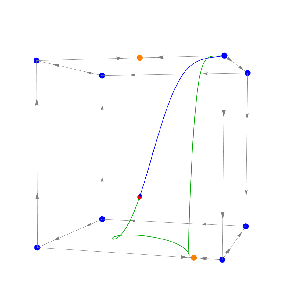
Figure 8. Heteroclinic connections (cf. Fact 1): representation of the connections from the sources $v_{3}$ (in green) and $v_{6}$ (in blue) to $\mathcal{O}_{\boldsymbol{\mu}}$, for system (6) with $\boldsymbol{\mu}=-20$ (left) and $\boldsymbol{\mu}=0$ (right). At $\boldsymbol{\mu}=-8$ the equilibrium $A_{4}$ collapses with $v_{3}$, which makes the lower branch of $W^{u}(\mathcal{O}_{\boldsymbol{\mu}})$ to connect $v_{6}$, a phenomenon that persists for $\boldsymbol{\mu}>-8$.

Fact 2.

For $\boldsymbol{\mu}\in\left]\boldsymbol{\mu}^{1}_{\textrm{Hopf}},\boldsymbol{\mu}^{2}_{\textrm{Hopf}}\right[$ the eigenvalues of $Df_{\boldsymbol{\mu}}\left(\mathcal{O}_{\boldsymbol{\mu}}\right)$ are of the form

$$\lambda_{\textrm{u}}(\boldsymbol{\mu})\pm i\omega(\boldsymbol{\mu})\quad\textrm{and}\quad-\lambda_{\textrm{s}}(\boldsymbol{\mu}),$$

where

$$\lambda_{\textrm{u}}(\boldsymbol{\mu}),\omega(\boldsymbol{\mu}),\lambda_{\textrm{s}}(\boldsymbol{\mu})>0,\quad 2\lambda_{\textrm{u}}(\boldsymbol{\mu})<\lambda_{\textrm{s}}(\boldsymbol{\mu})\quad\textrm{ and }\quad\frac{d}{d\boldsymbol{\mu}}\left(\frac{\lambda_{u}(\boldsymbol{\mu})}{\lambda_{s}(\boldsymbol{\mu})}\right)\neq 0.$$

Fact 3.

There are non-trivial subintervals of $\left]\mu_{3},\boldsymbol{\mu}^{2}_{\textrm{Hopf}}\right[$ where $f_{\boldsymbol{\mu}}$ has one positive LE (Figure 7).

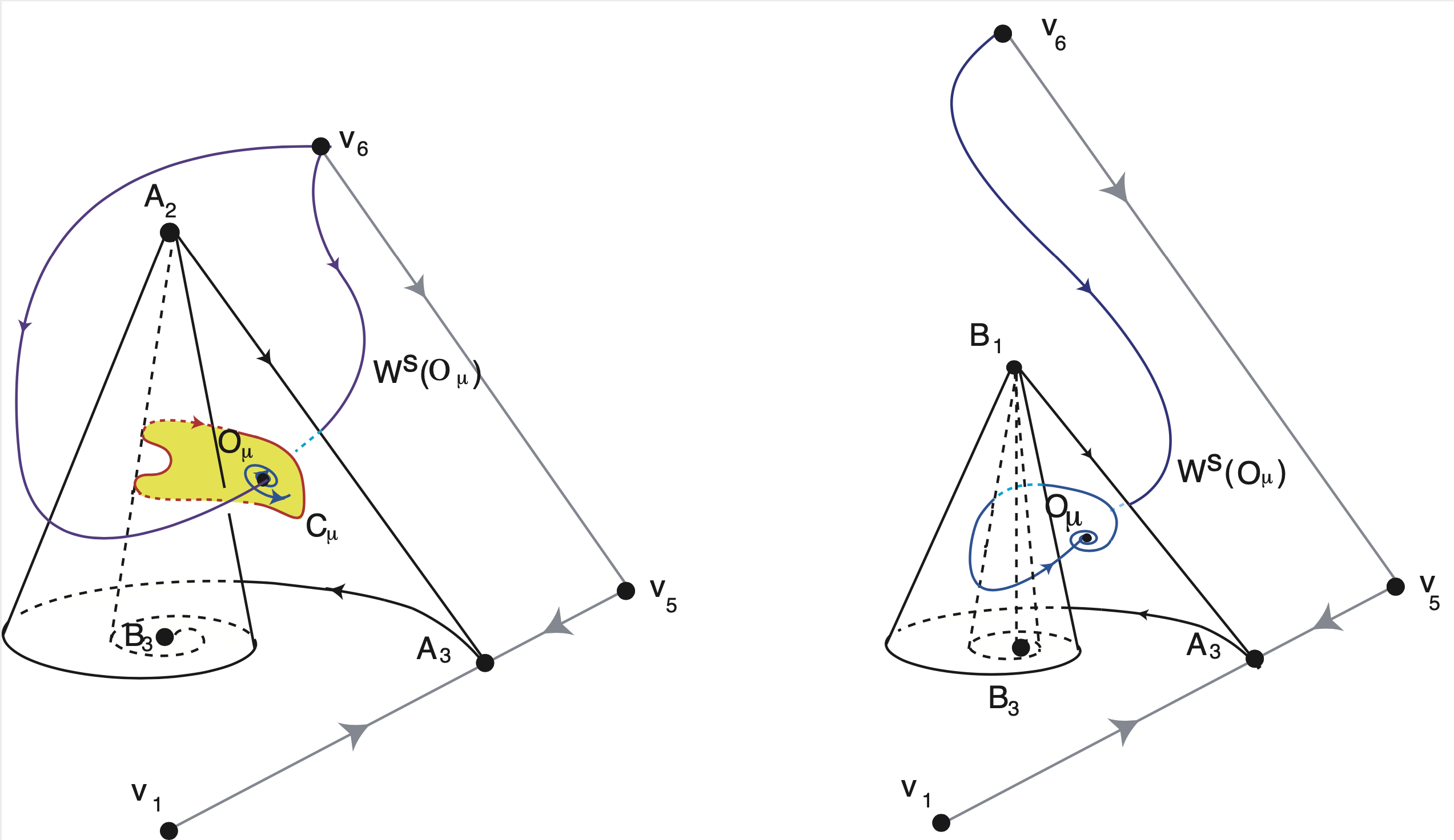
Figure 9. The attracting whirlpool (see Proposition 11) : illustration of Fact 2 (left) and Fact 3 (right). For the values of $\boldsymbol{\mu}$ for which the greatest LE of $f_{\boldsymbol{\mu}}$ is positive, there exists a vector field close to $f_{\boldsymbol{\mu}}$ whose flow exhibits a homoclinic orbit to $\mathcal{O}_{\boldsymbol{\mu}}$. A description of the attracting whirlpool is given in detail in Subsection 8.1.

Fact 4.

For $\boldsymbol{\mu}\in\,\,]\frac{110}{31},8[$ , we have $[v_{5}\rightarrow v_{6}]\subset\overline{W^{s}(B_{1})}$.

Let $I\subset\left]\boldsymbol{\mu}_{\textrm{SA}},\boldsymbol{\mu}^{2}_{\textrm{Hopf}}\right[$ be a non-degenerate interval of $\boldsymbol{\mu}$-values for which the greatest LE of $f_{\boldsymbol{\mu}}$ is positive.

Fact 5.

For $\boldsymbol{\mu}\in I\subset\left]\boldsymbol{\mu}_{\textrm{SA}},\boldsymbol{\mu}^{2}_{\textrm{Hopf}}\right[$, there exists a $C^{2}$–vector field $g\in\mathcal{X}$ arbitrarily close to $f_{\boldsymbol{\mu}}$ (in the $C^{2}$-topology), whose flow exhibits a homoclinic orbit to the hyperbolic continuation of $\mathcal{O}_{\boldsymbol{\mu}}$ (Figure 10).

5.3. Digestive remark

Facts 1–5 have been numerically checked both in $\textit{Mathematica Wolfram}^{\circledR}$ and $\textrm{MATLAB}^{\circledR}$.

We give a heuristic justification why Fact 5 may be considered a consequence of Fact 3. The existence of a positive Lyapunov exponent for $f_{\boldsymbol{\mu}}$ (Fact 3) implies the existence of an invariant subset of $\mathbb{R}^{3}$ with positive topological entropy (Corollary 4.3 of [29]), leading to the existence of a transverse homoclinic point and horseshoes. Besides the equilibrium $\mathcal{O}_{\boldsymbol{\mu}}$ and the attracting periodic solution $\mathcal{C}_{\boldsymbol{\mu}}$, the flow of (6) does not have more nontrivial compact invariant sets in ${\rm int}([0,1]^{3})$ for $\mu<\boldsymbol{\mu}_{SA}$. Therefore, the only way to realize these horseshoes is through a homoclinic cycle to the hyperbolic continuation of $\mathcal{O}_{\boldsymbol{\mu}}$ for $\mu>\boldsymbol{\mu}_{SA}$ (Fact 5). This agrees with numerics.

Figure 10. The plot of the stable (in red) and the unstable (in blue) manifolds of $\mathcal{O}_{\boldsymbol{\mu}}$, for system (6) with $\boldsymbol{\mu}=3.6$.

6. Route to strange attractors

Using the same type of arguments of [30, 31], we explain the global dynamics of system (6) in ${\rm int}\left([0,1]^{3}\right)$ according to the local bifurcations studied in Section 4. Based on the transcritical bifurcations of the equilibria on the boundary and the bifurcations of $\mathcal{O}_{\boldsymbol{\mu}}$, we distinguish the seven cases described in Table 2 and we make use of the Facts stated in Section 5, to prove the existence of chaos. We also denote by $\mathcal{F}$ the union of all faces, i.e. $\mathcal{F}=\{\sigma_{1},\dots,\sigma_{6}\}$.

Case		Interval of $\boldsymbol{\mu}$
I	$\textup{I}.1$	$]-\frac{2938}{95},\boldsymbol{\mu}_{\textrm{Belyakov}}[$
	$\textup{I}.2$	$]\boldsymbol{\mu}_{\textrm{Belyakov}},\boldsymbol{\mu}^{1}_{\textrm{Hopf}}[$
	$\textup{I}.3$	$]\boldsymbol{\mu}^{1}_{\textrm{Hopf}},-\frac{122}{7}[$
II		$]-\frac{122}{7},-12[$
III		$]-12,-8[$

Case		Interval of $\boldsymbol{\mu}$
IV		$]-8,-6[$
V		$]-6,\frac{110}{31}[$
VI		$]\frac{110}{31},8[$
VII	$\textup{VII}.1$	$]8,\boldsymbol{\mu}^{2}_{\textrm{Hopf}}[$
	$\textup{VII}.2$	$]\boldsymbol{\mu}^{2}_{\textrm{Hopf}},10[$

Table 2. The sub-intervals (that we designate as Cases) of $]-\frac{2938}{95},10[$ based on the values of $\boldsymbol{\mu}$ for which the bifurcations occur on the boundary (Cases $\textup{I},\dots,\textup{VII}$) and on the interior equilibrium (Cases $\textup{I}.1,\textup{I}.2,\textup{I}.3$ and $\textup{VII}.1,\textup{VII}.2$).

We illustrate our results with numerical simulations for values of the parameter in each case of Table 2. In Appendices B and  C, all figures are collected to allow a global understanding of the route to chaos. We divide the pictures in two cases: dynamics on the boundary (Table 6) and on the cube’s interior (Table 7).

Proposition 6.

In Case I, there exists an invariant and attracting two-dimensional set $\Sigma_{\boldsymbol{\mu}}$ containing the points $A_{1},A_{2},A_{3},A_{4},B_{2}$ and $\mathcal{O}_{\boldsymbol{\mu}}$, and the heteroclinic connections $[A_{2}\to A_{3}]$, $[A_{3}\to A_{4}]$, $[A_{4}\to A_{1}]$, $[A_{1}\to B_{2}]$, and $[A_{2}\to B_{2}]$. Moreover,

1. In Cases $\textup{I}.1$ and $\textup{I}.2$, if $p\in\Sigma_{\boldsymbol{\mu}}\backslash\mathcal{F}$, then its $\omega$-limit is $\mathcal{O}_{\boldsymbol{\mu}}$.

2. In Case $\textup{I}.3$, if $p\in\Sigma_{\boldsymbol{\mu}}\backslash\left(\mathcal{F}\cup W^{s}(\mathcal{O}_{\boldsymbol{\mu}})\right)$, then its $\omega$-limit is $\mathcal{C}_{\boldsymbol{\mu}}$ ().

In the three Cases, ${\rm int}\left([0,1]^{3}\right)$ is divided by $\Sigma_{\boldsymbol{\mu}}$ in two connected components.

Proof.

By Lemma 2, we know that the faces are invariant. In Cases $\textup{I}.1$ and $\textup{I}.2$, besides the attracting interior equilibrium, there are no more invariant compact sets in ${\rm int}\left([0,1]^{3}\right)$. Therefore, analysing the direction of the flow, the $\omega$-limit of all points in the cube’s interior is the two-dimensional set bounded by the heteroclinic connections $[A_{2}\to A_{3}]$, $[A_{3}\to A_{4}]$, $[A_{4}\to A_{1}]$, $[A_{1}\to B_{2}]$, and $[A_{2}\to B_{2}]$ as depicted in Figure 12 (left). This defines a two-dimensional set $\Sigma_{\boldsymbol{\mu}}$ containing $\mathcal{O}_{\boldsymbol{\mu}}$ which is attracting and invariant (see Figure 6).

In Case $\textup{I}.3$, besides the interior equilibrium $\mathcal{O}_{\boldsymbol{\mu}}$, system (6) exhibits an attracting periodic solution, $\mathcal{C}_{\boldsymbol{\mu}}$, lying on the attracting two-dimensional set $\Sigma_{\boldsymbol{\mu}}$ (observe that this plane is attracting) (see Figure 11 (left)), which emerge from a transcritical Hopf bifurcation by Lemma 5. This two-dimensional set contains $\overline{W^{s}(\mathcal{C}_{\boldsymbol{\mu}})}$. In all cases, since the boundary of $\Sigma_{\boldsymbol{\mu}}$ belongs to the opposite faces $\sigma_{3},\sigma_{4}$ and $\sigma_{5},\sigma_{6}$ of the phase space, it divides its interior in two connected components.

∎

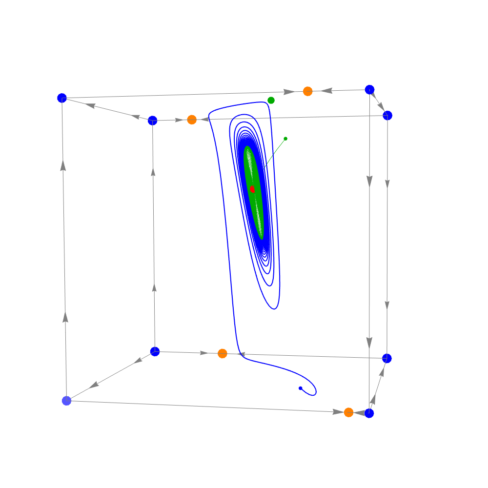
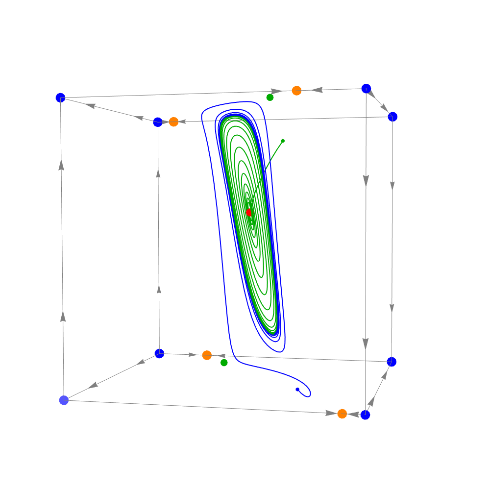
Figure 11. The limit cycle in Cases I and II: plot of two orbits (one in blue and one in green), the interior equilibrium, and all the boundary equilibria of system (6), for $\boldsymbol{\mu}=-17.5$ (left) and $\boldsymbol{\mu}=-14$ (right) with $t\in[0,100]$.

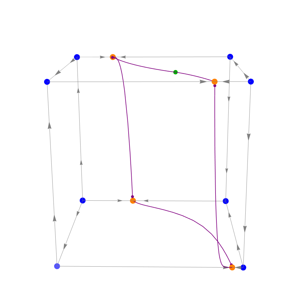
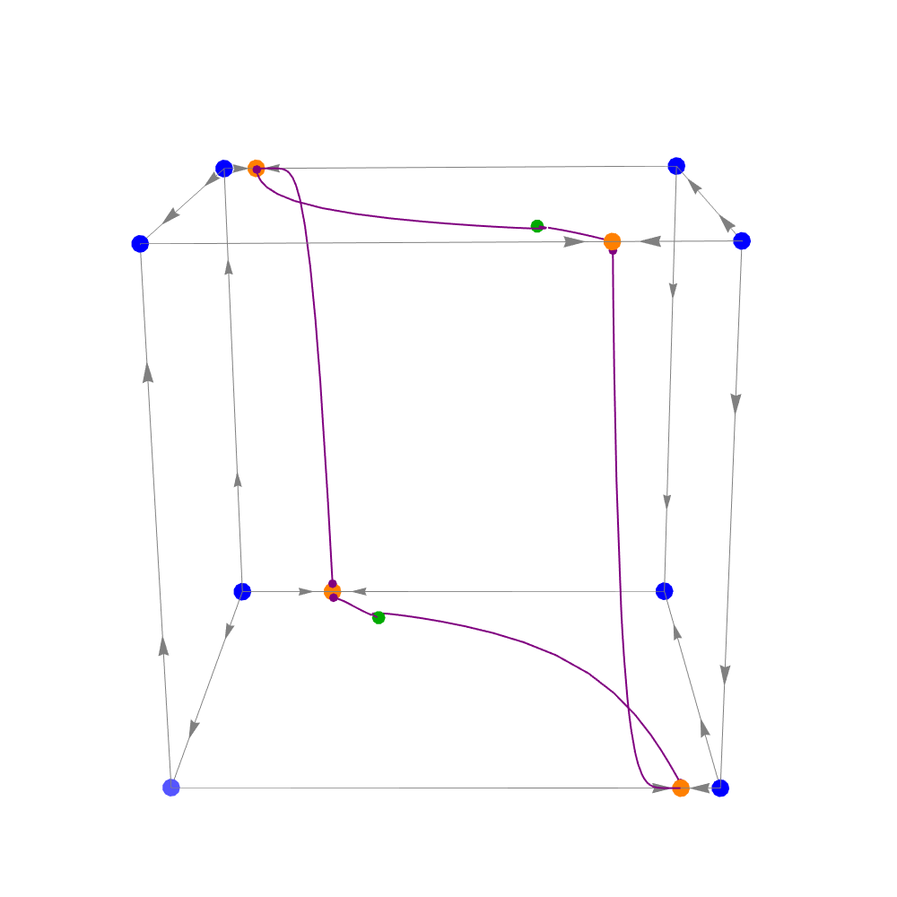
Figure 12. Boundary of $\Sigma_{\boldsymbol{\mu}}$ in Cases I and II: illustration of the dynamics on the boundary in Cases I (left, $\boldsymbol{\mu}=-20$) and II (right, $\boldsymbol{\mu}=-14$).

Proposition 7.

In Case II, there exists an invariant and attracting $2$-dimensional set $\Sigma_{\boldsymbol{\mu}}$ containing the points $A_{1},A_{2},A_{3},A_{4},B_{2},B_{3}$, $\mathcal{O}_{\boldsymbol{\mu}}$, and $\mathcal{C}_{\boldsymbol{\mu}}$. If $p\in\Sigma_{\boldsymbol{\mu}}\backslash\left(\mathcal{F}\cup\{\mathcal{O}_{\boldsymbol{\mu}}\}\right)$, then its $\omega$-limit is $\mathcal{C}_{\boldsymbol{\mu}}$. The set ${\rm int}\left([0,1]^{3}\right)$ is divided by $\Sigma_{\boldsymbol{\mu}}$ in two connected components.

Proof.

The global dynamics in Case II is the same as in Case $\textup{I}.3$, with exception that $A_{4}$ has undergone a transcritical bifurcation from where the saddle $B_{3}$ has evolved from a formal equilibrium to an equilibrium in the cube $[0,1]^{3}$ (see Figure 12 (right)). Using Table 4, we know that $W^{\textrm{u}}(B_{3})$ points out to the interior of the cube. Thus the periodic solution $\mathcal{C}_{\boldsymbol{\mu}}$ is still the $\omega$-limit set of all points in ${\rm int}\left([0,1]^{3}\right)\backslash\left(\{\mathcal{O}_{\boldsymbol{\mu}}\}\cup W^{s}(\mathcal{O}_{\boldsymbol{\mu}})\right)$ (see Figure 11 (right)). Notice also that the ${\rm int}\left([0,1]^{3}\right)$ is still divided by $\Sigma_{\boldsymbol{\mu}}$ in two connected components.

∎

Remark.

The difference between Cases I and II is that $B_{3}$ appears as an equilibrium on the cube in the second scenario. However, the “interior dynamics” does not change qualitatively.

Proposition 8.

In Case III, there exists an invariant and attracting two-dimensional set $\Sigma_{\boldsymbol{\mu}}$ containing the points $v_{2},v_{4},A_{2},A_{3},A_{4},B_{2},B_{3}$, $\mathcal{O}_{\boldsymbol{\mu}}$ and $\mathcal{C}_{\boldsymbol{\mu}}$. The set ${\rm int}\left([0,1]^{3}\right)$ is divided by $\Sigma_{\boldsymbol{\mu}}$ in two connected components.

Proof.

The $\omega$-limit of all points in ${\rm int}\left(\sigma_{5}\right)$ and ${\rm int}\left(\sigma_{6}\right)$ is $B_{2}$ and $B_{3}$, respectively (see Figure 14 (left)). The structure of the two-dimensional set $\Sigma_{\boldsymbol{\mu}}$ on the face $\sigma_{5}$ comes from Proposition 7 and the fact that $A_{1}$ collapses with the vertex $v_{4}$ through a transcritical bifurcation (see Table 3). Notice also that, by continuity from Case II, the ${\rm int}\left([0,1]^{3}\right)$ is still divided by $\Sigma_{\boldsymbol{\mu}}$ in two connected components (see Figure 13 (left)).

∎

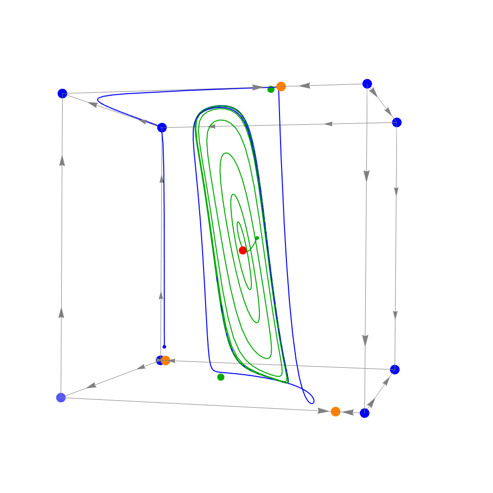
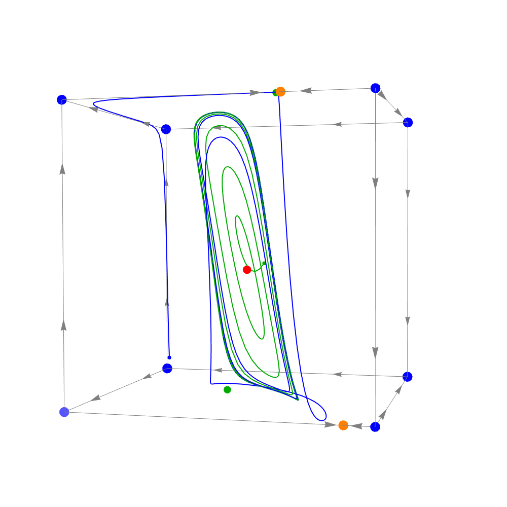
Figure 13. The boundary of $\Sigma_{\boldsymbol{\mu}}$ and the limit cycle in Cases III and IV: plot of two orbits (one in blue and one in green), the interior equilibrium, and all the boundary equilibria of system (6), for $\boldsymbol{\mu}=-8.5$ (left) and $\boldsymbol{\mu}=-7$ (right) with $t\in[0,100]$.

Proposition 9.

In Case IV, there exists an invariant and attracting two-dimensional set $\Sigma_{\boldsymbol{\mu}}$ containing the points $v_{2},v_{3},v_{4},A_{2},A_{3},B_{2},B_{3},\mathcal{O}_{\boldsymbol{\mu}}$, and $\mathcal{C}_{\boldsymbol{\mu}}$. The set ${\rm int}\left([0,1]^{3}\right)$ is divided by $\Sigma_{\boldsymbol{\mu}}$ in two connected components.

Proof.

From Case III to Case IV, the equilibrium $A_{4}$ disappears through a transcritical bifurcation (Table 3). Since the $\omega$-limit of all points in ${\rm int}\left(\sigma_{5}\right)$ and ${\rm int}\left(\sigma_{6}\right)$ is $B_{2}$ and $B_{3}$, respectively (see Figure 14 (right)), the two-dimensional set $\Sigma_{\boldsymbol{\mu}}$ of Case III gives rise to a two-dimensional set containing $\mathcal{C}_{\boldsymbol{\mu}}$ and $\mathcal{O}_{\boldsymbol{\mu}}$ (see Figure 13 (right)). Notice that ${\rm int}\left([0,1]^{3}\right)$ is divided by $\Sigma_{\boldsymbol{\mu}}$ in two connected components, and the latter set is still attracting.

∎

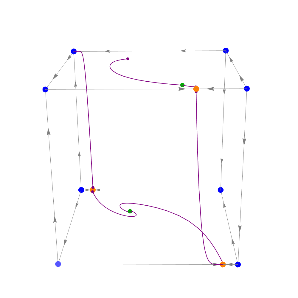
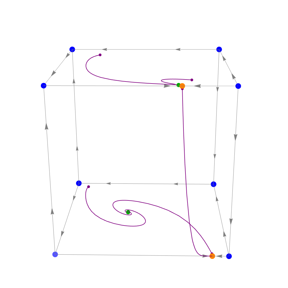
Figure 14. The boundary of $\Sigma_{\boldsymbol{\mu}}$ in Cases III and IV: illustration of the dynamics on the boundary in Cases III (left, $\boldsymbol{\mu}=-10$) and IV (right, $\boldsymbol{\mu}=-7$).

By Fact 1, for $\boldsymbol{\mu}\in\,]\boldsymbol{\mu}^{1}_{\textrm{Hopf}},-8[$ (Cases I–III), the two branches of $W^{s}(\mathcal{O}_{\boldsymbol{\mu}})$ are connected with the sources $v_{3}$ and $v_{6}$. From Case IV on, the equilibrium $v_{3}$ changes stability and the two branches of $W^{s}(\mathcal{O}_{\boldsymbol{\mu}})$ are connected with $v_{6}$ in different eigenspaces. Dramatic changes occur in Case V.

Proposition 10.

In Case V, there exists an invariant and attracting two-dimensional set $\Sigma_{\boldsymbol{\mu}}$ containing the points $A_{2},A_{3},B_{3}$, $\mathcal{O}_{\boldsymbol{\mu}}$, and $\mathcal{C}_{\boldsymbol{\mu}}$. This manifold is $\overline{W^{s}(\mathcal{C}_{\boldsymbol{\mu}})}$ and the set $\Sigma_{\boldsymbol{\mu}}$ does not divide ${\rm int}\left([0,1]^{3}\right)$ in two connected components. Moreover, there exists $\tilde{\boldsymbol{\mu}}\gtrsim\boldsymbol{\mu}_{\textrm{SA}}$ such that $f_{\tilde{\boldsymbol{\mu}}}$ is $C^{2}$-close to a vector field exhibiting strange attractors.

Proof.

From Case IV to Case V, the equilibrium $B_{2}$ disappears through a transcritical bifurcation (see Figure 16 (left)) and a screwed attracting two-dimensional set $\Sigma_{\boldsymbol{\mu}}$ with a singular point at $A_{2}$ emerges. The manifold $W^{s}(\mathcal{C}_{\boldsymbol{\mu}})$ is spreading along ${\rm int}\left([0,1]^{3}\right)$ (see Figure 15 (left)). The last assertion is a consequence of Fact 3, for the $\boldsymbol{\mu}$-values for which $f_{\boldsymbol{\mu}}$ has a positive LE, and Theorem A.

∎

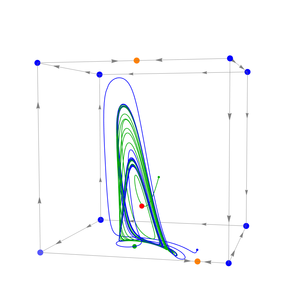
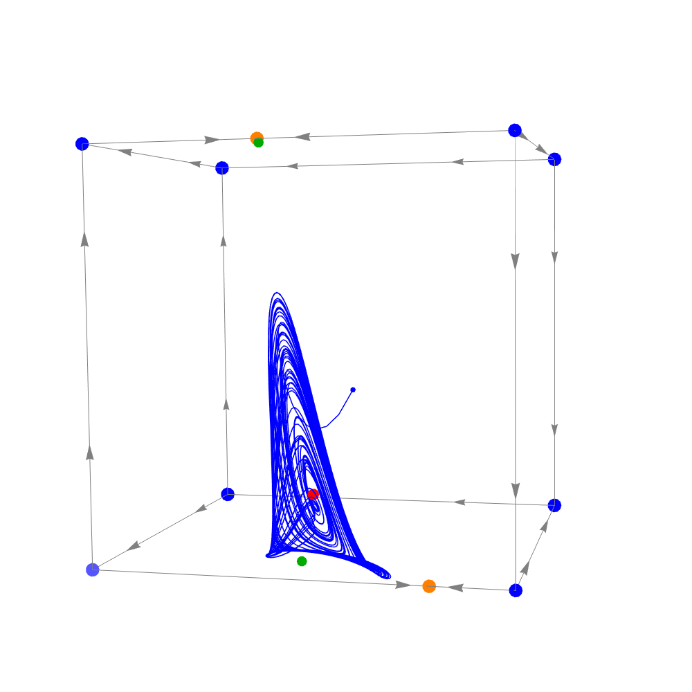
Figure 15. Switching from regular (Case V) to complex (Case VI) dynamics: plot of two orbits (left) and one orbit (right), the interior equilibrium, and all the boundary equilibria of system (6), for $\boldsymbol{\mu}=1.1$ (left) and $\boldsymbol{\mu}=3.6$ (right) with $t\in[0,100]$.

The value $\boldsymbol{\mu}=\boldsymbol{\mu}_{\textrm{SA}}$ seems to be the parameter which separates regular (zero topological entropy) from chaotic dynamics. Before going into Case VI, notice that $W^{s}(A_{2})$ is contained in face $\sigma_{5}$.

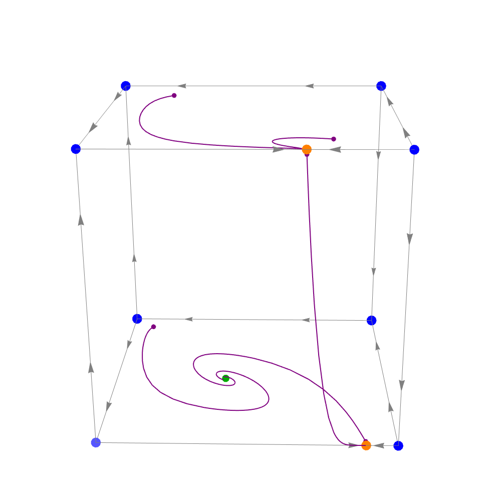
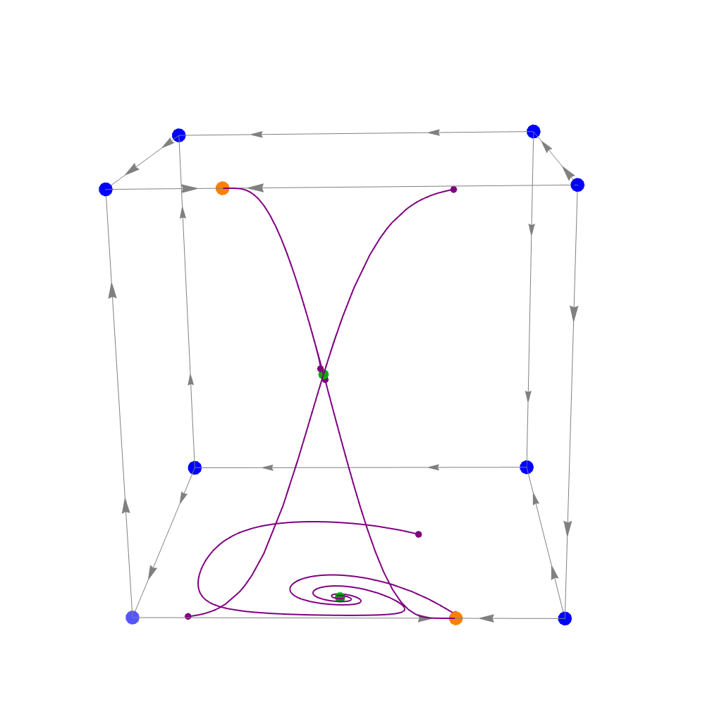
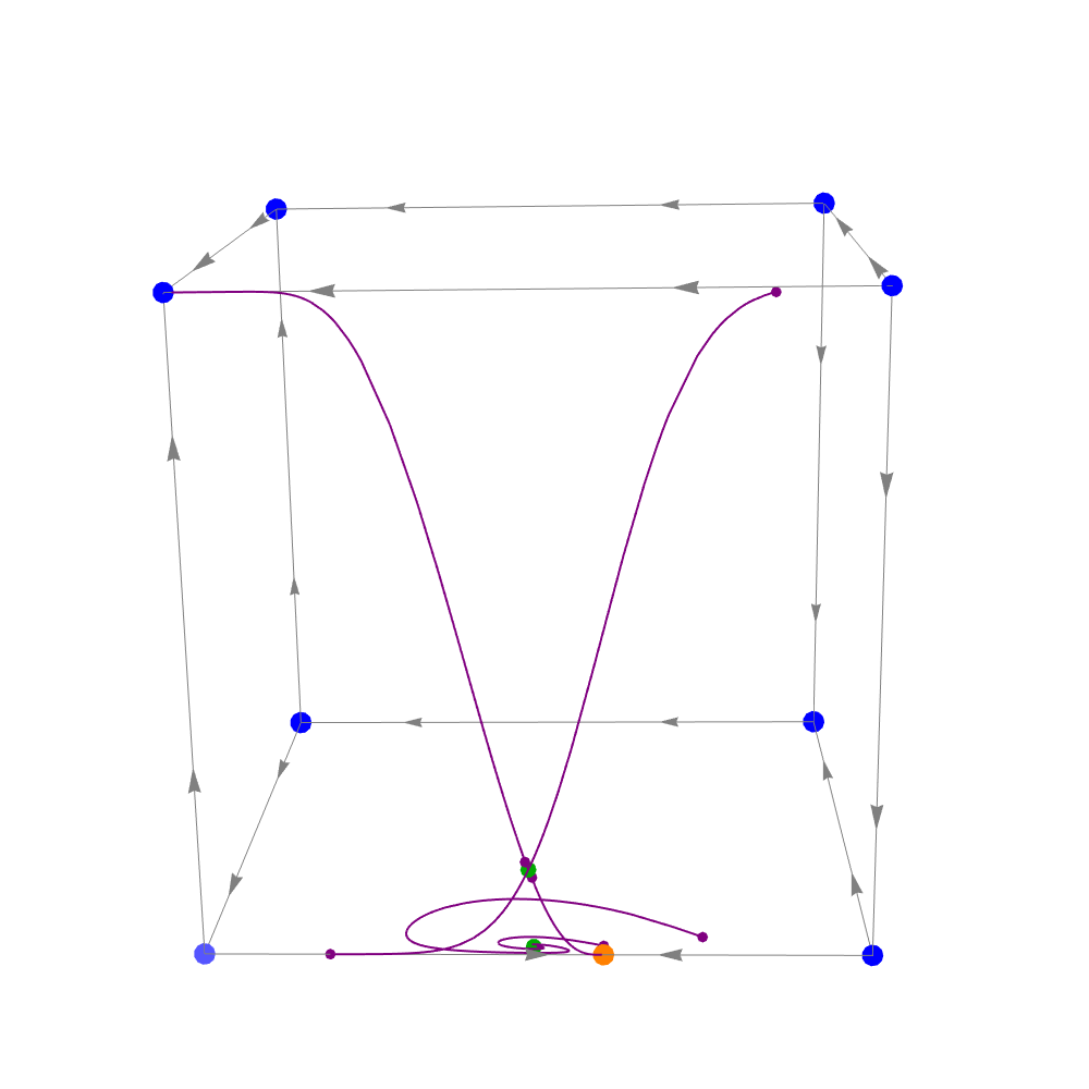
Figure 16. Dynamics on the boundary in Cases V, VI and VII: illustration of the dynamics on the boundary in Cases V (left, $\boldsymbol{\mu}=-5$), VI (center, $\boldsymbol{\mu}=6$) and VII (right, $\boldsymbol{\mu}=9$).

Proposition 11.

In Case VI, the set $\overline{W^{s}(B_{1})}$ contains the points $v_{1}$, $v_{3}$, $v_{5}$, $v_{6}$, $v_{7}$ and $B_{1}$. The set $[0,1]^{3}\backslash\overline{W^{s}(B_{1})}$ has two connected components: in one, the equilibrium $A_{2}$ is a sink; the other is dominated by the non-wandering set associated to a homoclinic orbit to $\mathcal{O}_{\boldsymbol{\mu}}$ for the values of $\boldsymbol{\mu}$ such that the greatest LE of $f_{\boldsymbol{\mu}}$ is positive.

Proof.

The proof of this result comes from a continuity analysis of Case V and Facts  3 and 4. In ${\rm int}\left(\sigma_{4}\right)$, $B_{1}$ is a hyperbolic saddle and Lebesgue almost all points are attracted to either $A_{2}$ or $A_{3}$ as depicted in Figure 16 (center). Since, in Case V, $W^{\textrm{s}}(A_{2})\cap{\rm int}\left(\sigma_{5}\right)={\rm int}\left(\sigma_{5}\right)$ and the equilibrium $B_{1}$ comes from $A_{2}$ through a transcritical bifurcation (see Figure 15 (right)), it turns out that, in Case VI, $W^{\textrm{s}}(B_{1})\,\cap\,{\rm int}\left([0,1]^{3}\right)$ is a two-dimensional invariant manifold whose shape is governed by the internal dynamics that divides the ${\rm int}\left([0,1]^{3}\right)$ in two connected components: the one whose solutions have $\omega$-limit equal to $A_{2}$, and the one that contains the interior equilibrium $\mathcal{O}_{\boldsymbol{\mu}}$. By the same argument as in the proof of Proposition 10, the last assertion follows.

∎

Proposition 12.

In Case VII, the set $\overline{W^{s}(B_{1})}$ contains the points $v_{1}$, $v_{3}$, $v_{6}$, $v_{7}$ and $B_{1}$. The set $\Gamma_{(2,2,2)}\backslash\overline{W^{s}(B_{1})}$ has two connected components: in one the equilibrium $v_{2}$ is a global sink; in the other, we have two sub-Cases:

1. in Case $\textup{VII}.1$, for the values of $\boldsymbol{\mu}$ such that the greatest LE of $f_{\boldsymbol{\mu}}$ is positive, $f_{\boldsymbol{\mu}}$ is $C^{2}$-close to a vector field exhibiting strange attractors.

2. in Case $\textup{VII}.2$, $\mathcal{O}_{\boldsymbol{\mu}}$ is a global sink.

Proof.

The proof of this result replicates that of Proposition 10, except that equilibrium $A_{2}$ no longer exists (see Figure 16 (right)). Notice also that the value of separation between Cases $\textup{VII}.1$ and $\textup{VII}.2$ is $\boldsymbol{\mu}=\boldsymbol{\mu}^{2}_{\textrm{Hopf}}$, responsible for the disappearance of $\mathcal{C}_{\boldsymbol{\mu}}$. From this parameter value on, the proximity of the homoclinic cycle referred in Fact 3 is no longer valid (see Figure 7), and $\mathcal{O}_{\boldsymbol{\mu}}$ becomes stable.

At $\boldsymbol{\mu}=10$, the point $B_{1}$ collapses to $A_{3}$, meaning that volume of the connected component containing $\mathcal{O}_{\boldsymbol{\mu}}$ is shrinking and collapses to a point. In fact, at $\boldsymbol{\mu}=10$, the points $B_{1},B_{2}$ and $\mathcal{O}_{\boldsymbol{\mu}}$ collapse to $A_{3}$ (see $\boldsymbol{\mu}=6.5$ and $\boldsymbol{\mu}=8$ in Table 7).

∎

In Cases VI and VII.1, $\overline{W^{s}(B_{1})}$ plays the role of separatrix: in one component, the $\omega$-limit is either $A_{2}$ (if it exists) or $v_{2}$ (if $A_{2}$ does not exist); in the other, the $\omega$-limit is a strange attractor or a limit cycle (see $\boldsymbol{\mu}=3.6$ and $\boldsymbol{\mu}=6.5$ in Table 7).

7. Proof of Theorem A

Recall, from Subsection 5.2, that $I\subset\left]\boldsymbol{\mu}_{\textrm{SA}},\boldsymbol{\mu}^{2}_{\textrm{Hopf}}\right[$ is a non-degenerate interval of $\boldsymbol{\mu}$-values for which the greatest LE of $f_{\boldsymbol{\mu}}$ is positive (cf. Figure 7).

By Fact 5, there exists an arbitrarily small neighbourhood $\mathcal{U}\subset\mathcal{X}$ of $f_{{\boldsymbol{\mu}}},{\boldsymbol{\mu}}\in I$ and $g\in\mathcal{U}$ such that the flow of $g$ exhibits a homoclinic orbit to the hyperbolic continuation of $\mathcal{O}_{{\boldsymbol{\mu}}}$ (in the $C^{2}$-topology). The eigenvalues of $Df_{{\boldsymbol{\mu}}}\left(\mathcal{O}_{{\boldsymbol{\mu}}}\right)$ have the form described in Fact 2. Reversing the time, the previous configuration gives rise to a flow exhibiting a homoclinic cycle associated to the hyperbolic continuation of $\mathcal{O}_{{\boldsymbol{\mu}}}$, say $\gamma$, whose eigenvalues satisfy the conditions stated in [24, Theorem 1.4].

Define now a one-parameter family of vector fields $(g_{\boldsymbol{\lambda}})_{\boldsymbol{\lambda}\in[-1,1]}\in\mathcal{U}$ unfolding $g$ generically such that:

• $g_{0}\equiv g$ and

• the invariant manifolds associated to the interior equilibrium split with non-zero speed with respect to $\boldsymbol{\lambda}$.

Let $\mathcal{T}$ be a small tubular neighbourhood of the cycle $\gamma$ and $\Sigma$ a cross section to $\gamma$. As illustrated in Figure 17, for $\boldsymbol{\lambda}\in[-1,1]$, let us denote by $\Pi_{\boldsymbol{\lambda}}$ the first return map to the compact cross section $\Sigma\cap\mathcal{T}$, associated to the flow of $g_{\boldsymbol{\lambda}}$.

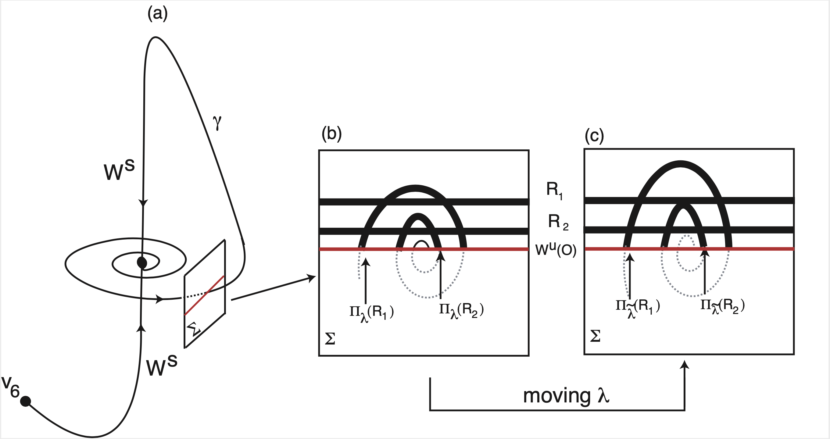
Figure 17. The homoclinic cycle $\gamma$: scheme and shape of the first return map to the cross section $\Sigma$ for the associated to the flow of $g_{\boldsymbol{\lambda}}$, for different values of $\boldsymbol{\lambda}\in[-1,1]$ (b and c). In (b) and (c), the image, under the first return map, of the two horizontal rectangles $R_{1}$ and $R_{2}$ overlap the original rectangles.

Following Shilnikov et al [33], there exists a $\Pi_{0}$-invariant set of initial conditions $\Lambda_{0}\subset\Sigma$ on which the map $\Pi_{0}$ is topologically conjugate to a full shift over an infinite number of symbols. By Gonchenko et al [34], the set $\Lambda_{0}$ contains a sequence of hyperbolic horseshoes $(\mathcal{H}_{n})_{n\in{\mathbb{N}}}$ that are heteroclinically related: the unstable manifolds of the periodic orbits in $\mathcal{H}_{n}$ are long enough to intersect the stable manifolds of the periodic points of $\mathcal{H}_{m}$ (cf Figure 18), for $n,m\in{\mathbb{N}}$. In other words, there exist periodic solutions jumping from a strip of $\mathcal{H}_{n}$ to another strip of $\mathcal{H}_{m}$. For $\boldsymbol{\lambda}\neq 0$, the homoclinic orbit $\gamma$ is broken, but finitely many horseshoes survive. We now use the following result:

Proposition 13 ([16, 35](adapted)).

With respect to the family of maps $(\Pi_{\boldsymbol{\lambda}})_{\boldsymbol{\lambda}\in[-1,1]}$, homoclinic tangencies associated to a dissipative periodic point are dense in $[-1,1]$.

Therefore, for infinitely many parameters $\boldsymbol{\lambda}\in[-1,1]$ we may find a dissipative periodic point $c_{1}\in\mathcal{H}_{n}$, $n\in{\mathbb{N}}$, so that its stable and unstable manifolds have a homoclinic tangency. This tangency is quadratic and breaks generically. Although the original tangencies are destroyed, when the parameter $\boldsymbol{\lambda}$ varies, new tangencies arise nearby. The family $(\Pi_{\boldsymbol{\lambda}})_{{\boldsymbol{\lambda}}}$ may be seen an unfolding of a map exhibiting a quadratic homoclinic tangency; thus one can apply the results by Mora and Viana [17], which guarantee the existence of a positive Lebesgue measure set $E\subset[-1,1]$ of parameter values such that for $\boldsymbol{\lambda}\in E$ the diffeomorphism $\Pi_{\boldsymbol{\lambda}}$ exhibits a Hénon-type strange attractor near the orbit of tangency. Theorem A is proved.

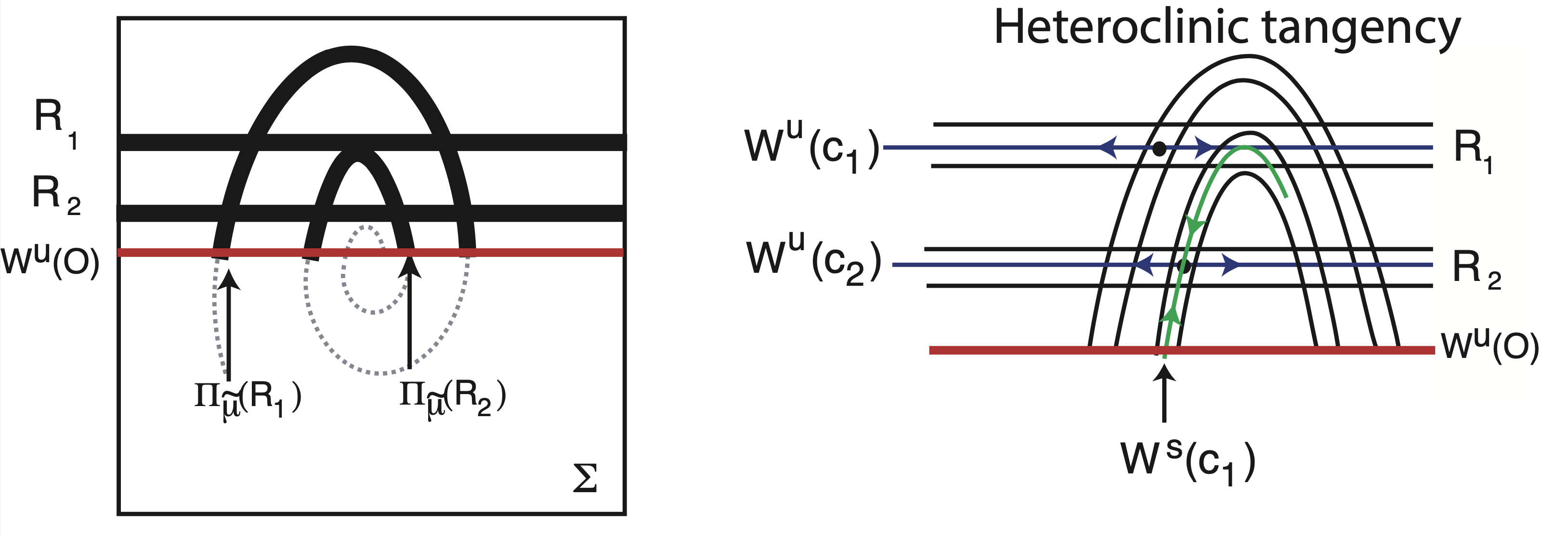
Figure 18. Whiskers of the horseshoes: sketch of the heteroclinic tangencies associated to two saddles associated to the horseshoe $\Lambda_{0}$. The homoclinic classes associated to the horseshoes are not disjoint.

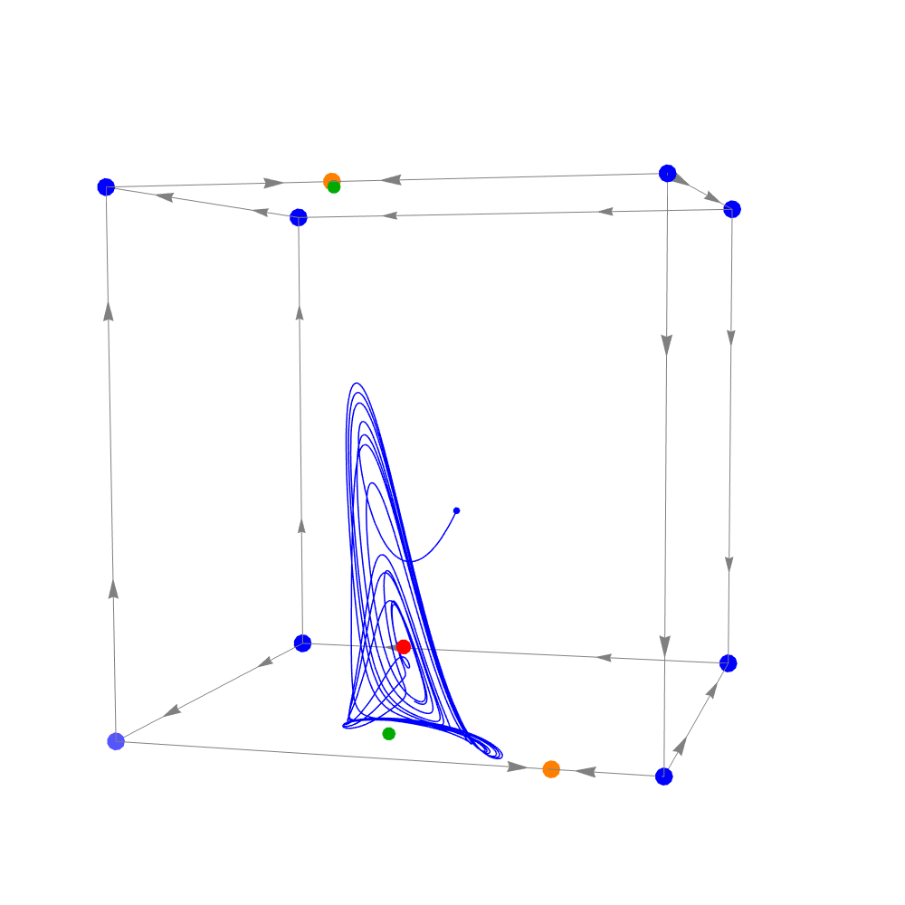
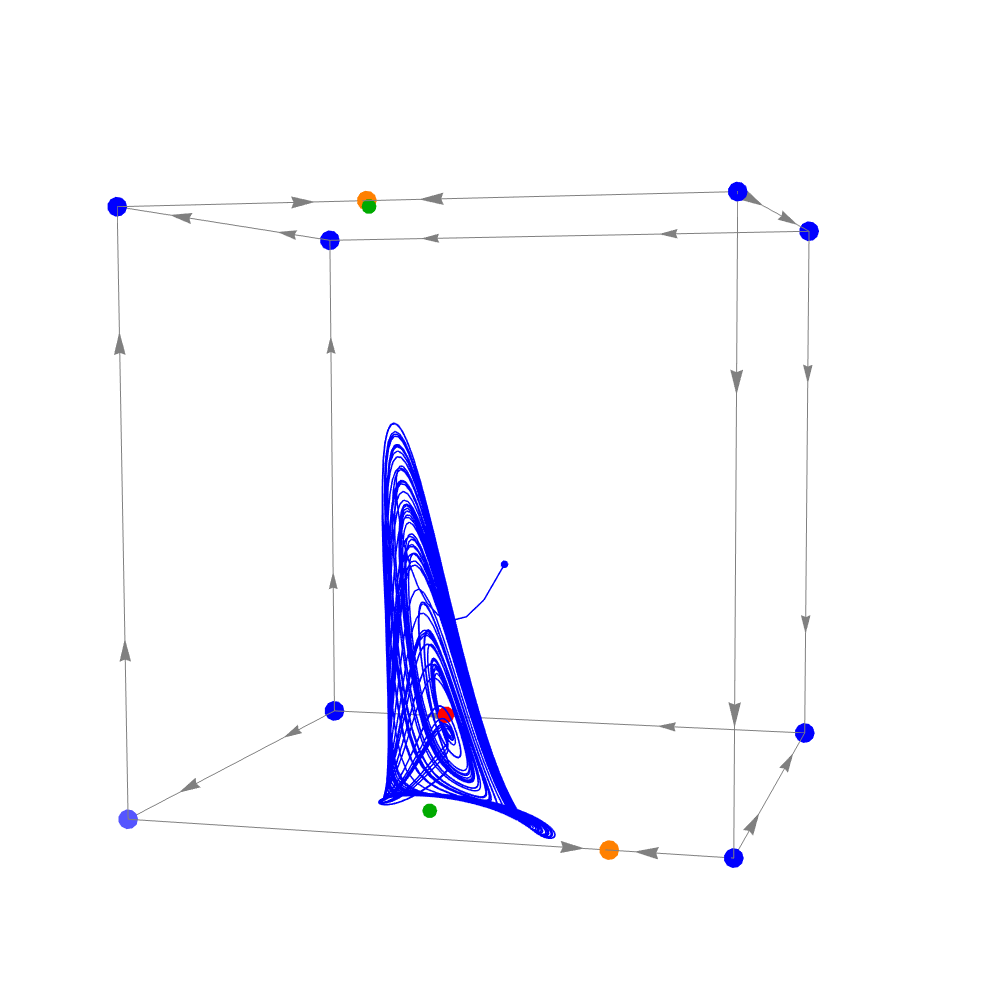
Figure 19. Strange attractor: plot of one orbit (in blue), the interior equilibrium (in red), and all the boundary equilibria (in the corresponding colors) of system (6), for $\boldsymbol{\mu}=3.6$ with $t\in[0,40]$ (left), and $t\in[0,170]$ (right).

Remark.

Besides the existence of strange attractors in the family $(g_{\boldsymbol{\lambda}})_{\boldsymbol{\lambda}\in[-1,1]}$, we may apply Newhouse’s results in the version for one-parameter families [32, Appendix 4], and conclude the existence of infinitely many values of $\boldsymbol{\lambda}\in[-1,1]$ for which the associated flow exhibits a sink.

8. Discussion

In this section, we describe the phenomenological scenario behind the formation of strange attractors for the differential equation (6), relating it with others in the literature.

8.1. Attracting whirlpool: a phenomenological description

We describe the phenomenological scenario responsible for the appearance of the strange attractor of Theorem A. We go back to the works [33, 36] where a similar scenario was proposed for one-parameter families of three-dimensional flows in the context of an atmospheric model.

At $\mu=\boldsymbol{\mu}_{\textrm{Belyakov}}$, the stable interior equilibrium $\mathcal{O}_{\boldsymbol{\mu}}\in\Sigma_{\mu}$ becomes focal. At $\mu=\boldsymbol{\mu}_{\textrm{Hopf}}>\boldsymbol{\mu}_{\textrm{Belyakov}}$, it undergoes a supercritical Andronov-Hopf bifurcation, becoming an unstable saddle-focus, and a stable invariant curve $\mathcal{C}_{\boldsymbol{\mu}}$ is born in its neighborhood. The two-dimensional unstable invariant manifold of $\mathcal{O}_{\boldsymbol{\mu}}$, $W^{u}(\mathcal{O}_{\boldsymbol{\mu}})\subset\Sigma_{\boldsymbol{\mu}}$, is a topological disc limited by $\mathcal{C}_{\boldsymbol{\mu}}$.

After the emergence of the saddle-focus $B_{3}$ ($\boldsymbol{\mu}>b_{3}$ – see Table 4), the set $\Sigma_{\boldsymbol{\mu}}$ starts rotating around $W^{u}(B_{3})$ due to the complex (non-real) eigenvalues of $Df_{\boldsymbol{\mu}}\left(B_{3}\right)$. When $\boldsymbol{\mu}$ increases further, the periodic solution $\mathcal{C}_{\boldsymbol{\mu}}\subset\Sigma_{\boldsymbol{\mu}}$ approaches the cube’s boundary and winds around $W^{u}(B_{3})$, forming a structure similar to the so-called Shilnikov whirlpool [33, 36]. For the $\boldsymbol{\mu}$ values associated to Cases IV and V, the equilibria $B_{2}$ and $B_{3}$ of this whirlpool are pulled to the face $\sigma_{4}$ and the orbits lying on the connected component of ${\rm int}\left(\Gamma_{(2,2,2)}\right)\backslash\overline{W^{s}(B_{1})}$ containing the interior equilibrium are tightened by this whirlpool. Further increasing $\boldsymbol{\mu}$, the size of the whirlpool decreases, and finally, at $\boldsymbol{\mu}\gtrsim\boldsymbol{\mu}_{\textrm{SA}}$, the set $W^{s}(\mathcal{O}_{\boldsymbol{\mu}})$ is arbitrarily close to the screw manifold $W^{u}(\mathcal{O}_{\boldsymbol{\mu}})$. Fact 5 claims the existence of a homoclinic cycle of Shilnikov type for a vector field $C^{2}$-close to $f_{\boldsymbol{\mu}_{\textrm{SA}}}$. The argument that supports this approximation, explained in Subsection 5.3, is valid for the parameter values in the interval $]\boldsymbol{\mu}_{\textrm{SA}},\boldsymbol{\mu}^{2}_{\textrm{Hopf}}[$ for which the greatest LE of $f_{\boldsymbol{\mu}}$ is positive.

As $\boldsymbol{\mu}$ evolves, $\overline{W^{s}(B_{1})}$ divides the cube in two connected components. The one which contains the strange attractor is shrinking, meaning that the volume of initial conditions which realize chaos is vanishing. In terms of the EGT, this would mean that, although system (6) may exhibit chaos, the initial strategies that realize it are very close and cannot go too far (in an appropriate metric).

Our findings are different from those of [33] in the sense that, in their case, the periodic solution coming from the Hopf Bifurcation becomes focal, playing the role of “our” saddle-focus $B_{3}$.

This type of mechanisms, the so called whirlpool attractor may be seen as the universal scenario for the formation of Shilnikov cycles in a typical system [37] – see for example the Rossler model and the “new” Lorenz two-parameter model [36, Section 5].

8.2. Open problem

Simulations with $\textit{Mathematica Wolfram}^{\circledR}$ suggest the existence of a homoclinic orbit to $\mathcal{O}_{\boldsymbol{\mu}}$, for $\boldsymbol{\mu}\approx\boldsymbol{\mu}_{SA}$ and $\boldsymbol{\mu}\approx 3.6$. Nevertheless, for the same parameter values, the homotopy method used by MatCont indicates that the invariant manifolds of $\mathcal{O}_{\boldsymbol{\mu}}$ are close but do not touch. This is why, we have assumed in Fact 5 the existence of a vector field exhibiting a homoclinic nearby. It is an open problem to prove whether the Shilnikov homoclinic orbit exists in the family $\left(f_{\boldsymbol{\mu}}\right)_{\boldsymbol{\mu}}$, however its arbitrary proximity to an element of the family $\left(f_{\boldsymbol{\mu}}\right)_{\boldsymbol{\mu}}$ is enough to trap the observable chaotic dynamics. We conjecture that, up to a change of coordinates, the families $(g_{\boldsymbol{\lambda}})_{\boldsymbol{\lambda}}$ and $(f_{\boldsymbol{\mu}})_{\boldsymbol{\mu}}$ coincide. We are trying hard to find out an answer for this problem.

8.3. Final Remark

We introduced a one-parameter family of polymatrix replicators defined on $\Gamma_{(2,2,2)}$ and study its bifurcations in detail. In an open interval of the parameter space, we prove the existence of a vector field, $C^{2}$-close to elements of the family $(f_{\boldsymbol{\mu}})_{\boldsymbol{\mu}}$, exhibiting a homoclinic cycle to a saddle-focus, responsible for the emergence of suspended horseshoes and persistent observable chaos (Hénon-type in the sense of [17]). This family is structurally stable in the sense that small perturbations of the non-zero entries of $P_{\boldsymbol{\mu}}$ do not qualitatively change the dynamics.

The mechanism responsible for the emergence of chaos seems to be the same for a large class of examples: we obtain an attracting limit cycle (from a supercritical Hopf bifurcation) limiting the unstable manifold of an unstable focus. The stable manifold of the limit cycle starts winding around a focus and accumulates on the stable manifold of the interior equilibrium, undergoing successive saddle-node and period-doubling bifurcations. This criterion relies on Shilnikov’s results [15]. It creates strange attractors that may be seen as a suspension of Hénon-type diffeomorphisms. In particular, when the parameter varies, on a typical cross section, topological horseshoes emerge linked with sinks [35].

The reduction of a polymatrix replicator to dimension three may be carried out just in two cases, $\Gamma_{(2,2,2)}$ (our model) and $\Gamma_{(3,2)}$ (the population is divided in two groups, one with three available strategies and the other with two). The search of strange attractors in the second case may be performed in the same way as we have done in the present article.

The existence of strange attractors in polymatrix replicators has profound implications in the setting of the EGT. Observable chaos is the result of a strategy evolution in which individuals are constantly changing their plans of action in an unforeseeable way. The existence of chaos for model (1) is relevant to maintain the complexity and diversity of strategies, in particular their high unpredictability [38].

Although a complete understanding of the bifurcation diagram associated to (6) and the mechanisms underlying the dynamical changes is out of reach, we uncover complex patterns for the one-parameter family under analysis, using a combination of theoretical tools and computer simulations.

The dynamics on the interior of the cube is strongly determined by the dynamics on the boundary. A lot more needs to be done before the dynamics of polymatrix replicators is completely understood.

Appendix A Tables

Eq.	Eigenvalues	$\boldsymbol{\mu}$	On edge	On $\sigma_{3}$	On $\sigma_{5}$
$A_{1}$	$\left\{\frac{10(\boldsymbol{\mu}+38)}{14-\boldsymbol{\mu}},\frac{4(5\boldsymbol{\mu}+281)}{\boldsymbol{\mu}-14},\frac{26\left(\boldsymbol{\mu}^{2}-2\boldsymbol{\mu}-168\right)}{-(\boldsymbol{\mu}-14)^{2}}\right\}$	$\left[-\frac{2938}{95},-12\right[$	$-$	$-$	$+$
			On edge	On $\sigma_{4}$	On $\sigma_{5}$
$A_{2}$	$\left\{\frac{6(\boldsymbol{\mu}+6)}{\boldsymbol{\mu}-14},\frac{31\boldsymbol{\mu}-110}{\boldsymbol{\mu}-14},\frac{6\left(\boldsymbol{\mu}^{2}-22\boldsymbol{\mu}+112\right)}{-(\boldsymbol{\mu}-14)^{2}}\right\}$	$\left[-\frac{2938}{95},-6\right[$	$-$	$+$	$+$
		$\{-6\}$	$-$	$+$	$0$
		$\left]-6,\frac{110}{31}\right[$	$-$	$+$	$-$
		$\{\frac{110}{31}\}$	$-$	$0$	$-$
		$\left]\frac{110}{31},8\right[$	$-$	$-$	$-$
			On edge	On $\sigma_{4}$	On $\sigma_{6}$
$A_{3}$	$\left\{\frac{27(\boldsymbol{\mu}-10)}{14-\boldsymbol{\mu}},\frac{10(\boldsymbol{\mu}-10)}{\boldsymbol{\mu}-14},\frac{2\left(\boldsymbol{\mu}^{2}-26\boldsymbol{\mu}+168\right)}{-(\boldsymbol{\mu}-14)^{2}}\right\}$	$\left[-\frac{2938}{95},10\right]$	$-$	$-$	$+$
			On edge	On $\sigma_{3}$	On $\sigma_{6}$
$A_{4}$	$\left\{\frac{4(4\boldsymbol{\mu}+241)}{14-\boldsymbol{\mu}},\frac{2(7\boldsymbol{\mu}+122)}{14-\boldsymbol{\mu}},\frac{22\left(\boldsymbol{\mu}^{2}-6\boldsymbol{\mu}-112\right)}{-(\boldsymbol{\mu}-14)^{2}}\right\}$	$\left[-\frac{2938}{95},-\frac{122}{7}\right[$	$-$	$+$	$-$
		$\{-\frac{122}{7}\}$	$-$	$+$	$0$
		$\left]-\frac{122}{7},-8\right[$	$-$	$+$	$+$

Table 3. Eigenvalues of equilibria $A_{1}$, $A_{2}$, $A_{3}$, and $A_{4}$ for system (6), on the corresponding edges and faces (pointing to the interior), where the signs $(-)$, $(0)$, and $(+)$ mean that the eigenvalues are real negative, zero, or positive, respectively.

Eq.	Eigenvalues	$\boldsymbol{\mu}$	On face	On the interior
$B_{1}$	$\left\{\frac{37(\boldsymbol{\mu}-10)}{\boldsymbol{\mu}+40},z_{1},\bar{z}_{1}\right\}$	$\{\frac{110}{31}\}$    $(B_{1}=A_{2})$	$(-,0)$	$(-)$
		$\left]\frac{110}{31},10\right]$	$(-,+)$	$(-)$
$B_{2}$	$\left\{\frac{95\boldsymbol{\mu}+2938}{2(\boldsymbol{\mu}+86)},z_{2},\bar{z}_{2}\right\}$	$\left[-\frac{2938}{95},b_{2}\right[\cup\left[-12,-6\right[$	$(-,-)$	$(+)$
		$\left[b_{2},-12\right[$	$(-,-)_{\textbf{C}}$	$(+)$
		$\{-6\}$    $(B_{2}=A_{2})$	$(-,0)$	$(+)$
$B_{3}$	$\left\{\frac{109(10-\boldsymbol{\mu})}{2(\boldsymbol{\mu}+86)},z_{3},\bar{z}_{3}\right\}$	$\{-\frac{122}{7}\}$    $(B_{3}=A_{4})$	$(-,0)$	$(+)$
		$\left]-\frac{122}{7},b_{3}\right]$	$(-,-)$	$(+)$
		$\left[b_{3},10\right]$	$(-,-)_{\textbf{C}}$	$(+)$

$$z_{1} =\frac{8700-11240\boldsymbol{\mu}+937\boldsymbol{\mu}^{2}+\sqrt{-7052310000+1872624000\boldsymbol{\mu}+179361400\boldsymbol{\mu}^{2}-34941760\boldsymbol{\mu}^{3}+543169\boldsymbol{\mu}^{4}}}{8(\boldsymbol{\mu}+40)^{2}}$$

$$z_{2} =\frac{3\left(-8084+164\boldsymbol{\mu}+3\boldsymbol{\mu}^{2}+\sqrt{259862416+40284768\boldsymbol{\mu}+1909912\boldsymbol{\mu}^{2}+31704\boldsymbol{\mu}^{3}+169\boldsymbol{\mu}^{4}}\right)}{2(\boldsymbol{\mu}+86)^{2}}$$

$$z_{3} =\frac{-19436+892\boldsymbol{\mu}+13\boldsymbol{\mu}^{2}+\sqrt{-3449723504-16764064\boldsymbol{\mu}+27270168\boldsymbol{\mu}^{2}+906392\boldsymbol{\mu}^{3}+6889\boldsymbol{\mu}^{4}}}{2(\boldsymbol{\mu}+86)^{2}}$$

Table 4. Eigenvalues of equilibria $B_{1}$, $B_{2}$, and $B_{3}$ for system (6), on the corresponding faces and pointing to the interior, where $b_{2}\approx-21.9$ and $b_{3}\approx-14.22$. The signs $(-)$, $(0)$, and $(+)$ mean that the eigenvalues are real negative, zero, or positive, respectively, and $(-,-)_{\textbf{C}}$ means that the eigenvalues are conjugate (non-real) with negative real part.

Eq.	Eigenvalues	$\boldsymbol{\mu}$	Analysis
$v_{1}$	$\left\{-10,27,12-\boldsymbol{\mu}\right\}$	$\left[-\frac{2938}{95},10\right]$	$(-,+,+)$
$v_{2}$	$\left\{-23,-14,8-\boldsymbol{\mu}\right\}$	$\left[-\frac{2938}{95},8\right[$	$(-,-,+)$
		$\{8\}$	$(-,-,0)$
		$\left]8,10\right]$	$(-,-,-)$
$v_{3}$	$\left\{6,38,-8-\boldsymbol{\mu}\right\}$	$\left[-\frac{2938}{95},-8\right[$	$(+,+,+)$
		$\{-8\}$	$(0,+,+)$
		$\left]-8,10\right]$	$(-,+,+)$
$v_{4}$	$\left\{-34,10,-12-\boldsymbol{\mu}\right\}$	$\left[-\frac{2938}{95},-8\right[$	$(-,+,+)$
		$\{-12\}$	$(-,0,+)$
		$\left]-12,10\right]$	$(-,-,+)$
$v_{5}$	$\left\{-27,2,10\right\}$	$\left[-\frac{2938}{95},10\right]$	$(-,+,+)$
$v_{6}$	$\left\{6,6,31\right\}$	$\left[-\frac{2938}{95},10\right]$	$(+,+,+)$
$v_{7}$	$\left\{-14,-16,22\right\}$	$\left[-\frac{2938}{95},10\right]$	$(-,-,+)$
$v_{8}$	$\left\{-10,20,26\right\}$	$\left[-\frac{2938}{95},10\right]$	$(-,+,+)$

Table 5. Real eigenvalues of the vertices $v_{1},\dots,v_{8}$ for system (6), where $(-)$, $(0)$, and $(+)$ mean that they are negative, zero, or positive, respectively.

Appendix B Summarizing movie of the boundary dynamics

$(\textup{I})$	$(\textup{II})$	$(\textup{III})$
$\boldsymbol{\mu}\in\left[-\frac{2938}{95},-\frac{122}{7}\right]$	$\boldsymbol{\mu}\in\left]-\frac{122}{7},-12\right]$	$\boldsymbol{\mu}\in\left]-12,-8\right]$
$(\textup{IV})$	$(\textup{V})$	$(\textup{VI})$
$\boldsymbol{\mu}\in\left]-8,-6\right]$	$\boldsymbol{\mu}\in\left]-6,\frac{110}{31}\right]$	$\boldsymbol{\mu}\in\left]\frac{110}{31},8\right]$
$(\textup{VII})$
$\boldsymbol{\mu}\in\left]8,10\right]$

Table 6. Illustration of the dynamics on the cube’s boundary on each interval of $\boldsymbol{\mu}$ in different cases of Table 2.

Appendix C Summarizing movie of the interior dynamics

$\boldsymbol{\mu}=-20$	$\boldsymbol{\mu}=-17.5$	$\boldsymbol{\mu}=-14$
$\boldsymbol{\mu}=-8.5$	$\boldsymbol{\mu}=-7$	$\boldsymbol{\mu}=1.1$
$\boldsymbol{\mu}=3.6$	$\boldsymbol{\mu}=6.5$	$\boldsymbol{\mu}=8$

Table 7. Illustration of the dynamics on the cube’s interior for different values of $\boldsymbol{\mu}$.

References

- [1] Hassan Najafi Alishah and Pedro Duarte. Hamiltonian evolutionary games. Journal of Dynamics & Games, 2(1):33, 2015.
- [2] Hassan Najafi Alishah, Pedro Duarte, and Telmo Peixe. Conservative and dissipative polymatrix replicators. Journal of Dynamics & Games, 2(2):157, 2015.
- [3] Peter Schuster and Karl Sigmund. Coyness, philandering and stable strategies. Animal Behaviour, 29(1):186–192, 1981.
- [4] Peter Schuster, Karl Sigmund, Josef Hofbauer, and Robert Wolff. Self-regulation of behaviour in animal societies. ii. games between two populations without self-interaction. Biological Cybernetics, 40(1):9–15, 1981.
- [5] Manuela AD Aguiar. Is there switching for replicator dynamics and bimatrix games? Physica D: Nonlinear Phenomena, 240(18):1475–1488, 2011.
- [6] Hassan Najafi Alishah, Pedro Duarte, and Telmo Peixe. Asymptotic Poincaré maps along the edges of polytopes. Nonlinearity, 33(1):469, 2019.
- [7] John Maynard Smith and George Robert Price. The logic of animal conflict. Nature, 246(5427):15–18, 1973.
- [8] Brian Skyrms. Chaos and the explanatory significance of equilibrium: Strange attractors in evolutionary game dynamics. In PSA: Proceedings of the Biennial Meeting of the Philosophy of Science Association, volume 2, pages 374–394. Philosophy of Science Association, 1992.
- [9] Steve Smale. On the differential equations of species in competition. Journal of Mathematical Biology, 3(1):5–7, 1976.
- [10] Alain Arneodo, Pierre Coullet, Jean Peyraud, and Charles Tresser. Strange attractors in volterra equations for species in competition. Journal of Mathematical Biology, 14(2):153–157, 1982.
- [11] JA Vano, JC Wildenberg, MB Anderson, JK Noel, and JC Sprott. Chaos in low-dimensional Lotka–Volterra models of competition. Nonlinearity, 19(10):2391, 2006.
- [12] Alain Arneodo, Pierre Coullet, and Charles Tresser. Occurrence of strange attractors in three-dimensional Volterra equations. Physics Letters A, 79(4):259–263, 1980.
- [13] Pablo G Barrientos, Santiago Ibá nez, Alexandre A Rodrigues, and José A Rodríguez. Emergence of Chaotic Dynamics from Singularities, 32th Brazilian Mathematics Colloquium. Instituto Nacional de Matemática Pura e Aplicada (IMPA), 2019.
- [14] Elvio Accinelli, Filipe Martins, Alberto A Pinto, Atefeh Afsar, and Bruno MPM Oliveira. The power of voting and corruption cycles. The Journal of Mathematical Sociology, pages 1–24, 2020.
- [15] Leonid Pavlovich Shilnikov. A case of the existence of a denumerable set of periodic motions. In Doklady Akademii Nauk, volume 160, pages 558–561. Russian Academy of Sciences, 1965.
- [16] Ivan M Ovsyannikov and Leonid Pavlovich Shilnikov. On systems with a saddle-focus homoclinic curve. Matematicheskii Sbornik, 172(4):552–570, 1986.
- [17] Leonardo Mora and Marcelo Viana. Abundance of strange attractors. Acta mathematica, 171(1):1–71, 1993.
- [18] Telmo Peixe. Lotka-Volterra Systems and Polymatrix Replicators. ProQuest LLC, Ann Arbor, MI, 2015. Thesis (Ph.D.)–Universidade de Lisboa (Portugal).
- [19] Telmo Peixe. Permanence in polymatrix replicators. Journal of Dynamics & Games, page 0, 2019.
- [20] John Guckenheimer and Philip Holmes. Nonlinear oscillations, dynamical systems, and bifurcations of vector fields, volume 42. Springer Science & Business Media, 2013.
- [21] Michael J Field. Lectures on bifurcations, dynamics and symmetry. CRC Press, 2020.
- [22] Marco Sandri. Numerical calculation of Lyapunov exponents. Mathematica Journal, 6(3):78–84, 1996.
- [23] Valery Iustinovich Oseledec. A multiplicative ergodic theorem. liapunov characteristic number for dynamical systems. Trans. Moscow Math. Soc., 19:197–231, 1968.
- [24] Ale Jan Homburg. Periodic attractors, strange attractors and hyperbolic dynamics near homoclinic orbits to saddle-focus equilibria. Nonlinearity, 15(4):1029, 2002.
- [25] Dhooge A., W. Govaerts, Y. A. Kuznetsov, Meijer H. G. E., and B. Sautois. New features of the software matcont for bifurcation analysis of dynamical systems. MCMDS, 14(2):147–175, 2008.
- [26] Pablo Aguirre, Bernd Krauskopf, and Hinke M Osinga. Global invariant manifolds near a shilnikov homoclinic bifurcation. Journal of Computational Dynamics, 1(1):1, 2014.
- [27] Alan Wolf, Jack B Swift, Harry L Swinney, and John A Vastano. Determining Lyapunov exponents from a time series. Physica D: Nonlinear Phenomena, 16(3):285–317, 1985.
- [28] AV Andreev, AG Balanov, TM Fromhold, MT Greenaway, AE Hramov, Weibin Li, VV Makarov, and AM Zagoskin. Emergence and control of complex behaviors in driven systems of interacting qubits with dissipation. npj Quantum Information, 7(1):1–7, 2021.
- [29] Anatole Katok. Lyapunov exponents, entropy and periodic orbits for diffeomorphisms. Publications Mathématiques de l’Institut des Hautes Études Scientifiques, 51(1):137–173, 1980.
- [30] J. Hofbauer and K. Sigmund. Evolutionary games and population dynamics. Cambridge university press, 1998.
- [31] Andrea Gaunersdorfer and Josef Hofbauer. Fictitious play, shapley polygons, and the replicator equation. Games and Economic Behavior, 11(2):279–303, 1995.
- [32] Jacob Palis, Jacob Palis Júnior, and Floris Takens. Hyperbolicity and sensitive chaotic dynamics at homoclinic bifurcations: Fractal dimensions and infinitely many attractors in dynamics, volume 35. Cambridge University Press, 1995.
- [33] Leonid Pavlovich Shilnikov. The bifurcation theory and quasi-hyperbolic attractors. Uspehi Mat. Nauk, 36:240–241, 1981.
- [34] Sergey V Gonchenko, Leonid P Shil’nikov, and Dmitry V Turaev. Dynamical phenomena in systems with structurally unstable Poincaré homoclinic orbits. Chaos: An Interdisciplinary Journal of Nonlinear Science, 6(1):15–31, 1996.
- [35] Sheldon E Newhouse. Diffeomorphisms with infinitely many sinks. Topology, 13(1):9–18, 1974.
- [36] Andrey Shil’Nikov, Grégoire Nicolis, and Catherine Nicolis. Bifurcation and predictability analysis of a low-order atmospheric circulation model. International Journal of Bifurcation and Chaos, 5(06):1701–1711, 1995.
- [37] Leon O Chua, Leonid P Shilnikov, Andrey L Shilnikov, and Dmitry V Turaev. Methods Of Qualitative Theory In Nonlinear Dynamics (Part II), volume 5. World Scientific, 2001.
- [38] Kunihiko Kaneko. Chaos as a source of complexity and diversity in evolution. Artificial Life, 1(1_2):163–177, 1993.