A bi-metric universe with matter

Abstract

We analyze the early stage of evolution of a universe with two scale factors proposed in Falomir et al. (2017) when matter is present. The scale factors describe two causally disconnected patches of the universe interacting trough a non-trivial Poisson bracket structure in the momentum sector characterized by one parameter $\kappa$. We studied two scenarios in which one of the patches is always filled with relativistic matter while the other contains relativistic matter in one case, and non-relativistic matter in the second case. By solving numerically the set of equations governing the dynamics, we found that the energy content of one sector drains to the other and from here it is possible to constraint the deformation parameter $\kappa$ by imposing that the decay of the energy density happens, at most, at the Big Bang Nucleosynthesis temperature in order to return to the usual behavior of radiation. The relation with Non Standard Cosmologies is also addressed.

I Introduction

Our present description of the universe rests on the cosmological principle – the hypotheses of spatial homogeneity and isotropy at large scales – described by a Friedman-Lemaitre-Robertson-Walker (FLRW) metric Weinberg (2008); Kolb and Turner (1990). Observations of rotational curves of galaxies Zwicky (1933); Freeman (1970) (for a review see Bertone and Hooper (2018); Salucci (2018)) as well as the observed accelerated cosmic expansion Riess et al. (1998); Perlmutter et al. (1999), made necessary to complete the model with two extra hypothesis: the existence of dark matter and dark energy (cosmological constant term $\Lambda$), respectively. Thus, our present model of the universe, according to observations Zyla et al. (2020), contains a $68,3\%$ of dark energy, $26.8\%$ of cold (non-relativistic) dark matter and $4.9\%$ of baryonic matter.

On the other hand, possible traces of inhomogeneities have been smoothed out during the exponentially accelerated period of expansion known as inflation Peebles and Vilenkin (1999); Linde (1990), a new hypothesis which also solves the flatness and horizon problems, explains the origin of large-scale structures in the universe and restores homogeneity inside the cosmological horizon.

In this regard, in a recent set of papers Falomir et al. (2017, 2018, 2020) a model for a universe with two metrics was considered. In such model, two regions (patches) causally disconnected after the inflation era, are described with metrics of FLRW type with different scale factors for each patch, and a sort of interaction was introduced through a deformation of the Poisson bracket structure in the space of fields. It was shown that, in absence of matter, this sort of interaction emulates the presence of cosmological constant on each patch.

In the present paper we extend the previous model in order to incorporate matter assuming that matter evolves independently on each sector and it can be modelled as a barotropic perfect fluid. We will show that this model can be understood as a sort of Non Standard Cosmology (NSC) Scherrer and Turner (1985); Hamdan and Unwin (1996); Giudice et al. (2001); Gelmini and Gondolo (2006); Maldonado and Unwin (2019); Arias et al. (2019); Bernal et al. (2019), for different values of the parameter controlling the Poisson’s bracket deformation.

In order to do that, in the next section we will show the main features of the model with two metrics and the NSC scenario. Section III is devoted to the discussion of how to incorporate matter into the model. In section IV two cases will be addressed: a) one patch filled with relativistic matter while the second one contains a non-relativistic fluid and b) both patches containing relativistic matter. In the final section we present the conclusions and discuss possible extensions of the model.

II The two-metric universe

The model discussed in Falomir et al. (2017) (see also Falomir et al. (2018, 2020)) describes two patches of the universe through scale factors $a(t)$ an $b(t)$ and a Hamiltonian

$$H = \frac{NG}{2}\left[\frac{\pi_{a}^{2}}{a}+\frac{1}{G^{2}}\left(a\,k_{a}-\frac{\Lambda_{a}}{3}a^{3}\right)\right]+$$ (1)

$$\frac{NG}{2}\left[\frac{\pi_{b}^{2}}{b}+\frac{1}{G^{2}}\left(b\,k_{b}-\frac{\Lambda_{b}}{3}b^{3}\right)\right],$$

$$\equiv H_{a}+H_{b}$$ (2)

where $\pi_{a},\pi_{b}$ are the conjugate momenta of $a$ and $b$, respectively. Scale factors are chosen with canonical dimension $-1$ and then, momenta have dimension +1. $N$ is an auxiliary field that guaranties the time reparametrization invariance. Patches $a$, $b$ have spatial curvature $k_{a}$, $k_{b}$ and cosmological constant $\Lambda_{a},\Lambda_{b}$, respectively.

The Poisson bracket structure, on the other hand, is defined through the following relations

$$\{a_{\alpha},a_{\beta}\}=0,\quad\{a_{\alpha},\pi_{\beta}\}=\delta_{\alpha\beta},\quad\{\pi_{\alpha},\pi_{\beta}\}=\theta\,\epsilon_{\alpha\beta},$$ (3)

with $\theta$ a constant parameter and index $\{\alpha,\beta\}\in\{a,b\}$. Scale factors notation is $a_{a}=a,a_{b}=b$. It is convenient to redefine the parameter $\theta$ as $\theta=\kappa\,G^{-1}$ with $\kappa$ a dimensionless parameter.

Equations of motion derived from Hamiltonian (1) with Poisson brackets (3) are

$$\dot{a} = G\frac{\pi_{a}}{a},\quad\dot{b}=G\frac{\pi_{b}}{b},$$ (4)

$$\dot{\pi}_{a} = G\frac{\pi_{a}^{2}}{2a^{2}}+\frac{1}{2G}\left(a^{2}\Lambda_{a}-k_{a}\right)+\kappa\frac{\pi_{b}}{b},$$ (5)

$$\dot{\pi}_{b} = G\frac{\pi_{b}^{2}}{2b^{2}}+\frac{1}{2G}\left(b^{2}\Lambda_{b}-k_{b}\right)+\kappa\frac{\pi_{a}}{a},$$ (6)

while the constraint $\dot{\pi}_{N}=0$ reads

$$\frac{\pi_{a}^{2}}{a}+\frac{\pi_{b}^{2}}{b}+G^{-2}\left(a\,k_{a}+b\,k_{b}-\frac{\Lambda_{a}}{3}\,a^{3}-\frac{\Lambda_{b}}{3}\,b^{3}\right)=0.$$ (7)

Note that we have written the equations in the usual gauge $N=1$ (equivalently, we have redefined the time variable $dt^{\prime}=N(t)dt$).

Equations (4) to (7) can be recast as the following set of second order differential equations

$$2a\ddot{a}+\dot{a}^{2} = \Lambda_{a}\,a^{2}-k_{a}+2\kappa\dot{b},$$ (8)

$$2b\ddot{b}+\dot{b}^{2} = \Lambda_{b}\,b^{2}-k_{b}-2\kappa\dot{a},$$ (9)

$$a\dot{a}^{2}+b\dot{b}^{2} = \frac{\Lambda_{a}}{3}\,a^{3}-k_{a}\,a+\frac{\Lambda_{b}}{3}\,b^{3}-k_{b}.$$ (10)

The model presents several interesting properties, as for example, the existence of solutions containing both, accelerated and decelerated periods, or the presence of an inflationary epoch in a patch with a negligible cosmological constant (for example, for $\Lambda_{a}\ll\Lambda_{b}$). Note also that the equations are symmetric under the simultaneous change $a\rightarrow b$, $b\rightarrow a$ and $\kappa\rightarrow-\kappa$.

The effect of matter in the model, on the other hand, has not been explored and it is the main purpose of the present work to investigate this scenario. We will show that this two-metric model with matter have similar features compared with the Non Standard Cosmologies (NSCs) scenarios.

Indeed, the study of the effects of different cosmological histories at early stages of the universe, such as matter domination ($H\propto T^{3/2}$) Giudice et al. (2001), kination domination ($H\propto T^{6}$) Visinelli (2018) or even a field with a general state of equation ($H\propto T^{3(\omega+1)/2}$) Maldonado and Unwin (2019); Arias et al. (2019); Bernal et al. (2019), where $H$ is the Hubble parameter, is a very active field of research.

A particular scenario relevant to the present work considers the introduction of a field ($\phi$) whose only effect is to modify the expansion rate of the universe, making it faster or slower (and also can decay into Standard Model particles). These kind of different cosmological histories are usually called Non-Standard Cosmologies (NSCs) and the only restriction for this new field is to decay before the epoch of Big Bang Nucleosinthesys (BBN), in order not to be in conflict with astrophysical measures Chung et al. (1999); Kolb et al. (2003).

For a general NSC model, the evolution equations read

$$\dot{\rho_{\text{SM}}}+4H\rho_{\text{SM}} = \Gamma\rho_{\phi}$$ (11)

$$\dot{\rho_{\phi}}+3(\omega+1)H\rho_{\phi} = -\Gamma\rho_{\phi},$$ (12)

where $\rho_{\text{SM}}$ is the energy density of the Standard Model (SM) content, $\rho_{\phi}$ is the energy density of the new field, $\omega$ is the constant for the barotropic fluid, $\Gamma$ the decay constant for the $\phi$ field and $H$ is the Hubble parameter.

The decay constant $\Gamma$ can be expressed in terms of the re-heating temperature $T_{RH}$ (sometimes called $T_{\text{end}}$ depending on the behavior of the $\phi$ field), by demanding

$$\Gamma=\frac{\pi}{3}\sqrt{\frac{g_{\star}}{10}}T_{RH}^{2},$$ (13)

that is, $\Gamma$ is equal to the value of the Huble parameter at the time when universe is dominated by radiation again. Here, $g_{*}$ is the degrees of freedom of radiation that we will consider as a constant with value $g_{\star}\approx 10$, which corresponds to a temperature for $T_{\text{RH}}$ (or $T_{\text{end}}$) of $T=4\times 10^{-3}$ GeV. This value is imposed by the BBN epoch and corresponds to the lowest value of the temperature at which this new field must decay Kawasaki et al. (2000); Hannestad (2004).

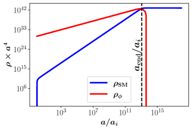
(a)

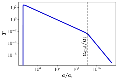
(b)

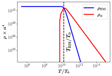
(c)

Figure 1: Panel (a) shows the $\phi$ field acting like an inflaton. The SM sector starts to grow with the evolution of $\phi$ until $T_{RH}=4\times 10^{-3}$ GeV is reached and $\phi$ decays. In panel (b) the temperature as a function of $a/a_{i}$ is shown. The change of slope at $T_{RH}$ is due to the decay of the $\phi$ field. Energy density as function of $T$ is shown in (c), with $T_{0}=2.33\times 10^{-13}$ GeV.

The $\phi$ field has interesting features. It acts like an inflaton when the initial energy density $\rho_{\text{SM}}$ is zero and then, generates a new epoch of reheating due to the decay term which transfers energy to the SM content until $T_{RH}$ is reached Giudice et al. (2001); Maldonado and Unwin (2019). At this temperature the $\phi$ field decays completely. This effect is shown in Figure 1.

For a less restrictive scenario, one assumes a non zero ratio between the energy density of $\phi$ and the energy density of the SM, at some initial scale factor $a_{i}$. That is, a non zero value for the quantity

$$\delta=\frac{\rho_{\phi}}{\rho_{\text{SM}}}\bigg{|}_{a_{i}}.$$

In this case, this new field does not act like an inflaton anymore, but we can observe a similar behavior growing up the energy density for the SM content meanwhile the $\phi$ field is decaying until $T_{\text{end}}$, which is the temperature when total decay occurs Bernal et al. (2019).

It is interesting to note that the two-metric model in absence of matter also shows an inflaton-like behavior Falomir et al. (2017), but there the interaction provided by the deformation of the Poisson bracket structure is the responsible for such effect. We will show that for the matter case, it is possible to reproduce also the behavior shown in Figure 2.

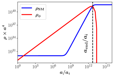
(a)

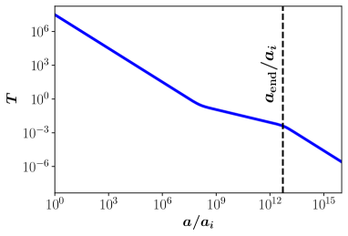
(b)

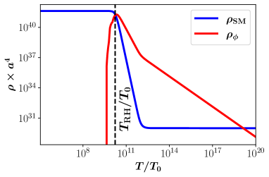
(c)

Figure 2: Panel (a) shows the evolution of energy density of $\phi$ field and the SM bath for $\delta=10^{-1}$. $\Gamma$ is chosen so that $\phi$ decays at $T_{RH}=4\times 10^{-3}$ GeV. Panel (b) exhibits the temperature as a function of $a/a_{i}$. The slope changes due to the effect the $\phi$ field which is decaying. The panel (c) show the relationship between the energy densities and the temperature, with $T_{0}=2.33\times 10^{-13}$ GeV the current temperature.

III The matter content

We are interested in the study of energy density evolution under the hypothesis that the evolution of matter in one patch is independent from the other and particularized to barotropic perfect fluids characterized by the presure $p$ and the energy density $\rho$.

Note that the LHS of (8) and (9) are proportional to the spatial component of the Einstein tensor. Indeed, for a FLRW metric with scale factor $a$ and spatial curvature $k_{a}$ (in the gauge $N=1$) the Einstein tensor reads

$$G_{ij}=-g_{ij}\left(2a\ddot{a}+\dot{a}^{2}+k_{a}\right),\quad G_{00}=\frac{3}{a^{2}}\left(\dot{a}^{2}+\kappa_{a}\right),$$ (14)

and then, under the hypothesis previously explained, we propose the following modification of the equations of motion in order to include matter effects

$$2a\ddot{a}+\dot{a}^{2} = \Lambda_{a}\,a^{2}-k_{a}+2\kappa\dot{b}-a^{2}{p}_{a},$$ (15)

$$2b\ddot{b}+\dot{b}^{2} = \Lambda_{b}\,b^{2}-k_{b}-2\kappa\dot{a}-b^{2}{p_{b}},$$ (16)

$$a\dot{a}^{2}+b\dot{b}^{2} = \frac{\Lambda_{a}}{3}\,a^{3}-k_{a}\,a+\frac{a^{3}}{3}{\rho}_{a}+$$ (17)

$$\frac{\Lambda_{b}}{3}\,b^{3}-k_{b}\,b+\frac{b^{3}}{3}{\rho}_{b},$$

where $p$ and $\rho$ are the pressure and energy density of the fluid (in $M_{\mbox{\tiny{Pl}}}=(8\pi G)^{-1/2}$ units), respectively, and index $a,b$ denotes the patch where they are defined.

A comment is in order here. While the pressure terms in (15) and (16) trivially satisfy the hypothesis of local matter content, modifications of the constraint equation – the term $a^{3}\rho_{a}+b^{3}\rho_{b}$ in (17) – have not a unique form. The most general term modifying (17) must be a function $\rho^{(ab)}$ which satisfies also the separability condition $\rho^{(ab)}=\rho^{(a)}+\rho^{(b)}$, since the constraint in the present model turns out to be the addition of the usual ones on each patch. Indeed, for the FLRW metric with scale factor $a$, constraint reads ${\cal C}_{a}=a\dot{a}^{2}-\frac{\Lambda_{a}}{3}\,a^{3}+k_{a}\,a-\frac{a^{3}}{3}{\rho}_{a}=0$, while for the present two-metric model, the constraint reads ${\cal C}_{a}+{\cal C}_{b}=0$.

Previous characteristic is a consequence of the fact that there is only one time for both patches (and then, only one lapse function $N$) ensuring the time reparametrization invariance. Then, our choice of energy density term respects the separability condition and it reproduces also the standard cosmological scenario if both patches are not connected, that is $\kappa=0$.

The conservation law is obtained by taking the time derivative of the constraint and replacing the second derivatives of the scale factors from (15) and (16). For a general energy-density term $\rho^{(ab)}$ the continuity equation reads

$$\dot{\rho}^{(ab)}+\dot{a}\,a^{2}\,p_{a}+\dot{b}\,b^{2}\,p_{b}=0.$$ (18)

Once we specify the function $\rho^{(ab)}$ to our choice in (17), previous equation turn out to be

$$a^{3}\left[\dot{\rho}_{a}+3H_{a}^{2}\left(\rho_{a}+p_{a}\right)\right]+b^{3}\left[\dot{\rho}_{b}+3H_{b}^{2}\left(\rho_{b}+p_{b}\right)\right] = 0,$$

with $H_{a}=\dot{a}/a$ and $H_{b}=\dot{b}/b$, the Hubble parameters on each patch.

To summarize, in the present approach where matter on patches $a$ and $b$ are characterized by their pressure and energy density (on each patch), the evolution of the scale factors are given by equations (15) to (17) from which the conservation equation (III) follows.

IV Barotropic mater in the early universe

We will analyze the effects of the matter presence for the case in which fluids on $a$ and $b$ satisfy the barotropic condition

$$p_{a}=\omega_{a}\,\rho_{a},\quad p_{b}=\omega_{b}\,\rho_{b}.$$ (20)

In the forthcoming analysis, the contributions from cosmological constant will be neglected since we are interested in the early stage of the evolution of the universe, which is an interesting scenario for different physical phenomena like Dark Matter production Giudice et al. (2001); Maldonado and Unwin (2019); Bernal et al. (2019); Arias et al. (2019) or gravitational waves Bernal et al. (2020), among others. Also, we set $k_{a}=0=k_{b}$, the favored scenario consistent with cosmological data Zyla et al. (2020). Note also that, in spite of the choice $\Lambda_{a}=0=\Lambda_{b}$, a sort of cosmological constant term is always present due to the effects of a non zero value of $\kappa$ Falomir et al. (2017). The equations of evolution, with previous choices, turn out to be

$$2\frac{\ddot{a}}{a}+H_{a}^{2}+\omega_{a}\,\rho_{a} = ~{}2\kappa\,\frac{\dot{b}}{a^{2}},$$ (21)

$$2\frac{\ddot{b}}{b}+H_{b}^{2}+\omega_{b}\,\rho_{b} = -2\kappa\,\frac{\dot{a}}{b^{2}},$$ (22)

$$a^{3}\left[H_{a}^{2}-\frac{1}{3}\rho_{a}\right] + b^{3}\left[H_{b}^{2}-\frac{1}{3}\rho_{b}\right]=0,$$ (23)

while the continuity equation read

$$a^{3} \left[\dot{\rho}_{a}+3\rho_{a}H_{a}^{2}\left(\omega_{a}+1\right)\right]+$$

$$b^{3} \left[\dot{\rho}_{b}+3\rho_{b}H_{b}^{2}\left(\omega_{b}+1\right)\right]=0.$$ (24)

In the present model, we will look for solutions of (23) respecting the separability hypothesis and then, we look for solutions which are also the solutions of

$$H_{a}^{2}-\frac{\rho_{a}}{3} = 0,$$ (25)

$$H_{b}^{2}-\frac{\rho_{b}}{3} = 0.$$ (26)

The time derivative of previous equations give rise to the following conditions

$$a^{3}\left(\dot{\rho}_{a}+3H_{a}(\omega_{a}+1)\rho_{a}\right) = 6\kappa\,\dot{a}\dot{b},$$ (27)

$$b^{3}\left(\dot{\rho}_{b}+3H_{b}(\omega_{b}+1)\rho_{b}\right) = -6\kappa\,\dot{a}\dot{b},$$ (28)

which, when added, turn out to be (IV).

Comparing (27) and (28) with (11) and (12) for the case of NSC, we observe the similar source-sink behavior due to the $\kappa$ term in the two-metric model. However, the decaying constant $\Gamma$ is now time dependent. Moreover, one can rewrite (27) and (28) as

$$\dot{\rho}_{a}+3H_{a}(\omega_{a}+1)\rho_{a} = \Gamma_{a}\,\rho_{b},$$ (29)

$$\dot{\rho}_{b}+3H_{b}(\omega_{b}+1)\rho_{b} = -\Gamma_{b}\,\rho_{b},$$ (30)

with

$$\Gamma_{a}=2\kappa\frac{b}{a^{2}}\,\delta^{-1/2},\quad\Gamma_{b}=2\kappa\frac{a}{b^{2}}\,{\delta^{-1/2}},$$ (31)

and $\delta=\rho_{b}/\rho_{a}$. The decay functions $\Gamma$ satisfy $a^{3}\Gamma_{a}-b^{3}\Gamma_{b}=0$. In this sense, the two-metric model with matter can be understood as an extension of NSC.

In the following sections we will study the numerical solutions of the set of equations (25) to (28) in two cases. For both scenario the energy density in $a$ patch will have a radiation-like barotropic equation so that we can compare with with NSC, (we will refer this content as relativistic) while the patch $b$ contains relativistic matter in one case and non-relativistic, in the other. Even though the numerical solutions found are functions of time, it is convenient to express results in terms of temperatures.

The temperature dependence is incorporated by noticing that in patch $a$, where relativistic matter dominates, the following relation holds

$$\rho_{a}=\frac{\pi^{2}}{30}g_{*}T^{4},$$ (32)

with $g_{*}$ the number of massless degrees of freedom.

IV.1 Patch $b$ filled with non-relativistic matter

In this case, as we previously discussed, patch $a$ is filled with relativistic matter while the energy content of $b$ is non-relativistic. Then $\omega_{a}=1/3$ and $\omega_{b}=0$ and the set of equations (25) to (28) to determine time evolution of scale factors and energy densities are

$$\dot{a} = \sqrt{\frac{\rho_{a}}{3M_{p}^{2}}}\,a,$$

$$\dot{b} = \sqrt{\frac{\rho_{b}}{3M_{p}^{2}}}\,b,$$

$$\dot{\rho}_{a} = -\frac{4}{\sqrt{3M_{p}^{2}}}(\rho_{a})^{3/2}+2\kappa M_{p}\sqrt{\rho_{a}\rho_{b}}\,\frac{b}{a^{2}},$$

$$\dot{\rho}_{b} = -\frac{1}{\sqrt{3M_{p}^{2}}}(\rho_{b})^{3/2}-2\kappa M_{p}\sqrt{\rho_{a}\rho_{b}}\,\frac{a}{b^{2}},$$ (33)

where we have restored the Planck mass constant.

Numerical results for the energy density evolution as function of temperature are shown in Figures 3, 4 and 5. The quantities of interest, as function of temperature, are $\rho\times$(scale factor)^ℓ, for some power $\ell$.

In all cases with $\kappa\neq 0$ we observe a drain effect, namely, the energy density of sector $b$ decrease until it vanishes, while the energy density in $a$ increases. The temperature at which the total drain occurs depends on the value of $\kappa$ as well as the ratio $\delta$ at initial time. This is consistent with the interpretation of source-sink system given by (29).

The dashed line marks the ratio $T_{BBN}/T_{0}$ at which the drain of the energy content of $b$ should end. That is the drain must happen, at most, at the temperatures of the order of the temperature of Big Bang Nucleosynthesis ($T_{BBN}$) or higher than $T_{BBN}$.

The panel (a) in Figure 3 shows the situation for $\kappa=0$ in order to check that the systems are decoupled in such case and the energy densities evolve as it is expected for radiation and non-relativistic matter. Thas is, $\rho_{a}\propto a^{-4}$ and $\rho_{b}\propto b^{-3}$.

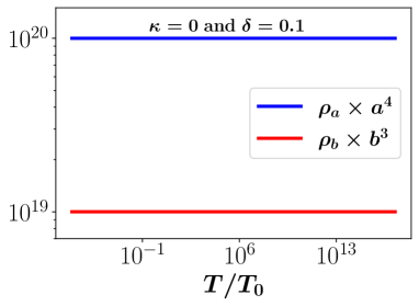
(a)

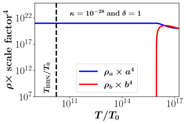
(b)

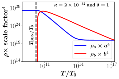
(c)

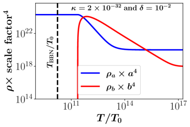
(d)

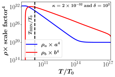
(e)

Figure 3: Evolution of energy density for relativistic matter in $a$ and non-relativistic matter in $b$ as function of the temperature $T/T_{0}$. $T_{0}$ is the CMB temperature at present ($T_{0}=2.33\times 10^{-13}$ GeV). The dashed line indicates the Big Bang Nucleosynthesis temperature at which $\rho_{b}$ should vanish. For all cases the initial density $\rho_{a}=10^{20}$ GeV. Panel (a) shows the case $\kappa=0$. Panels (b) and (c) are the solutions for $\delta=1$ and different values of $\kappa$. The panels (d) and (e) show the evolution for $\delta\neq 1$ and same value of $\kappa$.

Panels (b) and (c) of Figure 3 show the case of initial ratio $\delta=1$ and it is possible to observe that the decay of $b$ happens at higher temperatures (compared with $T_{BBN}$) as $\kappa$ increases. Indeed, it is enough to have $\kappa\gtrsim 10^{-32}$ in order to have a complete decay of energy content of $b$ sector at $T_{BBN}$. This is consistent with the fact that $\Gamma_{a}$ in (29) is proportional to $\kappa$.

Let us take now the value of $\kappa$ so that the total drain occurs at the desired temperature for a symmetric initial density condition ($\delta=1$), situation shown in panel (c). The effect of initial condition $\delta>1$ and $\delta<1$ can be observed in panels (d) and (e) in the same figure. We observe in panel (e) that when $b$ patch has more energy to drain (compared with the energy of $a$ patch) at the initial time, the complete process takes a longer time, so that the total decay of energy in patch $b$ happens at temperatures smaller than $T_{BBN}$, which is an unfavorable scenario.

In all previous cases the initial value of energy density in $a$ is $\rho_{a}=10^{20}$ GeV. The effect of a different initial condition for $\rho_{a}$ has been also addressed and the results are shown in Figures 4 and 5. In the first, the initial value of energy density is $\rho_{a}=10^{10}$ GeV while it is $\rho_{a}=10^{30}$ GeV in the second. For both cases we have chosen $\delta=1$. We conclude that the value of $\kappa$ for which the total drain happens at the desired temperature $T_{BBN}$ decreases as the initial density $\rho_{a}$ decreases, what is consistent with our previous result in Figure 3, panels (b) and (c).

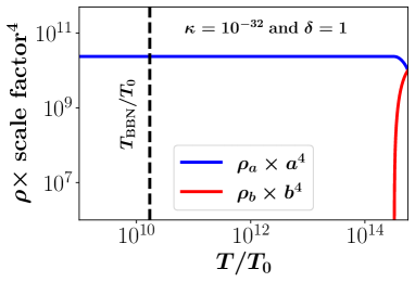
(a)

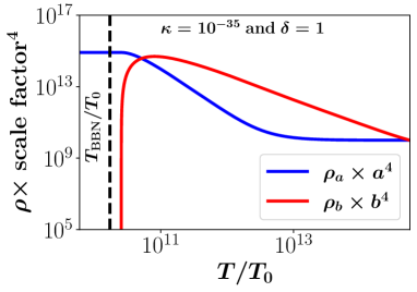
(b)

Figure 4: Evolution of energy density for different values of $\kappa$ and initial condition $\rho_{a}=10^{10}$ GeV with $\delta=1$.

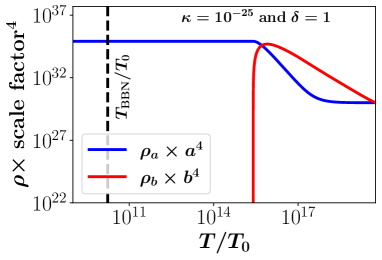
(a)

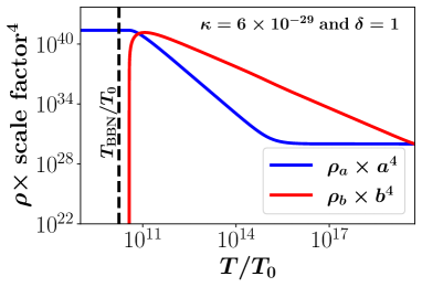
(b)

Figure 5: Evolution of energy density for different values of $\kappa$ and initial condition $\rho_{a}=10^{30}$ GeV with $\delta=1$.

To summarize, the temperature at which the energy density of sector $b$ vanishes, producing an increment of the energy content in sector $a$ (a source-sink effect) depends on the values of $\kappa$, the initial value of the energy density in sector $a$ and $\delta$. Large values of $\kappa$ produces a fast decay of $\rho_{b}$ while large values of initial $\rho_{a}$ slow down the decay rate. For a fixed $\kappa$, instead, large values of initial $\rho_{b}$ also slow down the decay rate.

In the following section we will analyze the case in which the sector $b$ has relativistic matter also and we will show that previous conclusions are also valid for such case.

IV.2 Patch $b$ filled with relativistic matter.

In this case, the patches $a$ and $b$ contain relativistic matter ($\omega_{a}=\omega_{b}=1/3$). The set of equations (25) to (28) to determine time evolution of scale factors and the energy density (with the Planck mass restored) are

$$\dot{a} = \sqrt{\frac{\rho_{a}}{3M_{p}^{2}}}\,a,$$

$$\dot{b} = \sqrt{\frac{\rho_{b}}{3M_{p}^{2}}}\,b,$$

$$\dot{\rho}_{a} = -\frac{4}{\sqrt{3M_{p}^{2}}}(\rho_{a})^{3/2}+2\kappa M_{p}\sqrt{\rho_{a}\rho_{b}}\,\frac{b}{a^{2}},$$

$$\dot{\rho}_{b} = -\frac{4}{\sqrt{3M_{p}^{2}}}(\rho_{b})^{3/2}-2\kappa M_{p}\sqrt{\rho_{a}\rho_{b}}\,\frac{a}{b^{2}}.$$ (34)

The evolution of energy densities as function of temperatures is shown in Figures 6 to 8 for different values of initial $\rho_{a}$ and $\delta=1$.

We observe for all cases how the energy density of relativistic matter in sector $a$ increases at expenses of the energy content of sector $b$ until the energy on this sector is completely drained. For the initial condition $\rho_{a}=10^{10}$ GeV we can compare the relativistic–relativistic case depicted in Figure 6 with the relatvistic–non-relativistic case in Figure 4. Again, for large values of $\kappa$, the total drain occurs for temperatures grater than the BBN temperature. The value of $\kappa$ at which the total drain happens near $T_{BBN}$ is slightly smaller compared with the radiation-matter case.

The effects of a larger initial value of $\rho_{a}$ (with $\delta=1$) are shown in Figures 7 and 8 which should be compared with Figures 3 (panels (b) and (c)) and 5, respectively. The general features previously discussed are observed here and, additionally, a small value of $\kappa$, compared with the relativistic–non-relativistic case, is necessary in order to reach the total drain at $T_{BBN}$. In other words, for a fixed value of $\kappa$ and initial $\delta=1$, the drain of energy from $b$ to $a$ happens faster if $b$ contains radiation compared with the case in which $b$ contains non-relativistic matter.

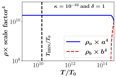
(a)

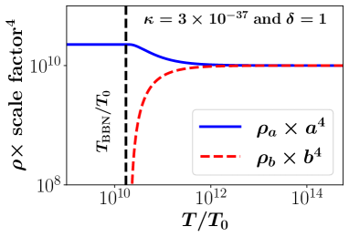
(b)

Figure 6: Evolution of radiation content in patch $a$ and $b$ as function of the temperature. Panels (a) and (b) show the energy densities evolution for an initial condition $\rho_{a}=10^{10}$ GeV and $\delta=1$ and different values of $\kappa$.

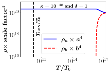
(a)

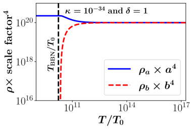
(b)

Figure 7: Evolutution of radiation content in patch $a$ and $b$ as function of the temperature. In the $y$ axes we have plotted $\rho_{a}\times a^{4}$ and $\rho_{b}\times b^{4}$ . Panels (a) and (b) show the energy densities evolution for an initial condition $\rho_{a}=10^{20}$ GeV and $\delta=1$ an different values of $\kappa$

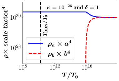
(a)

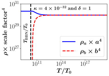
(b)

Figure 8: Radiation content in patch $a$ and $b$ as function of the temperature. Panels (a) and (b) show the energy densities evolution for an initial condition $\rho_{a}=10^{30}$ GeV and $\delta=1$.

V Discussion and Conclusions

In this work we have presented an extension of a cosmological model with two scale factors in order to include matter. The two scale factors might represent two sectors of a universe (two patches) Rasouli et al. (2019), or even two different universes in a multiverse scenario Linde (2017) which are causally connected only through a deformation of the Poisson bracket structure. In this sense, this model is a sort of a non-commutative cosmology. The model is the analogous of the Landau problem in the space of metrics Falomir et al. (2018).

The evolution of matter in such universe have been addressed and, in order to do that, we have assumed a) the matter content on each patch do not interact – our matter-independent hypothesis – and b) the modification of equations of motion is minimal and it reduces to the usual equations of motion of General Relativity when the deformation parameter $\kappa=0$.

Under such hypotheses, the equations of the evolution of the energy density have been solved numerically for two cases. In both, one of the patches contains relativistic matter while the content of the other is relativistic in one case and non-relativistic in the second one.

The cases analyzed shown an energy transfer from patch $b$ to patch $a$ in a sort of source-sink effect. The energy content of $b$ drains completely to $a$ at some temperature $T_{\mbox{\tiny{drain}}}$ which can be chosen to be equal to $T_{BBN}$ in order to restrict the possible values of the deformation parameter $\kappa$. Note that the process is not symmetric under the change $a\leftrightarrow b$, since equations of motion do not have this symmetry. The system is symmetric under the previous change of scale factors and $\kappa\rightarrow-\kappa$.

The rate at which the drain occurs (the function $\Gamma$ defined in (31)) depends on time through the scale factors and $\delta$ and it depends linearly on the deformation parameter $\kappa$. In spite of this time (temperature) dependence, it is always possible to choose $\kappa$ so that the total drain happens at the desired temperature $T_{BBN}$ and this value of $\kappa$ will depend on the initial energy content of $a$ and $b$.

It is instructive to compare the behaviour of the functions $\Gamma^{-1}$ (with dimensions of (time)^-1 )for the radiation-radiation an radiation-matter cases. In Figure 9 – where blue lines correspond to the radiation-matter (section IV.A) and red lines to radiation-radiation (section IV.B) – this behaviour is shown. Here $\Gamma_{a}^{-1}$ appears in solid line while dashed line is $\Gamma_{b}^{-1}$.

For fixed value of $\kappa$ and initial $\delta=1$, we observe that radiation decays faster than matter in patch $b$ or, in other words, the energy drain of relativistic matter happens faster than the non-relativistic one.

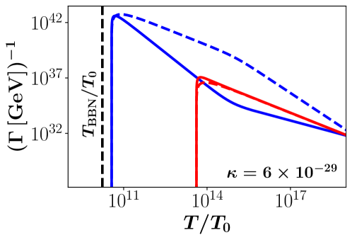
Figure 9: Evolution of $\Gamma^{-1}$ in terms of the temperature. Solid lines represent $\Gamma_{a}$ and the dashed lines $\Gamma_{b}$. In blue appears the radiation-matter case (Sec. IV.A) while the radiation-radiation (Sec.IV.B) is shown in red. It can be observed that for the same value of $\kappa$ the decay of radiation from $b$ to $a$ is faster than the case of matter.

Previous effect suggests that the present model can be understood as different type of non standard cosmology and it also suggests to include dark matter in one of the patches. This analysis will be presented in forthcoming works.

VI Acknowledgements

This work was supported by Dicyt-USACH grants USA1956-Dicyt (CM) and Dicyt-041931MF (FM).

References

- Falomir et al. (2017) H. Falomir, J. Gamboa, F. Méndez, and P. Gondolo, Phys. Rev. D 96, 083534 (2017).
- Weinberg (2008) S. Weinberg, Cosmology (Oxford University Press, New York, 2008).
- Kolb and Turner (1990) E. W. Kolb and M. S. Turner, The Early Universe, Vol. 69 (CRC Press, 1990).
- Zwicky (1933) F. Zwicky, Helv. Phys. Acta 6, 110 (1933).
- Freeman (1970) K. C. Freeman, Astrophys. J. 160, 811 (1970).
- Bertone and Hooper (2018) G. Bertone and D. Hooper, Rev. Mod. Phys. 90, 045002 (2018), arXiv:1605.04909 [astro-ph.CO] .
- Salucci (2018) P. Salucci, Found Phys. 48, 1517 (2018), arXiv:1807.08541 [astro-ph.CO] .
- Riess et al. (1998) A. G. Riess, A. V. Filippenko, P. Challis, A. Clocchiatti, A. Diercks, P. M. Garnavich, R. L. Gilliland, C. J. Hogan, S. Jha, R. P. Kirshner, and et al., The Astronomical Journal 116, 1009–1038 (1998).
- Perlmutter et al. (1999) S. Perlmutter, G. Aldering, G. Goldhaber, R. A. Knop, P. Nugent, P. G. Castro, S. Deustua, S. Fabbro, A. Goobar, D. E. Groom, and et al., The Astrophysical Journal 517, 565–586 (1999).
- Zyla et al. (2020) P. Zyla et al. (Particle Data Group), PTEP 2020, 083C01 (2020).
- Vilenkin (1985) A. Vilenkin, Physics Report 121, 263 (1985).
- Sikivie (1982) P. Sikivie, Phys. Rev. Lett. 48, 1156 (1982).
- Lukas et al. (1998) A. Lukas, B. A. Ovrut, K. S. Stelle, and D. Waldram, Phys. Rev. D 59, 086001 (1998), arXiv:arXiv:hep-th/9803235 [hep-th] .
- Flanagan et al. (2000) E. Flanagan, S.-H. Tye, and I. Wasserman, Phys. Rev. D 62, 024011 (2000), arXiv:hep-ph/9909373 [hep-ph] .
- Peebles and Vilenkin (1999) P. Peebles and A. Vilenkin, Phys. Rev. D 59, 063505 (1999), arXiv:hep-ph/9811375 [hep-ph] .
- Linde (1990) A. D. Linde, Particle physics and inflationary cosmology, Vol. 5 (Harwood Academic Publishers, 1990) arXiv:hep-th/0503203 .
- Falomir et al. (2018) H. Falomir, J. Gamboa, P. Gondolo, and F. Méndez, Phys. Lett. B 785, 399 (2018), arXiv:1801.07575 [hep-th] .
- Falomir et al. (2020) H. Falomir, J. Gamboa, and F. Mendez, Symmetry 12, 435 (2020).
- Scherrer and Turner (1985) R. J. Scherrer and M. S. Turner, Phys. Rev. D 31, 681 (1985).
- Hamdan and Unwin (1996) S. Hamdan and J. Unwin, Modern Physics Letter A 33, 1332 (1996), arXiv:1710.03758 [hep-ph] .
- Giudice et al. (2001) G. F. Giudice, E. W. Kolb, and A. Riotto, Phys. Rev. D 64, 023508 (2001), arXiv:hep-ph/0005123 [hep-ph] .
- Gelmini and Gondolo (2006) G. Gelmini and P. Gondolo, Phys. Rev. D 74, 023510 (2006), arXiv:hep-ph/0602230 [hep-ph] .
- Maldonado and Unwin (2019) C. Maldonado and J. Unwin, JCAP 06, 37 (2019), arXiv:1902.10746 [hep-ph] .
- Arias et al. (2019) P. Arias, N. Bernal, A. Herrera, and C. Maldonado, JCAP 10, 47 (2019), arXiv:1906.04183 [hep-ph] .
- Bernal et al. (2019) N. Bernal, F. Elahi, C. Maldonado, and J. Unwin, JCAP 11, 26 (2019), arXiv:1909.07992 [hep-ph] .
- Visinelli (2018) L. Visinelli, Symmetry 10, 11 (2018), arXiv:1710.11006 [astro-ph.CO] .
- Chung et al. (1999) D. J. H. Chung, E. W. Kolb, and A. Riotto, Phys. Rev. D 60, 063504 (1999), arXiv:hep-ph/9809453 [hep-ph] .
- Kolb et al. (2003) E. W. Kolb, A. Notari, and A. Riotto, Phys. Rev. D 68, 123505 (2003), arXiv:hep-ph/0307241 [hep-ph] .
- Kawasaki et al. (2000) M. Kawasaki, K. Kohri, and N. Sugiyama, Phys. Rev. D 62, 023506 (2000), arXiv:astro-ph/0002127 [astro-ph] .
- Hannestad (2004) S. Hannestad, Phys. Rev. D 70, 043506 (2004), arXiv:astro-ph/0403291 [astro-ph] .
- Bernal et al. (2020) N. Bernal, A. Ghoshal, F. Hajkarimc, and G. Lambiase, JCAP 11, 051 (2020), arXiv:arXiv:2008.04959 [gr-qc] .
- Rasouli et al. (2019) S. Rasouli, J. Marto, and P. Moniz, Physics of the Dark Universe 24, 100269 (2019).
- Linde (2017) A. Linde, Rept. Prog. Phys. 80, 022001 (2017), arXiv:1512.01203 [hep-th] .