Explicit formulas for Killing magnetic curves in Heisenberg group

Abstract

In this paper, We present the geometry three dimensional Heisenberg group $(\mathbb{H}_{3},g)$ and its geodesics curves. After, we study the Killing magnetic curves and some geodesic Killing magnetic curves with its explicit formulas for such curves.

Key words: Heisenberg group; geodesic Killing magnetic curves; Killing vector fields; Killing magnetic curves.

MSC: 53A04, 53C25

1 Introduction

In physics, particularly in electromagnetism, the trajectory of charged particles moving under the action of a magnetic fields makes an important research topic. In geometry, this trajectory in any manifold is known as a magnetic curve.

On a Riemannian manifold, the magnetic curve $\gamma$ is modeled as a solution of two order differential equation $\nabla_{\gamma^{\prime}}\gamma^{\prime}=\varphi\left(\gamma^{\prime}\right)$ known as Lorentz equation, where $\varphi$ is $(1,1)$-tensor field that present the Lorentz force associated to the magnetic fields $F$. The magnetic curve generalise the geodesic curves in following way: When the particles move under the absence of the magnetic fields so freely only under the influence of gravity (i.e. $\varphi\equiv 0$), the Lorentz equation is exactly the geodesic equation $\nabla_{\gamma^{\prime}}\gamma^{\prime}=0.$

The magnetic curve was studied intensively in different kind of manifolds in Riemannian, Lorentzian and generally in pseudo-Riemannian concept. (See [1], [6], [7], [18])

Furthermore, if the magnetic fields $F$ corresponds to a killing vector, then the trajectory of particles moving under the action of $F$ is called Killing magnetic curve.

Interesting results on Killing magnetic curves are given in Euclidian 3-space ([9]), Minkowski 3-space ([8]), $\mathbb{S}^{2}\times\mathbb{R}$ ([17]), $SL(2,\mathbb{R})$ ([10]), Sol Space ([12]), warped product manifold ([15]), almost paracontact manifold ([5]), Almost Cosymplectic Sol Space ([11]) and in Walker manifolds ([2]).

The framework of the paper is to study the Killing magnetic curves in $3$-dimensional Heisenberg group.

The contents of this study is the following: we present in the second section a general notions and definitions of killing magnetic curves.

The section $3$ is devoted to the geometry of Heisenberg group and its contact structure.

Finally in the section $4$, we classifies fourth kind of Killing magnetic curves, we give its explicit parametric formulas at each kind in different subsections and we close it with figures presented in Euclidian space.

2 Preliminaries

On Riemannian manifold $(M,g),$ the magnetic curves is a trajectories of the charged particles moving under the action of the magnetic fields $F$ which can be represented by a closed $2$-form

$$F(X,Y)=g(\varphi\left(X\right),Y)$$ (1)

where $X,Y$ are vector fields on $(M,g)$ and $\varphi$ is skew-symmetric $(1,1)$-tensor field. that present the Lorentz force associated to $F$. For a regular curve $\gamma:I\subset\mathbb{R}\rightarrow(M,g)$, $\gamma$ is called magnetic curve if

$$\nabla_{\mathbf{t}}\mathbf{t=}\varphi\left(\mathbf{t}\right)$$ (2)

known as the Lorentz equation, where $\nabla$ is the Levi-Civita connection associated to $g\$and $\mathbf{t}=\gamma^{\prime}$ is the speed vector of $\gamma.$ The magnetic curve generalise the notion of geodesic curve under arc-length parametrization.

From the property of magnetic curve $\gamma$

$$\frac{d}{dt}g(\gamma^{\prime},\gamma^{\prime})=0$$

$\gamma$ has a constant speed vector. In particular, if $\gamma$ is parameterized by the arc length, then $\gamma$ is called normal magnetic curve.

We call $K$ a Killing vector field on $M$ if it satisfy the Killing equation

$$g(\nabla_{X}K,Y)+g(\nabla_{Y}K,X)=0$$

for every vector fields $X,Y$ on $M$.

We define on M the cross product of two vector fields $X,Y$ on $M$ as

$$g(X\times Y,Z)=dvg(X,Y,Z)$$ (3)

for all vector fields $Z$ on $M$ and $dvg$ denotes the volume form on $M.$

Let $F_{K}=\emph{i}_{K}dvg$ be the Killing magnetic field corresponding to the Killing vector field $K$ on $M$, where i is inner product. Then, the $(1,1)$-tensor fields corresponding to the Lorentz force of $F_{K}$ is

$$\gamma(X)=K\times X.$$ (4)

Then, we can rewrite the Lorentz equation Eq.(2) as

$$\nabla_{\mathbf{t}}\mathbf{t=}K\times\mathbf{t}$$ (5)

and the it solution is called Killing magnetic curves corresponding to the killing vector fields $K.$

In the sequel, to simplify, we call this curve a $K$-magnetic curve.

3 Geometry structure of $\mathbb{H}_{3}$

The Heisenberg group $\mathbb{H}_{3}$ is a quasi-abelian Lie group diffeomorphic to $\mathbb{R}^{3}$ and it has the standard representation in $GL(3,\mathbb{R})$ as

$$\mathbb{H}_{3}=\left\{\left(\begin{array}[]{ccc}0&x&z\\ 0&0&y\\ 0&0&0\end{array}\right)\mid\left(x,y,z\right)\in\mathbb{R}^{3}\right\}$$

endowed with the multiplication

$$(x_{1},y_{1},z_{1})(x_{2},y_{2},z_{2})=(x_{1}+x_{2},y_{1}+y_{2},z_{1}+z_{2}-x_{1}y_{2}).$$

The invariant Riemannian metric with respect to the left-translations corresponding to that multiplication is denoted by

$$g=\frac{1}{\lambda^{2}}dx^{2}+dy^{2}+(xdy+dz)^{2}.$$ (6)

where $\lambda$ is a strictly positive real number. All left-invariant Riemannian metric on the $\mathbb{H}_{3}$ is isometric to the metric $g$.

The Levi-Civita connection $\nabla$ of the metric $g$ with respect to the left-invariant orthonormal basis

$$e_{1}=\partial y-x\partial z,\ \ e_{2}=\lambda\partial x,\ \ e_{3}=\partial z,$$ (7)

with dual basis

$$\omega^{1}=dy;\ \ \omega^{2}=\frac{1}{\lambda}dx;\ \ \omega^{3}=xdy+dz.$$

are given by

$$\left\{\begin{array}[]{l}\nabla_{e_{1}}e_{1}=0\\ \nabla_{e_{1}}e_{2}=\frac{\lambda}{2}e_{3}\\ \nabla_{e_{1}}e_{3}=-\frac{\lambda}{2}e_{2}\end{array}\begin{array}[]{l}\nabla_{e_{2}}e_{1}=-\frac{\lambda}{2}e_{3}\\ \nabla_{e_{2}}e_{2}=0\\ \nabla_{e_{2}}e_{3}=\frac{\lambda}{2}e_{1}\end{array}\begin{array}[]{l}\nabla_{e_{3}}e_{1}=-\frac{\lambda}{2}e_{2}\\ \nabla_{e_{3}}e_{2}=\frac{\lambda}{2}e_{1}\\ \nabla_{e_{3}}e_{3}=0\end{array}\right.$$ (8)

The Lie bracket of the base $\left(e_{i}\right)_{i=\overline{1,3}}$ are given by the following identities

$$[e_{1},e_{2}]=\lambda e_{3};\ \ \ [e_{1},e_{3}]=[e_{2},e_{3}]=0$$ (9)

The Lie algebra of Killing vector field of $(\mathbb{H}_{3},g)$ is generated by the following killing vectors

$$\mathbf{K}_{1} = \partial z,\ \ \mathbf{K}_{2}=\partial y,\ \ \mathbf{K}_{3}=\partial x-y\partial z\ and$$

$$\mathbf{K}_{4} = \lambda^{2}y\partial x-x\partial y-\frac{1}{2}(\lambda^{2}y^{2}-x^{2})\partial z,$$

and using the Eq.(7), we can rewrite the killing vectors in the base $\left(e_{i}\right)_{i=\overline{1,3}}$ as

$$\mathbf{K}_{1} = e_{3},\ \ \mathbf{K}_{2}=e_{1}+xe_{3},\ \ \ \ \mathbf{K}_{3}=\frac{1}{\lambda}e_{2}-ye_{3}\ and$$ (10)

$$\ \mathbf{K}_{4} = -xe_{1}+\lambda ye_{2}-\frac{1}{2}(\lambda^{2}y^{2}-3x^{2})e_{3}.$$

for more detail see ([3]).

On the other hand, for the contact form

$$\eta=xdy+dz=\omega^{3}$$ (11)

and the $(1,1)$-tensor $\varphi$ given in base $\left(e_{i}\right)_{i=\overline{1,3}}$ by

$$\varphi\left(e_{1}\right)=e_{2};\ \varphi\left(e_{2}\right)=-e_{1}\ and\ \varphi\left(e_{3}\right)=0$$ (12)

we have

$$\eta\left(e_{3}\right) = 1;\ \varphi^{2}\left(X\right)=-X+\eta\left(X\right)e_{3}\ and$$

$$g(\varphi\left(X\right),\varphi\left(Y\right)) = g(X,Y)+\eta(X)\eta(Y)$$

for any $X,Y\in\chi(\mathbb{H}_{3})$ and $\xi=e_{3}$, the Heisenberg group $(\mathbb{H}_{3},\varphi,\xi,\eta,g)$ is an almost contact manifold. Moreover, we have

$$d\eta(X,Y)=g(X,\varphi\left(Y\right))$$ (13)

then $(\mathbb{H}_{3},\varphi,\xi,\eta,g)$ is a contact manifold and the fundamental $2$-form $d\eta$ is closed and hence it defines a magnetic field. For more detail see ([13], [14], [4], [16]).

4 Killing magnetic curves in $\mathbb{H}_{3}$

In this section, we have used two computer softwares (Wolfram Mathematica and Scientific Workplace) to solve some differential systems and for curve figures.

Let $\gamma(t)=(x(t),y(t),z(t)):I\subset\mathbb{R\rightarrow}\left(\mathbb{H}_{3},g\right)$ be a regular curve. Its speed curve is

$$\gamma^{\prime}(t)=\mathbf{t}=(x^{\prime}(t),y^{\prime}(t),z^{\prime}(t))$$ (14)

from the Eq.(7), the speed vector $\mathbf{t}$ is expressed in the base $\left(e_{i}\right)_{i=\overline{1,3}}$ as

$$\mathbf{t}=y^{\prime}e_{1}+\frac{x^{\prime}}{\lambda}e_{2}+\left(z^{\prime}+xy^{\prime}\right)e_{3}$$ (15)

Using the connection formulas given in the Eq.(8), the covariant derivative of the speed vector $\mathbf{t}$ is

$$\nabla_{\mathbf{t}}\mathbf{t=}\left(y^{\prime\prime}+x^{\prime}\left(z^{\prime}+xy^{\prime}\right)\right)e_{1}+\left(\frac{x^{\prime\prime}}{\lambda}+\lambda y^{\prime}\left(z^{\prime}+xy^{\prime}\right)\right)e_{2}+\left(z^{\prime}+xy^{\prime}\right)^{\prime}e_{3}$$ (16)

We know that the equation of geodesics is a particular case of the Lorentz equation given in Eq.(2) when the Lorentz force vanishes, the geodesics is a particular magnetic trajectories. A simple computation of the geodesic equation $\nabla_{\mathbf{t}}\mathbf{t}=0,$ give a differential equations system

$$S_{G}:\left\{\begin{array}[]{l}y^{\prime\prime}+x^{\prime}\left(z^{\prime}+xy^{\prime}\right)=0\\ x^{\prime\prime}+\lambda^{2}y^{\prime}\left(z^{\prime}+xy^{\prime}\right)=0\\ \left(z^{\prime}+xy^{\prime}\right)^{\prime}=0\end{array}\right.$$

where its general solutions are explicit formulas of geodesic curves $\gamma_{G}$ in $(\mathbb{H}_{3},g)$ given by the following proposition.

Proposition 1

The parametric equations of the geodesic curves $\gamma_{G}$ in $(\mathbb{H}_{3},g)$ is given by

$$\begin{array}[]{l}i.\ \gamma_{G}(t)=\left\{\begin{array}[]{l}x\left(t\right)=c_{1}t+c_{2}\\ y\left(t\right)=c_{3}t+c_{4}\\ z(t)=\frac{c_{1}c_{3}}{2}t^{2}+c_{2}c_{3}t+c_{5}\end{array}\right.\text{ or}\\ ii.\ \gamma_{G}(t)=\left\{\begin{array}[]{l}x\left(t\right)=-\frac{c_{1}}{c}e^{c\lambda t}-\frac{c_{2}}{c}e^{-c\lambda t}+c_{3}\\ y\left(t\right)=\frac{c_{1}}{c\lambda}e^{c\lambda t}-\frac{c_{2}}{c\lambda}e^{-c\lambda t}+c_{4}\\ z(t)=\frac{2c_{1}c_{2}+c^{2}}{c}t-\frac{c_{3}}{\lambda c}\left(c_{1}e^{ct\lambda}-c_{2}e^{-ct\lambda}\right)+\left(\frac{c_{1}^{2}-c_{2}^{2}}{2c^{2}\lambda}\right)e^{-2c\lambda t}\end{array}\right.\end{array}$$ (17)

where $c_{\overline{1,4}}$ are a real constants.

4.1 $\mathbf{K}_{1}$- magnetic curves

We consider $\mathbf{K}_{1}$-magnetic curves which correspond to the Killing vector field $\mathbf{K}_{1}=e_{3}=\partial z.$

Firstly, we have the product vector

$$\mathbf{K}_{1}\times\mathbf{t}=-\frac{x^{\prime}}{\lambda}e_{1}+y^{\prime}e_{2}$$ (18)

We can also obtain the Eq.(18) in the following way.
Because $\mathbf{K}_{1}=\xi$ given from the almost contact structure $(\mathbb{H}_{3},\varphi,\xi,\eta,g)$, the magnetic fields $F_{\mathbf{K}_{1}}$ corresponding to $\mathbf{K}_{1}$ is exactly the magnetic fields $F$ associated to Lorentz force which presented  by the skew-symmetric $(1,1)$-tensor $\varphi$ given by the Eq.(12).

Thus, we find the right-hand side of the relation given in Eq.(18)

$$\varphi\left(\mathbf{t}\right) = \varphi\left(y^{\prime}e_{1}+\frac{x^{\prime}}{\lambda}e_{2}+\left(z^{\prime}+xy^{\prime}\right)e_{3}\right)$$

$$= y^{\prime}e_{2}-\frac{x^{\prime}}{\lambda}e_{1}=\mathbf{K}_{1}\times\mathbf{t}$$

Now, to find the explicit formulas of $\mathbf{K}_{1}$-magnetic curves, we must solve the differential equations system denoted by $(S_{1})$, given from the Eqs.(16, 18) and Lorentz equation

$$\nabla_{\mathbf{t}}\mathbf{t}=\mathbf{K}_{1}\times\mathbf{t}$$

The system $(S_{1})$ is

$$S_{1}:\left\{\begin{array}[]{l}y^{\prime\prime}+x^{\prime}\left(\left(z^{\prime}+xy^{\prime}\right)+\frac{1}{\lambda}\right)=0\\ x^{\prime\prime}+y^{\prime}\left(\lambda^{2}\left(z^{\prime}+xy^{\prime}\right)-\lambda\right)=0\\ \left(z^{\prime}+xy^{\prime}\right)^{\prime}=0\end{array}\right.$$

After integrating the third equation $\left(S_{1_{3}}\right)$ and replaced them in the equations $\left(S_{1_{1,2}}\right)$, the system $(S)$ turns to

$$S_{1}:\left\{\begin{array}[]{l}y^{\prime\prime}+x^{\prime}\left(c+\frac{1}{\lambda}\right)=0\\ x^{\prime\prime}+y^{\prime}\lambda\left(\lambda c-1\right)=0\\ z^{\prime}+xy^{\prime}=c\ \ (constant)\end{array}\right.$$

the general solution of the equations $(S_{1_{1,2}})$ is

$$\left\{\begin{array}[]{c}x\left(t\right)=\frac{\lambda}{\lambda c+1}\left(c_{1}e^{\sqrt{\lambda^{2}c^{2}-1}t}+c_{2}e^{-\sqrt{\lambda^{2}c^{2}-1}t}\right)+c_{3}\\ y\left(t\right)=\frac{1}{\sqrt{\lambda^{2}c^{2}-1}}\left(c_{1}e^{\sqrt{\lambda^{2}c^{2}-1}t}-c_{2}e^{-\sqrt{\lambda^{2}c^{2}-1}t}\right)+c_{4}\end{array}\right.$$ (19)

where $c_{\overline{1,4}}$ are a real constants, $\left|\lambda c\right|>1$ (if $\left|\lambda c\right|<1$ the system don’t admit a real solutions) and $\lambda c\neq\pm 1$ (we studied these cases $\lambda c=\pm 1$ later).

Substituting the Eq.(19) in the equation $(S_{1_{3}})$ and by an integration with respect to $t$, we have

$$z(t)=\left(c+\frac{2\lambda}{\lambda c+1}c_{1}c_{2}\right)t+\frac{1}{\sqrt{\lambda^{2}c^{2}-1}}\left(\begin{array}[]{c}c_{1}c_{3}e^{-t\sqrt{\lambda^{2}c^{2}-1}}-c_{2}c_{3}e^{t\sqrt{\lambda^{2}c^{2}-1}}+\\ \frac{\lambda}{2\left(\lambda c+1\right)}\left(c_{1}^{2}e^{-2t\sqrt{\lambda^{2}c^{2}-1}}-c_{2}^{2}e^{2t\sqrt{\lambda^{2}c^{2}-1}}\right)\end{array}\right)+c_{5}$$

where $c_{5}$ is real constant.

If $c=\dfrac{1}{\lambda},$ we rewrite the system $(S_{1})$ as

$$S_{1}:\left\{\begin{array}[]{l}y^{\prime\prime}+x^{\prime}\frac{2}{\lambda}=0\\ x^{\prime\prime}=0\\ z^{\prime}+xy^{\prime}=\dfrac{1}{\lambda}\end{array}\right.$$

Its general solution is

$$\left\{\begin{array}[]{l}x\left(t\right)=c_{1}t+c_{2},\\ y\left(t\right)=\frac{-c_{1}}{\lambda}t^{2}+c_{3}t+c_{4}\\ z\left(t\right)=\frac{2c_{1}^{2}}{3\lambda}t^{3}+c_{1}\left(\frac{c_{2}}{\lambda}-\frac{c_{3}}{2}\right)t^{2}+\left(\frac{1}{\lambda}-c_{2}c_{3}\right)t+c_{5}\end{array}\right.$$

where $c_{\overline{1,5}}$ are a real constants.

If $c=\dfrac{-1}{\lambda},$ the system $(S_{1})$ is

$$S_{1}:\left\{\begin{array}[]{l}y^{\prime\prime}=0\\ x^{\prime\prime}-2y^{\prime}\lambda=0\\ z^{\prime}+xy^{\prime}=\dfrac{-1}{\lambda}\end{array}\right.$$

with a general solution

$$\left\{\begin{array}[]{l}x\left(t\right)=c_{1}\lambda t^{2}+c_{2}t+c_{3},\\ y\left(t\right)=c_{1}t+c_{4}\\ z\left(t\right)=\frac{c_{1}c_{2}}{2}t^{2}+\left(\dfrac{-1}{\lambda}+c_{3}c_{1}-\frac{c_{1}^{2}}{3}\lambda\right)t+c_{5}\end{array}\right.$$

Now, we can present the following theorem.

Theorem 2

The explicit formulae of all $\mathbf{K}_{1}$-magnetic curves in $(\mathbb{H}_{3},g)$ are the space curves given by parametric equations:
1.
$\gamma(t)=\left(\begin{array}[]{l}x\left(t\right)=c_{1}t+c_{2},\\ y\left(t\right)=\frac{-c_{1}}{\lambda}t^{2}+c_{3}t+c_{4}\\ z\left(t\right)=\frac{2c_{1}^{2}}{3\lambda}t^{3}+c_{1}\left(\frac{c_{2}}{\lambda}-\frac{c_{3}}{2}\right)t^{2}+\left(\frac{1}{\lambda}-c_{2}c_{3}\right)t+c_{5}\end{array}\right)$ or
2.
$\gamma(t)=\left(\begin{array}[]{l}x\left(t\right)=c_{1}\lambda t^{2}+c_{2}t+c_{3},\\ y\left(t\right)=c_{1}t+c_{4}\\ z\left(t\right)=\frac{c_{1}c_{2}}{2}t^{2}+\left(\tfrac{-1}{\lambda}+c_{3}c_{1}-\frac{c_{1}^{2}}{3}\lambda\right)t+c_{5}\end{array}\right)$ or
3.
$\gamma(t)=\left(\begin{array}[]{l}x\left(t\right)=\frac{\lambda}{\lambda c+1}\left(c_{1}e^{\sqrt{\lambda^{2}c^{2}-1}t}+c_{2}e^{-\sqrt{\lambda^{2}c^{2}-1}t}\right)+c_{3}\\ y\left(t\right)=\frac{1}{\sqrt{\lambda^{2}c^{2}-1}}\left(c_{1}e^{\sqrt{\lambda^{2}c^{2}-1}t}-c_{2}e^{-\sqrt{\lambda^{2}c^{2}-1}t}\right)+c_{4}\\ z\left(t\right)=\left(c+\frac{2\lambda c_{1}c_{2}}{\lambda c+1}\right)t+\frac{1}{\sqrt{\lambda^{2}c^{2}-1}}\left(\begin{array}[]{c}c_{3}\left(c_{1}e^{-t\sqrt{\lambda^{2}c^{2}-1}}-c_{2}e^{t\sqrt{\lambda^{2}c^{2}-1}}\right)+\\ \frac{\lambda}{2\left(\lambda c+1\right)}\left(c_{1}^{2}e^{-2t\sqrt{\lambda^{2}c^{2}-1}}-c_{2}^{2}e^{2t\sqrt{\lambda^{2}c^{2}-1}}\right)\end{array}\right)+c_{5}\end{array}\right)$
where in (3), $\left|\lambda c\right|>1$ and $c,c_{\overline{1,5}}$ are a real constants.

Corollary 3

The curve presented in assertion (1) of the Theorem (2) for $c_{1}=0$ and $\lambda=\frac{1}{2c_{2}c_{3}}$ is a geodesic $\mathbf{K}_{1}$-magnetic curve in $(\mathbb{H}_{3},g).$

Proof. It’s a direct consequence from the geodesic curve formulas in Eq.(17) an the Theorem (2).    

We present in $(\mathbb{R}_{3},g_{euc})$ some examples of $\mathbf{K}_{1}$-magnetic curve in $(\mathbb{H}_{3},g)$ in following figures drawing in $(\mathbb{R}_{3},g_{euc})$.
For $c_{1,2.3}=1;\ \ c_{4,5}=0$ and$\ \lambda=1$, the figure 1 at left side, present the $\mathbf{K}_{1}$-magnetic curve for the first assertion in $(\mathbb{H}_{3},g)$.

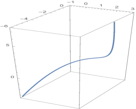
Figure 1: $\mathbf{K}_{1}$-magnetic curve

For $c_{1,2}=\lambda=1\$and$\ c_{3,4,5}=0,$ the figure 1 at right side, present the $\mathbf{K}_{1}$-magnetic curve for the assertion (2) in $(\mathbb{H}_{3},g)$.

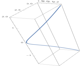
Figure 2: $\mathbf{K}_{1}$-magnetic curve

For $c_{1,2,3}=1;\ \ c_{4,5}=0$ and$\ \lambda=1;\ c=\sqrt{2}$ (i.e. $\left|\lambda c\right|>1$), the figure 2 present the $\mathbf{K}_{1}$-magnetic curve for the assertion (3) in $(\mathbb{H}_{3},g)$.

4.2 $\mathbf{K}_{2}$-magnetic curves

Similarly, as in subsection (4.1), we have

$$\mathbf{K}_{2}\times\mathbf{t}=-\frac{x^{\prime}x}{\lambda}e_{1}+\left(xy^{\prime}-\left(z^{\prime}+xy^{\prime}\right)\right)e_{2}+\frac{x^{\prime}}{\lambda}e_{3}$$ (20)

We can find a same formula as the Eq.(20) using the Eqs.(3, 4 and 11) to determine the magnetic fields $F_{\mathbf{K}_{2}}$and associated skew-symmetric $(1,1)$-tensor $\varphi.$

The $\mathbf{K}_{2}$-magnetic curves are the solution of the differential equations system

$$S_{2}:\left\{\begin{array}[]{l}x^{\prime}\left(z^{\prime}+xy^{\prime}\right)=-y^{\prime\prime}-\frac{xx^{\prime}}{\lambda}\\ \left(\lambda y^{\prime}+1\right)\left(z^{\prime}+xy^{\prime}\right)=xy^{\prime}-\frac{x^{\prime\prime}}{\lambda}\\ \left(z^{\prime}+xy^{\prime}\right)^{\prime}=\frac{x^{\prime}}{\lambda}\end{array}\right.$$

given from the Eqs.(16, 20) and Lorentz equation

$$\nabla_{\mathbf{t}}\mathbf{t}=\mathbf{K}_{2}\times\mathbf{t}$$

after integrating the equation $\left(S_{2_{3}}\right),$ we have

$$z^{\prime}+xy^{\prime}=\frac{x}{\lambda}+c\text{ }$$ (21)

here $c$ is a arbitrary real constant. Substituting the last equation in the equations $\left(S_{2_{2,3}}\right),$ we get the system

$$\overline{S}_{2}:\left\{\begin{array}[]{l}x^{\prime}\left(\frac{2x}{\lambda}+c\right)=-y^{\prime\prime}\\ \left(\lambda y^{\prime}+1\right)\left(\frac{x}{\lambda}+c\right)=xy^{\prime}-\frac{x^{\prime\prime}}{\lambda}\end{array}\right.$$

and

$$\overline{S}_{2}:\left\{\begin{array}[]{l}y^{\prime}=-\frac{x^{2}}{\lambda}-xc\\ x^{\prime\prime}-cx^{2}\lambda+x\left(1-c^{2}\lambda^{2}\right)+c\lambda=0.\end{array}\right.$$

it is very difficult to find exact solutions of the system ($\overline{S}_{2}$) for every constant $c$. However, without loss of generality, we can assume that $c=0,$ the solution can be given as

$$\left\{\begin{array}[]{l}x(t)=c_{1}\cos t-c_{2}\sin t\\ y(t)=\frac{1}{2\lambda}c_{1}c_{2}\cos 2t+\frac{1}{4\lambda}\left(c_{1}^{2}-c_{2}^{2}\right)\sin 2t+\frac{1}{2\lambda}\left(c_{1}^{2}+c_{2}^{2}\right)t\end{array}\right.$$

Substituting the solutions $x(t)$ and $y(t)$ in Eq.(21) and by an integration, we have the following solution

$$z(t)=\frac{1}{\lambda}\left(\begin{array}[]{c}\frac{1}{4}c_{2}\left(c_{1}^{2}-\frac{1}{3}c_{2}^{2}\right)\cos 3t+\frac{1}{4}c_{1}\left(\frac{1}{3}c_{1}^{2}-c_{2}^{2}\right)\sin 3t\\ +\left(1+\frac{3}{4}\left(c_{2}^{2}+c_{1}^{2}\right)\right)\left(c_{2}\cos t+c_{1}\sin t\right)\end{array}\right)$$

Then we have the following theorem:

Theorem 4

The space curves given by parametric equations

$$\gamma(t)=\left\{\begin{array}[]{l}x(t)=c_{1}\cos t-c_{2}\sin t\\ y(t)=\frac{1}{2\lambda}c_{1}c_{2}\cos 2t+\frac{1}{4\lambda}\left(c_{1}^{2}-c_{2}^{2}\right)\sin 2t+\frac{1}{2\lambda}\left(c_{1}^{2}+c_{2}^{2}\right)t\\ z(t)=\frac{1}{\lambda}\left(\begin{array}[]{c}\frac{1}{4}c_{2}\left(c_{1}^{2}-\frac{1}{3}c_{2}^{2}\right)\cos 3t+\frac{1}{4}c_{1}\left(\frac{1}{3}c_{1}^{2}-c_{2}^{2}\right)\sin 3t\\ +\left(1+\frac{3}{4}\left(c_{2}^{2}+c_{1}^{2}\right)\right)\left(c_{2}\cos t+c_{1}\sin t\right)\end{array}\right)\end{array}\right.$$

are $\mathbf{K}_{2}$-Killing magnetic curves in $(\mathbb{H}_{3},g),$ where $c_{1},\ c_{2}$ are a real constants.

Corollary 5

There is no $\mathbf{K}_{2}$-magnetic curves od the space curves of the Theorem (4) which is a geodesic in $(\mathbb{H}_{3},g).$

In $(\mathbb{R}_{3},g_{euc}),$ we present an example of $\mathbf{K}_{2}$-magnetic curve in $(\mathbb{H}_{3},g)$ in figure $3$ with $c_{1}=2c_{2}=2$ and $\lambda=1.$

Figure 3: $\mathbf{K}_{2}$-magnetic curve in $(\mathbb{H}_{3},g)$ presented in $(\mathbb{R}_{3},g_{euc})$

4.3 $\mathbf{K}_{3}$-magnetic curves

As above in subsections 4.1 and 4.2, we have the product vector

$$\mathbf{K}_{3}\times\mathbf{t=}\frac{1}{\lambda}\left(yx^{\prime}+z^{\prime}+xy^{\prime}\right)e_{1}-yy^{\prime}e_{2}-\frac{1}{\lambda}y^{\prime}e_{3}$$

Also, we can find a same formula as the Eq.(20) using the Eqs.(3, 4 and 11) to determine the magnetic fields $F_{\mathbf{K}_{2}}$and the associated skew-symmetric $(1,1)$-tensor $\varphi.$

Using the Eqs(16, 20) and

$$\nabla_{\mathbf{t}}\mathbf{t}=\mathbf{K}_{3}\times\mathbf{t}$$

we have the differential equations system $\left(S_{3}\right)$

$$S_{3}:\left\{\begin{array}[]{c}y^{\prime\prime}+x^{\prime}\left(z^{\prime}+xy^{\prime}\right)=\frac{1}{\lambda}\left(z^{\prime}+xy^{\prime}\right)+y\frac{x^{\prime}}{\lambda}\\ \frac{x^{\prime\prime}}{\lambda}+\lambda y^{\prime}\left(z^{\prime}+xy^{\prime}\right)=-yy^{\prime}\\ \left(z^{\prime}+xy^{\prime}\right)^{\prime}=-\frac{1}{\lambda}y^{\prime}\end{array}\right.$$

The integration of the third equation $\left(S_{3_{3}}\right)$, give

$$z^{\prime}+xy^{\prime}=-\frac{1}{\lambda}y+c$$ (22)

substituting the last equation in equations $\left(S_{3_{1,2}}\right),$ we have the differential equations system

$$\overline{S}_{3}:\left\{\begin{array}[]{c}y^{\prime\prime}+2\lambda cy^{2}+y\left(\frac{1}{\lambda^{2}}-\lambda^{2}c^{2}\right)-\frac{c}{\lambda}=0\\ x^{\prime}=-\lambda^{2}cy\end{array}\right.$$

Analogously as the subsection 4.2, it is a true challenge to find exact solutions for the system ($\overline{S}_{3}$). Therefore, we try to solve’it in particular case $c=0$.

By integrating the system $\left(\overline{S}_{3}\right)$ in the case $c=0,$ we find the general solution

$$\left\{\begin{array}[]{l}x(t)=c_{1}t+c_{2}\\ y(t)=c_{3}\exp\left(\frac{\sqrt{2\lambda c_{1}-1}}{\lambda}t\right)+c_{4}\exp\left(\frac{-\sqrt{2\lambda c_{1}-1}}{\lambda}t\right)\end{array}\right.$$

Substituting the solutions $x(t)$ and $y(t)$ in the Eq.(22), we get

$$z(t)=\begin{array}[]{c}\left(\frac{-c_{3}}{\sqrt{2\lambda c_{1}-1}}-c_{3}\left(c_{2}-\lambda c_{1}\sqrt{2\lambda c_{1}-1}+c_{1}t\right)\right)\exp\left(\frac{\sqrt{2\lambda c_{1}-1}}{\lambda}t\right)\\ +\left(\frac{c_{4}}{\sqrt{2\lambda c_{1}-1}}-c_{4}\left(c_{2}+\lambda c_{1}\sqrt{2\lambda c_{1}-1}+c_{1}t\right)\right)\exp\left(-\frac{\sqrt{2\lambda c_{1}-1}}{\lambda}t\right)\end{array}$$

where $c_{\overline{1,4}}$ are an arbitrary real constants.

Finally, we can present the following theorem.

Theorem 6

The space curves given by parametric equations

$$\gamma(t)=\left(\begin{array}[]{l}x(t)=c_{1}t+c_{2}\\ y(t)=c_{3}\exp\left(\frac{\sqrt{2\lambda c_{1}-1}}{\lambda}t\right)+c_{4}\exp\left(\frac{-\sqrt{2\lambda c_{1}-1}}{\lambda}t\right)\\ z(t)=\begin{array}[]{c}\left(\frac{-c_{3}}{\sqrt{2\lambda c_{1}-1}}-c_{3}\left(c_{2}-\lambda c_{1}\sqrt{2\lambda c_{1}-1}+c_{1}t\right)\right)\exp\left(\frac{\sqrt{2\lambda c_{1}-1}}{\lambda}t\right)\\ +\left(\frac{c_{4}}{\sqrt{2\lambda c_{1}-1}}-c_{4}\left(c_{2}+\lambda c_{1}\sqrt{2\lambda c_{1}-1}+c_{1}t\right)\right)\exp\left(-\frac{\sqrt{2\lambda c_{1}-1}}{\lambda}t\right)\end{array}\end{array}\right)$$

are $\mathbf{K}_{3}$-magnetic curves in $(\mathbb{H}_{3},g),$ where $c_{\overline{1,4}}$ are a real constants.

Corollary 7

There is no $\mathbf{K}_{3}$-magnetic curves of the space curves of the Theorem (6) which is a geodesic in $(\mathbb{H}_{3},g).$

The following figure present in $(\mathbb{R}_{3},g_{euc})$ an example of $\mathbf{K}_{3}$-magnetic curve in $(\mathbb{H}_{3},g)$ with $c_{\overline{1,4}}=1$ and $\lambda=1.$

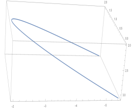
Figure 4: $\mathbf{K}_{3}$-magnetic curve in $(\mathbb{H}_{3},g)$ presented in $(\mathbb{R}_{3},g_{euc})$

4.4 $\mathbf{K}_{4}$-magnetic curves

Finally, as subsections 4.1, 4.2 and 4.3, we consider $\mathbf{K}_{4}$-magnetic curves which correspond to the Killing vector field $\mathbf{K}_{4}.$

Firstly, we have the product vector

$$\mathbf{K}_{4}\times\mathbf{t} = -\frac{1}{2\lambda}\left(3x^{2}x^{\prime}-y^{2}x^{\prime}\lambda^{2}-2y\lambda^{2}\left(z^{\prime}+xy^{\prime}\right)\right)e_{1}$$

$$-\frac{1}{2}\left(-3x^{2}y^{\prime}+y^{2}y^{\prime}\lambda^{2}-2x\left(z^{\prime}+xy^{\prime}\right)\right)e_{2}-\frac{1}{\lambda}\left(xx^{\prime}+yy^{\prime}\lambda^{2}\right)e_{3}$$

The same formula can be found as the Eq.(4.4), using the Eqs.(3, 4 and 11) to determine the magnetic fields $F_{\mathbf{K}_{4}}$and the associated skew-symmetric $(1,1)$-tensor $\varphi.$

Using the Eqs(16, 4.4) and Lorentz equation formula

$$\nabla_{\mathbf{t}}\mathbf{t}=\mathbf{K}_{4}\times\mathbf{t}$$

we have the differential equations system $\left(S_{4}\right)$

$$S_{4}:\left\{\begin{array}[]{l}y^{\prime\prime}+x^{\prime}\left(z^{\prime}+xy^{\prime}\right)=\frac{3}{2\lambda}x^{2}x^{\prime}-\frac{\lambda}{2}y^{2}x^{\prime}-\lambda y\left(z^{\prime}+xy^{\prime}\right)\\ x^{\prime\prime}+\lambda^{2}y^{\prime}\left(z^{\prime}+xy^{\prime}\right)=\frac{3\lambda}{2}x^{2}y^{\prime}-\frac{\lambda^{3}}{2}y^{2}y^{\prime}+\lambda x\left(z^{\prime}+xy^{\prime}\right)\\ \left(z^{\prime}+xy^{\prime}\right)^{\prime}=-\lambda yy^{\prime}-x\frac{x^{\prime}}{\lambda}\end{array}\right.$$

the integration of the third equation $\left(S_{4_{3}}\right),$ give

$$z^{\prime}+xy^{\prime}=-\frac{x^{2}}{2\lambda}-\frac{\lambda}{2}y^{2}+c$$ (24)

Substituting the last equation in the equations $\left(S_{4_{1,2}}\right)$, we get

$$\overline{S}_{4}:\left\{\begin{array}[]{l}y^{\prime\prime}-\frac{2}{\lambda}x^{2}x^{\prime}=\frac{1}{2}y\left(y^{2}\lambda^{2}+x^{2}\right)-c\left(y\lambda+x^{\prime}\right)\\ x^{\prime\prime}-2y^{\prime}x^{2}\lambda=-\frac{1}{2}x\left(y^{2}\lambda^{2}+x^{2}\right)+c\left(x\lambda-cy^{\prime}\lambda^{2}\right)\end{array}\right.$$

It is not essay to solve the last differential equations system $\left(\overline{S}\right)$ or is not exactly solvable in general case, however we can solve’it in particular case when $c=0$ and let $x(t)=y(t)$ and taking account that $y^{2}\lambda^{2}+x^{2}\neq 0,$ then $\left(\overline{S}_{4}\right)$ terns to

$$y^{\prime\prime}-\frac{1+\lambda^{2}}{\lambda}y^{2}y^{\prime}=0$$

by integrating the last equation with respect to $y$, we have

$$y^{\prime}-\frac{1+\lambda^{2}}{3\lambda}y^{3}=c_{1}$$

where $c_{1}$ is a real constant. Without loss of generality, we can assume that $c_{1}=0,$ then the non null solution is

$$y(t)=\pm\frac{1}{\sqrt{2}\sqrt{c_{2}-\left(\frac{1+\lambda^{2}}{3\lambda}\right)t}}$$

where $c_{2}$ is a constant. From the Eq.(24), we have

$$z(t)=\frac{3}{4}\ln\left|\left(\frac{1+\lambda^{2}}{3\lambda}\right)t-c_{2}\right|\pm\frac{1}{4\left(c_{2}-\left(\frac{1+\lambda^{2}}{3\lambda}\right)t\right)}+c_{3}$$

where $c_{2},c_{3}$ are a real constants. then we have the theorem.

Theorem 8

The space curves given by parametric equations

$$\gamma(t)=\left(\begin{array}[]{l}x(t)=\frac{1}{\sqrt{2}\sqrt{c_{1}-\left(\frac{1+\lambda^{2}}{3\lambda}\right)t}}\\ y(t)=\pm\frac{1}{\sqrt{2}\sqrt{c_{1}-\left(\frac{1+\lambda^{2}}{3\lambda}\right)t}}\\ z(t)=\frac{3}{4}\ln\left|\left(\frac{1+\lambda^{2}}{3\lambda}\right)t-c_{1}\right|\pm\frac{1}{4\left(c_{1}-\left(\frac{1+\lambda^{2}}{3\lambda}\right)t\right)}+c_{2}\end{array}\right)$$

are $\mathbf{K}_{4}$-magnetic curves in $(\mathbb{H}_{3},g)$, where $c_{1},c_{2}$ are an arbitrary real constants.

Corollary 9

There is no $\mathbf{K}_{4}$-magnetic curves of the space curves of the Theorem (8) which is a geodesic in $(\mathbb{H}_{3},g).$

Finally, we present in the following figure in $(\mathbb{R}_{3},g_{euc}),$ an example of $\mathbf{K}_{4}$-magnetic curve in $(\mathbb{H}_{3},g)$ where $c_{1}=c_{2}=0$ and $\lambda=1.$

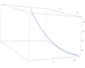
Figure 5: $\mathbf{K}_{4}$-magnetic curve in $(\mathbb{H}_{3},g)$ presented in $(\mathbb{R}_{3},g_{euc})$

References

[1] M. Barros, A. Romero: Magnetic vortices, EPL 77 (2007), 34002.
[2] C. Bejan, S. L. Drută-Romaniuc. Walker manifolds and
Killing magnetic curves, Diff. Geo. and its App. , 35 (2014), 106-116.
doi.org/10.1016/j.difgeo.2014.03.001.
[3] W. Batat, A. Zaeim. On symmetries of the Heisenberg group,
arXiv:1710.04539v1.
[4] L. Capogna, D. Danielli, S.D. Pauls, J.T. Tyson. An
introduction to the Heisenberg group and the sub-Riemannian isoperimetric
problem. (Progress in Mathematics). Birkhäuser Verlag, Basel (2007).
[5] G. Calvaruso, M. I. Munteanu, A. Perrone. Killing magnetic
curves in three-dimensional almost paracontact manifolds, J. of Math. Ana.
and App., 426(1), (2015), 423-439. doi.org/10.1016/j.jmaa.2015.01.057
[6] S. L. Drută-Romaniuc, J. Inoguchi, M. I. Munteanu and A.
I. Nistor: Magnetic curves in cosymplectic manifolds, Rep. Math. Phys. 78
(2016), 33.
[7] S. L. Drută-Romaniuc, J. Inoguchi, M. I. Munteanu, A. I.
Nistor: Magnetic curves in Sasakian manifolds, J. Nonlinear Math. Phys. 22
(2015), 428.
[8] S. L. Drută-Romaniuc, M. I. Munteanu. Killing magnetic
curves in a Minkowski 3-space, Nonlinear Analysis: Real World Appl. 14
(2013), 383.
[9] S. L. Drută-Romaniuc and M. I. Munteanu, Magnetic curves
corresponding to Killing magnetic fields in , J. Math. Phys.
52 (2011), 113506.
[10] Z. Erjavec. On Killing magnetic curves in
geometry, Reports on mathematical physics, 84(3), (2019), 333-350.
[11] Z. Erjavec, Ji. Inoguchi. On Magnetic Curves in Almost
Cosymplectic Sol Space. Results Math 75, 113 (2020).
doi.org/10.1007/s00025-020-01235-y
[12] Z. Erjavec, Ji. Inoguchi. Killing Magnetic Curves in Sol
Space. Math. Phys. Anal. Geom. 21, 15 (2018).
doi.org/10.1007/s11040-018-9272-6
[13] C. Figueroa. The Gauss map of minimal graphs in the Hzisenberg
group, J. of Geo. and Sym. in Phys. 25, (2012), 1-21.
[14] T. Hangan. Au sujet des flots riemanniens sur le groupe
nilpotent de Heisenberg. Rend. Circ. Mat. Palermo 35, 291–305 (1986).
doi.org/10.1007/BF02844738.
[15] Z. Iqbal, J. Sengupta, S. Chakraborty. Magnetic trajectories
corresponding to Killing magnetic fields in a three-dimensional warped
product 2020, Inter. J. of Geo. Meth. in Mod. Phys., 17(14), 2050212 (2020).
doi.org/10.1142/S0219887820502126
[16] J. Milnor, Curvature of left invariant metrics on Lie groups,
Adv. Math. 21 (1976), 293-329.
[17] M. I. Munteanua, A. Nistor. The classification of Killing
magnetic curves in , J. of Geo. and Phys.,
62 (2012) 170–182. doi:10.1016/j.geomphys.2011.10.002
[18] C. Özgür. On magnetic curves in -dimensional
Heisenberg group, Pro. of the Ins. of Math. and Mech., National Academy of
Sciences of Azerbaijan, 43(2), (2017), 278-286.