$M/M/1$ queue in two alternating environments and its heavy traffic approximation

Abstract

We investigate an $M/M/1$ queue operating in two switching environments, where the switch is governed by a two-state time-homogeneous Markov chain. This model allows to describe a system that is subject to regular operating phases alternating with anomalous working phases or random repairing periods. We first obtain the steady-state distribution of the process in terms of a generalized mixture of two geometric distributions. In the special case when only one kind of switch is allowed, we analyze the transient distribution, and investigate the busy period problem. The analysis is also performed by means of a suitable heavy-traffic approximation which leads to a continuous random process. Its distribution satisfies a partial differential equation with randomly alternating infinitesimal moments. For the approximating process we determine the steady-state distribution, the transient distribution and a first-passage-time density.

Keywords: Steady-state distribution, First-passage time, Diffusion approximation, Alternating Wiener process
Mathematics Subject Classification: 60K25, 60K37, 60J60, 60J70

1 Introduction

The $M/M/1$ queue is the most well-known queueing system, whose customers arrive according to a Poisson process, and the service times are exponentially distributed. Its generalizations are often employed to describe more complex systems, such as queues in the presence of catastrophes (see, for instance, Di Crescenzo et al. [15], Kim and Lee [28], and Krishna Kumar and Pavai Madheswari [29]). In some cases, the sequence of repeated catastrophes and successive repairs yields alternating operative phases (see, for instance, Paz and Yechiali [37] and Jiang et al. [25] for the analysis of queues in a multi-phase random environment). Moreover, realistic situations related to queueing services are often governed by state-dependent rates (cf., for instance, Giorno et al. [21]), or by alternating behavior, such as cyclic polling systems (cf. Avissar and Yechiali [3]). Specifically, the analysis of queueing systems characterized by alternating mechanisms has been object of investigation largely in the past. The first systematic contribution in this area was provided in Yechiali and Naor [39], where the $M/M/1$ queue was analyzed in the steady-state regime when the rates of arrival and service are subject to Poisson alternations. A recent study due Huang and Lee [26] is concerning a similar queueing model with a finite size queue and a service mechanism characterized by randomly alternating behavior.

Other types of complex systems in alternating environment are provided by two single server queues, where customers arrive in a single stream, and each arrival creates simultaneously the work demands to be served by the two servers. Instances of such two-queue polling models have been studied in Boxma et al. [7] and Eliazar et al. [19]. In other cases, instead, the alternating behavior of queueing systems is described by time-dependent arrival and service rates, such as in the $M_{t}/M_{t}/1$ queue subject to under-, over-, and critical loading. Heavy-traffic diffusion approximations or asymptotic expansions for such types of systems have been investigated in Di Crescenzo and Nobile [16], Giorno et al. [22], Mandelbaum and Massey [32].

Attention has been devoted in the literature also to queues with more complex random switching mechanisms, that arise naturally in the study of packet arrivals to a local switch (see, for instance, Burman and Smith [8]). Similar mechanisms have been studied recently also by Arunachalam et al. [2], Pang and Zhou [36], Liu and Yu [30] and Perel and Yechiali [38].

Contributions in the area of queues with randomly varying arrival and service rates are due to Neuts [35], Kao and Lin [27], and Lu and Serfozo [31]. Moreover, Boxma and Kurkova [5] studied an $M/M/1$ queue for which the speed of the server alternates between two constant values, according to different time distributions. A similar problem for the $M/G/1$ queue was studied by the same authors in [6], whereas the case of the $M/M/\infty$ queue is treated by D’Auria [10].

1.1 Motivations

Along the lines of the above mentioned investigations, in this paper we study an $M/M/1$ queue subject to alternating behavior. The basic model retrace the alternating $M/M/1$ queue studied in [39]. Indeed, we assume that the characteristics of the queue are fluctuating randomly in time, under two operating environments which alternate randomly. Initially the system starts under the first environment with probability $p$, or from the second one w.p. $1-p$. Then, at time $t$ the customers arrival rates and the service rates are $(\lambda_{i},\mu_{i})$ if the operational environment is $\mathscr{E}(t)=i$, for $i=1,2$. The operational environment switches from $\mathscr{E}(t)=1$ to $\mathscr{E}(t)=2$ with rate $\eta_{1}$, whereas the reverse switch occurs with rate $\eta_{2}$. This setting allows to model queues based on two modes of customers arrivals, with fluctuating high-low rates, where the service rate is instantaneously adapted to the new arrival conditions. Moreover, the considered model is also suitable to describe instances in which only one kind of rate is subject to random fluctuations. For instance, the case when only the service rate is alternating between two values $\mu_{1}$ and $\mu_{2}$ refers to a queue which is subject to randomly occurring catastrophes, whose effect is to transfer the service mechanism to a slower server for the duration of a random repair time.

The above stated assumptions are also paradigmatic of realistic situations in which the underlying mechanism of the queue is affected by external conditions that alternate randomly, such as systems subject to interruptions, or up-down periods. In this case, the adaptation of the rates occurs instantaneously, differently from other settings where customers observe the queue level before taking a decision (see, for instance, Economou and Manou [18]).

It is relevant to point out that the alternation between the rates may produce regulation effects for the queue mechanism. Indeed, if the current environment leads to a traffic congestion (i.e., $\lambda_{i}>\mu_{i}$ for $\mathscr{E}(t)=i$), then the switch to the other environment may yield a favorable consequence for the queue length (if $\lambda_{3-i}<\mu_{3-i}$). This can be achieved by increasing the service speed, or decreasing the customer arrival rates. Note that the above conditions on the arrival and service rates, with appropriate switching rates $\eta_{1}$ and $\eta_{2}$, may lead to a stable queueing system, even if the queue is not stable under one of the two environments.

1.2 Plan of the paper

In Section 2 we investigate the distribution of the number of customers and the current environment of the considered alternating queue. We first obtain the steady-state distribution of the system, which is expressed as a generalized mixture of two geometric distributions. This result provides an alternative solution to that obtained in [39] with a different approach. It is worth noting that the system admits of a steady-state distribution even in a case when one of the alternating environments does not possess a steady state. Furthermore, we also obtain the conditional means and the entropies of the process.

The transient probability distribution of the queue is studied in Section 3. Since the general case is not tractable, we analyse such distribution under the assumption that only a switch from environment $\mathscr{E}(t)=1$ to environment $\mathscr{E}(t)=2$ is allowed. In this case, we express the transient probabilities in a series form which involves the same distribution in the absence of environment switch. A similar result is also obtained for the first-passage-time (FPT) density through the zero state, aiming to investigate the busy period. The Laplace transform of the FPT density is also determined in order to evaluate the probability of busy period termination, and the related expectation.

In order to investigate the queueing system also under more general conditions we are lead to construct a heavy-traffic diffusion approximation of the queue-length process. This is obtained in Section 4 by means of a customary scaling procedure similar to those adopted in Dharmaraja et al. [11] and Di Crescenzo et al.  [15]. The distribution of the approximating continuous process satisfies a suitable partial differential equation with alternating terms. Examples of diffusive systems with alternating behavior can be found in the physics literature. For instance, Bezák [4] studied a modified Wiener process subject to Poisson-paced pulses. In this case the effect of pulses is the alternation of the infinitesimal variance. A similar (unrestricted) diffusion process characterized by alternating drift and constant infinitesimal variance has been studied in Di Crescenzo et al.  [12] and [17]. This is different from the approximating diffusion process treated here, for which all infinitesimal moments are alternating. The approach adopted in [17] cannot be followed for the process under heavy traffic, since it is restricted by a reflecting boundary at 0.

Concerning the approximating process, which can be viewed as an alternating Wiener process, we determine the steady-state density, expressed as a generalized mixture of two exponential densities. Then, in Section 5 for the approximating diffusion process we obtain the transient distribution when only one kind of switch is allowed. The distribution is decomposed in an integral form that involves the expressions of the classical Wiener process in the presence of a reflecting boundary at zero. Also for the alternating diffusion process we investigate the FPT density through the zero state, in order to come to a suitable approximation of the busy period. In this case, we express the related distribution in an integral form, and develop a Laplace transform-based approach aimed to study the FPT mean.

In the paper, the quantities of interest are investigated through computationally effective procedures by using MATHEMATICA^®.

2 The queueing model

Let $\{{\bf N}(t)=[N(t),\mathscr{E}(t)],t\geq 0\}$ be a two-dimensional continuous-time Markov chain, having state-space $\mathbb{N}_{0}\times\{1,2\}$ and transient probabilities

$$p_{n,i}(t)=\mathbb{P}[{\bf N}(t)=(n,i)],\qquad n\in\mathbb{N}_{0},\quad i=1,2,\quad t\geq 0,$$ (1)

where

$${\bf N}(0)=\left\{\begin{array}[]{ll}(j,1),&\;{\rm with\;probability}\;p,\\ (j,2),&\;{\rm with\;probability}\;1-p,\end{array}\right.$$ (2)

with $j\in\mathbb{N}_{0}$. Here, $N(t)$ describes the number of customers at time $t$ in a $M/M/1$ queueing system operating under two randomly switching environments, and $\mathscr{E}(t)$ denotes the operational environment at time $t$. Specifically, if $\mathscr{E}(t)=i$ then the arrival rate of customers at time $t$ is $\lambda_{i}$ whereas the service rate is $\mu_{i}$, for $i=1,2$, with constant parameters $\lambda_{1},\lambda_{2},\mu_{1},\mu_{2}>0$.

We assume that two operational regimes alternate according to fixed constant rates. In other terms, if the system is operating at time $t$ in the environment $\mathscr{E}(t)=1$ then it switches to the environment $\mathscr{E}(t)=2$ with rate $\eta_{1}\geq 0$, whereas if $\mathscr{E}(t)=2$ then the system switches in the environment $\mathscr{E}(t)=1$ with rate $\eta_{2}\geq 0$, with $\eta_{1}+\eta_{2}>0$. Figure 1 shows the state diagram of ${\bf N}(t)$. We recall that the considered setting is in agreement with the model introduced in [39].

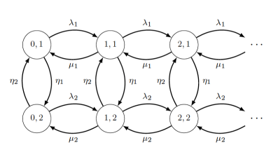
Figure 1: The state diagram of the Markov chain ${\bf N}(t)$.

For a fixed $j\in\mathbb{N}_{0}$, we assume that the system is subject to random initial conditions given by a Bernoulli trial on the states $(j,1)$ and $(j,2)$. Indeed, for a given $p\in[0,1]$, recalling (2), we have

$$p_{n,1}(0)=p\,\delta_{n,j},\qquad p_{n,2}(0)=(1-p)\,\delta_{n,j},$$ (3)

where $\delta_{n,j}$ is the Kronecker’s delta.

From the specified assumptions we have the following forward Kolmogorov equations for the first operational regime:

$${dp_{0,1}(t)\over dt}=-(\lambda_{1}+\eta_{1})\,p_{0,1}(t)+\eta_{2}\,p_{0,2}(t)+\mu_{1}\,p_{1,1}(t),$$

$${dp_{n,1}(t)\over dt}=-(\lambda_{1}+\mu_{1}+\eta_{1})\,p_{n,1}(t)+\eta_{2}\,p_{n,2}(t)+\mu_{1}\,p_{n+1,1}(t)+\lambda_{1}\,p_{n-1,1}(t),$$

$$\hskip 256.0748ptn\in\mathbb{N},$$ (4)

and for the second operational regime:

$${dp_{0,2}(t)\over dt}=-(\lambda_{2}+\eta_{2})\,p_{0,2}(t)+\eta_{1}\,p_{0,1}(t)+\mu_{2}\,p_{1,2}(t)$$

$${dp_{n,2}(t)\over dt}=-(\lambda_{2}+\mu_{2}+\eta_{2})\,p_{n,2}(t)+\eta_{1}\,p_{n,1}(t)+\mu_{2}\,p_{n+1,2}(t)+\lambda_{2}\,p_{n-1,2}(t),$$

$$\hskip 256.0748ptn\in\mathbb{N}.$$ (5)

Clearly, for all $t\geq 0$ one has:

$$\sum_{n=0}^{+\infty}\bigl{[}p_{n,1}(t)+p_{n,2}(t)\bigr{]}=1.$$ (6)

2.1 Steady-state distribution

Let us now investigate the steady-state distribution of the two-environment $M/M/1$ queue. We will show that it can be expressed as a generalized mixture of two geometric distributions. Our approach is different from the analysis performed in [39], where the steady-state distribution is achieved through recursive formulas.

Let ${\bf N}=(N,\mathscr{E})$ be the two-dimensional random variable describing the number of customers and the environment of the system in the steady-state regime. We aim to determine the steady-state probabilities for the $M/M/1$ queue under the two environments, defined as

$$q_{n,i}=\mathbb{P}(N=n,\mathscr{E}=i)=\lim_{t\to+\infty}p_{n,i}(t),\qquad n\in\mathbb{N}_{0},\quad i=1,2.$$ (7)

From (4) and (5) one has the following difference equations:

$$-(\lambda_{1}+\eta_{1})\,q_{0,1}+\eta_{2}\,q_{0,2}+\mu_{1}\,q_{1,1}=0,$$

$$-(\lambda_{1}+\mu_{1}+\eta_{1})\,q_{n,1}+\eta_{2}\,q_{n,2}+\mu_{1}\,q_{n+1,1}+\lambda_{1}\,q_{n-1,1}=0,\qquad n\in\mathbb{N},$$

$$-(\lambda_{2}+\eta_{2})\,q_{0,2}+\eta_{1}\,q_{0,1}+\mu_{2}\,q_{1,2}=0,$$

$$-(\lambda_{2}+\mu_{2}+\eta_{2})\,q_{n,2}+\eta_{1}\,q_{n,1}+\mu_{2}\,q_{n+1,2}+\lambda_{2}\,q_{n-1,2}=0,\qquad n\in\mathbb{N}.$$

Hence, denoting by

$$G_{i}(z)=\mathbb{E}[z^{N}\mathbbm{1}_{\mathscr{E}=i}]=\sum_{n=0}^{+\infty}z^{n}q_{n,i},\qquad 0<z<1,\qquad i=1,2$$

the probability generating functions for the two environments in steady-state regime, one has:

$$G_{1}(z)={\eta_{2}\,\mu_{2}\,z\,q_{0,2}-\mu_{1}\,q_{0,1}\big{[}\lambda_{2}\,z^{2}-(\lambda_{2}+\mu_{2}+\eta_{2})\,z+\mu_{2}\big{]}\over P(z)},$$

(8)

$$G_{2}(z)={\eta_{1}\,\mu_{1}\,z\,q_{0,1}-\mu_{2}\,q_{0,2}\big{[}\lambda_{1}\,z^{2}-(\lambda_{1}+\mu_{1}+\eta_{1})\,z+\mu_{1}\big{]}\over P(z)},$$

where $P(z)$ is the following third-degree polynomial in $z$ (see Eq. (22) of [39]):

$$P(z)=\lambda_{1}\lambda_{2}z^{3}-\big{[}\lambda_{1}\lambda_{2}+\lambda_{1}\mu_{2}+\lambda_{1}\eta_{2}+\mu_{1}\lambda_{2}+\eta_{1}\lambda_{2}\big{]}z^{2}$$

$$\hskip 2.84544pt+\big{[}\lambda_{1}\mu_{2}+\mu_{1}\lambda_{2}+\mu_{1}\mu_{2}+\mu_{1}\eta_{2}+\eta_{1}\mu_{2}\big{]}z-\mu_{1}\mu_{2},\qquad 0<z<1.$$ (9)

By taking into account the normalization condition $G_{1}(1)+G_{2}(1)=1$, from (8) we get:

$$\mu_{1}\,q_{0,1}+\mu_{2}\,q_{0,2}={\eta_{1}(\mu_{2}-\lambda_{2})+\eta_{2}(\mu_{1}-\lambda_{1})\over\eta_{1}+\eta_{2}}\cdot$$ (10)

It is worth noting that Eq. (10) is a suitable extension of the classical condition for the $M/M/1$ queue in the steady-state, i.e.  $\mu\,q_{0}=\mu-\lambda$. Moreover, recalling that $\eta_{1}+\eta_{2}>0$, Eq. (10) shows that the existence of the equilibrium distribution is guaranteed if and only if one of the following cases holds:

(i) $\eta_{2}=0$ and $\lambda_{2}/\mu_{2}<1$,

(ii) $\eta_{1}=0$ and $\lambda_{1}/\mu_{1}<1$,

(iii) $\eta_{1}>0$, $\eta_{2}>0$ and $\eta_{1}(\mu_{2}-\lambda_{2})+\eta_{2}(\mu_{1}-\lambda_{1})>0$.

Hereafter, we consider separately the three cases.

$\bullet$ Case (i)

If $\eta_{2}=0$ and $\lambda_{2}/\mu_{2}<1$ one can easily prove that

$$q_{n,1}=0,\qquad q_{n,2}=\Bigl{(}1-{\lambda_{2}\over\mu_{2}}\Bigr{)}\,\Bigl{(}{\lambda_{2}\over\mu_{2}}\Bigr{)}^{n},\qquad n\in\mathbb{N}_{0}.$$ (11)

Therefore, a steady-state regime does not hold for the $M/M/1$ queue under the environment $\mathscr{E}=1$, whereas a geometric-distributed steady-state regime exists for $\mathscr{E}=2$. In conclusion, if $\eta_{2}=0$ and $\lambda_{2}/\mu_{2}<1$ then $N$ admits of a geometric steady-state distribution $q_{n}=q_{n,1}+q_{n,2}$ with parameter $\lambda_{2}/\mu_{2}$.

$\bullet$ Case (ii)

If $\eta_{1}=0$ and $\lambda_{1}/\mu_{1}<1$, similarly to case (i), one has

$$q_{n,1}=\Bigl{(}1-{\lambda_{1}\over\mu_{1}}\Bigr{)}\,\Bigl{(}{\lambda_{1}\over\mu_{1}}\Bigr{)}^{n},\qquad q_{n,2}=0,\qquad n\in\mathbb{N}_{0}.$$

Hence, in this case $N$ has a geometric steady-state distribution $q_{n}=q_{n,1}+q_{n,2}$ with parameter $\lambda_{1}/\mu_{1}$.

$\bullet$ Case (iii)

Let $\eta_{1}>0$, $\eta_{2}>0$ and $\eta_{1}(\mu_{2}-\lambda_{2})+\eta_{2}(\mu_{1}-\lambda_{1})>0$. These assumptions are in agreement with the conditions given in [39]. Denoting by $\xi_{1}$, $\xi_{2}$, $\xi_{3}$ the roots of $P(z)$, given in (9), one has

$$\xi_{1}+\xi_{2}+\xi_{3}={\lambda_{1}\lambda_{2}+\lambda_{1}\mu_{2}+\lambda_{1}\eta_{2}+\lambda_{2}\mu_{1}+\lambda_{2}\eta_{1}\over\lambda_{1}\lambda_{2}},$$

$$\xi_{1}\xi_{2}+\xi_{1}\xi_{3}+\xi_{2}\xi_{3}={\lambda_{1}\mu_{2}+\lambda_{2}\mu_{1}+\mu_{1}\mu_{2}+\mu_{1}\eta_{2}+\mu_{2}\eta_{1}\over\lambda_{1}\lambda_{2}},$$ (12)

$$\xi_{1}\xi_{2}\xi_{3}={\mu_{1}\mu_{2}\over\lambda_{1}\lambda_{2}},$$

so that $\xi_{1}+\xi_{2}+\xi_{3}>0$, $\xi_{1}\xi_{2}+\xi_{1}\xi_{3}+\xi_{2}\xi_{3}>0$ and $\xi_{1}\xi_{2}\xi_{3}>0$. Moreover, we note that

$$(\xi_{1}-1)(\xi_{2}-1)(1-\xi_{3})={\eta_{1}(\mu_{2}-\lambda_{2})+\eta_{2}(\mu_{1}-\lambda_{1})\over\lambda_{1}\lambda_{2}}>0,$$ (13)

and that, due to (9),

$$P(0)=-\mu_{1}\mu_{2}<0,\qquad P(1)=\eta_{1}(\mu_{2}-\lambda_{2})+\eta_{2}(\mu_{1}-\lambda_{1})>0,$$

(14)

$$P\Big{(}\frac{\mu_{1}}{\lambda_{1}}\Big{)}=\frac{\eta_{1}\mu_{1}\lambda_{2}}{\lambda_{1}}\Big{(}\frac{\mu_{2}}{\lambda_{2}}-\frac{\mu_{1}}{\lambda_{1}}\Big{)},\qquad P\Big{(}\frac{\mu_{2}}{\lambda_{2}}\Big{)}=\frac{\eta_{2}\mu_{2}\lambda_{1}}{\lambda_{2}}\Big{(}\frac{\mu_{1}}{\lambda_{1}}-\frac{\mu_{2}}{\lambda_{2}}\Big{)}.$$

Hence, $P(z)$ has three positive roots, two of them greater than 1 and one less than 1. Hereafter we show that the present method allows us to express the distribution of interest in closed form, as a generalized mixture of geometric distributions. Hence, we assume that $\xi_{1}>1$, $\xi_{2}>1$ and $0<\xi_{3}<1$, and thus $P(z)=\lambda_{1}\lambda_{2}(z-\xi_{1})(z-\xi_{2})(z-\xi_{3})$.

Proposition 1

If $\eta_{1}>0$, $\eta_{2}>0$ and $\eta_{1}(\mu_{2}-\lambda_{2})+\eta_{2}(\mu_{1}-\lambda_{1})>0$, then the joint steady-state probabilities of ${\bf N}=(N,\mathscr{E})$ can be expressed in terms of the roots $\xi_{1}>1$, $\xi_{2}>1$ and $0<\xi_{3}<1$ of the polynomial (9) as follows:

$$q_{n,i}={\eta_{3-i}\over\eta_{1}+\eta_{2}}\Bigl{[}A_{i}\,\mathbb{P}(V_{1}=n)+(1-A_{i})\,\mathbb{P}(V_{2}=n)\Bigr{]},\qquad n\in\mathbb{N}_{0},i=1,2,$$ (15)

where $P(V_{i}=n)=(1-1/\xi_{i})(1/\xi_{i})^{n}$ $\;(n\in\mathbb{N}_{0},\;i=1,2)$ and

$$A_{i}={\xi_{1}\xi_{3}\bigl{[}\eta_{1}(\mu_{2}-\lambda_{2})+\eta_{2}(\mu_{1}-\lambda_{1})\bigr{]}\over\lambda_{i}\mu_{i}(1-\xi_{3})(\xi_{1}-1)(\xi_{1}-\xi_{2})}\,{\mu_{i}-\lambda_{i}\xi_{2}\over\mu_{3-i}-\lambda_{3-i}\xi_{3}},\quad i=1,2.$$ (16)

• Since $P(\xi_{3})=0$, to ensure the convergence of the probability generating functions (8), we impose that their numerators tend to zero as $z\to\xi_{3}$. Hence, by virtue of (10), one has (see also Eqs. (26) and (27) of [39]):

  $$q_{0,1}={\eta_{2}\xi_{3}\over\mu_{1}(1-\xi_{3})(\mu_{2}-\lambda_{2}\xi_{3})}\;{\eta_{1}(\mu_{2}-\lambda_{2})+\eta_{2}(\mu_{1}-\lambda_{1})\over\eta_{1}+\eta_{2}},$$

  (17)

  $$q_{0,2}={\eta_{1}\xi_{3}\over\mu_{2}(1-\xi_{3})(\mu_{1}-\lambda_{1}\xi_{3})}\;{\eta_{1}(\mu_{2}-\lambda_{2})+\eta_{2}(\mu_{1}-\lambda_{1})\over\eta_{1}+\eta_{2}}\cdot$$

  Note that, due to (12), (13) and (14), one has $\xi_{3}\neq\mu_{1}/\lambda_{1}$ and $\xi_{3}\neq\mu_{2}/\lambda_{2}$. Making use of (17), from (8) one finally obtains:

  $$G_{1}(z)={\eta_{2}\bigl{[}\eta_{1}(\mu_{2}-\lambda_{2})+\eta_{2}(\mu_{1}-\lambda_{1})\bigr{]}\over(1-\xi_{3})(\mu_{2}-\lambda_{2}\xi_{3})(\eta_{1}+\eta_{2})}\;{\mu_{2}-\lambda_{2}\xi_{3}\,z\over\lambda_{1}\lambda_{2}(z-\xi_{1})(z-\xi_{2})},$$

  (18)

  $$G_{2}(z)={\eta_{1}\bigl{[}\eta_{1}(\mu_{2}-\lambda_{2})+\eta_{2}(\mu_{1}-\lambda_{1})\bigr{]}\over(1-\xi_{3})(\mu_{1}-\lambda_{1}\xi_{3})(\eta_{1}+\eta_{2})}\;{\mu_{1}-\lambda_{1}\xi_{3}\,z\over\lambda_{1}\lambda_{2}(z-\xi_{1})(z-\xi_{2})}.$$

  Expanding $G_{1}(z)$ and $G_{2}(z)$, given in (18), in power series of $z$, one finally is led to

  $$q_{n,1}={\eta_{2}\xi_{3}\over\mu_{1}(1-\xi_{3})(\mu_{2}-\lambda_{2}\xi_{3})}\;{\eta_{1}(\mu_{2}-\lambda_{2})+\eta_{2}(\mu_{1}-\lambda_{1})\over\eta_{1}+\eta_{2}}$$

  $$\hskip 14.22636pt\times{1\over(\xi_{1}\xi_{2})^{n}}\Bigl{\{}{\xi_{1}^{n+1}-\xi_{2}^{n+1}\over\xi_{1}-\xi_{2}}-{\mu_{1}\over\lambda_{1}}\;{\xi_{1}^{n}-\xi_{2}^{n}\over\xi_{1}-\xi_{2}}\Bigr{\}},\qquad n\in\mathbb{N}_{0},$$

  (19)

  $$q_{n,2}={\eta_{1}\xi_{3}\over\mu_{2}(1-\xi_{3})(\mu_{1}-\lambda_{1}\xi_{3})}\;{\eta_{1}(\mu_{2}-\lambda_{2})+\eta_{2}(\mu_{1}-\lambda_{1})\over\eta_{1}+\eta_{2}}$$

  $$\hskip 14.22636pt\times{1\over(\xi_{1}\xi_{2})^{n}}\Bigl{\{}{\xi_{1}^{n+1}-\xi_{2}^{n+1}\over\xi_{1}-\xi_{2}}-{\mu_{2}\over\lambda_{2}}\;{\xi_{1}^{n}-\xi_{2}^{n}\over\xi_{1}-\xi_{2}}\Bigr{\}},\qquad n\in\mathbb{N}_{0}.$$

  From (19) one obtains immediately (15). $\Box$

We note that if $\eta_{1}(\mu_{2}-\lambda_{2})+\eta_{2}(\mu_{1}-\lambda_{1})>0$, the steady-state probabilities do not depend on the initial conditions (3), i.e. on the probability $p$.

By virtue of (13), from (18) one obtains (cf. also Eqs. (17) of [39]):

$$\mathbb{P}(\mathscr{E}=i)\equiv G_{i}(1)=\sum_{n=0}^{+\infty}q_{n,i}={\eta_{3-i}\over\eta_{1}+\eta_{2}},\qquad i=1,2.$$ (20)

From Proposition 1, we have that $\mathbb{P}(N=n|\mathscr{E}=1)$ and $\mathbb{P}(N=n|\mathscr{E}=2)$ $(n\in\mathbb{N}_{0})$ are both generalized mixtures of two geometric probability distributions of parameters $1/\xi_{1}$ and $1/\xi_{2}$, respectively (see Navarro [34] for details on generalized mixtures).

Making use of Proposition 1 and of (20), we determine the conditional means in a straightforward manner:

$$\mathbb{E}[N|\mathscr{E}=i]=\sum_{n=1}^{+\infty}n{q_{n,i}\over\mathbb{P}(\mathscr{E}=i)}={A_{i}\over\xi_{1}-1}+{1-A_{i}\over\xi_{2}-1},\qquad i=1,2.$$ (21)

Corollary 1

Under the assumptions of Proposition 1, for $n\in\mathbb{N}_{0}$ one obtains the steady-state probabilities of $N$:

$$q_{n}=q_{n,1}+q_{n,2}={\eta_{2}A_{1}+\eta_{1}A_{2}\over\eta_{1}+\eta_{2}}\mathbb{P}(V_{1}=n)+\Bigl{[}1-{\eta_{2}A_{1}+\eta_{1}A_{2}\over\eta_{1}+\eta_{2}}\Bigr{]}\mathbb{P}(V_{2}=n),$$ (22)

where $A_{1}$ and $A_{2}$ are provided in (16).

Eq. (22) shows that also $q_{n}$ is a generalized mixture of two geometric probability distributions of parameters $1/\xi_{1}$ and $1/\xi_{2}$, respectively, so that

$$\mathbb{E}(N)={\eta_{2}A_{1}+\eta_{1}A_{2}\over\eta_{1}+\eta_{2}}{1\over\xi_{1}-1}+\Bigl{[}1-{\eta_{2}A_{1}+\eta_{1}A_{2}\over\eta_{1}+\eta_{2}}\Bigr{]}{1\over\xi_{2}-1}\cdot$$ (23)

This result is in agreement with Eq. (33) of [39].

Figure 2 shows the steady-state probabilities $q_{n,1},q_{n,2}$ (on the left) and $q_{n}=q_{n,1}+q_{n,2}$ (on the right), obtained via Proposition 1 and Corollary 1, for $\lambda_{1}=1$, $\mu_{1}=0.5$, $\lambda_{2}=1$, $\mu_{2}=2$, $\eta_{1}=0.1$ and $\eta_{2}=0.08$. The roots of polynomial (9) can be evaluated by means of MATHEMATICA^®, so that $\xi_{1}=2.16716$, $\xi_{2}=1.08919$, $\xi_{3}=0.423647$.

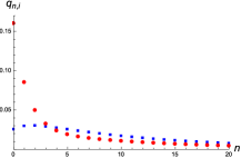
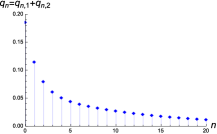
Figure 2: Plots of probabilities $q_{n,1}$ (square) and $q_{n,2}$ (circle), on the left, and $q_{n}=q_{n,1}+q_{n,2}$, on the right, for $\lambda_{1}=1$, $\mu_{1}=0.5$, $\lambda_{2}=1$, $\mu_{2}=2$, $\eta_{1}=0.1$ and $\eta_{2}=0.08$.

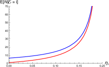
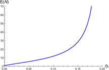
Figure 3: For $\lambda_{1}=1$, $\mu_{1}=0.5$, $\lambda_{2}=1$, $\mu_{2}=2$, $\eta_{1}=0.1$ and $0\leq\eta_{2}<0.2$ the conditional means $\mathbb{E}[N|\mathscr{E}=i]$, given in (21), are plotted on the left for $i=1$ (top) and $i=2$ (bottom), whereas the mean $\mathbb{E}(N)$ is plotted on the right.

Figure 3 gives, on the left, a plot of the conditional means, obtained in (21), for a suitable choice of the parameters, showing that $\mathbb{E}[N|\mathscr{E}=i]$ is increasing in $\eta_{2}$, for $i=1,2$. The mean $\mathbb{E}(N)$, obtained via (23), is plotted as function of $\eta_{2}$ on the right of Figure 3.

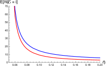
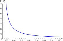
Figure 4: For $\lambda_{1}=1$, $\mu_{1}=0.5$, $\lambda_{2}=1$, $\mu_{2}=2$, $\eta_{2}=0.1$ and $\eta_{1}>0.05$ the conditional means $\mathbb{E}[N|\mathscr{E}=i]$, given in (21), are plotted on the left for $i=1$ (top) and $i=2$ (bottom), whereas the mean $\mathbb{E}(N)$ is plotted on the right.

Similarly, on the left of Figure 4 are plotted the conditional means for a suitable choice of the parameters, showing that $\mathbb{E}[N|\mathscr{E}=i]$ is decreasing in $\eta_{1}$, for $i=1,2$. The mean $\mathbb{E}(N)$ is plotted as function of $\eta_{1}$ on the right of Figure 4.

We remark that in the cases considered in Figures 3 and 4, the parameters satisfy the condition $\eta_{1}(\mu_{2}-\lambda_{2})+\eta_{2}(\mu_{1}-\lambda_{1})>0$, and thus the joint steady-state probabilities of ${\bf N}$ there exist due to Proposition 1. Moreover, in the cases considered in Figures 3 and 4, one has $\lambda_{1}>\mu_{1}$ and $\lambda_{2}<\mu_{2}$, so that in absence of switching the queue should not admit a steady-state regime in the first environment, whereas a steady-state regime should hold in the second environment. This example shows that the switching mechanism is useful to obtain stationarity, in the sense that the alternating $M/M/1$ queue may admit a steady-state regime even if one of the alternating environments does not.

Making use of Proposition 1 and Eq. (20) it is easy to determine the (Shannon) entropies

$$H[N|\mathscr{E}=i]=-\sum_{n=1}^{+\infty}\frac{q_{n,i}}{\mathbb{P}(\mathscr{E}=i)}\log\Big{[}\frac{q_{n,i}}{\mathbb{P}(\mathscr{E}=i)}\Big{]},\qquad i=1,2,$$ (24)

$$H(N)=-\sum_{n=1}^{+\infty}q_{n}\log q_{n},$$ (25)

where ‘$\log$’ means natural logarithm.

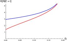
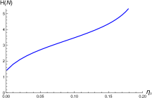
Figure 5: On the left, the conditional entropy $H[N|\mathscr{E}=i]$, given in (24), is plotted with $\lambda_{1}=1$, $\mu_{1}=0.5$, $\lambda_{2}=1$, $\mu_{2}=2$, $\eta_{1}=0.1$ and $0\leq\eta_{2}<0.2$, for $i=1$ (top) and $i=2$ (bottom). On the right, the entropy $H(N)$, given in (25), is plotted for the same choices of parameters.

The conditional entropy (24) is a measure of interest in queueing, since it gives the average amount of information that is gained when the steady-state number of customers $N$ in the queue is observed given that the system is in environment $\mathscr{E}=i$. In Figure 5 we plot the conditional entropy (24) (on the left) and the entropy (25) (on the right) for the same case of Figure 3, showing that $H[N|\mathscr{E}=i]$ $(i=1,2)$ and $H[N)$ are increasing in $\eta_{2}$. Furthermore, for the same choices of Figure 4, in Figure 6 the entropies $H[N|\mathscr{E}=i]$ $(i=1,2)$ and $H[N)$ are plotted, showing that are decreasing in $\eta_{1}$.

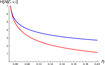
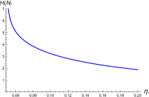
Figure 6: On the left, $H[N|\mathscr{E}=i]$ is plotted with $\lambda_{1}=1$, $\mu_{1}=0.5$, $\lambda_{2}=1$, $\mu_{2}=2$, $\eta_{2}=0.1$ and $\eta_{1}>0.05$, for $i=1$ (top) and $i=2$ (bottom). On the right, $H(N)$ is plotted for the same choices of parameters.

Moreover, recalling (15), (20) and (22) one can also define the following entropies

$$H[\mathscr{E}|N=n]=-\sum_{i=1}^{2}{q_{n,i}\over q_{n}}\log{q_{n,i}\over q_{n}},\qquad n\in\mathbb{N}_{0},$$ (26)

$$H(\mathscr{E})=-\sum_{i=1}^{2}{\eta_{3-i}\over\eta_{1}+\eta_{2}}\log{\eta_{3-i}\over\eta_{1}+\eta_{2}}$$ (27)

Note that $0\leq H[\mathscr{E}|N=n]\leq\log 2$ and $0\leq H(\mathscr{E})\leq\log 2$. The conditional entropy (26) gives the average amount of information on the environment when the number of customers $N=n$ in the queue is observed, whereas the entropy (27) gives the average amount of information on the environment. Note that, under the assumptions of Proposition 1, from (26) one has

$$H_{\infty}=\lim_{n\to+\infty}H[\mathscr{E}|N=n]$$

$$=-\sum_{i=1}^{2}{\eta_{3-i}\,(1-A_{i})\over\eta_{1}\,(1-A_{2})+\eta_{2}\,(1-A_{1})}\log{\eta_{3-i}\,(1-A_{i})\over\eta_{1}\,(1-A_{2})+\eta_{2}\,(1-A_{1})},$$ (28)

with $A_{i}$ defined in (16). Therefore, the conditional average amount of information on the environment tends to the value given in (28) when the number of customers increases.

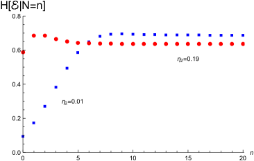
(a) $\eta_{1}=0.1$

(b) $\eta_{2}=0.1$

Figure 7: Plots of $H[\mathscr{E}|N=n]$ for $\lambda_{1}=1.0,\mu_{1}=0.5,\lambda_{2}=1,\mu_{2}=2.0$ and $n=1,2,\ldots,20$, with different choices of $\eta_{1},\eta_{2}$.

In Figure 7 the conditional entropies (26) are shown for some choices of parameters. In particular, in Figure 7(a) $H[\mathscr{E}|N=0]=0.0923799$, $H_{\infty}=0.686201$ and $H(\mathscr{E})=0.304636$ for $\eta_{2}=0.01$, whereas when $\eta_{2}=0.19$ one has $H[\mathscr{E}|N=0]=0.5898$, $H_{\infty}=0.639399$ and $H(\mathscr{E})=0.644186$. Furthermore, in Figure 7(b) one has $H[\mathscr{E}|N=0]=0.473177$, $H_{\infty}=0.643289$ and $H(\mathscr{E})=0.661563$ for $\eta_{1}=0.06$, whereas when $\eta_{1}=0.6$ it results $H[\mathscr{E}|N=0]=0.281199$, $H_{\infty}=0.613038$ and $H(\mathscr{E})=0.410116$. From Figure 7, we note that if $\eta_{1}>\eta_{2}$ then $H[\mathscr{E}|N=0]<H(\mathscr{E})<H_{\infty}$, whereas when $\eta_{1}<\eta_{2}$ it follows $H[\mathscr{E}|N=0]<H_{\infty}<H(\mathscr{E})$.

3 Analysis of case $\eta_{2}=0$

In the general case it is hard to determine the transient distribution of ${\bf N}(t)$. Hence, we limit ourselves to the analysis of the system with $\eta_{2}=0$ and with the initial state given in (2). Figure 8 shows the state diagram of ${\bf N}(t)$ in this special case, where only transitions from the first to the second environment are allowed.

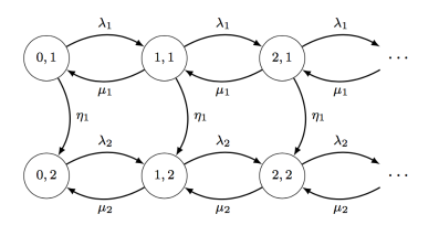
Figure 8: The state diagram of the Markov chain ${\bf N}(t)$ when $\eta_{2}=0$.

We remark that, the case $\eta_{1}=0$ can be studied similarly by symmetry.

3.1 Transient probabilities

Hereafter, we express the transient probabilities (1) in terms of the analogue probabilities $\widehat{p}_{j,n}^{(i)}(t)$ of two $M/M/1$ queueing systems $\widehat{N}^{(i)}(t)$, $t\geq 0$, $i=1,2$, characterized by arrival rate $\lambda_{i}$ and service rate $\mu_{i}$. Note that, for $j,n\in\mathbb{N}_{0}$, $t\geq 0$ and $i=1,2$, we have (see, e.g., Zhang and Coyle [40], or Eq. (32) of Giorno et al. [23])

$$\widehat{p}_{j,n}^{(i)}(t) = e^{-(\lambda_{i}+\mu_{i})t}\Big{\{}\Big{(}\frac{\lambda_{i}}{\mu_{i}}\Big{)}^{(n-j)/2}I_{n-j}(2t\sqrt{\lambda_{i}\mu_{i}})$$

$$+ \Big{(}\frac{\lambda_{i}}{\mu_{i}}\Big{)}^{(n-j-1)/2}I_{n+j+1}(2t\sqrt{\lambda_{i}\mu_{i}})$$

$$+ \Big{(}1-\frac{\lambda_{i}}{\mu_{i}}\Big{)}\Big{(}\frac{\lambda_{i}}{\mu_{i}}\Big{)}^{n}\sum_{k=n+j+2}^{\infty}\Big{(}\frac{\mu_{i}}{\lambda_{i}}\Big{)}^{k/2}I_{k}(2t\sqrt{\lambda_{i}\mu_{i}})\Big{\}},$$

where $I_{\nu}(z)$ denotes the modified Bessel function of the first kind. Moreover, making use of Eq. (49), pag. 237, of Erdélyi et al. [20], for $n\in\mathbb{N}_{0}$, $t\geq 0$ and $i=1,2$, we have

$$\widehat{p}_{0,n}^{(i)}(t)=\frac{1}{\mu_{i}}\Big{(}\frac{\lambda_{i}}{\mu_{i}}\Big{)}^{n}\frac{1}{t}e^{-(\lambda_{i}+\mu_{i})t}\sum_{k=n+1}^{\infty}k\Big{(}\frac{\lambda_{i}}{\mu_{i}}\Big{)}^{k/2}I_{k}(2t\sqrt{\lambda_{i}\mu_{i}}).$$ (30)

Proposition 2

Let $\eta_{2}=0$. For all $t\geq 0$ and $j,n\in\mathbb{N}_{0}$, the transition probabilities of ${\bf N}(t)$ can be expressed as:

$$p_{n,1}(t)=p\,e^{-\eta_{1}t}\widehat{p}_{j,n}^{(1)}(t),$$ (31)

$$p_{n,2}(t)=(1-p)\,\widehat{p}_{j,n}^{(2)}(t)+p\,\eta_{1}\sum_{k=0}^{+\infty}\int_{0}^{t}e^{-\eta_{1}\,\tau}\,\widehat{p}_{j,k}^{(1)}(\tau)\,\widehat{p}_{k,n}^{(2)}(t-\tau)\;d\tau,$$ (32)

where $\widehat{p}_{j,n}^{(i)}(t)$ are provided in (3.1) and (30).

• It follows from (4) and (5), recalling the initial conditions (3). $\Box$

In the case $\eta_{2}=0$, at most one switch can occur (from environment 1 to environment 2). Hence, Eq. (31) is also obtainable by noting that $p_{n,1}(t)$ can be viewed as the probability that process ${\bf N}(t)$ is located at $(n,1)$ at time $t$, starting from $(j,1)$ at time $0$, with probability $p$, and that no ‘switches’ occurred up to time $t$. Similarly, resorting to the total probability law, Eq. (32) is recovered by taking into account that process ${\bf N}(t)$ is located at $(n,2)$ at time $t$ in two cases:

- when starting from $(j,2)$ at time $0$, with probability $1-p$, and performing a transition from $(j,2)$ to $(n,2)$ at time $t$,

- when starting from $(j,1)$ at time $0$, with probability $p$, then performing a transition from $(j,1)$ to $(k,1)$ at time $\tau$ (with $k\in\mathbb{N}_{0}$ and $0<\tau<t$), then switching from environment 1 to environment 2 at time $\tau$, and finally performing a transition from state $(k,2)$ to $(n,2)$ in the time interval $(\tau,t)$.

3.2 First-passage time problems

We now analyze the first-passage time through zero state of the system when $\eta_{2}=0$. To this aim, first we define a new two-dimensional stochastic process $\{\widetilde{\bf N}(t)=[\widetilde{N}(t),{\mathscr{E}}(t)],t\geq 0\}$ whose state diagram is given in Figure 9. This process is obtained from ${\bf N}(t)$ by removing all the transitions from $(0,i)$, $i=1,2$. In this case only transitions from the first to the second environment are allowed. Moreover, $(0,1)$ and $(0,2)$ are absorbing states for the process $\widetilde{\bf N}(t)$.

Figure 9: The state diagram of the birth-death process for the busy period.

We denote by

$$\gamma_{n,i}(t)=\mathbb{P}[\widetilde{\bf N}(t)=(n,i)],\qquad n\in\mathbb{N}_{0},\quad i=1,2,\quad t\geq 0$$ (33)

the state probabilities of the new process, where

$$\widetilde{\bf N}(0)=\left\{\begin{array}[]{ll}(j,1),&\;{\rm with\;probability}\;p,\\ (j,2),&\;{\rm with\;probability}\;1-p.\end{array}\right.$$ (34)

Since $\eta_{2}=0$ the following equations hold:

$${d\gamma_{0,1}(t)\over dt}=\mu_{1}\,\gamma_{1,1}(t),$$

$${d\gamma_{1,1}(t)\over dt}=-(\lambda_{1}+\mu_{1}+\eta_{1})\,\gamma_{1,1}(t)+\mu_{1}\,\gamma_{2,1}(t),$$ (35)

$${d\gamma_{n,1}(t)\over dt}=-(\lambda_{1}+\mu_{1}+\eta_{1})\,\gamma_{n,1}(t)+\mu_{1}\,\gamma_{n+1,1}(t)+\lambda_{1}\,\gamma_{n-1,1}(t),$$

$$\hskip 227.62204ptn=2,3,\ldots$$

and

$${d\gamma_{0,2}(t)\over dt}=\mu_{2}\,\gamma_{1,2}(t),$$

$${d\gamma_{1,2}(t)\over dt}=-(\lambda_{2}+\mu_{2})\,\gamma_{1,2}(t)+\eta_{1}\,\gamma_{1,1}(t)+\mu_{2}\,\gamma_{2,2}(t),$$ (36)

$${d\gamma_{n,2}(t)\over dt}=-(\lambda_{2}+\mu_{2})\,\gamma_{n,2}(t)+\eta_{1}\,\gamma_{n,1}(t)+\mu_{2}\,\gamma_{n+1,2}(t)+\lambda_{2}\,\gamma_{n-1,2}(t),$$

$$\hskip 227.62204ptn=2,3,\ldots,$$

with initial conditions

$$\gamma_{n,1}(0)=p\,\delta_{n,j},\qquad\gamma_{n,2}(0)=(1-p)\,\delta_{n,j}\qquad(0\leq p\leq 1).$$ (37)

In order to obtain suitable relations for the state probabilities (33), we recall that the transition probabilities avoiding state 0 for the $M/M/1$ queue with arrival rate $\lambda_{i}$ and service rate $\mu_{i}$, for $j,n\in\mathbb{N}$ and $t>0$ is (cf. Abate et al. [1])

$$\widehat{\alpha}_{j,n}^{(i)}(t)=e^{-(\lambda_{i}+\mu_{i})t}\Big{(}\frac{\lambda_{i}}{\mu_{i}}\Big{)}^{(n-j)/2}\,\left[I_{n-j}(2t\sqrt{\lambda_{i}\mu_{i}})-I_{n+j}(2t\sqrt{\lambda_{i}\mu_{i}})\right]$$ (38)

and, due to relation $I_{j-1}(z)-I_{j+1}(z)=2j\,I_{j}(z)/z$ (cf. Eq. 8.486.1, p. 928 of [24]),

$$\widehat{\alpha}_{j,1}^{(i)}(t)={j\over\mu_{i}\,t}\,e^{-(\lambda_{i}+\mu_{i})t}\Big{(}{\mu_{i}\over\lambda_{i}}\Big{)}^{j/2}I_{j}(2t\sqrt{\lambda_{i}\mu_{i}}).$$ (39)

Proposition 3

If $\eta_{2}=0$, for $j\in\mathbb{N}$, $n\in\mathbb{N}_{0}$ and $t>0$, for the state probabilities (33) one has:

$$\gamma_{n,1}(t)=p\,e^{-\eta_{1}t}\,\widehat{\alpha}_{j,n}^{(1)}(t),$$ (40)

$$\gamma_{n,2}(t)=(1-p)\,\widehat{\alpha}_{j,n}^{(2)}(t)+\eta_{1}p\sum_{k=1}^{\infty}\int_{0}^{t}e^{-\eta_{1}\tau}\,\widehat{\alpha}_{j,k}^{(1)}(\tau)\,\widehat{\alpha}_{k,n}^{(2)}(t-\tau)\;d\tau,$$ (41)

where $\widehat{\alpha}_{j,k}^{(i)}(t)$ are given in (38) and (39).

• It follows from (35) and (36), recalling the initial conditions (37).

  $\Box$

The term in the right-hand-side of (40) can be interpreted as follows: starting from $(j,1)$ at time 0, with probability $p$, the process reaches $(n,1)$, with $n\in\mathbb{N}$, at time $t$ without crossing $(0,1)$ in the interval $(0,\tau)$, and no switches occurred up to time $t$. Instead, the 2 terms in the right-hand-side of (41) have the following meaning:

- starting from $(j,2)$ at time 0, with probability $1-p$, the process reaches $(n,2)$ at time $t$, with $n\in\mathbb{N}$, at time $t$ without crossing $(0,2)$ in the interval $(0,\tau)$;

- starting from $(j,1)$ at time 0, with probability $p$, the process reaches $(k,1)$, with $k\in\mathbb{N}$, at time $\tau\in(0,t)$ without crossing $(0,1)$ in the interval $(0,\tau)$, then a switch occurs at time $t$, and starting from $(k,2)$ the process reaches $(n,2)$ at time $t$ without crossing $(0,2)$ in the interval $(\tau,t)$.

For $j\in\mathbb{N}$, we consider the random variable

$$T_{j}=\inf\{t>0:{\bf N}(t)=(0,1)\;{\rm or}\;{\bf N}(t)=(0,2)\},$$

where ${\bf N}(0)$ is given in (2), with $j\in\mathbb{N}$. Note that $T_{j}$ denotes the first-passage time (FPT) of the process ${\bf N}(t)$ through zero starting from $(j,1)$ with probability $p$ and from $(j,2)$ with probability $1-p$, with $j\in\mathbb{N}$. Hence, $T_{j}$ is the first emptying time of the queue, with the initial state specified in (2). For $\eta_{2}=0$, the FPT of ${\bf N}(t)$ through $(0,1)$ or $(0,2)$ is identically distributed as the FPT of $\widetilde{\bf N}(t)$ through the same states. Therefore, the first passage through $(0,1)$ or $(0,2)$ for ${\bf N}(t)$ can be studied via the probabilities obtained in Proposition 3. Specifically, recalling (33), for $j\in\mathbb{N}$ we have:

$$\mathbb{P}(T_{j}<t)+\sum_{n=1}^{+\infty}\bigl{[}\gamma_{n,1}(t)+\gamma_{n,2}(t)\bigr{]}=1.$$ (42)

We focus our attention on the FPT probability density

$$b_{j}(t)={d\over dt}\,\mathbb{P}(T_{j}<t),\qquad t>0,\;j\in\mathbb{N}.$$ (43)

Hereafter we show that such density can be expressed in terms of the first-passage-time density from state $j\in\mathbb{N}$ to state 0 of the $M/M/1$ queues with rates $\lambda_{i}$ and $\mu_{i}$, $i=1,2$, given by (see, for instance, [1]):

$$\widehat{g}_{j,0}^{(i)}(t)=\frac{j}{t}\,e^{-(\lambda_{i}+\mu_{i})t}\Big{(}\frac{\mu_{i}}{\lambda_{i}}\Big{)}^{j/2}\,I_{j}(2t\sqrt{\lambda_{i}\mu_{i}}),\qquad t>0.$$ (44)

Proposition 4

If $\eta_{2}=0$, for $t>0$ FPT probability density (43) is expressed as:

$$b_{j}(t)=p\,e^{-\eta_{1}t}\,\widehat{g}_{j,0}^{(1)}(t)+(1-p)\,\widehat{g}_{j,0}^{(2)}(t)$$

$$\hskip 28.45274pt+\eta_{1}p\sum_{k=1}^{\infty}\int_{0}^{t}e^{-\eta_{1}\tau}\,\widehat{\alpha}_{j,k}^{(1)}(\tau)\,\widehat{g}_{k,0}^{(2)}(t-\tau)\;d\tau,\qquad j\in\mathbb{N},$$ (45)

where $\widehat{g}_{k,0}^{(i)}(t)$ is the FPT density given in (44).

• Making use of (35) and (36) one has

  $${d\over dt}\sum_{n=1}^{+\infty}\gamma_{n,i}(t)=-\mu_{i}\gamma_{1,i}(t)+(-1)^{i}\eta_{1}\sum_{n=1}^{+\infty}\gamma_{n,1}(t),\qquad i=1,2,$$

  so that from (42) and (43) we obtain

  $$b_{j}(t)=\mu_{1}\,\gamma_{1,1}(t)+\mu_{2}\,\gamma_{1,2}(t),\qquad t>0,\;j\in\mathbb{N}.$$ (46)

  Due to Proposition 3, from (46) for $j\in\mathbb{N}$ it follows:

  $$b_{j}(t)=\mu_{1}\,p\,e^{-\eta_{1}t}\,\widehat{\alpha}_{j,1}^{(1)}(t)+\mu_{2}\,(1-p)\,\widehat{\alpha}_{j,1}^{(2)}(t)$$

  $$\hskip 34.14322pt+\mu_{2}\,\eta_{1}p\sum_{k=1}^{\infty}\int_{0}^{t}e^{-\eta_{1}\tau}\,\widehat{\alpha}_{j,k}^{(1)}(\tau)\,\widehat{\alpha}_{k,1}^{(2)}(t-\tau)\;d\tau,\qquad t>0.$$ (47)

  By virtue of (39) and (44) one has $\mu_{i}\,\widehat{\alpha}_{j,1}^{(i)}(t)=\widehat{g}_{j,0}^{(i)}(t)$ for $i=1,2$, so that (45) immediately follows from (47). $\Box$

For $j\in\mathbb{N}$, the 3 terms in the right-hand-side of the FPT density (45) can be interpreted as follows:

- starting from $(j,1)$ at time 0, with probability $p$, the process reaches $(0,1)$ for the first time at time $t$, and no switches occurred up to time $t$;

- starting from $(j,2)$ at time 0, with probability $1-p$, the process reaches $(0,2)$ for the first time at time $t$;

- starting from $(j,1)$ at time 0, with probability $p$, the process reaches $(k,1)$, with $k\in\mathbb{N}$, at time $\tau\in(0,t)$ without crossing $(0,1)$ in the interval $(0,\tau)$, then a switch occurs at time $t$, and starting from $(k,2)$ the process reaches $(0,2)$ for the first time at time $t$.

Let

$$B_{j}(s)={\cal L}[b_{j}(t)]=\int_{0}^{+\infty}e^{-s\,t}b_{j}(t)\;dt,\qquad s>0,j\in\mathbb{N}$$

be the Laplace transform of the FPT density $b_{j}(t)$.

Proposition 5

For $s>0$ and $j\in\mathbb{N}$, one has

$$B_{j}(s)={p\over[\varphi_{1}(s)]^{j}}+{1-p\over[\psi_{1}(s)]^{j}}+{\eta_{1}\,p\,\varphi_{2}(s)\over\lambda_{1}[\psi_{1}(s)-\varphi_{1}(s)]\,[\psi_{1}(s)-\varphi_{2}(s)]}$$

$$\hskip 14.22636pt\times{[\psi_{1}(s)]^{j}-[\varphi_{1}(s)]^{j}\over[\varphi_{1}(s)]^{j-1}[\psi_{1}(s)]^{j-1}},\qquad s>0,\;j\in\mathbb{N},$$ (48)

with

$$\varphi_{1}(s),\varphi_{2}(s)=\frac{s+\lambda_{1}+\mu_{1}+\eta_{1}\pm\sqrt{(s+\lambda_{1}+\mu_{1}+\eta_{1})^{2}-4\lambda_{1}\mu_{1}}}{2\mu_{1}},$$ (49)

for $0<\varphi_{2}(s)<1<\varphi_{1}(s)$, and

$$\psi_{1}(s),\psi_{2}(s)=\frac{s+\lambda_{2}+\mu_{2}\pm\sqrt{(s+\lambda_{2}+\mu_{2})^{2}-4\lambda_{2}\mu_{2}}}{2\mu_{2}},$$ (50)

for $0<\psi_{2}(s)<1<\psi_{1}(s)$.

The Laplace transform (48) is useful to calculate the probability that the process ${\bf N}(t)$ eventually reach the states $(0,1)$ or $(0,2)$ and the FPT moments.

Let us now determine the probability of the eventual first queue emptying. Since $\eta_{2}=0$, if $\lambda_{2}\leq\mu_{2}$ then $\psi_{1}(0)=1$, so that ${\mathbb{P}}(T_{j}<\infty)=1$, whereas if $\lambda_{2}>\mu_{2}$, then we have $\psi_{1}(0)=\lambda_{2}/\mu_{2}$, so that for $j\in\mathbb{N}$ it results:

$$\mathbb{P}(T_{j}<+\infty)=\int_{0}^{+\infty}b_{j}(t)\;dt=B_{j}(0)={p\over[\varphi_{1}(0)]^{j}}+(1-p)\Bigl{(}{\mu_{2}\over\lambda_{2}}\Bigr{)}^{j}$$

$$+{\eta_{1}\,p\,\varphi_{2}(0)\over\lambda_{1}[\varphi_{1}(0)-\lambda_{2}/\mu_{2}][\varphi_{2}(0)-\lambda_{2}/\mu_{2}]}\Bigl{(}{\mu_{2}\over\lambda_{2}}\Bigr{)}^{j-1}{(\lambda_{2}/\mu_{2})^{j}-[\varphi_{1}(0)]^{j}\over[\varphi_{1}(0)]^{j-1}}\cdot$$ (51)

Note that if $j=1$, $b_{1}(t)$ represents the busy period density of the considered queueing model; hence, if $\lambda_{2}\leq\mu_{2}$ the busy period termination is certain. On the contrary, if $\lambda_{2}>\mu_{2}$, (51) takes the simplest form:

$${\mathbb{P}}(T_{1}<+\infty)=\int_{0}^{+\infty}b_{1}(t)\;dt={p\over\varphi_{1}(0)}+{1-p\over\psi_{1}(0)}+{p\,\eta_{1}\varphi_{2}(0)\over\lambda_{1}[\psi_{1}(0)-\varphi_{2}(0)]}.$$

For $\lambda_{2}>\mu_{2}$, in Figure 10 we plot $\mathbb{P}(T_{j}<+\infty)$, given in (51), as function of $\eta_{2}$ for $j=1,3,5,10$. The case $j=1$ corresponds to the probability that the busy period ends.

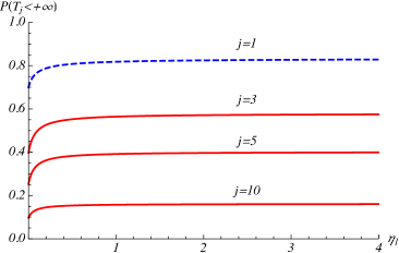
(a) $\lambda_{1}=1.0,\mu_{1}=0.5$

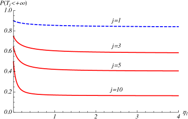
(b) $\lambda_{1}=0.5,\mu_{1}=1.0$

Figure 10: Plots of FPT probabilities $\mathbb{P}(T_{j}<+\infty)$ as function of $\eta_{1}$ for $\eta_{2}=0$, $\lambda_{2}=1.2$, $\mu_{2}=1.0$ and $p=0.4$.

When $\lambda_{2}<\mu_{2}$, $\eta_{1}>0$ and $j\in\mathbb{N}$, from (48) we obtain the FPT mean

$$\mathbb{E}(T_{j})={j\over\mu_{2}-\lambda_{2}}+p\,\biggl{[}1-{1\over[\varphi_{1}(0)]^{j}}\biggr{]}\,\biggl{[}{1\over(\lambda_{1}-\mu_{1}+\eta_{1})\varphi_{1}(0)-(\lambda_{1}-\mu_{1}-\eta_{1})}$$

$$\hskip 22.76228pt+{1\over(\lambda_{1}-\mu_{1}+\eta_{1})\varphi_{2}(0)-(\lambda_{1}-\mu_{1}-\eta_{1})}-{1\over\eta_{1}}\,{\mu_{1}-\lambda_{1}\over\mu_{2}-\lambda_{2}}\biggr{]}\cdot$$ (52)

Clearly, for $p=0$, the right-hand side of (52) corresponds to the FPT mean of the $M/M/1$ queue in the second environment.

Finally, in Figure 11 we plot the mean (52) as function of $\eta_{1}$; since $\lambda_{2}<\mu_{2}$, the first passage through zero state is a certain event.

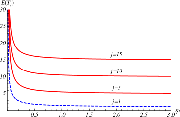
(a) $\lambda_{1}=1.0,\mu_{1}=0.5$

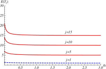
(b) $\lambda_{1}=0.5,\mu_{1}=1.0$

Figure 11: Plots of FPT mean $\mathbb{E}(T_{j})$ as function of $\eta_{1}$ for $\eta_{2}=0$, $\lambda_{2}=1.0$, $\mu_{2}=2.0$ and $p=0.4$.

4 Diffusion approximation

This section is devoted to the construction of a heavy-traffic diffusion approximation for the process ${\bf N}(t)$. As customary, we adopt a scaling procedure that is usual in queueing theory and in other contexts (c.f. Di Crescenzo et al. [15] or Dharmaraja et al. [11], for instance). As a first step, we perform a different parameterization of the arrival and service rates of the stochastic model introduced in Section 2. Specifically, we set

$$\lambda_{i}=\frac{\lambda_{i}^{*}}{\epsilon}+\frac{\omega_{i}^{2}}{2\epsilon^{2}},\qquad\mu_{i}=\frac{\mu_{i}^{*}}{\epsilon}+\frac{\omega_{i}^{2}}{2\epsilon^{2}}\qquad(i=1,2),$$ (53)

where $\lambda_{i}^{*}>0$, $\mu_{i}^{*}>0$, $\omega_{i}^{2}>0$, for $i=1,2$, and $\epsilon>0$. We remark that $\epsilon$ is a positive parameter that has a relevant role in the scaling procedure indicated below.

Let us now consider the position $N_{\epsilon}^{*}(t)=N(t)\epsilon$, for any $t>0$. Hence, the process $\{{\bf N}^{*}_{\epsilon}(t)=[N_{\epsilon}^{*}(t),\mathscr{E}(t)]=[N(t)\epsilon,\mathscr{E}(t)],t>0\}$ is a two-dimensional continuous-time Markov chain, having state-space $\mathbb{N}_{0,\epsilon}\times\{1,2\}$, where $\mathbb{N}_{0,\epsilon}=\{0,\epsilon,2\epsilon,\ldots\}$. We denote the transient probabilities of ${\bf N}^{*}_{\epsilon}(t)$, $t>0$, as

$$p_{\epsilon}(n,i;t)=\mathbb{P}[{\bf N}^{*}_{\epsilon}(t)=(n\epsilon,i)]=\mathbb{P}[n\epsilon\leq N_{\epsilon}^{*}(t)<(n+1)\epsilon,\mathscr{E}(t)=i)],$$ (54)

for $n\in\mathbb{N}_{0}$ and $i=1,2$. In the limit as $\epsilon\to 0^{+}$, it can be shown that the scaled process $N_{\epsilon}^{*}(t)$ converges weakly to a two-dimensional stochastic process, say $\{{\bf X}(t)=[X(t),\mathscr{E}(t)],t\geq 0\}$, having state-space $\mathbb{R}^{+}_{0}\times\{1,2\}$. Note that ${\bf X}(t)$ may be viewed as a restricted Wiener process alternating between two environments, with switching rates $\eta_{1}$ and $\eta_{2}$. For $x\in\mathbb{R}^{+}_{0}$, $t>0$ and $i=1,2$, let

$$f_{i}(x,t)=\frac{d}{dx}\,\mathbb{P}\{X(t)<x,\mathscr{E}(t)=i\}$$ (55)

denote the probability densities of the process ${\bf X}(t)$, where the initial state is

$${\bf X}(0)=\left\{\begin{array}[]{ll}(y,1),&\;{\rm with\;probability}\;p,\\ (y,2),&\;{\rm with\;probability}\;1-p,\end{array}\right.$$ (56)

with $y\in\mathbb{R}^{+}_{0}$. Starting from the forward equations for ${\bf N}(t)$, given in Eqs. (4) and (5), the scaling procedure mentioned above yields that the densities (55) satisfy the following partial differential equations of Kolmogorov type, for $i=1,2$, $x\in\mathbb{R}^{+}$ and $t>0$:

$$\frac{\partial f_{i}(x,t)}{\partial t}=-(\lambda_{i}^{*}-\mu_{i}^{*})\frac{\partial f_{i}(x,t)}{\partial x}+\frac{\omega_{i}^{2}}{2}\frac{\partial^{2}f_{i}(x,t)}{\partial x^{2}}+\eta_{3-i}f_{3-i}(x,t)-\eta_{i}f_{i}(x,t).$$ (57)

We note that the first 2 terms in the right-hand-side of (57) correspond to the classical diffusive operators of a Wiener process, whereas the last 2 terms express the joking between the two different environments, occurring with switching rates $\eta_{1}$ and $\eta_{2}$. The first and second infinitesimal moments of the Wiener process in the $i$-th environment are respectively $\lambda_{i}^{*}-\mu_{i}^{*}$ and $\omega_{i}^{2}$, $i=1,2$. It is worth pointing out that, due to the scaling procedure, the first equations of systems (4) and (5) lead to the following reflecting condition at 0:

$$\lim_{x\to 0^{+}}\left[(\lambda_{i}^{*}-\mu_{i}^{*})f_{i}(x,t)-\frac{\omega_{i}^{2}}{2}\frac{\partial f_{i}(x,t)}{\partial x}\right]=0,$$ (58)

for $t>0$ and $i=1,2$. Moreover, since for the process ${\bf N}(t)$ the initial condition is expressed by a Bernoulli trial, similarly as (3) we have the following dichotomous initial condition for densities (55):

$$\lim_{t\downarrow 0}f_{1}(x,t)=p\,\delta(x-y),\quad\lim_{t\downarrow 0}f_{2}(x,t)=(1-p)\,\delta(x-y),\qquad 0\leq p\leq 1,$$ (59)

where $\delta(\cdot)$ is the Dirac delta function. Furthermore, in analogy with (6), the normalization condition

$$\int_{0}^{+\infty}[f_{1}(x,t)+f_{2}(x,t)]\;dx=1$$ (60)

holds for all $t\geq 0$. We remark that positions (53) express a heavy-traffic condition, since the rates $\lambda_{i}$ and $\mu_{i}$ tend to infinity when $\epsilon\to 0^{+}$ in the approximation procedure.

4.1 Steady-state density

Let us now investigate the steady-state densities of ${\bf X}(t)$. Let ${\bf X}=(X,\mathscr{E})$ be the two-dimensional random variable of the system in the steady-state regime. We aim to determine the steady-state densities in the two environments, defined as

$$W_{i}(x)=\lim_{t\to+\infty}f_{i}(x,t),\qquad x\in\mathbb{R}_{0}^{+},\quad i=1,2.$$ (61)

From (57) and (58) one has the following differential equations:

$$-(\lambda_{i}^{*}-\mu_{i}^{*}){dW_{i}(x)\over dx}+{\omega_{i}^{2}\over 2}{d^{2}W_{i}(x)\over dx^{2}}+\eta_{3-i}f_{3-i}(x,t)-\eta_{i}f_{i}(x,t),\quad i=1,2,$$

to be solved with the boundary conditions:

$$\lim_{x\to 0^{+}}\left[(\lambda_{i}^{*}-\mu_{i}^{*})W_{i}(x)-{\omega_{i}^{2}\over 2}{dW_{i}(x)\over dx}\right]=0,\quad i=1,2.$$

Hence, denoting by

$$M_{i}(z)=\mathbb{E}[e^{zX}\mathbbm{1}_{\mathscr{E}=i}]=\int_{0}^{+\infty}e^{zx}W_{i}(x)\;dx,\quad i=1,2$$

the moment generating functions for the two environments in steady-state regime, one has:

$$M_{1}(z)={2\eta_{2}\omega_{2}^{2}{\displaystyle\lim_{x\to 0}W_{2}(x)}-\omega_{1}^{2}[\omega_{2}^{2}z^{2}+2(\lambda_{2}^{*}-\mu_{2}^{*})z-2\eta_{2}]{\displaystyle\lim_{x\to 0}}W_{1}(x)\over P^{*}(z)},$$

(62)

$$M_{2}(z)={2\eta_{1}\omega_{1}^{2}{\displaystyle\lim_{x\to 0}}W_{1}(x)-\omega_{2}^{2}[\omega_{1}^{2}z^{2}+2(\lambda_{1}^{*}-\mu_{1}^{*})z-2\eta_{1}]{\displaystyle\lim_{x\to 0}}W_{2}(x)\over P^{*}(z)},$$

where $P^{*}(z)$ is the following third-degree polinomial in $z$:

$$P^{*}(z)=\omega_{1}^{2}\omega_{2}^{2}z^{3}+2[\omega_{1}^{2}(\lambda_{2}^{*}-\mu_{2}^{*})+\omega_{2}^{2}(\lambda_{1}^{*}-\mu_{1}^{*})]z^{2}$$

$$\hskip 14.22636pt-2[\omega_{1}^{2}\eta_{2}-2(\lambda_{1}^{*}-\mu_{1}^{*})(\lambda_{2}^{*}-\mu_{2}^{*})+\omega_{2}^{2}\eta_{1}]z$$

$$\hskip 14.22636pt-4[\eta_{1}(\lambda_{2}^{*}-\mu_{2}^{*})+\eta_{2}(\lambda_{1}^{*}-\mu_{1}^{*})].$$ (63)

By taking into account the normalization condition $M_{1}(0)+M_{2}(0)=1$, from (62) one obtains:

$$\omega_{1}^{2}\lim_{x\to 0}W_{1}(x)+\omega_{2}^{2}\lim_{x\to 0}W_{2}(x)={2\,\bigl{[}\eta_{1}(\lambda_{2}^{*}-\mu_{2}^{*})+\eta_{2}(\lambda_{1}^{*}-\mu_{1}^{*})\bigr{]}\over\eta_{1}+\eta_{2}}\cdot$$ (64)

Recalling that $\eta_{1}+\eta_{2}>0$, Eq. (64) shows that the steady-state regime exists if and only if one of the following cases holds:

(i) $\eta_{2}=0$ and $\lambda_{2}^{*}/\mu_{2}^{*}<1$,

(ii) $\eta_{1}=0$ and $\lambda_{1}^{*}/\mu_{1}^{*}<1$,

(iii) $\eta_{1}>0$, $\eta_{2}>0$ and $\eta_{1}(\mu_{2}^{*}-\lambda_{2}^{*})+\eta_{2}(\mu_{1}^{*}-\lambda_{1}^{*})>0$.

Hereafter, we consider separately the three cases.

$\bullet$ Case (i)

If $\eta_{2}=0$ and $\lambda_{2}^{*}/\mu_{2}^{*}<1$, one can easily prove that

$$W_{1}(x)=0,\qquad W_{2}(x)={2(\mu_{2}^{*}-\lambda_{2}^{*})\over\omega_{2}^{2}}\exp\Bigl{\{}-{2(\mu_{2}^{*}-\lambda_{2}^{*})\,x\over\omega_{2}^{2}}\Bigr{\}},\qquad x\in\mathbb{R}^{+}.$$

Hence, if $\eta_{2}=0$ and $\lambda_{2}^{*}/\mu_{2}^{*}<1$, the steady-state density $W(x)=W_{1}(x)+W_{2}(x)$ is exponential, with parameter $2(\mu_{2}^{*}-\lambda_{2}^{*})/\omega_{2}^{2}$.

$\bullet$ Case (ii)

If $\eta_{1}=0$ and $\lambda_{1}^{*}/\mu_{1}^{*}<1$, similarly to case (i), one has

$$W_{1}(x)={2(\mu_{1}^{*}-\lambda_{1}^{*})\over\omega_{1}^{2}}\exp\Bigl{\{}-{2(\mu_{1}^{*}-\lambda_{1}^{*})\,x\over\omega_{1}^{2}}\Bigr{\}},\qquad W_{2}(x)=0,\qquad x\in\mathbb{R}^{+},$$

so that the steady-state density $W(x)$ is exponential with parameter $2(\mu_{1}^{*}-\lambda_{1}^{*})/\omega_{1}^{2}$.

$\bullet$ Case (iii)

Let $\eta_{1}>0$, $\eta_{2}>0$ and $\eta_{1}(\mu_{2}^{*}-\lambda_{2}^{*})+\eta_{2}(\mu_{1}^{*}-\lambda_{1}^{*})>0$. Denoting by $\xi_{1}^{*},\xi_{2}^{*},\xi_{3}^{*}$ the roots of $P^{*}(z)$, given in (63), one has:

$$\xi_{1}^{*}+\xi_{2}^{*}+\xi_{3}^{*}={2\big{[}\omega_{1}^{2}(\mu_{2}^{*}-\lambda_{2}^{*})+\omega_{2}^{2}(\mu_{1}^{*}-\lambda_{1}^{*})\big{]}\over\omega_{1}^{2}\,\omega_{2}^{2}},$$

$$\xi_{1}^{*}\,\xi_{2}^{*}+\xi_{1}^{*}\,\xi_{3}^{*}+\xi_{2}^{*}\,\xi_{3}^{*}={-\big{[}\omega_{1}^{2}\,\eta_{2}-2(\mu_{1}^{*}-\lambda_{1}^{*})(\mu_{2}^{*}-\lambda_{2}^{*})+\omega_{2}^{2}\,\eta_{1}\big{]}\over\omega_{1}^{2}\,\omega_{2}^{2}},$$ (65)

$$\xi_{1}^{*}\,\xi_{2}^{*}\,\xi_{3}^{*}={-4\bigl{[}\eta_{1}(\mu_{2}^{*}-\lambda_{2}^{*})+\eta_{2}(\mu_{1}^{*}-\lambda_{1}^{*})\bigr{]}\over\omega_{1}^{2}\,\omega_{2}^{2}},$$

so that $\xi_{1}^{*}\,\xi_{2}^{*}\,\xi_{3}^{*}<0$. Furthermore, from (63) it follows:

$$P^{*}(0)=4\bigl{[}\eta_{1}(\mu_{2}^{*}-\lambda_{2}^{*})+\eta_{2}(\mu_{1}^{*}-\lambda_{1}^{*})\bigr{]}>0,$$

$$P^{*}\Bigl{(}{2(\mu_{1}^{*}-\lambda_{1}^{*})\over\omega_{1}^{2}}\Bigr{)}={4\eta_{1}\big{[}\omega_{1}^{2}(\mu_{2}^{*}-\lambda_{2}^{*})-\omega_{2}^{2}(\mu_{1}^{*}-\lambda_{1}^{*})\big{]}\over\omega_{1}^{2}},$$ (66)

$$P^{*}\Bigl{(}{2(\mu_{2}^{*}-\lambda_{2}^{*})\over\omega_{2}^{2}}\Bigr{)}={-4\eta_{2}\big{[}\omega_{1}^{2}(\mu_{2}^{*}-\lambda_{2}^{*})-\omega_{2}^{2}(\mu_{1}^{*}-\lambda_{1}^{*})\big{]}\over\omega_{2}^{2}}.$$

Making use of (65) and (66), it is not hard to prove that $P^{*}(z)$ has one negative root and two positive roots. In the sequel, we assume that $\xi_{1}^{*}>0,\xi_{2}^{*}>0$ and $\xi_{3}^{*}<0$, and $P^{*}(z)=\omega_{1}^{2}\omega_{2}^{2}(z-\xi_{1}^{*})(z-\xi_{2}^{*})(z-\xi_{3}^{*})$.

Proposition 6

If $\eta_{1}>0$, $\eta_{2}>0$ and $\eta_{1}(\mu_{2}^{*}-\lambda_{2}^{*})+\eta_{2}(\mu_{1}^{*}-\lambda_{1}^{*})>0$, then the steady-state density of ${\bf X}=(X,\mathscr{E})$ can be expressed in terms of the roots $\xi_{1}^{*}>0,\xi_{2}^{*}>0$ and $\xi_{3}^{*}<0$ of the polynomial (63) as follows:

$$W_{i}(x)={\eta_{3-i}\over\eta_{1}+\eta_{2}}\,\Bigl{[}A_{i}^{*}h_{1}(x)+(1-A_{i}^{*})h_{2}(x)\Bigr{]},\qquad x\in\mathbb{R}^{+},\,i=1,2,$$ (67)

where $h_{i}(x)$ denotes an exponential density with mean $1/\xi_{i}^{*}$ and

$$A_{i}^{*}={4\,[\eta_{1}(\mu_{2}^{*}-\lambda_{2}^{*})+\eta_{2}(\mu_{1}^{*}-\lambda_{1}^{*})]\over\omega_{1}^{2}\,\omega_{2}^{2}\,\xi_{1}^{*}\,\xi_{3}^{*}\,(\xi_{1}^{*}-\xi_{2}^{*})}\,{\omega_{3-i}^{2}(\xi_{1}^{*}+\xi_{3}^{*})-2(\mu_{3-i}^{*}-\lambda_{3-i}^{*})\over\omega_{3-i}^{2}\xi_{3}^{*}-2(\mu_{3-i}^{*}-\lambda_{3-i}^{*})}$$ (68)

for $i=1,2$.

• Since $P^{*}(\xi_{3}^{*})=0$, we require that also the numerators of $M_{1}(z)$ and $M_{2}(z)$, given in (62), tend to zero as $z\to\xi_{3}^{*}$, so that by virtue of (64) one has:

  $$\lim_{x\to 0}W_{1}(x)={4\eta_{2}\over\omega_{1}^{2}\,\xi_{3}^{*}[\omega_{2}^{2}\,\xi_{3}^{*}-2(\mu_{2}^{*}-\lambda_{2}^{*})]}\,{\eta_{1}(\mu_{2}^{*}-\lambda_{2}^{*})+\eta_{2}(\mu_{1}^{*}-\lambda_{1}^{*})\over\eta_{1}+\eta_{2}},$$

  (69)

  $$\lim_{x\to 0}W_{2}(x)={4\eta_{1}\over\omega_{2}^{2}\,\xi_{3}^{*}[\omega_{1}^{2}\,\xi_{3}^{*}-2(\mu_{1}^{*}-\lambda_{1}^{*})]}\,{\eta_{1}(\mu_{2}^{*}-\lambda_{2}^{*})+\eta_{2}(\mu_{1}^{*}-\lambda_{1}^{*})\over\eta_{1}+\eta_{2}}\cdot$$

  Note that from (65) and (66) we have $\xi_{3}^{*}\neq 2(\mu_{1}^{*}-\lambda_{1}^{*})/\omega_{1}^{2}$ and $\xi_{3}^{*}\neq 2(\mu_{2}^{*}-\lambda_{2}^{*})/\omega_{2}^{2}$. Hence, substituting (69) in (62) one obtains:

  $$M_{1}(z)={4\,\eta_{2}\over\omega_{1}^{2}\,\omega_{2}^{2}\,\xi_{3}^{*}}\,{\eta_{1}(\mu_{2}^{*}-\lambda_{2}^{*})+\eta_{2}(\mu_{1}^{*}-\lambda_{1}^{*})\over\eta_{1}+\eta_{2}}\,{1\over\omega_{2}^{2}\,\xi_{3}^{*}-2(\mu_{2}^{*}-\lambda_{2}^{*})}$$

  $$\hskip 42.67912pt\times{-\omega_{2}^{2}\,z-\omega_{2}^{2}\,\xi_{3}^{*}+2(\mu_{2}^{*}-\lambda_{2}^{*})\over(z-\xi_{1}^{*})(z-\xi_{2}^{*})},$$

  (70)

  $$M_{2}(z)={4\,\eta_{1}\over\omega_{1}^{2}\,\omega_{2}^{2}\,\xi_{3}^{*}}\,{\eta_{1}(\mu_{2}^{*}-\lambda_{2}^{*})+\eta_{2}(\mu_{1}^{*}-\lambda_{1}^{*})\over\eta_{1}+\eta_{2}}\,{1\over\omega_{1}^{2}\,\xi_{3}^{*}-2(\mu_{1}^{*}-\lambda_{1}^{*})}$$

  $$\hskip 42.67912pt\times{-\omega_{1}^{2}\,z-\omega_{1}^{2}\,\xi_{3}^{*}+2(\mu_{1}^{*}-\lambda_{1}^{*})\over(z-\xi_{1}^{*})(z-\xi_{2}^{*})}.$$

  Since the functions (70) are finite for all $z$ in some interval containing the origin, the moment generating functions $M_{1}(z)$ and $M_{2}(z)$ determine the probability densities $W_{1}(x)$ and $W_{2}(x)$. Indeed, by inverting the moment generating functions, for $x\in\mathbb{R}^{+}$ one obtains:

  $$W_{1}(x)={4\,\eta_{2}\over\omega_{1}^{2}\,\omega_{2}^{2}\,\xi_{3}^{*}\,(\xi_{1}^{*}-\xi_{2}^{*})}\,{\eta_{1}(\mu_{2}^{*}-\lambda_{2}^{*})+\eta_{2}(\mu_{1}^{*}-\lambda_{1}^{*})\over\eta_{1}+\eta_{2}}{1\over 2(\mu_{2}^{*}-\lambda_{2}^{*})-\omega_{2}^{2}\,\xi_{3}^{*}}$$

  $$\times\Bigl{\{}\bigl{[}\omega_{2}^{2}(\xi_{2}^{*}+\xi_{3}^{*})-2(\mu_{2}^{*}-\lambda_{2}^{*})\bigr{]}\,e^{-\xi_{2}^{*}x}-\bigl{[}\omega_{2}^{2}(\xi_{1}^{*}+\xi_{3}^{*})-2(\mu_{2}^{*}-\lambda_{2}^{*})\bigr{]}\,e^{-\xi_{1}^{*}x}\Bigr{\}},$$

  (71)

  $$W_{2}(x)={4\,\eta_{1}\over\omega_{1}^{2}\,\omega_{2}^{2}\,\xi_{3}^{*}\,(\xi_{1}^{*}-\xi_{2}^{*})}\,{\eta_{1}(\mu_{2}^{*}-\lambda_{2}^{*})+\eta_{2}(\mu_{1}^{*}-\lambda_{1}^{*})\over\eta_{1}+\eta_{2}}{1\over 2(\mu_{1}^{*}-\lambda_{1}^{*})-\omega_{1}^{2}\,\xi_{3}^{*}}$$

  $$\times\Bigl{\{}\bigl{[}\omega_{1}^{2}(\xi_{2}^{*}+\xi_{3}^{*})-2(\mu_{1}^{*}-\lambda_{1}^{*})\bigr{]}e^{-\xi_{2}^{*}x}-\bigl{[}\omega_{1}^{2}(\xi_{1}^{*}+\xi_{3}^{*})-2(\mu_{1}^{*}-\lambda_{1}^{*})\bigr{]}e^{-\xi_{1}^{*}x}\Bigr{\}},$$

  from which (67) immediately follows. $\Box$

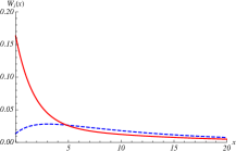
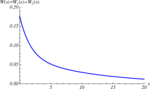
Figure 12: Plots of densities $W_{1}(x)$ (line) and $W_{2}(x)$ (dashes), on the left, and $W(x)=W_{1}(x)+W_{2}(x)$, on the right, for $\lambda_{1}^{*}=1$, $\mu_{1}^{*}=0.5$, $\lambda_{2}^{*}=1$, $\mu_{2}^{*}=2$, $\eta_{1}=0.1$, $\eta_{2}=0.08$, $\omega_{1}^{2}=1$ and $\omega_{2}^{2}=4$.

In the continuous approximation, by virtue of (65), from (70) one has:

$$\mathbb{P}(\mathscr{E}=i)\equiv M_{i}(0)=\int_{0}^{+\infty}W_{i}(x)\;dx={\eta_{3-i}\over\eta_{1}+\eta_{2}},\qquad i=1,2,$$ (72)

which provides the same result given in (20) for the discrete model.

Similarly to discrete case, we have that $\mathbb{P}(X<x|\mathscr{E}=1)$ and $\mathbb{P}(X<x|\mathscr{E}=2)$ are both generalized mixtures of two exponential distributions of means $1/\xi_{1}^{*}$ and $1/\xi_{2}^{*}$, respectively.

Making use of Proposition 6 and of (72), the conditional means immediately follow:

$$\mathbb{E}[X|\mathscr{E}=i]=\int_{0}^{+\infty}x\,{W_{i}(x)\over\mathbb{P}(\mathscr{E}=i)}\;dx={A_{i}^{*}\over\xi_{1}^{*}}+{1-A_{i}^{*}\over\xi_{2}^{*}},\qquad i=1,2.$$ (73)

Corollary 2

Under the assumptions of Proposition 6, for $x\in\mathbb{R}^{+}$ one obtains the steady-state density of the process $X$:

$$W(x)=W_{1}(x)+W_{2}(x)={\eta_{2}A_{1}^{*}+\eta_{1}A_{2}^{*}\over\eta_{1}+\eta_{2}}\,h_{1}(x)+\Bigl{[}1-{\eta_{2}A_{1}^{*}+\eta_{1}A_{2}^{*}\over\eta_{1}+\eta_{2}}\Bigr{]}\,h_{2}(x),$$ (74)

where $A_{1}^{*}$ and $A_{2}^{*}$ are provided in (68) and $h_{1}(x)$, $h_{2}(x)$ are exponential density with means $1/\xi_{1}^{*}$ and $1/\xi_{2}^{*}$, respectively.

Eq. (74) shows that also $W(x)$ is a generalized mixture of two exponential densities with means $1/\xi_{1}^{*}$ and $1/\xi_{2}^{*}$, respectively, so that

$$\mathbb{E}(X)={\eta_{2}A_{1}^{*}+\eta_{1}A_{2}^{*}\over\eta_{1}+\eta_{2}}{1\over\xi_{1}^{*}}+\Bigl{[}1-{\eta_{2}A_{1}^{*}+\eta_{1}A_{2}^{*}\over\eta_{1}+\eta_{2}}\Bigr{]}{1\over\xi_{2}^{*}}\cdot$$ (75)

Figure 12 shows the steady-state densities $W_{1}(x),W_{2}(x)$ (on the left) and $W(x)=W_{1}(x)+W_{2}(x)$ (on the right), obtained via Proposition 6 and Corollary 2, for $\lambda_{1}^{*}=1$, $\mu_{1}^{*}=0.5$, $\lambda_{2}^{*}=1$, $\mu_{2}^{*}=2$, $\eta_{1}=0.1$, $\eta_{2}=0.08$, $\omega_{1}^{2}=1$ and $\omega_{2}^{2}=4$. The roots of polynomial (63) can be evaluated by means of MATHEMATICA^®, so that $\xi_{1}^{*}=0.586811$, $\xi_{2}^{*}=0.0871$, $\xi_{3}^{*}=-1.17391$.

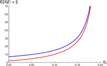
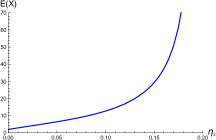
Figure 13: For $\lambda_{1}^{*}=1$, $\mu_{1}^{*}=0.5$, $\lambda_{2}^{*}=1$, $\mu_{2}^{*}=2$, $\eta_{1}=0.1$, $\omega_{1}^{2}=1$, $\omega_{2}^{2}=4$ and $0\leq\eta_{2}<0.2$, the conditional means $\mathbb{E}[X|\mathscr{E}=i]$, given in (73), are plotted on the left for $i=1$ (top) and $i=2$ (bottom), whereas the mean $\mathbb{E}(X)$ is plotted on the right.

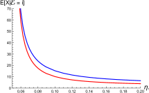
Figure 14: For $\lambda_{1}^{*}=1$, $\mu_{1}^{*}=0.5$, $\lambda_{2}^{*}=1$, $\mu_{2}^{*}=2$, $\eta_{2}=0.1$, $\omega_{1}^{2}=1$, $\omega_{2}^{2}=4$ and $\eta_{1}>0.05$, the conditional means $\mathbb{E}[X|\mathscr{E}=i]$, given in (73), are plotted on the left for $i=1$ (top) and $i=2$ (bottom), whereas the mean $\mathbb{E}(X)$ is plotted on the right.

Figure 13 gives, on the left, a plot of the conditional means, obtained in (73), for a suitable choice of the parameters, showing that $\mathbb{E}[X|\mathscr{E}=i]$ is increasing in $\eta_{2}$, for $i=1,2$. Furthermore, on the right of Figure 13 is plotted $\mathbb{E}(X)$ for the same choices of parameters. Similarly, in Figure 14 $\mathbb{E}[X|\mathscr{E}=i]$ (on the left) and $\mathbb{E}(X)$ (on the left) are plotted for the same choices of parameters, showing that they are decreasing in $\eta_{1}$.

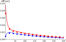
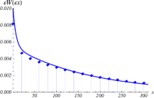
Figure 15: For $\lambda_{1}^{*}=1$, $\mu_{1}^{*}=0.5$, $\lambda_{2}^{*}=0.8$, $\mu_{2}^{*}=1.2$, $\eta_{1}=0.6$, $\eta_{2}=0.4$, $\omega_{1}^{2}=0.2$, $\omega_{2}^{2}=0.4$, on the left the functions $\epsilon\,W_{i}(\epsilon x)$ are compared with the probabilities $q_{n,i}$ for $i=1$ (square) and $i=2$ (circle), where $\lambda_{1},\mu_{1},\lambda_{2},\mu_{2}$ are given in (53) with $\epsilon=0.05$. On the right, for the same choices, the function $\epsilon\,W(\epsilon x)$ is compared with the probabilities $q_{n}$ (diamond).

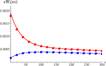
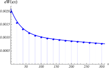
Figure 16: As in Figure 15, with $\epsilon=0.01$.

To show the validity tof the approximating procedure given in Section 4, in Figures 15(a) and 16(a), we compare the functions $\epsilon\,W_{i}(\epsilon x)$, where $W_{i}(x)$ is given in (67), with the probabilities $q_{n,i}$, given in (15), for $\epsilon=0.05$ and $\epsilon=0.01$, respectively. Furthermore, in Figures 15(b) and 16(b), we compare the functions $\epsilon\,W(\epsilon x)=\epsilon\,W_{1}(\epsilon x)+\epsilon\,W_{2}(\epsilon x)$, where $W(x)$ is given in (74), with the probabilities $q_{n}$, given in (22), for $\epsilon=0.05$ and $\epsilon=0.01$, respectively. The probabilities $q_{n,1}$ (square), the probabilities $q_{n,1}$ (circle) and the probabilities $q_{n}$ (diamond) are represented for $n=20\,k$ $(k=0,1,\ldots,15)$. According to (53), in Figures 15 we set $\lambda_{1}=60$, $\mu_{1}=50$, $\lambda_{2}=96$, $\mu_{2}=104$, whereas in Figures 16 one has $\lambda_{1}=1100$, $\mu_{1}=1050$, $\lambda_{2}=2080$, $\mu_{2}=2120$. From Figures 15 and 16, we note that the goodness of the diffusion approximation for the steady-state probabilities improves as $\epsilon$ decreases, due to an increase of traffic in the queueing system.

5 Analysis of the diffusion process for $\eta_{2}=0$

Let us now analyze the transient behaviour of the process ${\bf X}(t)=[X(t),\mathscr{E}(t)]$ in the case $\eta_{2}=0$, with the initial state specified in (56).

5.1 Probability densities

Similarly as in the discrete model, hereafter we express the probability densities (55) in terms of the transition densities $\widehat{r}^{(i)}(x,t|y)$ of two Wiener processes $\widehat{X}^{(i)}(t)$, characterized by drift $\beta_{i}=\lambda_{i}^{*}-\mu_{i}^{*}$ and infinitesimal variance $\omega_{i}^{2}$, $i=1,2$, restricted to $[0,+\infty)$, with $0$ reflecting boundary, given by (cf. [9])

$$\widehat{r}^{(i)}(x,t|y)={1\over\sqrt{2\pi\omega_{i}^{2}\,t}}\Biggl{[}\exp\biggl{\{}-{(x-y-\beta_{i}t)^{2}\over 2\,\omega_{i}^{2}\,t}\biggr{\}}$$

$$+\exp\biggl{\{}-{2\beta_{i}\,y\over\omega_{i}^{2}}\biggr{\}}\exp\biggl{\{}-{(x+y-\beta_{i}t)^{2}\over 2\,\omega_{i}^{2}\,t}\biggr{\}}\Biggr{]}$$

$$-{\beta_{i}\over\omega_{i}^{2}}\,\exp\biggl{\{}{2\,\beta_{i}\,x\over\omega_{i}^{2}}\biggr{\}}\,{\rm Erfc}\biggl{(}{x+y+\beta_{i}t\over\sqrt{2\,\omega_{i}^{2}\,t}}\biggr{)},\qquad x,y\in\mathbb{R}_{0}^{+},$$ (76)

where ${\rm Erfc}(x)=(2/\sqrt{\pi})\int_{x}^{+\infty}e^{-z^{2}}\,dz$ denotes the complementary error function.

Proposition 7

Let $\eta_{2}=0$. For all $t\geq 0$ and $y,x\in\mathbb{R}^{+}_{0}$, the probability densities (55) satisfy

$$f_{1}(x,t)=p\,e^{-\eta_{1}t}\,\widehat{r}^{(1)}(x,t\,|\,y),$$ (77)

$$f_{2}(x,t)=(1-p)\,\widehat{r}^{(2)}(x,t\,|\,y)$$

$$\hskip 14.22636pt+p\,\eta_{1}\int_{0}^{+\infty}dz\int_{0}^{t}\widehat{r}^{(1)}(z,\tau\,|\,y)\,e^{-\eta_{1}\tau}\,\widehat{r}^{(2)}(x,t-\tau\,|\,z)\;d\tau,$$ (78)

where $\widehat{r}^{(i)}(x,t|y)$ are provided in (76).

• It follows from (57), taking into account the boundary conditions (58) and the initial conditions (59). $\Box$

The probabilistic interpretation of (77) and (78) is similar to the discrete queueing model.

5.2 First-passage time problem

We consider the first-passage time through $(0,1)$ or $(0,2)$ states when $\eta_{2}=0$. To this purpose, we define a two-dimensional stochastic process $\{\widetilde{\bf X}(t)=[\widetilde{X}(t),\mathscr{E}(t)],t\geq 0\}$, obtained from ${\bf X}(t)$ by removing all the transitions from $(0,1)$ and $(0,2)$. We assume that $\widetilde{\bf X}(0)=(y,1)$ with probability $p$ and $\widetilde{\bf X}(0)=(y,2)$ with probability $1-p$, being $y\in\mathbb{R}^{+}$. Similarly to the discrete queueing model, only transitions from the first to the second environment are allowed. Hence, for $y\in\mathbb{R}^{+}$, denoting by

$$h_{i}(x,t|y)={d\over dt}\mathbb{P}\{\widetilde{X}(t)<x,\mathscr{E}(t)=i\},\qquad x\in\mathbb{R}^{+}_{0},\;i=1,2,\;t\geq 0$$ (79)

the transition density of the process $\widetilde{\bf X}(t)$, one has:

$${\partial h_{1}(x,t|y)\over\partial t}=-(\lambda_{1}^{*}-\mu_{1}^{*}){\partial h_{1}(x,t|y)\over\partial x}+{\omega_{1}^{2}\over 2}{\partial^{2}h_{1}(x,t|y)\over\partial x^{2}}-\eta_{1}h_{1}(x,t|y),$$

(80)

$${\partial h_{2}(x,t|y)\over\partial t}=-(\lambda_{2}^{*}-\mu_{2}^{*}){\partial h_{2}(x,t|y)\over\partial x}+{\omega_{2}^{2}\over 2}{\partial^{2}h_{2}(x,t|y)\over\partial x^{2}}+\eta_{1}h_{1}(x,t|y),$$

with the absorbing boundary conditions

$$\lim_{x\downarrow 0}h_{i}(x,t|y)=0,\qquad i=1,2$$ (81)

and the initial conditions

$$\lim_{t\downarrow 0}h_{1}(x,t|y)=p\,\delta(x-y),\quad\lim_{t\downarrow 0}h_{2}(x,t|y)=(1-p)\,\delta(x-y),\qquad 0\leq p\leq 1.$$ (82)

Hereafter we express the transition densities (79) in terms of the probability densities of the Wiener processes $\widehat{X}^{(i)}(t)$ in the presence of an absorbing boundary in the zero state for $x,y\in\mathbb{R}^{+}$, which is given by (cf. [9])

$$\widehat{\alpha}^{(i)}(x,t|y)={1\over\sqrt{2\,\pi\,\omega_{i}^{2}\,t}}\Biggl{[}\exp\biggl{\{}-{(x-y-\beta_{i}\,t)^{2}\over 2\,\omega_{i}^{2}\,t}\biggr{\}}$$

$$\hskip 28.45274pt-\exp\biggl{\{}-{2\beta_{i}\,y\over\omega_{i}^{2}}\biggr{\}}\exp\biggl{\{}-{(x+y-\beta_{i}\,t)^{2}\over 2\,\omega_{i}^{2}\,t}\biggr{\}}\Biggr{]},\qquad t>0.$$ (83)

Proposition 8

If $\eta_{2}=0$, for $y\in\mathbb{R}^{+}$, $x\in\mathbb{R}^{+}_{0}$ and $t>0$, the transition densities (79) can be expressed as:

$$h_{1}(x,t|y)=p\,e^{-\eta_{1}t}\,\widehat{\alpha}^{(1)}(x,t|y),$$ (84)

$$h_{2}(x,t|y)=(1-p)\,\widehat{\alpha}^{(2)}(x,t|y)$$

$$+\eta_{1}p\int_{0}^{\infty}dz\int_{0}^{t}e^{-\eta_{1}\tau}\,\widehat{\alpha}^{(1)}(z,\tau|y)\,\widehat{\alpha}^{(2)}(x,t-\tau|z)\;d\tau,$$ (85)

where $\widehat{\alpha}^{(i)}(x,t|y)$ are provided in (83).

• It follows from (80), taking into account the absorbing boundary conditions (81) and the initial conditions (82). $\Box$

We note that Eqs. (84) and (85) are similar to (40) and (41) for the discrete queueing model.

For $y\in\mathbb{R}^{+}$, let

$${\cal T}_{y}=\inf\{t>0:{\bf X}(t)=(0,1)\;{\rm or}\;{\bf X}(t)=(0,2)\},$$

be the FPT through zero for ${\bf X}(t)$ starting from $(y,1)$ with probability $p$ and from $(y,2)$ with probability $1-p$. We note that

$$\mathbb{P}({\cal T}_{y}<t)+\int_{0}^{+\infty}\bigl{[}h_{1}(x,t|y)+h_{2}(x,t|y)\bigr{]}\;dx=1.$$ (86)

Hereafter we focus on the FPT probability density

$$k(0,t|y)={d\over dt}\mathbb{P}({\cal T}_{y}<t),\qquad t>0,\;y\in\mathbb{R}^{+}.$$ (87)

Specifically, we express such density in terms of the FPT densities from state $y$ to state $x$ for the Wiener processes $\widehat{X}^{(i)}(t)$, given by

$$\widehat{g}^{(i)}(x,t|y)={y-x\over\sqrt{2\,\pi\,\omega_{i}^{2}\,t^{3}}}\exp\biggl{\{}-{(x-y-\beta_{i}\,t)^{2}\over 2\,\omega_{i}^{2}\,t}\biggr{\}},\qquad 0\leq x<y.$$ (88)

Proposition 9

If $\eta_{2}=0$ and $y\in\mathbb{R}^{+}$, for $t>0$ the FPT density (87) can be expressed as

$$k(0,t|y)=p\,e^{-\eta_{1}t}\,\widehat{g}^{(1)}(0,t|y)+(1-p)\,\widehat{g}^{(2)}(0,t|y)$$

$$+\eta_{1}p\int_{0}^{+\infty}dz\int_{0}^{t}e^{-\eta_{1}\tau}\,\widehat{\alpha}^{(1)}(z,\tau|y)\,\widehat{g}^{(2)}(0,t-\tau|z)\;d\tau,$$ (89)

where $g^{(i)}(0,t|y)$ are provided in (88).

• Making use of (80), (81) and (82), for $i=1,2$ one has

  $${d\over dt}\int_{0}^{+\infty}h_{i}(x,t|y)\;dx=-{\omega_{i}^{2}\over 2}\lim_{x\downarrow 0}{\partial\over\partial x}h_{i}(x,t|y)+(-1)^{i}\eta_{i}\int_{0}^{+\infty}h_{1}(x,t|y)\;dx,$$

  so that, from (86) and (87) it follows:

  $$k(0,t|y)={\omega_{1}^{2}\over 2}\lim_{x\downarrow 0}{\partial h_{1}(x,t|y)\over\partial x}+{\omega_{2}^{2}\over 2}\lim_{x\downarrow 0}{\partial h_{2}(x,t|y)\over\partial x}\cdot$$ (90)

  Recalling (83) and (88), for $y\in\mathbb{R}^{+}$ one has

  $$\lim_{x\downarrow 0}{\partial\over\partial x}\widehat{\alpha}^{(i)}(x,t|y)=2\,\omega_{i}^{2}\,\widehat{g}^{(i)}(0,t|y),\qquad i=1,2.$$

  Hence, (89) immediately follows from (84), (85) and (90). $\Box$

We note the high analogy in the FPT density $k(0,t|y)$, given in (89), with the FPT density $b_{j}(t)$, given in (45), of the discrete queueing model.

Let

$$K(s|y)={\cal L}[k(0,t|y)]=\int_{0}^{+\infty}e^{-s\,t}k(0,t|y)\;dt,\qquad s>0,y\in\mathbb{R}^{+}$$

be the Laplace transform of the FPT density $k(0,t|y)$.

Proposition 10

For $s>0$ and $y\in\mathbb{R}^{+}$, one has

$$K(s|y)=p\,e^{-y\zeta_{1}(s)}+(1-p)\,e^{-y\theta_{1}(s)}+{2\,\eta_{1}\,p\,\bigl{[}e^{-y\zeta_{1}(s)}-e^{-y\theta_{1}(s)}\bigr{]}\over\omega_{1}^{2}\bigl{[}\zeta_{1}(s)-\theta_{1}(s)\bigr{]}\,\bigl{[}\zeta_{2}(s)-\theta_{1}(s)\bigr{]}},$$ (91)

with

$$\zeta_{1}(s),\zeta_{2}(s)={\lambda_{1}^{*}-\mu_{1}^{*}\pm\sqrt{(\lambda_{1}^{*}-\mu_{1}^{*})^{2}+2\,\omega_{1}^{2}\,(s+\eta_{1})}\over\omega_{1}^{2}}$$ (92)

for $\zeta_{2}(s)<0<\zeta_{1}(s)$, and

$$\theta_{1}(s),\theta_{2}(s)={\lambda_{2}^{*}-\mu_{2}^{*}\pm\sqrt{(\lambda_{2}^{*}-\mu_{2}^{*})^{2}+2\,\omega_{2}^{2}\,s}\over\omega_{2}^{2}}$$ (93)

for $\theta_{2}(s)<0<\theta_{1}(s)$.

From (91) we determine the ultimate absorbing probability in $(0,1)$ or in $(0,2)$. Since $\eta_{2}=0$, if $\lambda_{2}^{*}\leq\mu_{2}^{*}$ then $\theta_{1}(0)=0$, so that ${\mathbb{P}}({\cal T}_{y}<\infty)=1$, whereas if $\lambda^{*}_{2}>\mu^{*}_{2}$, then we have $\theta_{1}(0)=2(\lambda_{2}^{*}-\mu_{2}^{*})/\omega_{2}^{2}$, so that for $y\in\mathbb{R}^{+}$ it results:

$$\mathbb{P}({\cal T}_{y}<+\infty)=\int_{0}^{+\infty}k(0,t|y)\;dt=p\,e^{-y\zeta_{1}(0)}+(1-p)\,\exp\Bigl{\{}-{2(\lambda_{2}^{*}-\mu_{2}^{*})y\over\omega_{2}^{2}}\Bigr{\}}$$

$$\hskip 62.59596pt+{2\,\eta_{1}\,p\,\Bigl{[}e^{-y\zeta_{1}(0)}-\exp\Bigl{\{}-{2(\lambda_{2}^{*}-\mu_{2}^{*})y\over\omega_{2}^{2}}\Bigr{\}}\Bigr{]}\over\omega_{1}^{2}\Bigl{[}\zeta_{1}(0)-{2(\lambda_{2}^{*}-\mu_{2}^{*})\over\omega_{2}^{2}}\Bigr{]}\,\Bigl{[}\zeta_{2}(0)-{2(\lambda_{2}^{*}-\mu_{2}^{*})\over\omega_{2}^{2}}\Bigr{]}},$$ (94)

with $\zeta_{1}(0),\zeta_{2}(0)$ given in (92) for $s=0$.

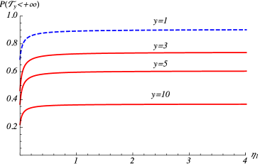
(a) $\lambda_{1}^{*}=1.0,\mu_{1}^{*}=0.5$

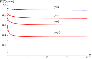
(b) $\lambda_{1}^{*}=0.5,\mu_{1}^{*}=1.0$

Figure 17: Plots of FPT probabilities $\mathbb{P}({\cal T}_{y}<+\infty)$ as function of $\eta_{1}$ for $\eta_{2}=0$, $\lambda^{*}_{2}=1.2$, $\mu^{*}_{2}=1.0$, $\omega_{1}^{2}=1$, $\omega_{2}^{2}=4$ and $p=0.4$.

For $\lambda_{2}^{*}>\mu_{2}^{*}$, in Figure 17 we plot $\mathbb{P}({\cal T}_{y}<+\infty)$, given in (94), as function of $\eta_{1}$ for $y=1,3,5,10$.

When $\lambda_{2}^{*}<\mu_{2}^{*}$, $\eta_{1}>0$ and $y\in\mathbb{R^{+}}$, from (91) we obtain the FPT mean

$$\mathbb{E}({\cal T}_{y})={y\over\mu_{2}^{*}-\lambda_{2}^{*}}+{p\over\eta_{1}}\,\Bigl{(}1-{\mu_{1}^{*}-\lambda_{1}^{*}\over\mu_{2}^{*}-\lambda_{2}^{*}}\Bigr{)}\Bigl{(}1-e^{-y\zeta_{1}(0)}\Bigr{)}.$$ (95)

Finally, in Figure 18 we plot the mean (95) as function of $\eta_{1}$; since $\lambda_{2}^{*}<\mu_{2}^{*}$, the first passage through zero state is a certain event.

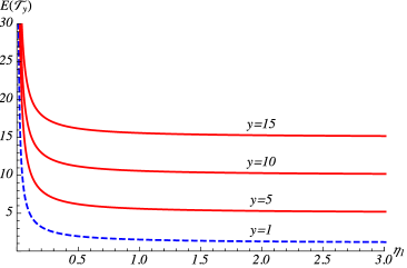
(a) $\lambda_{1}^{*}=1.0,\mu_{1}^{*}=0.5$

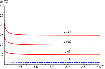
(b) $\lambda_{1}^{*}=0.5,\mu_{1}^{*}=1.0$

Figure 18: Plots of FPT mean $\mathbb{E}({\cal T}_{y})$ as function of $\eta_{1}$ for $\eta_{2}=0$, $\lambda^{*}_{2}=1.0$, $\mu^{*}_{2}=2.0$, $\omega_{1}^{2}=1$, $\omega_{2}^{2}=4$ and $p=0.4$.

Concluding remarks

In this paper we considered a an $M/M/1$ queue whose behavior fluctuates randomly between two different environments according to a two-state continuous-time Markov chain.

We first get the steady-state distribution of the system, which is expressed via a generalized mixture of two geometric distributions. A remarkable result is that the system admits of a steady-state distribution even if one of the alternating environments does not possess a steady state. Hence, the switching between the environments can be used to stabilize a non stationary $M/M/1$ queue by means of the random alternation with a similar queue characterized by steady state.

Moreover, attention has been given to the transient distribution of the alternating queue, which can be expressed in a series form involving the queue-length distribution in absence of switching. A similar result is obtained also for the first-passage-time density through the zero state, in order to investigate the busy period.

The second part of the paper has been centered on a heavy-traffic approximation of the queue-length process, that leads to an alternating Wiener process restricted by a reflecting boundary at zero. The analysis of the approximating process has been devoted to the steady-state density, which is expressed as a generalized mixture of two exponential densities. Moreover, we determined the transition density when only one type of switch is allowed. Such density can be decomposed in an integral form involving the expressions of the Wiener process in the presence of a reflecting boundary at zero. Finally, we analyzed the first-passage-time density through the zero state, which gives a suitable approximation of the busy period density.

References

- [1] Abate, J., Kijima, M., Whitt, W. (1991) Decompositions of the transition function. Queueing Syst. 9, 323–336.
- [2] Arunachalam, V., Gupta, V., Dharmaraja, S. (2010) A fluid queue modulated by two independent birth-death processes. Comput. Math. Appl. 60, 2433–2444.
- [3] Avissar, O., Yechiali, U. (2012) Polling systems with two alternating weary servers. Semantic Scholar.
- [4] Bezák, V. (1992) A modification of the Wiener process due to a Poisson random train of diffusion-enhancing pulses. J. Phys. A 25, 6027–6041.
- [5] Boxma, O.J., Kurkova, I.A. (2000) The queue in a heavy-tailed random environment. Stat. Neerl. 54, 221–236.
- [6] Boxma, O.J., Kurkova, I.A. (2001) The queue with two service speeds. Adv. Appl. Prob. 33, 520–540.
- [7] Boxma, O.J., Schlegel, S., Yechiali, U. (2002) Two-queue polling models with a patient server. Ann. Oper. Res. 112, 101–121.
- [8] Burman, D.Y., Smith, D.R. (1986) An asymptotic analysis of a queueing system with Markov-modulated arrivals. Oper. Research 34, 105–119.
- [9] Cox, D.R., Miller, H.D. (1970) The Theory of Stochastic Processes. Methuen, London.
- [10] D’Auria, B. (2014) queue with on-off service speeds. J. Math. Sci. 196, 37–42.
- [11] Dharmaraja, S., Di Crescenzo, A., Giorno, V., Nobile, A.G. (2015) A continuous-time Ehrenfest model with catastrophes and its jump-diffusion approximation. J. Stat. Phys. 161, 326–345.
- [12] Di Crescenzo, A., Di Nardo, E., Ricciardi, L.M. (2005) Simulation of first-passage times for alternating Brownian motions. Methodol. Comput. Appl. Probab. 7, 161–181.
- [13] Di Crescenzo, A., Giorno, V., Krishna Kumar, B., Nobile, A.G. (2012) A double-ended queue with catastrophes and repairs, and a jump-diffusion approximation. Methodol. Comput. Appl. Probab. 14, 937–954.
- [14] Di Crescenzo, A., Giorno, V., Nobile, A.G. (2016) Constructing transient birth-death processes by means of suitable transformations. Appl. Math. Comput. 281, 152–171.
- [15] Di Crescenzo, A., Giorno, V., Nobile, A.G., Ricciardi, L.M. (2003) On the queue with catastrophes and its continuous approximation. Queueing Syst. 43, 329–347.
- [16] Di Crescenzo, A., Nobile, A.G. (1995) Diffusion approximation to a queueing system with time-dependent arrival and service rates. Queueing Syst. 19, 41–62.
- [17] Di Crescenzo, A., Zacks, S. (2015) Probability law and flow function of Brownian motion driven by a generalized telegraph process. Methodol. Comput. Appl. Probab. 17, 761–780.
- [18] Economou, A., Manou, A. (2016) Strategic behavior in an observable fluid queue with an alternating service process. European J. Oper. Res. 254, 148–160.
- [19] Eliazar, I., Fibich, G., Yechiali, U. (2002) A communication multiplexer problem: two alternating queues with dependent randomly-timed gated regime. Queueing Syst. 42, 325–353.
- [20] Erdélyi, A., Magnus, W., Oberhettinger, F., Tricomi, F.G. (1954) Tables of integral transforms. Vol. I. Based, in part, on notes left by Bateman, H. McGraw-Hill, New York.
- [21] Giorno, V., Nobile, A.G., Pirozzi, E. (2018) A state-dependent queueing system with asymptotic logarithmic distribution. J. Math. Anal. Appl. 458, 949–966.
- [22] Giorno, V., Nobile, A.G., Ricciardi, L.M. (1987) On some time-nonhomogeneous diffusion approximations to queueing systems. Adv. Appl. Prob. 19, 974–994.
- [23] Giorno, V., Nobile, A.G., Spina, S. (2014) On some time non-homogeneous queueing systems with catastrophes. Appl. Math. Comput. 245, 220–234.
- [24] Gradshteyn, I.S., Ryzhik, I.M. (2007) Tables of Integrals, Series and Products, 7th ed. Academic Press, Amsterdam.
- [25] Jiang, T., Liu, L., Li, J. (2015) Analysis of the queue in multi-phase random environment with disasters. J. Math. Anal. Appl. 430, 857–873.
- [26] Huang, L., Lee, T.T. (2013) Generalized Pollaczek-Khinchin formula for Markov channels. IEEE Trans. Commun. 61, 3530–3540.
- [27] Kao, E.P.C., Lin, C. (1989) The queue with randomly varying arrival and service rates: a phase substitution solution. Management Sci. 35, 561–570.
- [28] Kim, B.K., Lee, D.H. (2014) The M/G/1 queue with disasters and working breakdowns. Appl. Math. Model. 38, 1788–1798.
- [29] Krishna Kumar, B., Pavai Madheswari, S. (2005) Transient analysis of an queue subject to catastrophes and server failures. Stoch. Anal. Appl. 23, 329–340.
- [30] Liu, Z., Yu, S. (2016) The M/M/C queueing system in a random environment. J. Math. Anal. Appl. 436, 556–567.
- [31] Lu, F.V., Serfozo, R.F. (1984) queueing decision processes with monotone hysteretic optimal policies. Oper. Research 32, 1116–1132.
- [32] Mandelbaum, A., Massey, W.A. (1995) Strong approximations for time-dependent queues. Math. Oper. Res. 20, 33–64.
- [33] Medhi, J. (2003) Stochastic Models in Queueing Theory. Second edition. Academic Press, Amsterdam.
- [34] Navarro, J. (2016) Stochastic comparisons of generalized mixtures and coherent systems. TEST 25, 150–169.
- [35] Neuts, M.F. (1978) The queue with randomly varying arrival and service rates. Opsearch 15, 139–157.
- [36] Pang, G., Zhou, Y. (2016) queues with renewal alternating interruptions. Adv. Appl. Prob. 48, 812–831.
- [37] Paz, N., Yechiali, U. (2014) An queue in random environment with disasters. Asia-Pacific J. Oper. Res. 31, 1450016.
- [38] Perel, E., Yechiali, U. (2017) Two-queue polling systems with switching policy based on the queue that is not being served. Stoch. Models, 1–21.
- [39] Yechiali, U., Naor, P. (1971) Queuing problems with heterogeneous arrivals and service. Oper. Res., 19, 722–734.
- [40] Zhang, J., Coyle, E.J., Jr. (1991) The transient solution of time-dependent queues. IEEE Trans. Inform. Theory 37, 1690–1696.