A continuous-time Ehrenfest model with catastrophes and its jump-diffusion approximation

Abstract

We consider a continuous-time Ehrenfest model defined over the integers from $-N$ to $N$, and subject to catastrophes occurring at constant rate. The effect of each catastrophe instantaneously resets the process to state 0. We investigate both the transient and steady-state probabilities of the above model. Further, the first passage time through state 0 is discussed. We perform a jump-diffusion approximation of the above model, which leads to the Ornstein-Uhlenbeck process with catastrophes. The underlying jump-diffusion process is finally studied, with special attention to the symmetric case arising when the Ehrenfest model has equal upward and downward transition rates.

Keywords: Transient probabilities, Steady-state probabilities, First passage time, Ornstein-Uhlenbeck process.
Mathematics Subject Classification: 60J80; 60J27; 60J60.

1 Introduction

The Ehrenfest model describes a simple diffusion process as a Markov chain, where molecules of a gas are in a container divided into two equal parts by a permeable membrane and diffuse at random according to the number of molecules in a single part. This model, that was originally proposed to explain the second law of thermodynamics on the macroscopic scale, deserves large interest in physics and in applied sciences, stimulating indeed various investigations due to its flexibility and wide applicability. Among the recent contributions related to the continuous-time version of this model we recall Balaji et al. [1], where the status of the system is studied in detail after a certain number of steps, by considering three phases depending on the number of molecules. We also mention Flegg et al. [18], where a theory of the degradation and thermal fragmentation kinetics of polymerlike systems is analysed by means of a first passage time problem through state zero. Hauert et al. [23] propose a generalization of the original model by including the possibility that a single state changes with probability $p$.

Modified Ehrenfest models are worthy of interest also in mathematical finance, for instance to describe returns in stock index prices under the effect of large jumps (see Takahashi [38]). Continuous-time stochastic systems are often investigated under the presence of jumps (describing the effect of total catastrophes) in order to capture the presence of more realistic conditions.

Along this line our purpose is to investigate an Ehrenfest model subject to catastrophes, as well as its jump-diffusion approximation. The reference model is a continuous-time skip-free Markov chain superimposed by randomly occurring jumps. The literature in this field is quite large. By restricting our attention mainly to birth-death processes subject to catastrophes, as suitable examples we refer to the papers by Brockwell [2], [3], Cairns and Pollett [4] and Pollett et al. [35] (where necessary and sufficient conditions are given such a birth-death-catastrophe process reaches the extinction), Chao and Zheng [5], Kyriakidis [32], Renshaw and Chen [36] (for the study of the transient and equilibrium behaviors of the immigration-birth-death process with catastrophes), Kyriakidis [29], [30], [31], Zeifman et al. [40], Van Doorn and Zeifman [39], Giorno and Nobile [19], Giorno et al. [21] and Di Crescenzo et al. [13] (for the analysis of various types of birth-death processes under the influence of catastrophes), Pakes [33], Chen et al. [8] and Economou and Fakinos [14], [15] (for the determination of various distributions and other quantities of interest for continuous-time Markov chains subject to catastrophes), Chen and Renshaw [6] and [7], and Krishna Kumar et al. [27] and [28] (for the analysis of Markovian queueing systems in the presence of mass annihilations).

It is worth noting that there has been recently some interest in the statistical physics literature on stochastic processes subject to catastrophes, but under the different name of ‘processes with stochastic reset’. In this field attention has been given to simple diffusions where a particle stochastically resets to its initial position at a constant rate. We recall the contributions by Evans and Majumdar on the Brownian motion with reset, where the mean time to find a stationary target by a diffusive searcher is investigated [16], and where a problem of optimal resetting is addressed [17]. More recent results in the area of stochastic processes with resetting are related to general diffusions (see Pal [34]), and one-dimensional Lévy flights, also known as intermittent random walks (cf. Kusmierz et al. [26]).

Many discrete stochastic systems are often investigated under suitable limiting conditions leading to diffusion processes. The case of the discrete-time Ehrenfest model was first treated in Section 4 of Kac [25], where the Ornstein-Uhlenbeck process was employed. With reference to models subject to catastrophes we recall the jump-diffusion approximations to the M/M/1 queue and to a double-ended queue both based on the Wiener process (see Di Crescenzo et al.  [11], [12]). Other jump-diffusion models involving the Ornstein-Uhlenbeck process and other processes have been investigated in di Cesare et al. [9], and Giorno et al. [20]. In this paper we perform a suitable scaling limit on the continuous-time Ehrenfest model that leads to a suitable jump-diffusion process of the Ornstein-Uhlenbeck type.

The appropriately normalized Ehrenfest model converges weakly to a limiting diffusion process that is the Ornstein-Uhlenbeck process, even in the multidimensional case (see Iglehart [24]). In this paper we purpose to show that the Ehrenfest model subject to catastrophes in the limit converges to a jump-diffusion process, which is again of the Ornstein-Uhlenbeck type. The necessity of resorting to a continuous approximation is due to the fact that the expressions of the transition probabilities and of the stationary distribution of the Ehrenfest model with catastrophes are computationally intractable for large values of the involved parameters.

This is the plan of the paper. In Section 2, we introduce the continuous-time stochastic process describing the Ehrenfest model defined on the integers from $-N$ to $N$. The model includes the occurence of catastrophes arriving according to the exponential distribution with constant rate, whose effect is to set the state of the system equal to 0. We relate the relevant functions of the process to those of the birth-death process obtained by removing the possibility of catastrophes. This allows to determine the transient probabilities, the mean and the second order moment. In Section 3, we propose a jump-diffusion approximation of the Ehrenfest model with catastrophes. We obtain the Fokker-Planck equation for the approximating jump-diffusion process. This is defined on the set of real numbers, and possesses linear drift and constant infinitesimal variance. In particular, we are able to obtain the mean and the second order moment of the process in the transient phase. The steady-state density is also evaluated, expressed in closed form in terms of the parabolic cylinder function. The first passage time problem through state 0 is also faced. We obtain the explicit expression of the first passage time density and of its mean. In conclusion, special attention is devoted to the jump-diffusion approximation in the special case in which the Ehrenfest model has equal upward and downward transition rates. In this case both the discrete model and the jump-diffusion approximating process exhibit certain suitable symmetries.

We point out that various computational results shown in this paper have been obtained by use of Mathematica ®. Note that throughout the paper we denote by $E_{j}[Y(t)]$ and $V_{j}[Y(t)]$ the mean and the variance, respectively, of any stochastic process $Y(t)$ conditional on $Y(0)=j$. Moreover, we denote the rising factorial as $(\alpha)_{n}=\alpha(\alpha+1)\cdots(\alpha+n-1)$, for $n\geq 1$, with $(\alpha)_{0}=1$.

2 A stochastic model with catastrophes

We consider a system subject to catastrophes, described by a stationary Markov chain $\{M(t),t\geq 0\}$ defined on the state-space $S=\{-N,-N+1,\ldots,-1,0,1,\ldots,N\}$, with $N$ a positive integer. We suppose that the catastrophes occur according to a Poisson process with intensity $\xi$. Denoting by

$$r(k,n)=\lim_{h\to 0^{+}}\frac{1}{h}P\{M(t+h)=n\,|\,M(t)=k\},\qquad k,n\in S$$

the transition rate function of $M(t)$, we assume that the allowed transitions occur according to the following scheme:

$$r(-1,0)=\lambda(N+1)+\xi,\qquad r(n,n+1)=\lambda(N-n),\quad\forall\;\;n\in S\setminus\{-1\};$$ (1)

$$r(1,0)=\mu(N+1)+\xi,\qquad r(n,n-1)=\mu(N+n),\quad\forall\;\;n\in S\setminus\{1\};$$ (2)

$$r(n,0)=\xi,\quad n\in S\setminus\{0\},$$ (3)

with $\lambda,\mu,\xi>0$. Hence, $\{M(t),t\geq 0\}$ is a time-homogeneous continuous-time Markov chain with transition rates (1), (2) and (3), and is defined on the state-space $S$, where $S$ is an irreducible class. Eq. (3) defines the catastrophe rate, the effect of each catastrophe being the instantaneous transition to the state $0$ (cf. Figure 1).

It is worth pointing out that in the absence of catastrophes and in the symmetric case $\lambda=\mu$, the imbedded random walk that describes the state changes of $M(t)$ identifies with the stochastic process studied in Section 4 of Kac [25]. Moreover, $M(t)$ can also be viewed as a suitable modification of the Prendiville process (see Zheng [41] and references therein).

Due to (1), (2) and (3), for all $j,n\in S$ and $t\geq 0$ the transition probabilities

$$p_{j,n}(t)=P\{M(t)=n\mid M(0)=j\}\qquad(j,n\in S)$$

satisfy the following differential-difference equations:

$$\left\{\begin{array}[]{l}\frac{d}{dt}p_{j,0}(t)=-[N(\lambda+\mu)+\xi]p_{j,0}(t)+(N+1)\lambda p_{j,-1}(t)+(N+1)\mu p_{j,1}(t)+\xi,\\[5.69046pt] \frac{d}{dt}p_{j,n}(t)=-[(N-n)\lambda+(N+n)\mu+\xi]p_{j,n}(t)+(N-n+1)\lambda p_{j,n-1}(t)\\[2.84544pt] \hskip 56.9055pt+(N+n+1)\mu p_{j,n+1}(t),\hskip 85.35826ptn=\pm 1,\pm 2,\ldots,\pm(N-1),\\[5.69046pt] \frac{d}{dt}p_{j,-N}(t)=-(2N\lambda+\xi)p_{j,-N}(t)+\mu p_{j,-N+1}(t),\\[5.69046pt] \frac{d}{dt}p_{j,N}(t)=-(2N\mu+\xi)p_{j,N}(t)+\lambda p_{j,N-1}(t).\end{array}\right.$$ (4)

The initial condition for system (4) is expressed in terms of the Kronecker’s delta:

$$p_{j,n}(0)=\delta_{j,n}=\left\{\begin{array}[]{ll}1,&n=j\\ 0,&\mbox{otherwise}.\end{array}\right.$$ (5)

Figure 1: The state diagram of the process $M(t)$.

It is customary to study a Markov process subject to catastrophes by referring to the basic process (i.e. in absence of catastrophes). To this aim, we denote by $\{\widetilde{M}(t),t\geq 0\}$ the stochastic process corresponding to $\{M(t),t\geq 0\}$ when $\xi\to 0^{+}$. Hence, $\widetilde{M}(t)$ constitutes a continuous-time skip-free Markov chain, i.e. a time-homogeneous birth-death process without catastrophes, defined on the state space $S$, and obtained from $M(t)$ by removing the possibility of catastrophes. For all $t\geq 0$ we introduce the transition probabilities

$$\widetilde{p}_{j,n}(t)=P\{\widetilde{M}(t)=n\mid\widetilde{M}(0)=j\},\qquad j,n\in S,$$

with the initial condition

$$\widetilde{p}_{j,n}(0)=\delta_{j,n}.$$

Conditioning on the age of the catastrophe process it is not hard to see that the transition probabilities $p_{j,n}(t)$ and $\widetilde{p}_{j,n}(t)$ are related by the following equation (cf., for instance, Kyriakidis [29], Pakes [33] or Renshaw and Chen [36]):

$$p_{j,n}(t)=e^{-\xi t}\widetilde{p}_{j,n}(t)+\xi\int_{0}^{t}e^{-\xi\tau}\widetilde{p}_{0,n}(\tau)d\tau,\qquad j,n\in S,\;\;t\geq 0.$$ (6)

Hence, due to (6) the $k$-th conditional moment of $M(t)$ can be related to that of $\widetilde{M}(t)$ for $k=1,2,\ldots$, since

$$E_{j}[M^{k}(t)]=e^{-\xi t}E_{j}[\widetilde{M}^{k}(t)]+\xi\int_{0}^{t}e^{-\xi\tau}E_{0}[\widetilde{M}^{k}(\tau)]d\tau,\qquad j\in S,\;\;t\geq 0.$$ (7)

Moreover, let

$${\cal T}_{j}=\inf\{t\geq 0:M(t)=0\},\qquad M(0)=j,\quad j\in S\setminus\{0\}$$

be the first-passage time of $M(t)$ through state 0, and let $g_{j,0}(t)$ denote the corresponding density. We have (see, for instance, [33] or [13]):

$$g_{j,0}(t)=e^{-\xi t}\widetilde{g}_{j,0}(t)+\xi\,e^{-\xi t}\left[1-\int_{0}^{t}\widetilde{g}_{j,0}(\tau)\,d\tau\right],\qquad j\in S\setminus\{0\},\;\;t\geq 0,$$ (8)

where $\widetilde{g}_{j,0}(t)$ is the first-passage-time density of $\widetilde{M}(t)$ through state 0 when $\widetilde{M}(0)=j$.

2.1 The discrete process in absence of catastrophes

Aiming to study $M(t)$ by means of relations (6), (7) and (8) we now recall some useful results on process $\{\widetilde{M}(t),t\geq 0\}$. We first notice that $\widetilde{M}(t)$ can be expressed as (similarly as in Zheng [41]):

$$\widetilde{M}(t)\stackrel{{\scriptstyle d}}{{=}}\widetilde{M}_{1}(t)+\widetilde{M}_{2}(t)-N,\qquad t\geq 0,$$ (9)

where, for any fixed $t\geq 0$, $\widetilde{M}_{1}(t)$ and $\widetilde{M}_{2}(t)$ are independent binomial random variables such that, under condition $\widetilde{M}(0)=j$,

$$\widetilde{M}_{1}(t)\sim{\cal B}in\left(N+j,b_{1}(t)\right),\qquad\widetilde{M}_{2}(t)\sim{\cal B}in\left(N-j,b_{2}(t)\right),$$ (10)

with

$$b_{1}(t)=\frac{\lambda+\mu e^{-(\lambda+\mu)t}}{\lambda+\mu},\qquad b_{2}(t)=\frac{\lambda}{\lambda+\mu}\left(1-e^{-(\lambda+\mu)t}\right),\qquad t\geq 0,$$ (11)

and where ‘$\stackrel{{\scriptstyle d}}{{=}}$’ means equality in distribution. This allows to obtain the transition probabilities for $j,n\in S$ and $t\geq 0$:

$$\widetilde{p}_{j,n}(t)\!\! = \!\!\sum_{i=\max\{0,j+n\}}^{\min\{N+n,N+j\}}\binom{N+j}{i}\binom{N-j}{N+n-i}[b_{1}(t)]^{i}[1-b_{1}(t)]^{N+j-i}[b_{2}(t)]^{N+n-i}[1-b_{2}(t)]^{i-j-n}$$

$$= \!\!\frac{\mu^{N+j}}{(\lambda+\mu)^{2N}}\left[1-e^{-(\lambda+\mu)t}\right]^{N+j}\left[\mu+\lambda e^{-(\lambda+\mu)t}\right]^{N-j}$$

$$\times \!\!\sum_{i=\max\{0,j+n\}}^{\min\{N+n,N+j\}}\binom{N+j}{i}\binom{N-j}{N+n-i}\left[\frac{\lambda+\mu e^{-(\lambda+\mu)t}}{\mu\left(1-e^{-(\lambda+\mu)t}\right)}\right]^{i}\left[\frac{\lambda\left(1-e^{-(\lambda+\mu)t}\right)}{\mu+\lambda e^{-(\lambda+\mu)t}}\right]^{N+n-i}.$$

Note that from (LABEL:prob_2N) the following symmetry property holds, with obvious notation:

$$\widetilde{p}_{j,n}(t;\lambda,\mu)=\widetilde{p}_{-j,-n}(t;\mu,\lambda),\qquad j,n\in S,\;\;t\geq 0.$$ (13)

We now provide the conditional mean and variance of $\{\widetilde{M}(t),t\geq 0\}$, obtained from Eqs. (9), (10) and (11):

$$E_{j}[\widetilde{M}(t)]\!\! = \!\!je^{-(\lambda+\mu)t}+\frac{(\lambda-\mu)N}{\lambda+\mu}\left(1-e^{-(\lambda+\mu)t}\right),$$ (14)

$$V_{j}[\widetilde{M}(t)]\!\! = \!\!\frac{1-e^{-(\lambda+\mu)t}}{(\lambda+\mu)^{2}}\Big{\{}(N+j)\mu\left(\lambda+\mu e^{-(\lambda+\mu)t}\right)+(N-j)\lambda\left(\mu+\lambda e^{-(\lambda+\mu)t}\right)\Big{\}}.$$ (15)

Let us now denote by $\widetilde{M}$ the random variable that describes the stationary state of the process. By letting $t\rightarrow\infty$ in Eq. (LABEL:prob_2N), we have

$$\widetilde{q}_{n}:=P(\widetilde{M}=n)=\lim_{t\to+\infty}\widetilde{p}_{j,n}(t)=\binom{2N}{N-n}(1+\rho)^{-2N}\rho^{n+N},\qquad n\in S,$$ (16)

where we have set $\rho=\lambda/\mu$. Hence, from (16) it follows

$$E[\widetilde{M}]=\frac{N(\rho-1)}{1+\rho},\qquad Var[\widetilde{M}]=\frac{2N\rho}{(1+\rho)^{2}}.$$

Finally, we recall that when $\lambda=\mu$ relation (13) allows to obtain a closed-form expression for the first-passage-time density through state $0$. Indeed, if $\lambda=\mu$ we have (cf. Theorem 4.3 of [10])

$$\widetilde{g}_{j,0}(t)=\mu(N+1)\,{\rm sgn}(j)[\widetilde{p}_{j,1}(t)-\widetilde{p}_{j,-1}(t)],\qquad j\in S\setminus\{0\},\;\;t\geq 0,$$ (17)

where ${\rm sgn}(j)=1$ if $j>0$ and ${\rm sgn}(j)=-1$ if $j<0$.

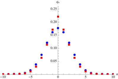
(a) $\lambda=0.6,\mu=0.6,\xi=0.5$

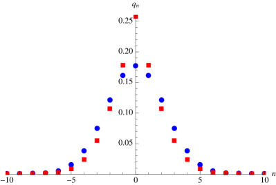
(b) $\lambda=0.6,\mu=0.6,\xi=1.0$

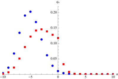
(c) $\lambda=0.2,\mu=0.6,\xi=0.5$

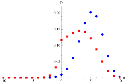
(d) $\lambda=0.6,\mu=0.2,\xi=0.5$

Figure 2: The steady-state probabilities $q_{n}$ (square) and $\widetilde{q}_{n}$ (circle) for $N=10$.

2.2 The discrete process with catastrophes

In this section we study the process $M(t)$. We first determine the stationary distribution, namely

$$q_{n}:=\lim_{t\to+\infty}p_{j,n}(t),\qquad n\in S.$$

Proposition 2.1

For all $n\in S$ we have

$$q_{n}\!\! = \!\!\xi\frac{\lambda^{N+n}\mu^{N-n}}{(\lambda+\mu)^{2N+1}}\sum_{i=\max\{0,n\}}^{\min\{N,N+n\}}\binom{N}{i}\binom{N}{N+n-i}\,B\left(2N+n-2i+1,\frac{\xi}{\lambda+\mu}\right)$$ (18)

$$\times \!\!F_{1}\left(\frac{\xi}{\lambda+\mu},-i,n-i,\frac{\xi}{\lambda+\mu}+2N+n-2i+1;-\frac{\mu}{\lambda},-\frac{\lambda}{\mu}\right),$$

where $B(x,y)={\Gamma(x)\Gamma(y)}/{\Gamma(x+y)}$ is the beta function, and

$$F_{1}\left(\alpha,\beta,\gamma,\delta;x,y\right)=\sum_{m=0}^{+\infty}\sum_{n=0}^{+\infty}\frac{(\alpha)_{m+n}(\beta)_{m}(\gamma)_{n}}{(\delta)_{m+n}}\,\frac{x^{m}}{m!}\,\frac{y^{n}}{n!}\qquad(|x|<1,\;|y|<1)$$

is the hypergeometric function of two variables (see, for instance, [22] p. 1018, n. 9.180.1).

• From (6), in the limit as $t\to+\infty$, one has $q_{n}=\xi\int_{0}^{+\infty}e^{-\xi\tau}\widetilde{p}_{0,n}(\tau)d\tau$, $n\in S$. Hence, making use of (LABEL:prob_2N) after some calculations we obtain

  $$q_{n}\!\! = \!\!\xi\frac{\lambda^{N+n}\mu^{N-n}}{(\lambda+\mu)^{2N+1}}\sum_{i=\max\{0,n\}}^{\min\{N,N+n\}}\binom{N}{i}\binom{N}{N+n-i}$$

  $$\times \!\!\int_{0}^{1}y^{-1+\xi/(\lambda+\mu)}(1-y)^{2N+n-2i}\left(1+\frac{\mu}{\lambda}\,y\right)^{i}\left(1+\frac{\lambda}{\mu}\,y\right)^{i-n}dy.$$

  Recalling that (cf. [22], p. 318, n. 3.211)

  $$\int_{0}^{1}x^{a-1}(1-x)^{b-1}(1-ux)^{-\rho}(1-vx)^{-\sigma}dx=B(b,a)\,F_{1}(a,\rho,\sigma,a+b;u,v)\qquad(a>0,\;b>0),$$

  we finally have (18). $\hfill\Box$

We note that from Eqs. (16) and (18) one can prove that $\lim_{\xi\to 0^{+}}q_{n}=\widetilde{q}_{n}$, for $n\in S$. In Figure 2 we provide some plots of $q_{n}$ and $\widetilde{q}_{n}$ for various choices of $\lambda$, $\mu$ and $\xi$. Specifically, cases (a) and (b) show instances in which $\lambda=\mu$, and thus $q_{n}=q_{-n}$ for all $n\in S$. Clearly, when $\xi$ increases then $q_{n}$ is more peaked in $n=0$. Cases (c) and (d) show symmetric plots, due to relation $q_{n}(\lambda,\mu)=q_{-n}(\mu,\lambda)$, $n\in S$, with obvious notation.

In the following proposition we express the transition probabilities of $M(t)$ as the sum of the stationary distribution obtained in Proposition 2.1 and a time-varying term that vanishes as $t\to+\infty$.

Proposition 2.2

For all $j,n\in S$ and $t\geq 0$ we have

$$p_{j,n}(t)\!\! = \!\!q_{n}+\widetilde{p}_{j,n}(t)e^{-\xi t}-\xi\frac{\lambda^{N+n}\mu^{N-n}}{(\lambda+\mu)^{2N}}e^{-\xi t}\sum_{i=\max\{0,n\}}^{\min\{N,N+n\}}\binom{N}{i}\binom{N}{N+n-i}$$

$$\times \!\!\sum_{h=0}^{i}\binom{i}{h}\left[\frac{\mu}{\lambda}\,e^{-(\lambda+\mu)t}\right]^{h}\sum_{k=0}^{i-n}\binom{i-n}{k}\left[\frac{\lambda}{\mu}\,e^{-(\lambda+\mu)t}\right]^{k}$$

$$\times \!\!\frac{1}{\xi+(h+k)(\lambda+\mu)}\,F\left(\frac{\xi}{\lambda+\mu}+h+k,2(i-N)-n;\frac{\xi}{\lambda+\mu}+h+k+1;e^{-(\lambda+\mu)t}\right),$$

where $q_{n}$ and $\widetilde{p}_{j,n}(t)$ are given respectively in (18) and (LABEL:prob_2N), and where (cf. [22], p. 1005, n. 9.100)

$$F(a,b;c;z)=\sum_{n=0}^{+\infty}\frac{(a)_{n}(b)_{n}}{(c)_{n}}\,\frac{z^{n}}{n!}$$

is the Gauss hypergeometric function.

• In order to obtain the transition probabilities of $M(t)$ we evaluate the integral in the right-hand-side of (6). Due to (LABEL:prob_2N) and after some calculations, for $t\geq 0$ and $n\in S$ we have

  $$\int_{0}^{t}e^{-\xi\tau}\widetilde{p}_{0,n}(\tau)d\tau=\frac{\lambda^{N+n}\mu^{N}}{(\lambda+\mu)^{2N}}\sum_{i=\max\{0,n\}}^{\min\{N,N+n\}}\binom{N}{i}\binom{N}{N+n-i}(\lambda\mu)^{-i}A_{n,i}(t),$$

  where

  $$A_{n,i}(t)\!\! = \!\!\int_{0}^{t}e^{-\xi\tau}\left(1-e^{-(\lambda+\mu)\tau}\right)^{2N+n-2i}\left(\mu+\lambda e^{-(\lambda+\mu)\tau}\right)^{i-n}\left(\lambda+\mu e^{-(\lambda+\mu)\tau}\right)^{i}d\tau$$

  $$= \!\!\frac{1}{\lambda+\mu}\int_{e^{-(\lambda+\mu)t}}^{1}y^{-1+\xi/(\lambda+\mu)}(1-y)^{2N+n-2i}(\mu+\lambda y)^{i-n}(\lambda+\mu y)^{i}dy.$$

  Thanks to binomial expansions we get

  $$A_{n,i}(t)\!\! = \!\!\frac{1}{\lambda+\mu}\frac{(\lambda\mu)^{i}}{\mu^{n}}\sum_{\ell=0}^{2N+n-2i}(-1)^{\ell}\binom{2N+n-2i}{\ell}\sum_{h=0}^{i}\binom{i}{h}\left(\frac{\mu}{\lambda}\right)^{h}$$

  $$\times \!\!\sum_{k=0}^{i-n}\binom{i-n}{k}\left(\frac{\lambda}{\mu}\right)^{k}\left(\frac{\xi}{\lambda+\mu}+\ell+h+k\right)^{-1}\left(1-e^{-(\lambda+\mu)(\frac{\xi}{\lambda+\mu}+\ell+h+k)t}\right),$$

  and thus, for $t\geq 0$,

  $$\int_{0}^{t}e^{-\xi\tau}\widetilde{p}_{0,n}(\tau)d\tau\!\! = \!\!\frac{q_{n}}{\xi}-\frac{\lambda^{N+n}\mu^{N-n}}{(\lambda+\mu)^{2N}}e^{-\xi t}\sum_{i=\max\{0,n\}}^{\min\{N,N+n\}}\binom{N}{i}\binom{N}{N+n-i}$$

  $$\times \!\!\sum_{h=0}^{i}\binom{i}{h}\left(\frac{\mu}{\lambda}\right)^{h}e^{-(\lambda+\mu)ht}\sum_{k=0}^{i-n}\binom{i-n}{k}\left(\frac{\lambda}{\mu}\right)^{k}e^{-(\lambda+\mu)kt}$$

  $$\times \!\!\sum_{\ell=0}^{2N+n-2i}(-1)^{\ell}\binom{2N+n-2i}{\ell}\frac{e^{-(\lambda+\mu)\ell t}}{\xi+(h+k+\ell)(\lambda+\mu)}.$$

  Hence, since

  $$\sum_{\ell=0}^{m}(-1)^{\ell}\binom{m}{\ell}\frac{1}{c+d\ell}e^{-d\ell t}=\frac{1}{c}\,F\left(\frac{c}{d},-m;1+\frac{c}{d};e^{-dt}\right),$$

  from (6) we finally obtain (LABEL:eq:pjnt). $\hfill\Box$

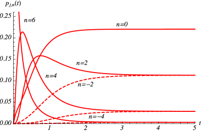
(a) $\lambda=0.6,\mu=0.6,\xi=0.5,j=6$

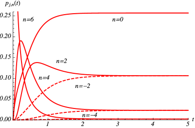
(b) $\lambda=0.6,\mu=0.6,\xi=1.0,j=6$

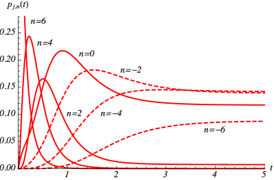
(c) $\lambda=0.2,\mu=0.6,\xi=0.5,j=6$

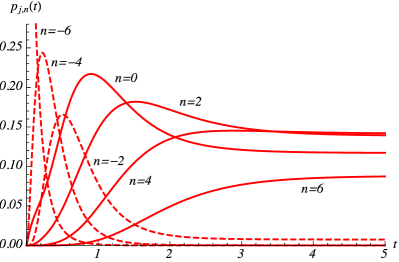
(d) $\lambda=0.6,\mu=0.2,\xi=0.5,j=-6$

Figure 3: Transient probabilites $p_{j,n}(t)$ for $N=10$.

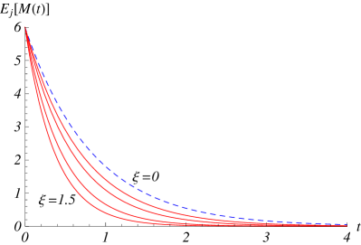
(a) $\lambda=0.6,\mu=0.6$

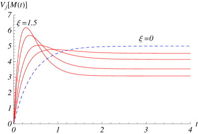
(b) $\lambda=0.6,\mu=0.6$

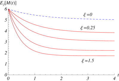
(c) $\lambda=0.6,\mu=0.2$

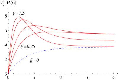
(d) $\lambda=0.6,\mu=0.2$

Figure 4: The mean and the variance of $M(t)$ for $j=6$, $N=10$ and $\xi=0.25,0.5,1.0,1.5$. The dashed curves indicate the mean and the variance of $\widetilde{M}(t)$.

In analogy with (13), from (LABEL:eq:pjnt) one can obtain the following symmetry property, with obvious notation:

$$p_{j,n}(t;\lambda,\mu)=p_{-j,-n}(t;\mu,\lambda),\qquad j,n\in S,\;\;t\geq 0.$$ (20)

Some plots of the transient probabilities (LABEL:eq:pjnt) are given in Figure 3. From cases (a) and (b) we see that $p_{j,0}(t)$ increases when $\xi$ grows. Cases (c) and (d) show instances where the symmetry property (20) is satisfied.

From relation (7), the moments of $M(t)$ can be evaluated making use of the moments of the process $\widetilde{M}(t)$. Specifically, recalling (14) and (15), for $t\geq 0$ one has:

$$E_{j}[M(t)]\!\! = \!\!je^{-(\lambda+\mu+\xi)t}+\frac{(\lambda-\mu)N}{\lambda+\mu+\xi}\left(1-e^{-(\lambda+\mu+\xi)t}\right),$$ (21)

$$E_{j}[M^{2}(t)]\!\! = \!\!\frac{N}{(\lambda+\mu+\xi)[\xi+2(\lambda+\mu)]}\Big{\{}4\lambda\mu+2N(\mu-\lambda)^{2}+\xi(\lambda+\mu)\Big{\}}$$ (22)

$$+ \!\!\frac{(\mu-\lambda)(1-2N)}{(\lambda+\mu)(\lambda+\mu+\xi)}[N(\mu-\lambda)+j(\lambda+\mu+\xi)]e^{-(\lambda+\mu+\xi)t}$$

$$+ \!\!\frac{1}{(\lambda+\mu)[\xi+2(\lambda+\mu)]}\Big{\{}2N^{2}(\mu-\lambda)^{2}-2N(\lambda^{2}+\mu^{2})-j\xi(\mu-\lambda)-2j(\mu^{2}-\lambda^{2})$$

$$+ \!\!4jN(\mu^{2}-\lambda^{2})+2j\xi N(\mu-\lambda)+2j^{2}(\lambda+\mu)^{2}+j^{2}\xi(\lambda+\mu)\Big{\}}e^{-(2\lambda+2\mu+\xi)t}.$$

Hence, in the limit we obtain

$$\lim_{t\to+\infty}E_{j}[M(t)]\!\! = \!\!\frac{(\lambda-\mu)N}{\lambda+\mu+\xi},$$

$$\lim_{t\to+\infty}E_{j}[M^{2}(t)]\!\! = \!\!N\,\frac{4\lambda\mu+2N(\mu-\lambda)^{2}+\xi(\lambda+\mu)}{(\lambda+\mu+\xi)[\xi+2(\lambda+\mu)]}\,.$$

In Figure 4 we provide some plots of mean and variance of $M(t)$ and $\widetilde{M}(t)$. We point out that $E_{j}[M(t)]$ is increasing in $t\geq 0$ if $j<\frac{(\lambda-\mu)N}{\lambda+\mu+\xi}$, whereas it is decreasing in $t\geq 0$ if the inequality is reversed.

We conclude this section by noting that, if $\lambda=\mu$, by virtue of (8) and (17) the first-passage-time density of $\widetilde{M}(t)$ through state 0, with $\widetilde{M}(0)=j$, can be expressed as follows:

$$g_{j,0}(t)=e^{-\xi t}\mu(N+1)\,{\rm sgn}(j)[\widetilde{p}_{j,1}(t)-\widetilde{p}_{j,-1}(t)]+\xi\,e^{-\xi t}\left[1-\mu(N+1)\,{\rm sgn}(j)\int_{0}^{t}[\widetilde{p}_{j,1}(\tau)-\widetilde{p}_{j,-1}(\tau)]\,d\tau\right],$$

for $j\in S\setminus\{0\}$, $t\geq 0$. Some plots are shown in Figure 5. Note that, due to (8), we have $g_{j,0}(0)=\xi$.

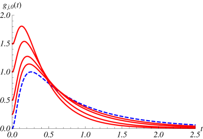
(a) $\lambda=0.6,\mu=0.6,j=3$

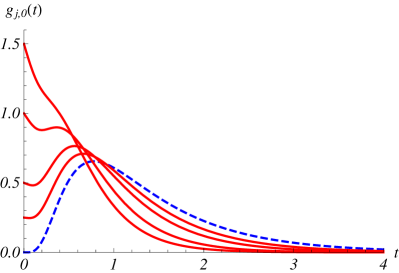
(b) $\lambda=0.6,\mu=0.6,j=6$

Figure 5: The first passage time density $g_{j,0}(t)$ for $N=10$ and $\xi=0.25,0.5,1.0,1.5$ (bottom up near the origin). The dashed curves indicate $\widetilde{g}_{j,0}(t)$.

3 A jump-diffusion approximation

We point out that the expressions obtained in Eqs. (18) and (LABEL:eq:pjnt) are computationally intractable when $N$ is large. This is compelling us to adopt an approximation procedure aiming to obtain quantitative results that are effective for large times. We recall that Kac [25] employed a typical scaling procedure in order to obtain a diffusion approximation of the discrete-time Ehrenfest model leading to the Ornstein-Uhlenbeck process (see, also, Hauert et al. [23]). By adopting a similar scaling, in this section we propose a jump-diffusion approximation for the process $M(t)$. We first rename the parameters related to the birth and death rates, given in Eqs. (1) and (2), by setting

$$\lambda=\frac{\alpha}{2}+\frac{\gamma}{2}\,\epsilon,\qquad\mu=\frac{\alpha}{2}-\frac{\gamma}{2}\,\epsilon,$$ (23)

with $\epsilon>0$, $\alpha>0$ and $-\frac{\alpha}{\epsilon}<\gamma<\frac{\alpha}{\epsilon}$. Note that $\epsilon$ is a positive constant that plays a relevant role in the approximating procedure.

For all $t\geq 0$, consider the position $M^{*}_{\epsilon}(t)=M(t)\,\epsilon$, so that $\{M^{*}_{\epsilon}(t),\;t\geq 0\}$ is a continuous-time stochastic process with state-space $\{-N\epsilon,-N\epsilon+\epsilon,\ldots,-\epsilon,0,\epsilon,\ldots,N\epsilon-\epsilon,N\epsilon\}$ and transient probabilities, for $j,n\in S$ and $t\geq 0$,

$$p^{*}_{j,n}(t)\!\! := \!\!P\left\{M^{*}_{\epsilon}(t)=n\epsilon\,|\,M^{*}_{\epsilon}(0)=j\epsilon\right\}$$ (24)

$$= \!\!P\left\{n\epsilon\leq M^{*}_{\epsilon}(t)<(n+1)\epsilon\,|\,M^{*}_{\epsilon}(0)=j\epsilon\right\}\equiv p_{j,n}(t).$$

Under suitable limit conditions the scaled process $M^{*}_{\epsilon}(t)$ converges weakly to a jump-diffusion process $\{X(t);\;t\geq 0\}$ having state-space $\mathbb{R}$ and transition density

$$f(x,t\,|\,y)=\frac{\partial}{\partial x}P\left\{X(t)\leq x\,|\,X(0)=y\right\},\qquad t\geq 0.$$

Indeed, with reference to system (4), we make use of (24) and assume that $p^{*}_{j,n}(t)\simeq f(x,t\,|\,y)\,\epsilon$ for $\epsilon$ close to 0, with $x=n\epsilon$ and $y=j\epsilon$, and expand $f$ as Taylor series, with

$$\epsilon\to 0^{+},\qquad N\to+\infty,\qquad N\epsilon\to+\infty,\qquad N\epsilon^{2}\to\nu>0.$$ (25)

We point out that, due to limits (25), the positions (23) imply that the birth and death parameters $\lambda$ and $\mu$ both tend to $\alpha/2$. We also remark that the above scaling procedure does not affect the catastrophe rate (3).

Hence, under limits (25), from the first and second equation of (4) we obtain the following partial differential equation, with $x\in\mathbb{R}$, $y\in\mathbb{R}$, $t\geq 0$:

$${\partial\over\partial t}\,f(x,t\,|\,y)={\partial\over\partial x}\left\{(\alpha x-\gamma\nu)f(x,t\,|\,y)\right\}+{1\over 2}\,{\partial^{2}\over\partial x^{2}}\left\{\alpha\nu f(x,t\,|\,y)\right\}-\xi\,f(x,t\,|\,y)+\xi\,\delta(x),$$ (26)

whereas from the third and fourth equation of (4) we have

$$\lim_{x\to\pm\infty}f(x,t\,|\,y)=0,$$

for $t\geq 0$ and $y\in\mathbb{R}$. Moreover, initial condition (5) gives the following delta-Dirac initial condition:

$$\lim_{t\to 0^{+}}f(x,t\,|\,y)=\delta(x-y).$$ (27)

We remark that Eq. $(\ref{eq:equdiff})$ is the Fokker-Planck equation for a temporally homogeneous jump-diffusion process $\{X(t),\;t\geq 0\}$ with state-space $\mathbb{R}$, having linear drift and constant infinitesimal variance. The jumps occur with constant rate $\xi$, and each jump makes $X(t)$ instantly attain the state 0. Note that modified Fokker-Planck equations similar to $(\ref{eq:equdiff})$ have also been employed in Evans and Majumdar [16], [17] for the analysis of Brownian motion with resetting.

In the sequel, for simplicity we set

$$\beta=\frac{\gamma\nu}{\alpha}.$$ (28)

3.1 The continuous process in absence of catastrophes

We point out that if $\xi\to 0^{+}$ then (26) yields the Fokker-Planck equation of an Ornstein-Uhlenbeck process on $\mathbb{R}$, denoted by $\{\widetilde{X}(t),t\geq 0\}$, with initial condition (27), and having drift and infinitesimal variance

$$A_{1}(x)=-\alpha(x-\beta),\qquad A_{2}(x)=\alpha\nu,$$ (29)

with $\alpha>0$, $\beta\in\mathbb{R}$ and $\nu>0$. This process has state-space $\mathbb{R}$ and transition density denoted as

$$\widetilde{f}(x,t\,|\,y)=\frac{\partial}{\partial x}P\left\{\widetilde{X}(t)\leq x\,|\,\widetilde{X}(0)=y\right\},\qquad t\geq 0.$$

We remark that, due to (23) and (28), the special case $\beta=0$ arises when the birth and death rates $\lambda$ and $\mu$ are equal. In this case the drift of the approximating process becomes $A_{1}(x)=-\alpha x$ so that $\widetilde{X}(t)$ has an equilibrium point in the state $0$.

Since the dynamics of $X(t)$ and $\widetilde{X}(t)$ are closely related, here we recall some useful results concerning process $\widetilde{X}(t)$. Clearly, the transition density of $\widetilde{X}(t)$ is normal with mean and variance given respectively by

$$E_{y}[\widetilde{X}(t)]=\beta\bigl{(}1-e^{-\alpha t}\bigr{)}+y\,e^{-\alpha t},\qquad V_{y}[\widetilde{X}(t)]={\nu\over 2}\,\bigl{(}1-e^{-2\alpha t}\bigr{)}.$$ (30)

Hence, the steady-state density of $\widetilde{X}(t)$ is given by

$$\widetilde{W}(x)=\lim_{t\to+\infty}\widetilde{f}(x,t\,|\,y)=\frac{1}{\sqrt{\pi\nu}}\,\exp\left\{-\frac{(x-\beta)^{2}}{\nu}\right\},\qquad x\in\mathbb{R}.$$ (31)

Note that, from (16) and (31), for $x=n\epsilon$, making use of (23), (25) and (28), we obtain

$$\lim_{\epsilon\to 0^{+}}\frac{1}{\epsilon}\,\widetilde{q}_{n}^{(\epsilon)}=\widetilde{W}(x),\qquad x\in\mathbb{R},$$ (32)

where $\widetilde{q}_{n}^{(\epsilon)}=\lim_{t\to\infty}\widetilde{p}_{j,n}(t)$ under positions $\lambda=\frac{\alpha}{2}+\frac{\gamma}{2}\,\epsilon$ and $\mu=\frac{\alpha}{2}-\frac{\gamma}{2}\,\epsilon$.

Denoting by $\widetilde{f}_{s}(x\,|\,y)=\int_{0}^{+\infty}e^{-st}\widetilde{f}(x,t\,|\,y)\,dt$ the Laplace transform of $\widetilde{f}(x,t\,|\,y)$ one has (see [37])

$$\widetilde{f}_{s}(x\,|\,y)\!\! = \!\!{2^{s/\alpha-1}\over\pi\alpha\sqrt{\nu}}\,\Gamma\biggl{(}{s\over 2\alpha}\biggr{)}\,\Gamma\biggl{(}{1\over 2}+{s\over 2\alpha}\biggr{)}\,\exp\biggl{\{}-{(x-y)(x+y-2\beta)\over 2\nu}\biggr{\}}$$ (33)

$$\times \!\!{\displaystyle D_{-s/\alpha}\biggl{(}-{\sqrt{2\over\nu}}\,((x\wedge y)-\beta)\biggr{)}\,D_{-s/\alpha}\biggl{(}{\sqrt{2\over\nu}}\,((x\vee y)-\beta)}\biggr{)},\qquad s>0,$$

where, as usual, $\wedge$ and $\vee$ mean $\min$ and $\max$, respectively, and $\Gamma(\nu)$ denotes the Euler gamma function. Moreover, $D_{-\nu}(x)$ is the parabolic cylinder function defined as (cf. [22], p. 1028, no. 9.240)

$$D_{p}(z)=2^{p/2}e^{-z^{2}/4}\Biggl{\{}{\displaystyle{\sqrt{\pi}\over\Gamma\bigl{(}{1-p\over 2}\bigr{)}}}\,\phi\Bigl{(}-{p\over 2},{1\over 2};{z^{2}\over 2}\Bigr{)}-{\displaystyle{\sqrt{2\pi}\,z\over\Gamma\bigl{(}-\,{p\over 2}\bigr{)}}}\,\phi\Bigl{(}{1-p\over 2},{3\over 2};{z^{2}\over 2}\Bigr{)}\Biggr{\}}$$

in terms of the Kummer function

$$\phi(a,c;x)=1+\sum_{n=1}^{\infty}{(a)_{n}\over(c)_{n}}\,{x^{n}\over n!}.$$

Let us denote by

$$\widetilde{T}_{y}=\inf\{t\geq 0:\widetilde{X}(t)=0\},\qquad y\in\mathbb{R}\setminus\{0\},$$ (34)

the first-passage time of $\widetilde{X}(t)$ through 0, with $\widetilde{X}(0)=y$, and let $\widetilde{g}(0,t\,|\,y)$ be the corresponding density. For $y\in\mathbb{R}\setminus\{0\}$, the Laplace transform of the first-passage time density of $\widetilde{X}(t)$ from $y$ to 0 is given by (cf. [37]):

$$\widetilde{g}_{s}(0\,|\,y)=\exp\biggl{\{}{y\over 2\nu}\bigl{(}y-2\beta\bigr{)}\biggr{\}}\;{\displaystyle{D_{-s/\alpha}\biggl{(}{\rm sgn}(y)(y-\beta)\,{\sqrt{2\over\nu}}\biggr{)}}\over{\displaystyle D_{-s/\alpha}\biggl{(}-{\rm sgn}(y)\beta\,{\sqrt{2\over\nu}}\,\biggr{)}}},\qquad s>0,$$ (35)

where ${\rm sgn}(j)=1$ if $j>0$, ${\rm sgn}(j)=-1$ if $j<0$ and ${\rm sgn}(0)=0$. Moreover, if $\beta=0$, since

$$D_{\nu}(0)=\sqrt{\pi}\,2^{\nu/2}\Bigl{[}\Gamma\Bigl{(}{1-\nu\over 2}\Bigr{)}\Bigr{]}^{-1},$$ (36)

from (35) it follows

$$\widetilde{g}_{s}(0\,|\,y)={2^{s/(2\alpha)}\over\sqrt{\pi}}\,\Gamma\Bigl{(}{1\over 2}+{s\over 2\alpha}\Bigr{)}\,\exp\biggl{\{}{y^{2}\over 2\nu}\biggr{\}}\;D_{-s/a}\biggl{(}\sqrt{2\over\nu}|y|\biggr{)},\qquad y\neq 0.$$ (37)

Finally, when $\beta=0$, taking the inverse Laplace transform of (37), for $t\geq 0$ one has the first-passage-time density

$$\widetilde{g}(0,t\,|\,y)={2\alpha|y|e^{-\alpha t}\over\sqrt{\pi\nu}\left(1-e^{-2\alpha t}\right)^{3/2}}\exp\biggl{\{}-\,{y^{2}e^{-2\alpha t}\over\nu(1-e^{-2\alpha t})}\biggr{\}},\qquad y\neq 0.$$ (38)

3.2 Analysis of the jump-diffusion process

The stochastic process $X(t)$ approximating $M(t)$ is an Ornstein-Uhlenbeck jump-diffusion process with jumps that occur with rate $\xi$. We remark that certain features of this process have been considered in the paper by Pal [34]. The main characteristics of $X(t)$ can be expressed in terms of the analogue functions of the process $\widetilde{X}(t)$ in the absence of catastrophes. Indeed, similarly as Eq. (6) the transition density of $X(t)$ satisfies the following relation:

$$f(x,t\,|\,y)=e^{-\xi t}\widetilde{f}(x,t\,|\,y)+\xi\int_{0}^{t}e^{-\xi\tau}\widetilde{f}(x,\tau\,|\,0)d\tau,\qquad x,y\in\mathbb{R},\;\;t\geq 0.$$ (39)

This equation has been succesfully exploited in various investigations in the past (cf., for instance [9] and [20]).

One immediately determines the steady-state density of $X(t)$. Indeed, from (39), it follows:

$$W(x)=\lim_{t\to+\infty}f(x,t\,|\,y)=\xi\,\widetilde{f}_{\xi}(x\,|\,0),$$ (40)

where $\widetilde{f}_{\xi}(x\,|\,y)$ is the Laplace transform of the transition density of $\widetilde{X}(t)$. Hence recalling (33) we have

$$W(x)={2^{\xi/\alpha}\over\pi\sqrt{\nu}}\,\Gamma\biggl{(}1+{\xi\over 2\alpha}\biggr{)}\,\Gamma\biggl{(}{1\over 2}+{\xi\over 2\alpha}\biggr{)}\,\exp\biggl{\{}-{x\,(x-2\beta)\over 2\,\nu}\biggr{\}}$$

$$\hskip 36.98866pt\times D_{-\xi/\alpha}\biggl{(}{\rm sgn}(x)\,\beta\sqrt{2\over\nu}\biggr{)}\,D_{-\xi/\alpha}\biggl{(}{\rm sgn}(x)\,(x-\beta)\,\sqrt{2\over\nu}\biggr{)},\qquad x\in\mathbb{R}.$$ (41)

We note that the following symmetry property holds: $W(x;\beta)=W(-x;-\beta)$, for all $x\in\mathbb{R}$ and $\beta\in\mathbb{R}$. Since $D_{0}(x)=e^{-x^{2}/4}$, from (41) it immediately follows $\lim_{\xi\to 0^{+}}W(x)=\widetilde{W}(x)$, with $\widetilde{W}(x)$ given in (31).

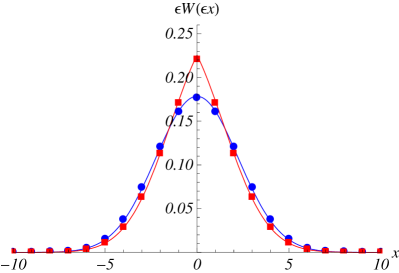
(a) $\lambda=0.6,\mu=0.6,\xi=0.5,$

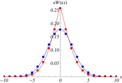
(b) $\lambda=0.6,\mu=0.6,\xi=1.0$

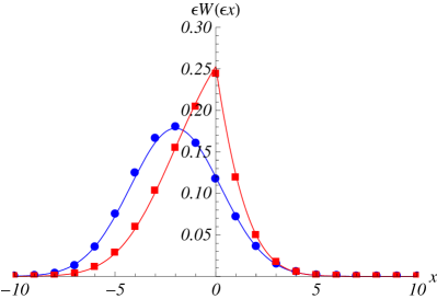
(c) $\lambda=0.2,\mu=0.3,\xi=0.5$

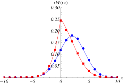
(d) $\lambda=0.3,\mu=0.2,\xi=0.5$

Figure 6: The steady-state probabilities $q_{n}$ (square) are compared with $\epsilon\,W(\epsilon\,x)$ (red curve), and $\widetilde{q}_{n}$ (circle) with $\epsilon\,\widetilde{W}(\epsilon\,x)$ (blue curve) for $N=10$ and $\epsilon=0.01$.

In order to show the goodness of the jump-diffusion approximation, recalling (32), in Figure 6 we compare the probabilities $q_{n}$ and $\widetilde{q}_{n}$ with $\epsilon\,W(\epsilon\,x)$ and $\epsilon\,\widetilde{W}(\epsilon\,x)$, respectively, for some choices of the parameters $\lambda$, $\mu$ and $\xi$. According to (23), (25) and (28), the parameters are $\nu=N\,\epsilon^{2}$, $\alpha=\lambda+\mu$, $\gamma=(\lambda-\mu)/\epsilon$ and $\beta=\gamma\nu/\alpha$. From the plots given in Figure 6 we have that (i) when $\xi$ grows the probability distributions became more peaked near $x=0$, (ii) the goodness of the approximation improves when $\lambda$ and $\mu$ are close, (iii) a symmetry arises when $\lambda$ and $\mu$ are interchanged, i.e. when $\beta$ is changed with $-\beta$.

Similarly as (7), from (39) we obtain the following relations for the moments of $X(t)$, for $k=1,2,\ldots$:

$$E_{y}[X^{k}(t)]=e^{-\xi t}E_{y}[\widetilde{X}^{k}(t)]+\xi\int_{0}^{t}e^{-\xi\tau}E_{0}[\widetilde{X}^{k}(\tau)]d\tau,\qquad y\in\mathbb{R},\;\;t\geq 0.$$ (42)

Specifically, making use of Eqs. (42) and (30) we have the conditional mean of $X(t)$:

$$E_{y}[X(t)]=ye^{-(\alpha+\xi)\,t}+{\alpha\,\beta\over\xi+\alpha}\,\bigl{[}1-e^{-(\alpha+\xi)\,t}\bigr{]},\qquad t\geq 0.$$ (43)

and the second order conditional moment:

$$E_{y}[X^{2}(t)]\!\! = \!\!{\alpha\nu\over\xi+2\alpha}+{2\alpha^{2}\beta^{2}\over(\xi+\alpha)(\xi+2\alpha)}+2\beta\Bigl{(}y-{\alpha\beta\over\xi+\alpha}\Bigr{)}\,e^{-(\xi+\alpha)\,t}$$ (44)

$$+ \!\!\Bigl{(}y^{2}-2\beta y+{2\alpha\beta^{2}\over\xi+2\alpha}-{\alpha\nu\over\xi+2\alpha}\Bigr{)}e^{-(\xi+2\alpha)\,t},\qquad t\geq 0.$$

We stress that the validity of the approximating procedure given in Section 3 is confirmed by the following limits, that can be easily obtained from Eqs. (21) and (22), for $y=j\epsilon$ and making use of (23), (25) and (28):

$$\lim_{\epsilon\to 0^{+}}\epsilon\,E_{j}[{M}(t)]=E_{y}[{X}(t)],\qquad\lim_{\epsilon\to 0^{+}}\epsilon^{2}\,V_{j}[{M}(t)]=V_{y}[{X}(t)].$$

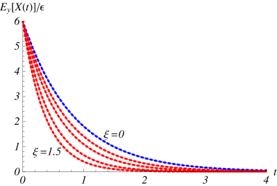
(a) $\lambda=0.6,\mu=0.6$

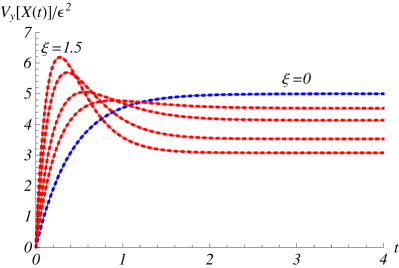
(b) $\lambda=0.6,\mu=0.6$

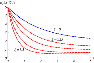
(c) $\lambda=0.3,\mu=0.2$

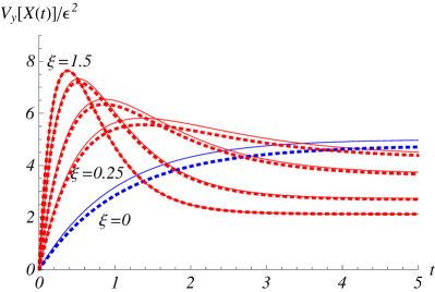
(d) $\lambda=0.3,\mu=0.2$

Figure 7: The mean and the variance of $M(t)$ for $j=6$, $N=10$ and $\xi=0,0.25,0.5,1.0,1.5$ (dotted curves) are compared with $E_{y}[X(t)]/\epsilon$ and $V_{y}[X(t)]/\epsilon^{2}$ (solid curves) with $\epsilon=0.01$ and $y=j\epsilon$.

In Figure 7 we compare the mean $E_{j}[M(t)]$ and the variance $V_{j}[M(t)]$ with $E_{y}[X(t)]/\epsilon$ and $V_{y}[X(t)]/\epsilon^{2}$, respectively, for various choices of the parameters $\lambda$, $\mu$ and $\xi$. According to (23), (25) and (28), the parameters are $\nu=N\,\epsilon^{2}$, $\alpha=\lambda+\mu$, $\gamma=(\lambda-\mu)/\epsilon$, $\beta=\gamma\nu/\alpha$ and $y=j\epsilon$, so that from (21) and (43) one has $E_{j}[M(t)]=E_{y}[X(t)]/\epsilon$. Furthermore, from the plots (b) and (d) of Figure 7 we note that the goodness of the approximation for the variances improves when $\lambda$ and $\mu$ are close.

Similarly as (34), let us denote by $T_{y}$ the first-passage time of $X(t)$ through 0, with $X(0)=y$, and let $g(0,t\,|\,y)$ be the corresponding density. The densities $\widetilde{g}(0,t\,|\,y)$ and $g(0,t\,|\,y)$, for $t\geq 0$ are related as follows (see, for instance, [20]):

$$g(0,t\,|\,y)=e^{-\xi\,t}\widetilde{g}(0,t\,|\,y)+\xi\,e^{-\xi\,t}\biggl{[}1-\int_{0}^{t}\widetilde{g}(0,\tau\,|\,y)d\tau\biggr{]},\qquad y\neq 0.$$ (45)

Considering the Laplace transforms in (45) one has

$$g_{s}(0\,|\,y)={s\over s+\xi}\,\tilde{g}_{s+\xi}(0\,|\,y)+{\xi\over s+\xi},\qquad s>0,$$ (46)

with $\tilde{g}_{s+\xi}(0\,|\,y)$ given in (35). From (46) it follows that $P(T_{y}<+\infty)=1$, so that the first passage through 0 occurs almost surely. The moments of $T_{y}$ can thus be evaluated by means of (46) making use of (35). In particular, for $y\neq 0$ we have:

$$E[T_{y}]={1\over\xi}\,\bigl{[}1-\tilde{g}_{\xi}(0|y)\bigr{]}={1\over\xi}\,\left[1-\exp\biggl{\{}{y\over 2\nu}\bigl{(}y-2\beta\bigr{)}\biggr{\}}\;{\displaystyle{D_{-\xi/\alpha}\biggl{(}{\rm sgn}(y)(y-\beta)\,{\sqrt{2\over\nu}}\biggr{)}}\over{\displaystyle D_{-\xi/\alpha}\biggl{(}-{\rm sgn}(y)\beta\,{\sqrt{2\over\nu}}\,\biggr{)}}}\right],$$ (47)

and the second order moment can be obtained from

$$E[T_{y}^{2}]={2\over\xi^{2}}\,\Bigl{[}1-\tilde{g}_{\xi}(0|x_{0})+\xi\,{d\over d\xi}\,\tilde{g}_{\xi}(0|x_{0})\Bigr{]}.$$

3.3 A special case

We now assume that $\beta=0$. Recalling Eqs. (23) and (28), this assumption corresponds to the condition $\lambda=\mu$. In other terms, in this case the process $M(t)$ is symmetric (see Eq. (20)), and also the jump-diffusion process $X(t)$ reflects such a symmetry. From (39), one has (cf. [20]):

$$f(x,t|y)=e^{-\xi t}\widetilde{f}(x,t|y)+{2^{\xi/(2\alpha)}\over\sqrt{\pi\nu}}\Gamma\Bigl{(}1+{\xi\over 2\alpha}\Bigr{)}\exp\Bigl{\{}-{x^{2}\over 2\nu}\Bigr{\}}D_{-\xi/\alpha}\Bigl{(}|x|\sqrt{2\over\nu}\Bigr{)}$$

$$\hskip 14.22636pt-{\xi\over 2\alpha\sqrt{\pi\nu}}\sum_{k=0}^{+\infty}(-1)^{k}{{\xi\over 2\alpha}-1\choose k}\Biggl{[}\exp\Bigl{\{}-{x^{2}\over\nu}\Bigr{\}}\Psi\Bigl{(}1,{1\over 2}-k;{x^{2}\over\nu}\Bigl{)}$$

$$\hskip 14.22636pt-\bigl{(}1-e^{-2\alpha t}\bigr{)}^{k+1/2}\exp\Bigl{\{}-{x^{2}\over\nu\bigr{(}1-e^{-2\alpha t}\bigr{)}}\Bigr{\}}\Psi\Bigl{(}1,{1\over 2}-k;{x^{2}\over\nu\bigr{(}1-e^{-2\alpha t}\bigr{)}}\Bigl{)}\Biggr{]},$$ (48)

where $\Psi(a,b;x)$ denotes the Kummer’s function of the second kind, defined as (cf. [22], p. 1023, n. 9.210.2):

$$\Psi(a,b;x)={\Gamma(1-b)\over\Gamma(a-b+1)}\;\Phi(a,b;x)+{\Gamma(b-1)\over\Gamma(a)}\;x^{1-b}\;\Phi(a-b+1,2-b;x).$$

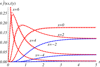
(a) $\lambda=0.6,\mu=0.6,\xi=0$

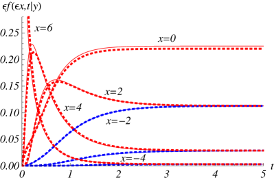
(b) $\lambda=0.6,\mu=0.6,\xi=0.5$

Figure 8: The transition probabilities $\widetilde{p}_{j,n}(t)$ and $p_{j,n}(t)$ (dotted curves) for $j=6$ and $N=10$ are compared with $\epsilon\widetilde{f}(\epsilon x,t|y)$ and $\epsilon f(\epsilon x,t|y)$ (solid curves), respectively, with $\epsilon=0.01$ and $y=j\epsilon$.

For $\lambda=\mu=0.6$, in Figure 8 we compare the transition probability $\widetilde{p}_{j,n}(t)$ with $\epsilon\widetilde{f}(\epsilon x,t|y)$ for $\xi=0$ in (a) and the transition probability $p_{j,n}(t)$ with $\epsilon f(\epsilon x,t|y)$ for $\xi=0.5$ in (b). According to (23), (25) and (28), the parameters are $\nu=N\,\epsilon^{2}$, $\alpha=2\mu$, $\gamma=\beta=0$ and $y=j\epsilon$.

Finally, in the special case $\beta=0$, making use of (38) in (45), for the process $X(t)$ we obtain

$$g(0,t\,|\,y)=e^{-\xi t}\,\widetilde{g}(0,t\,|\,y)+\xi\,e^{-\xi t}{\rm Erf}\biggl{(}|y|e^{-\alpha t}\,\sqrt{1\over\nu(1-e^{-2\alpha t})}\biggr{)},\qquad t\geq 0\quad y\neq 0,$$ (49)

where ${\rm Erf}(\cdot)$ is the error function, and $\widetilde{g}(0,t\,|\,y)$ is given in (38).

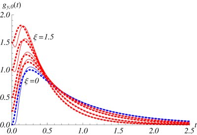
(a) $\lambda=0.6,\mu=0.6,j=3$

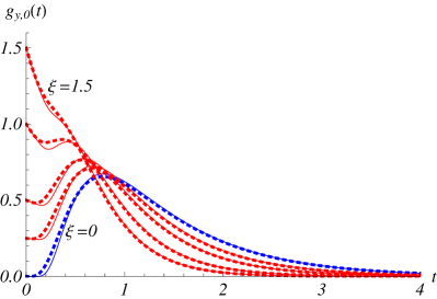
(b) $\lambda=0.6,\mu=0.6,j=6$

Figure 9: The first passage time density $g_{j,0}(t)$ (dotted curves) for $N=10$ and $\xi=0,0.25,0.5,1.0,1.5$ (bottom up near the origin) are compared with $g(0,t|y)$ (solid curves) with $\epsilon=0.01$ and $y=j\epsilon$.

In Figure 9 we compare the first passage time density $g_{j,0}(t)$ with $g(0,t|y)$ for $\lambda=\mu$ and various choices of $\xi$. According to (23), (25) and (28), the parameters are $\nu=N\,\epsilon^{2}$, $\alpha=2\mu$, $\gamma=\beta=0$ and $y=j\epsilon$. We note that the goodness of the approximation improves when $t$ increases.

Moreover, due to (37) and (47), and recalling (36), for $\beta=0$ one has the mean first passage time:

$$E[T_{y}]={1\over\xi}\,\left[1-{2^{\xi/(2\alpha)}\over\sqrt{\pi}}\,\Gamma\Bigl{(}{1\over 2}+{\xi\over 2\alpha}\Bigr{)}\,\exp\biggl{\{}{y^{2}\over 2\nu}\biggr{\}}\;D_{-\xi/a}\biggl{(}\sqrt{2\over\nu}|y|\biggr{)}\right],\qquad y\neq 0.$$ (50)

The goodness of the continuous approximation is also confirmed by the results obtained for the first passage times. Indeed, Figure 10 shows some plots of the mean and variance of the first-passage-time of ${\cal T}_{y}$ and $T_{y}$, for some choices of the parameters, with $0\leq\xi\leq 5$, and for parameters $\nu=N\,\epsilon^{2}$, $\alpha=2\mu$, $\gamma=\beta=0$ and $y=j\epsilon$. We remark that $E[{\cal T}_{j}]$, $V[{\cal T}_{j}]$ and $V[T_{y}]$ have been obtained by means of numerical calculations, whereas $E[T_{y}]$ is obtained from (50). It is clear that the means and variances are decreasing when $\xi$ increases. This fact confirms that the presence of the catastrophes has a regulatory effect on the considered stochastic system.

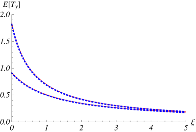
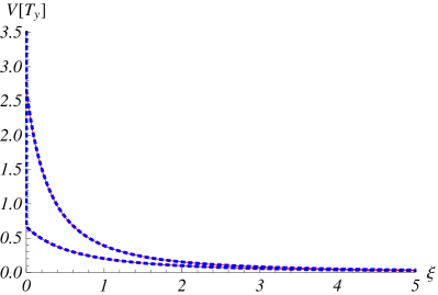
Figure 10: The mean $E[{\cal T}_{j}]$ and the variance $V[{\cal T}_{j}]$ (dotted curves) for $j=3$, $N=10$ and $\lambda=\mu=0.3,0.6$ (top to bottom) are compared with $E[T_{y}]$ and $V[T_{y}]$ (solid curves), respectively, with $\epsilon=0.01$ and $y=j\epsilon$.

References

- [1] Balaji, S.; Mahmoud, H.; Tong, Z.: Phases in the diffusion of gases via the Ehrenfest urn model. J. Appl. Probab. 47, 841–855 (2010)
- [2] Brockwell, P.J.: The extinction time of a birth, death and catastrophe process and of a related diffusion model. Adv. Appl. Prob. 17, 42–52 (1985)
- [3] Brockwell, P.J.: The extinction time of a general birth and death process with catastrophes. J. Appl. Prob. 23, 851–858 (1986)
- [4] Cairns, B., Pollett, P.K.: Extinction times for a general birth, death and catastrophe process. J. Appl. Prob. 41, 1211–1218 (2004)
- [5] Chao, X., Zheng, Y.: Transient and equilibrium analysis of an immigration birth-death process with total catastrophes. Prob. Engin. Inf. Sci. 17, 83–106 (2003)
- [6] Chen, A., Renshaw, E.: The M/M/1 queue with mass exodus and mass arrivals when empty. J. Appl. Prob. 34, 192–207 (1997)
- [7] Chen, A., Renshaw, E.: Markovian bulk-arriving queues with state-dependent control at idle time. Adv. Appl. Prob. 36, 499–524 (2004)
- [8] Chen, A., Zhang, H., Liu, K., Rennolls, K.: Birth-death processes with disasters and instantaneous resurrection. Adv. Appl. Prob. 36, 267–292 (2004)
- [9] di Cesare, R., Giorno, V., Nobile. A.G.: Diffusion processes subject to catastrophes. In: Moreno-Diaz, R. et al., Eds. EUROCAST 2009, LNCS 5717, pp. 129–136. Springer-Verlag, Berlin, Heidelberg (2009)
- [10] Di Crescenzo, A.: First-passage-time densities and avoiding probabilities for birth-and-death processes with symmetric sample paths. J. Appl. Prob. 35, 383–394 (1998)
- [11] Di Crescenzo, A., Giorno, V., Krishna Kumar, B., Nobile, A.G.: A double-ended queue with catastrophes and repairs, and a jump-diffusion approximation. Methodol. Comput. Appl. Prob. 14, 937–954 (2012)
- [12] Di Crescenzo, A., Giorno, V., Nobile, A.G., Ricciardi, L.M.: On the M/M/1 queue with catastrophes and its continuous approximation. Queueing Syst. 43, 329–347 (2003)
- [13] Di Crescenzo, A., Giorno, V., Nobile, A.G., Ricciardi, L.M.: A note on birth-death processes with catastrophes. Stat. Prob. Lett. 78, 2248–2257 (2008)
- [14] Economou, A., Fakinos, D.: A continuous-time Markov chain under the influence of a regulating point process and applications in stochastic models with catastrophes. Eur. J. Oper. Res. 149, 625–640 (2003)
- [15] Economou, A., Fakinos, D.: Alternative approaches for the transient analysis of Markov chains with catastrophes. J. Stat. Theory Pract. 2, 183–197 (2008)
- [16] Evans, M.R., Majumdar, S.N.: Diffusion with stochastic resetting. Phys. Rev. Lett. 106, 160601 (2011)
- [17] Evans, M.R., Majumdar, S.N.: Diffusion with optimal resetting. J. Phys. A Math. Theor. 44, 435001 (2011)
- [18] Flegg, M.B., Pollett, P.K., Gramotnev, D.K.: Ehrenfest model for condensation and evaporation processes in degrading aggregates with multiple bonds. Phys. Rev. E 78, 031117 (2008)
- [19] Giorno, V., Nobile, A.G.: On a bilateral linear birth and death process in the presence of catastrophes, in: R. Moreno-Daz, F.R. Pichler, A. Quesada-Arencibia (Eds.), Computer Aided Systems Theory - EUROCAST 2013, Lecture Notes in Computer Science, vol. 8111, Springer-Verlag, 2013, pp. 28–35.
- [20] Giorno, V., Nobile, A.G., di Cesare, R.: On the reflected Ornstein-Uhlenbeck process with catastrophes. Appl. Math. Comput. 218, 11570–11582 (2012)
- [21] Giorno, V., Nobile, A.G., Spina, S.: On some time non-homogeneous queueing systems with catastrophes. Appl. Math. Comput. 245, 220–234 (2014)
- [22] Gradshteyn, I.S., Ryzhik, I.M.: Tables of Integrals, Series and Products, 7th edn. Academic Press, Amsterdam (2007)
- [23] Hauert, Ch., Nagler, J., Schuster, H.G.: Of dogs and fleas: the dynamics of N uncoupled two-state systems. J. Stat. Phys. 116, 1453–1469 (2004)
- [24] Iglehart, D.L.: Limit theorems for the multi-urn Ehrenfest model. Ann. Math. Statist. 39, 864–876 (1968)
- [25] Kac, M.: Random walk and the theory of Brownian motion. Amer. Math. Monthly 54, 369–391 (1947)
- [26] Kusmierz, L., Majumdar, S.N., Sabhapandit, S., Schehr, G.: First order transition for the optimal search time of Lévy flights with resetting. Phys. Rev. Lett. 113, 220602 (2014)
- [27] Krishna Kumar, B., Krishnamoorthy, A., Pavai Madheswari, S., Sadiq Basha, S., Transient analysis of a single server queue with catastrophes, failures and repairs, Queueing Syst. 56, 133–141 (2007)
- [28] Krishna Kumar, B., Vijayakumar, A., Sophia, S.: Transient analysis for state-dependent queues with catastrophes. Stoch. Anal. Appl. 26, 1201–1217 (2008)
- [29] Kyriakidis, E.G.: Stationary probabilities for a simple immigration-birth-death process under the influence of total catastrophes. Stat. Prob. Lett. 20, 239–240 (1994)
- [30] Kyriakidis, E.G.: The transient probabilities of the simple immigration-catastrophe process. Math. Sci. 26, 56–58 (2001)
- [31] Kyriakidis, E.G.: The transient probabilities of a simple immigration-emigration-catastrophe process. Math. Sci. 27, 128–129 (2002)
- [32] Kyriakidis, E.G.: Transient solution for a simple immigration birth-death process. Prob. Eng. Inf. Sci. 18, 233–236 (2004)
- [33] Pakes, A.G.: Killing and resurrection of Markov processes. Comm. Stat. Stoch. Mod. 13, 255–269 (1997)
- [34] Pal, A.: Diffusion in a potential landscape with stochastic resetting. Phys. Rev. E 91, 012113 (2015)
- [35] Pollett, P., Zhang, H., Cairns, B.J.: A note on extinction times for the general birth, death and catastrophe process. J. Appl. Prob. 44, 566–569 (2007)
- [36] Renshaw, E., Chen, A.: Birth-death processes with mass annihilation and state-dependent immigration. Comm. Stat. Stoch. Mod. 13, 239–253 (1997)
- [37] Siegert, A.J.F.: On the first passage time probability problem. Phys. Rev. 81, 617–623 (1951)
- [38] Takahashi, H.: Ehrenfest model with large jumps in finance. Physica D 189, 61–69 (2004)
- [39] Van Doorn, E.A., Zeifman, A.: Extinction probability in a birth-death process with killing. J. Appl. Prob. 42, 185–198 (2005)
- [40] Zeifman, A., Satin, Y., Panfilova, T.: Limiting characteristics for finite birth-death-catastrophe processes. Math. Biosci. 245, 96–102 (2013)
- [41] Zheng, Q.: Note on the non-homogeneous Prendiville process. Math. Biosci. 148, 1–5 (1998)