Black-hole microstate spectroscopy: ringdown, quasinormal modes, and echoes

Abstract

Deep conceptual problems associated with classical black holes can be addressed in string theory by the “fuzzball” paradigm, which provides a microscopic description of a black hole in terms of a thermodynamically large number of regular, horizonless, geometries with much less symmetry than the corresponding black hole. Motivated by the tantalizing possibility to observe quantum gravity signatures near astrophysical compact objects in this scenario, we perform the first $3+1$ numerical simulations of a scalar field propagating on a large class of multicenter geometries with no spatial isometries arising from ${\cal N}=2$ four-dimensional supergravity. We identify the prompt response to the perturbation and the ringdown modes associated with the photon sphere, which are similar to the black-hole case, and the appearance of echoes at later time, which is a smoking gun of some structure at the horizon scale and of the regular interior of these solutions. The response is in agreement with an analytical model based on geodesic motion in these complicated geometries. Our results provide the first numerical evidence for the dynamical linear stability of fuzzballs, and pave the way for an accurate discrimination between fuzzballs and black holes using gravitational-wave spectroscopy.

I Introduction

Within Einstein’s theory of General Relativity, black holes (BHs) are the simplest macroscopic objects one can conceive. In stationary configurations, they are fully described only by their mass, spin, and possibly electric charge [1, 2, 3, 4], being in this respect more akin to elementary particles than to astrophysical objects [5]. This simplicity is also associated with a high degree of symmetry: stationary BHs must be axisymmetric [6], and become spherical in the static (i.e., non-spinning) limit.

Owing to this and other remarkable properties, the equations governing the linear response of a BH to external perturbations and its quick relaxation towards stationarity after being formed (e.g., in a merger or in a stellar collapse) are separable in terms of a simple set of ordinary differential equations [7, 8], which enormously simplifies the analysis of BH linear perturbations. The latter are crucial, for instance, to describe the so-called “ringdown” during the post-merger phase of a binary coalescence [9]. The BH ringdown is governed by a discrete set of complex frequencies – the so-called quasinormal modes (QNMs) – which are uniquely determined by the BH parameters. BH spectroscopy [10, 11, 12, 13, 14, 15, 16, 17, 18] performed by measuring the ringdown with current and future gravitational-wave detectors [19, 20, 21] is at present the most robust way to study the strong-field regime of General Relativity and the nature of a merger remnant [22, 19, 20, 23]. Indeed, BHs can be considered as the “hydrogen atom” of gravity, and their gravitational-wave spectrum is a unique footprint of possible deviations from General Relativity in the strong-field regime, similarly to the energy levels of the hydrogen whose measurement had a paramount impact in shaping the development of quantum electrodynamics [24].

This state of affairs is enormously more involved when the spacetime fails to be as simple and as symmetric as a BH. This happens arguably in any quantum gravity proposal aiming at resolving some outstanding issues with classical BHs [25], namely the curvature singularities that are conjectured to be always covered by event horizons [26, 27, 28], the conundrum of the huge BH entropy [29, 30], and the unitarity-loss problem associated with Hawking evaporation at the semiclassical level [31].

In the string-theory “fuzzball” proposal [32, 33, 34, 35], a classical BH is described by an ensemble of smooth and horizonless geometries which represent the microstates of the BH with the same mass and asymptotic charges. The classical properties of a BH are expected to emerge either through an averaging procedure over a large number of microstates or as a ‘collective behavior’ of fuzzballs. Although finding a statistically significant number of microstate geometries in order to account for the whole BH entropy is challenging, large families of microstates have been discovered in the last few years [36, 37, 38, 39, 40, 41]. A microscopic description of the whole entropy is provided by D-brane counting for BPS black holes in four and five dimensions [42, 43, 44]. Should the fuzzball program be successful, it would be a natural solution to the singularity, entropy, and unitarity problems that plague the classical BH interpretation.

Fuzzball microstates are much less symmetric than a BH. Besides being stationary solutions to consistent low-energy truncations of string theory, fuzzballs do not generically possess any spatial isometry. This lack of symmetry and the complexity of the microstate geometries have so far hampered the possibility to study their ringdown and multipole structure [45, 46, 47, 48, 49, 50, 51, 52, 53] and to compare it with the one of a BH, which is a task of utmost importance to devise phenomenological tests of the fuzzball paradigm – and hence of quantum gravity – with gravitational-wave data [54].

In order to overcome this problem, in this work we perform for the first time $3+1$ numerical simulations of small fields propagating on a large class of a microstate geometries. We unveil the entire ringdown phenomenology [55, 56] predicted in somehow less motivated models of exotic compact objects.

This includes the universal prompt ringdown similar to the BH case, which is nonetheless followed by a modulated series of repeated “echoes” [57, 58] associated with long-lived modes almost trapped within the fuzzball gravitational potential, providing a smoking gun of some extra structure at the horizon scale [59, 60, 61, 62, 63, 64, 65, 66, 67, 68, 69, 70, 56, 71]. These ringdown features are currently searched for in gravitational-wave data [72, 73, 61, 74, 75, 76, 77, 78, 23] (see [55, 79] for some reviews). Finally, we provide a simple physical interpretation of these effects in terms of the geodesics and multipolar structure of these complicated microstate geometries. We use natural units throughout.

II Fuzzball geometries

Our framework is that of ${\cal N}=2$ four-dimensional supergravity, wherein gravity is (non-)minimally coupled to four $U(1)$ gauge fields and three complex scalars. Microstates of spherically symmetric 4-dimensional BHs can be constructed in this theory by considering a multi-center system of intersecting D3-branes [80, 81, 82, 40]. The metric reads

$$ds^{2}=-e^{2U}(dt+\omega)^{2}+e^{-2U}\sum_{i=1}^{3}dx^{2}_{i},$$ (1)

with

$$e^{-4U} =Z_{1}Z_{2}Z_{3}V-\mu^{2}V^{2}\,,$$ (2)

$$*_{3}d\omega ={\textstyle\frac{1}{2}}\left(VdW-WdV+K^{I}dL_{I}-L_{I}dK^{I}\right)\,,$$

and

$$Z_{I} = L_{I}+\frac{\left|\epsilon_{IJK}\right|}{2}\frac{K^{J}K^{K}}{V}\,,$$ (3)

$$\mu = \frac{W}{2}+\frac{L_{I}K^{I}}{2V}+{\left|\epsilon_{IJK}\right|}{}\frac{K^{I}K^{J}K^{K}}{6V^{2}}$$ (4)

where $\epsilon_{IJK}$ is the totally antisymmetric tensor, and $\{V,L_{I},K^{I},W\}$ are eight harmonic functions ($I=1,2,3$). As an ansatz, we take $N$-center harmonic functions of the form

$$V = 1+\sum_{a=1}^{N}{v_{a}\over|\vec{x}-\vec{x}_{a}|}\,,\quad L_{I}=1+\sum_{a=1}^{N}{{\ell}_{I,a}\over|\vec{x}-\vec{x}_{a}|}\,,$$ (5)

$$K^{I} = \sum_{a=1}^{N}{k^{I}_{a}\over|\vec{x}-\vec{x}_{a}|}\,,\quad\hskip 17.07182ptW=\sum_{a=1}^{N}{m_{a}\over|\vec{x}-\vec{x}_{a}|}\,,$$ (6)

with $\vec{x}=r(\sin\theta\,\cos\phi,\sin\theta\,\sin\phi,\cos\theta)$ . From a four-dimensional perspective these microstate geometries are singular at the centers but, for specific choice of charges and positions of the centers, they admit a regular horizonless five-dimensional uplift. Overall, the solution is regular, horizonless, and free of other pathologies (e.g., closed timelike curves). In general it carries four electric $Q_{A}=(Q_{0},Q_{I})$ and four magnetic $P^{A}=(P^{0},P^{I})$ charges. For concreteness we shall focus on $3$-center ($N=3$) solutions and restrict ourselves to $4$-charge solutions by imposing $Q_{0}=P^{I}=0$, although the generalization is straightforward. We provide their explicit form in Appendix A.

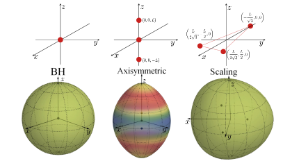
Figure 1: Top: Schematic representation of the multicenter microstate solutions considered in this work (see Appendix A for details on their construction). The leftmost BH solution corresponds to the case in which the centers coincide. The middle solution is axially and equatorially symmetric, whereas the rightmost “scaling” solution breaks the axial symmetry. Bottom: corresponding embedding diagram for each solution. The shape describes constant-$t$ and constant-$r$ surfaces of the metric deep down the fuzzball’s throat. Deformations are related to the mass multipole moments, whereas the colors are weighted according to $g_{t\phi}$ to represent the leading current multipole moments (which vanish for the BH and the scaling solution) [83, 52].

The entropy of corresponding BH is explained by the huge parameter space of the solutions, which asymptotically reduce to the 4-charge BPS BH solution [84]. The latter generalizes the extremal Reissner-Nordström BH to the case of four different charges and three scalar fields. In the isotropic coordinates, the line element of the 4-charge BH reads [84]

$$ds^{2}=-f(r)dt^{2}+f(r)^{-1}\left[dr^{2}+r^{2}(d\theta^{2}+\sin^{2}\theta d\phi^{2})\right]\,,$$ (7)

with $f(r)=\left(H_{1}H_{2}H_{3}H_{4}\right)^{-1/2}$ and $H_{A}=1+{Q_{A}\over r}$. The total mass is $M={\textstyle\frac{1}{4}}\left(Q_{1}+Q_{2}+Q_{3}+Q_{4}\right)$ (with $Q_{4}=P^{0}$ in the cases we consider). When $Q_{A}=Q$, the solution reduces to the extremal Reissner-Nordström BH with mass $M=Q$.

Although our method is general, for concreteness we shall consider some representative class of microstate geometries, depicted in Fig. 1. The first family comprises axisymmetric solutions with equatorial symmetry, i.e. reflection symmetric with respect to the equatorial plane, $\theta\to\pi-\theta$ (equivalently, $z\to-z$). They have three centers aligned along the $z$-axis, located at $\vec{x}_{a}=(0,0,z_{a})$, with

$$z_{1}=L\,,\quad z_{2}=0\,,\quad z_{3}=-L\,.$$ (8)

This is a discrete three-parameter family of solutions with nonvanishing angular momentum, whose explicit form is provided in Appendix A 2. The size L is determined in terms of the charges of the centers.

The second family of $3$-center solutions we consider are those with $v_{a}=1$, four charges, and centers located on the vertices of a triangle. This is a five-parameter family which in general breaks both axial and equatorial symmetry [83, 52]. The simplest element is the so-called “scaling” solution that corresponds to the three centers being located at the vertices of an equilateral triangle and has two free parameters – related to the mass and the size of the triangle – while the angular momentum vanishes. The explicit form of this solution is given in Appendix A.3.1.

In all cases, when the centers collapse to a single point, spherical symmetry is restored and the solution reduces to the extremal (non-rotating) BH.

III Linear response of BHs and microstates: prompt ringdown, QNMs, and echoes

We now focus on the linear dynamics of a neutral massless scalar field propagating in the metrics described in the previous section. This is governed by the Klein-Gordon equation $\square\Phi(t,r,\theta,\phi)=0.$ Decomposing $\Phi$ in spherical harmonics, i.e. $\Phi=\sum_{lm}\Phi_{lm}(r,t)Y_{lm}(\theta,\phi)$, the (orbital) angular-momentum number is an integer $l=0,1,2..$ and the azimuthal number $m$ is an integer such that $|m|\leq l$. When the metric is spherically symmetric (as in the BH case considered above), the azimuthal number is $(2l+1)$-fold degenerate and different $l$ modes are decoupled from each other. In the axisymmetric case, the degeneracy of $m$ is broken but $m$ is still a conserved quantum number: modes with different $m$ are decoupled. In the general case with no isometries, modes with different $l$ and $m$ can all mix with each others and it is more convenient to solve the Klein-Gordon equation directly as a $3+1$ evolution problem.

The prompt response of a compact object to some perturbation is universally described by the resonant excitation of its photon sphere, where (unstable) closed null orbits reside. For a BH spacetime, the photon-sphere modes coincide with the QNMs of the object and dominate the linear response [57]. The QNMs are defined in the frequency domain as those complex eigenfrequencies, $\omega=\omega_{R}+i\omega_{I}$, which correspond to a solution that satisfies purely outgoing-wave boundary conditions at infinity and “regularity” conditions at the inner boundary. In the BH case, regularity at the horizon imposes purely ingoing-wave boundary conditions, whereas in the horizonless fuzzball case $\Phi$ must be regular at the origin $r=0$. For each $(l,m)$ mode, there is a countably infinite number of QNMs identified by the overtone index $n=0,1,2,..$, with $n=0$ labelling the fundamental QNM dominating the linear response at late times.

Crucially, if the spacetime is horizonless, the photon-sphere modes dominate only the initial ringdown until the perturbation has time to probe the inner boundary. Following the universal prompt ringdown, radiation can be reflected back and get quasi-trapped within the gravitational potential of the object, occasionally tunnelling to infinity and producing a series of repeated and modulated “echoes” [57, 58, 85, 86]. This transient regime interpolates between the prompt ringdown and the very late-time behavior, which is instead dominated by the long-lived modes of the horizonless compact object [56].

III.1 Analytical results in the geodesic approximation

There exists a tight relation between the ringdown modes of a compact object and some geodesic properties associated with the existence of an unstable photon sphere, as established in the eikonal limit [87, 88]. In the static case, the real part of the QNM frequency is related to the (azimuthal) orbital frequency, whereas the imaginary part of the QNM corresponds to the Lyapunov exponent of the orbit [88]. In the rotating case the relation between modes with generic $(l,m)$ and specific geodesic quantities is more involved [89]. Strictly speaking the geodesic approximation is valid when $l\gg 1$ but it often works remarkably well also for smaller values of $l$ [90].

$\kappa$	$M$	$L/M$	$J/M^{2}$	$r_{+}/M$	$r_{-}/M$	$M\omega_{\rm QNM,+}^{\rm fuzzball}$	$M\omega_{\rm QNM,-}^{\rm fuzzball}$	$M\omega_{\rm QNM}^{\rm BH}$	$\Delta t_{+}/M$	$\Delta t_{-}/M$
3	13.75	0.1091	0.0714	0.7314	0.6759	$0.6827-0.0767i$	$0.7324-0.0878i$	$0.6996-0.0871i$	40.7	40.1
4	24.25	0.0508	0.0544	0.7596	0.6490	$0.6860-0.0841i$	$0.7372-0.0855i$	$0.7083-0.0859i$	63.8	62.7
5	37.75	0.0301	0.0439	0.7493	0.6379	$0.6919-0.0852i$	$0.7380-0.0839i$	$0.7128-0.0851i$	84.9	83.7
6	54.25	0.0201	0.0367	0.7378	0.6345	$0.6966-0.0854i$	$0.7373-0.0831i$	$0.7154-0.0847i$	105.1	104.1
7	73.75	0.0144	0.0315	0.7283	0.6343	$0.7001-0.0853i$	$0.7362-0.0827i$	$0.7170-0.0844i$	125.0	124.0
8	96.25	0.0109	0.0276	0.7207	0.6352	$0.7028-0.0852i$	$0.7351-0.0825i$	$0.7180-0.0841i$	144.6	143.7
9	121.75	0.0085	0.0246	0.7146	0.6367	$0.7050-0.0851i$	$0.7341-0.0825i$	$0.7188-0.0840i$	164.0	163.2
10	150.25	0.0069	0.0221	0.7097	0.6383	$0.7067-0.0849i$	$0.7332-0.0824i$	$0.7193-0.0839i$	183.3	182.6
50	3750	0.0003	0.0044	0.6746	0.6593	$0.7188-0.0837i$	$0.7244-0.0830i$	$0.7216-0.0834i$	942.2	942.1
100	15000	0.0001	0.0022	0.6706	0.6629	$0.7103-0.0835i$	$0.7231-0.0832i$	$0.7217-0.0833i$	1887.3	1887.2

Table 1: Summary of the ringdown features of an axisymmetric fuzzball geometry (with $\kappa_{1}=\kappa_{2}=\kappa_{3}=\kappa$) in the geodesic approximation for $l=m=\pm 2$. $M$ is the total mass, the ratio $L/M$ characterizes the distance of the centers, $J/M^{2}$ is the dimensionless angular momentum. The $\pm$ signs refers to co-rotating and counter-rotating orbits. $r_{\pm}/M$ are the dimensionless critical radii. $\Delta t_{\pm}$ is the echo time scale estimated using the WKB approximation [Eq. (20)] for co-rotating and counter-rotating orbits. For the BH case, the QNMs are in agreement with an exact frequency-domain computation (see Appendix B.2) within a few percent.

Geodesic motion for a massless neutral particle moving in the spacetime given in Eq. (1) can be described by the null Hamiltonian $\mathcal{H}=\frac{1}{2}g^{\mu\nu}P_{\mu}P_{\nu}=0$, where $P_{\mu}$ is the particle four-momentum. For simplicity we focus on the axisymmetric case, i.e. consider a stationary metric as in Eq. (1), where $\omega=\omega_{\phi}d\phi$. The Hamiltonian in this case can be written as

$$2\mathcal{H}=-e^{-2U}E^{2}+e^{2U}\left(P_{r}^{2}+\frac{P_{\theta}^{2}}{r^{2}}+\frac{\left(P_{\phi}+\omega_{\phi}E\right)^{2}}{r^{2}\,\sin^{2}\theta}\right)\,$$ (9)

where $P_{\phi}$ and $E=-P_{t}$ are constants of motion, while $P_{r}$, $P_{\theta}$ vary along the trajectory. We notice that even assuming axial symmetry, $\omega_{\phi}$ and $U$ typically depend both on $r$ and $\theta$, so in general the radial and angular dynamics cannot be disentangled in simple terms. The situation improves if one further assumes equatorial symmetry. For this choice $\dot{P}_{\theta}=-\partial_{\theta}{\cal H}=0$ at $\theta=\pi/2$, and a particle initially moving along the equator will remain on the plane.

The null Hamiltonian condition ${\cal H}=0$ follows from (9) after setting $P_{\theta}=0$ and $\theta=\pi/2$. One finds

$$P_{r}^{2}-Q(r)=0$$ (10)

with radial effective potential

$$Q(r)=-{1\over r^{2}}\left[P_{\phi}-b_{+}(r)E\right]\left[P_{\phi}-b_{-}(r)E\right]$$ (11)

and impact parameter functions

$$b_{\pm}(r)=-\omega_{\phi}(r)\pm r\,e^{-2U(r)}\,.$$ (12)

A particle falling from infinity will evolve according to Eq. (10) till it reaches a turning point $r_{*}$, i.e. a zero of $Q(r)$, and then bounces back to infinity. If the inversion point $r_{*}$ is a double root of $Q(r)$, the point cannot be reached in a finite time and the particle gets trapped forever orbiting around the mass center and approaching asymptotically a circular orbit (the light ring). This happens for a critical choice $E_{c}$ of the energy and of the radius $r_{c}$ obtained by solving the critical equations

$$Q(E_{c},r_{c})=\partial_{r}Q(E_{c},r_{c})=0\,.$$ (13)

Using Eq. (11), these equations can be written in the simple form

$$b_{c}^{\prime}(r_{c})=0\quad,\quad E_{c}={P_{\phi}\over b_{c}(r_{c})}$$ (14)

where a prime denotes the radial derivative. Rotation produces an inner and an outer photon sphere radius $r_{\pm}$ obtained as the extrema of the $b_{\pm}(r)$ functions. The two signs distinguish between co-rotating and counter-rotating orbits with respect to the angular momentum of the spinning microstate geometry.

The QNM frequencies can be extracted from the WKB formula [87, 88, 50, 53]

$${Q(r_{c})\over\sqrt{2Q^{\prime\prime}(r_{c})}}={\rm i}\left(n+{\textstyle\frac{1}{2}}\right)\,,$$ (15)

after replacing $E$ by the complex number $E=\omega_{R}+i\omega_{I}$ with a small imaginary part $\omega_{I}$. This equation can be solved at leading order in $\omega_{I}$ by taking $\omega_{R}=E_{c}$, with $E_{c}$ given by (14). Expanding then to linear order in $\omega_{I}$ and plugging into (15) one finds

$$\omega_{\rm QNM}=\frac{l+\frac{1}{2}}{|b_{c}|}-{\rm i}\lambda_{c}(2n+1)\,,$$ (16)

with $l=|m|=|P_{\phi}|$, for equatorial geodesics, and

$$\lambda_{c}=\left({\partial Q(r_{c})\over\partial E}\right)^{-1}\sqrt{{Q^{\prime\prime}(r_{c})\over 2}}\,.$$ (17)

The above result simplifies considerably in the case of spherical symmetry. For example, for the $4$-charge BH with $Q_{1}=Q_{2}=M$, $Q_{3}=Q_{4}=\beta^{2}M$, we get

$$\omega_{\rm QNM}^{\rm BH}M={l+{\textstyle\frac{1}{2}}\over(1+\beta)^{2}}-{\rm i}(2n+1){\sqrt{\beta/2}\over(1+\beta)^{3}}\,.$$ (18)

Interestingly, in the case of regular, horizonless objects the geodesic approximation can also capture the relevant timescales associated with echoes [57, 58, 72, 85, 86, 91]. Geodesics with impact parameter $b=l/E$ along the equatorial plane are described by the radial equation

$$v_{r}(r,b)={dr\over dt}={{\partial{\cal H}\over\partial P_{r}}\over{\partial{\cal H}\over\partial P_{t}}}\approx{2\sqrt{Q(r)}\over{\partial Q(r)\over\partial E}}\,,$$ (19)

so the scattering time is given by

$$\Delta t(b)=2\int_{r_{c}}^{r_{t}}{dr\over v_{r}(r,b)}$$ (20)

with $r_{t}$ the turning point of the orbit. The time delay as a function of $b$ has a minimum near b = 0.minimal time delay provides an estimate of the delay between two subsequent echoes in the fuzzball geometry.

In Table 1 we provide a summary of the ringdown features in the geodesics approximation for a representative microstate geometry and compare them with the corresponding BH case. Although the method is generically valid for any axisymmetric spacetime, for concreteness we focus on the $3$-parameter family of axisymmetric fuzzball solutions presented in the previous section with $\kappa_{1}=\kappa_{2}=\kappa_{3}=\kappa$, which is regular for any integer $\kappa\geq 2$. Note that (equatorial) light rings exist in this geometry only when $\kappa\geq 3$.

Some comments are in order. First, we note that the distance between the centers of the microstate geometry, $L/M$, monotonically decreases as $\kappa$ grows. Correspondingly the solution approaches the BH limit and the fuzzball photon-sphere QNMs coincide with those of the corresponding BH with the same mass. It is also interesting to note that the BH case ($L\to 0$ or $\kappa\to\infty$) maximizes the real part of the QNM. This feature is analogous to the fact that the Lyapunov exponent of unstable null geodesics near the photon sphere is maximum for certain BH solutions [50]. Furthermore, as $\kappa\gg 1$ the time delays $\Delta t_{\pm}$ grows, showing that gravitational time dilation inside the fuzzball becomes larger in this limit. Based on these results, we would expect that the prompt ringdown of a fuzzball should be very similar to that of a BH, but extra features in the ringdown should appear on a timescale $\Delta t_{\pm}$, which is typically much longer than the decay time, $\sim-1/\omega_{I}$, of the fundamental BH QNM. In the next section we shall confirm these expectations by comparing the analytical approximation with fully numerical simulations.

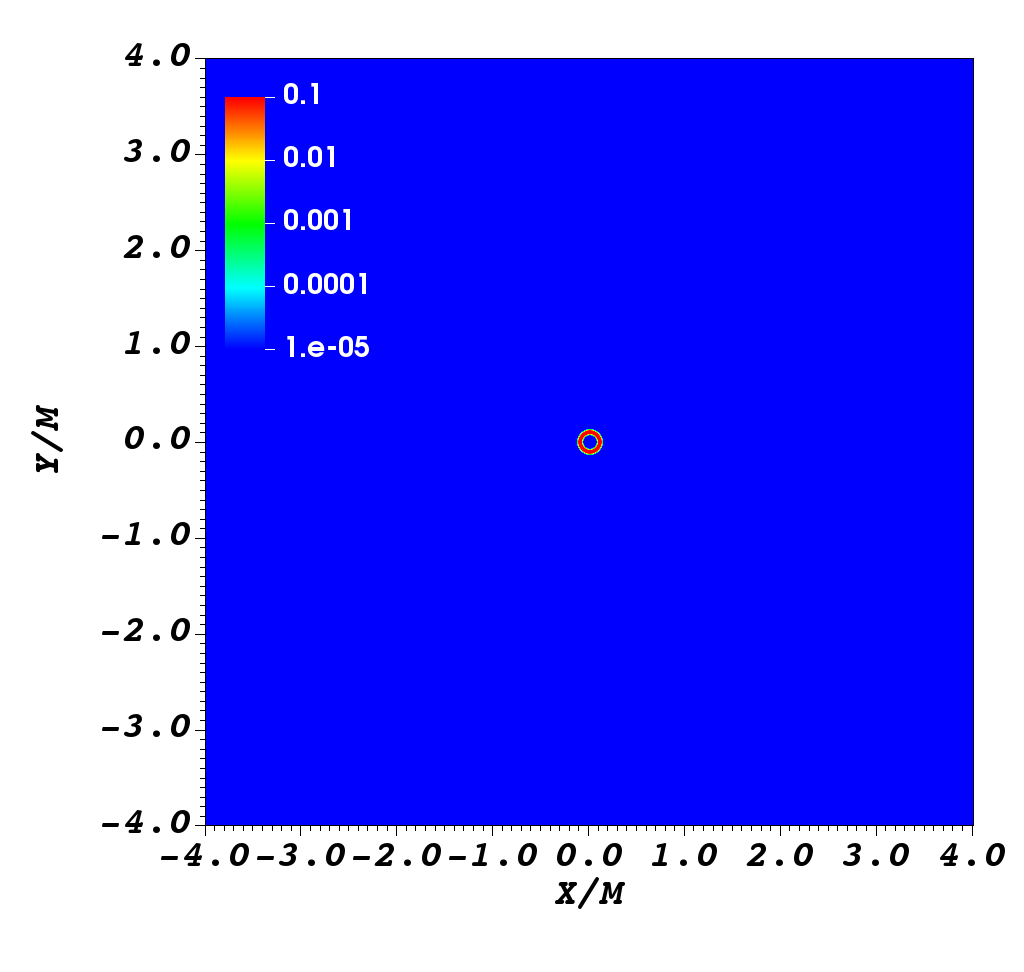
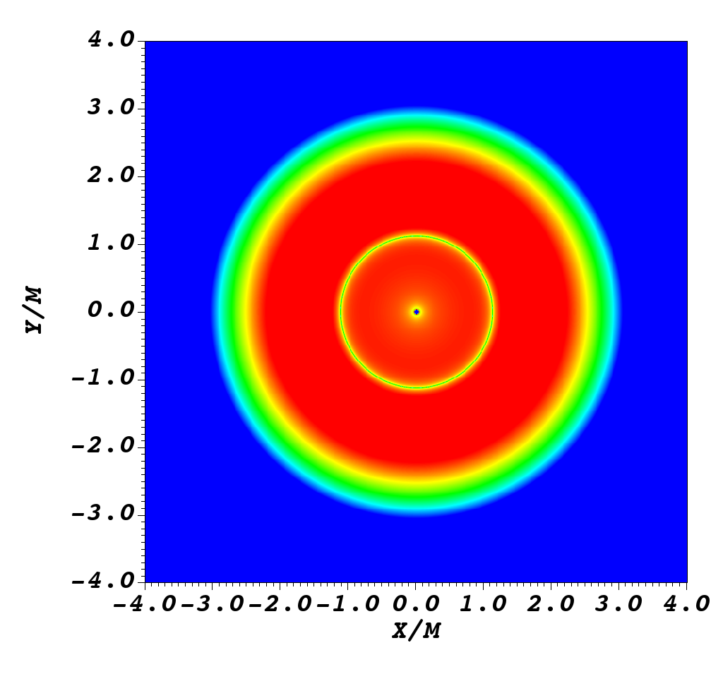
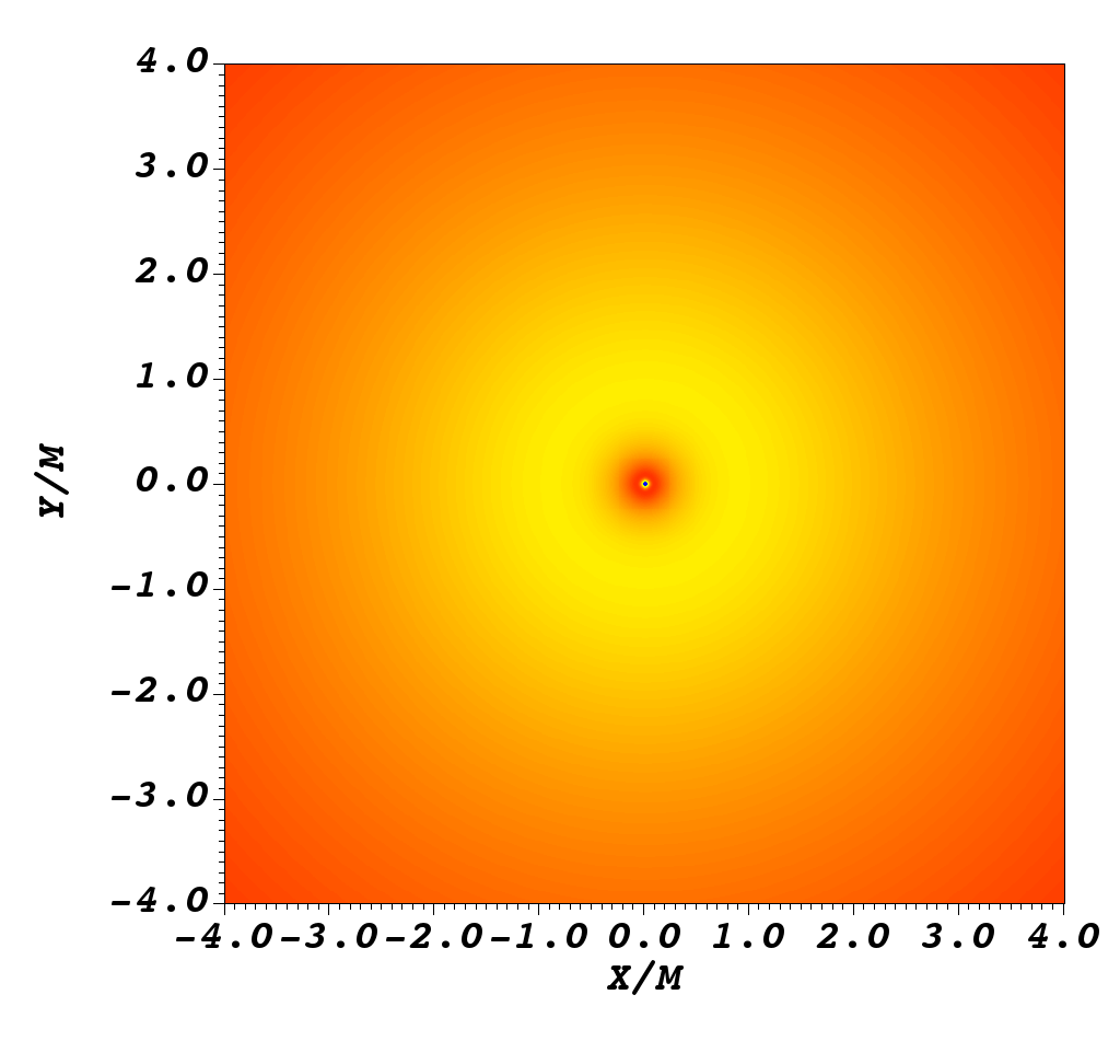
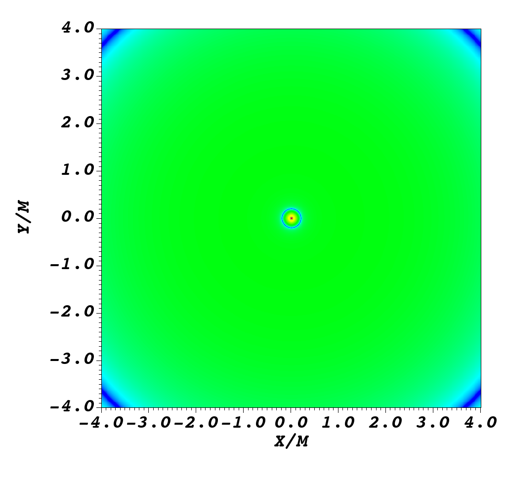
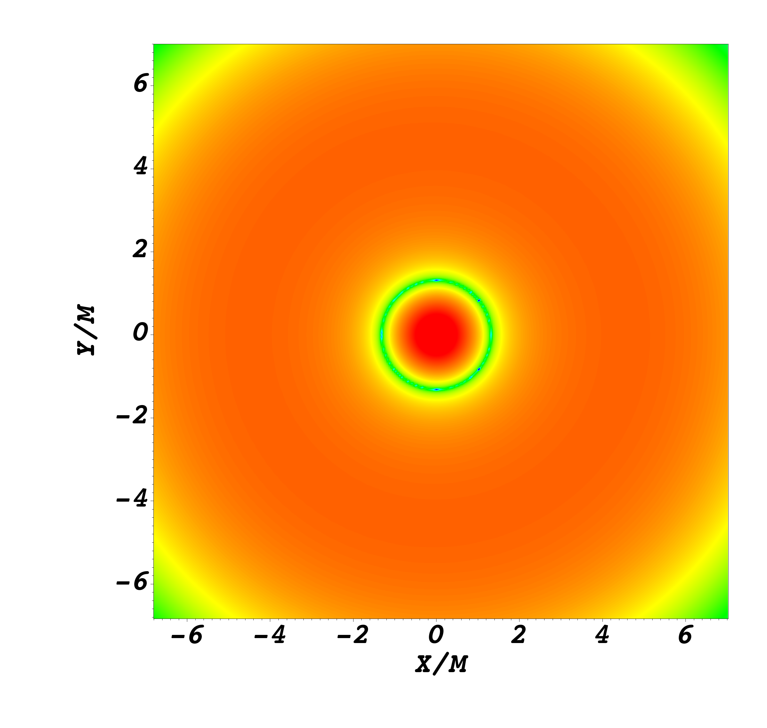
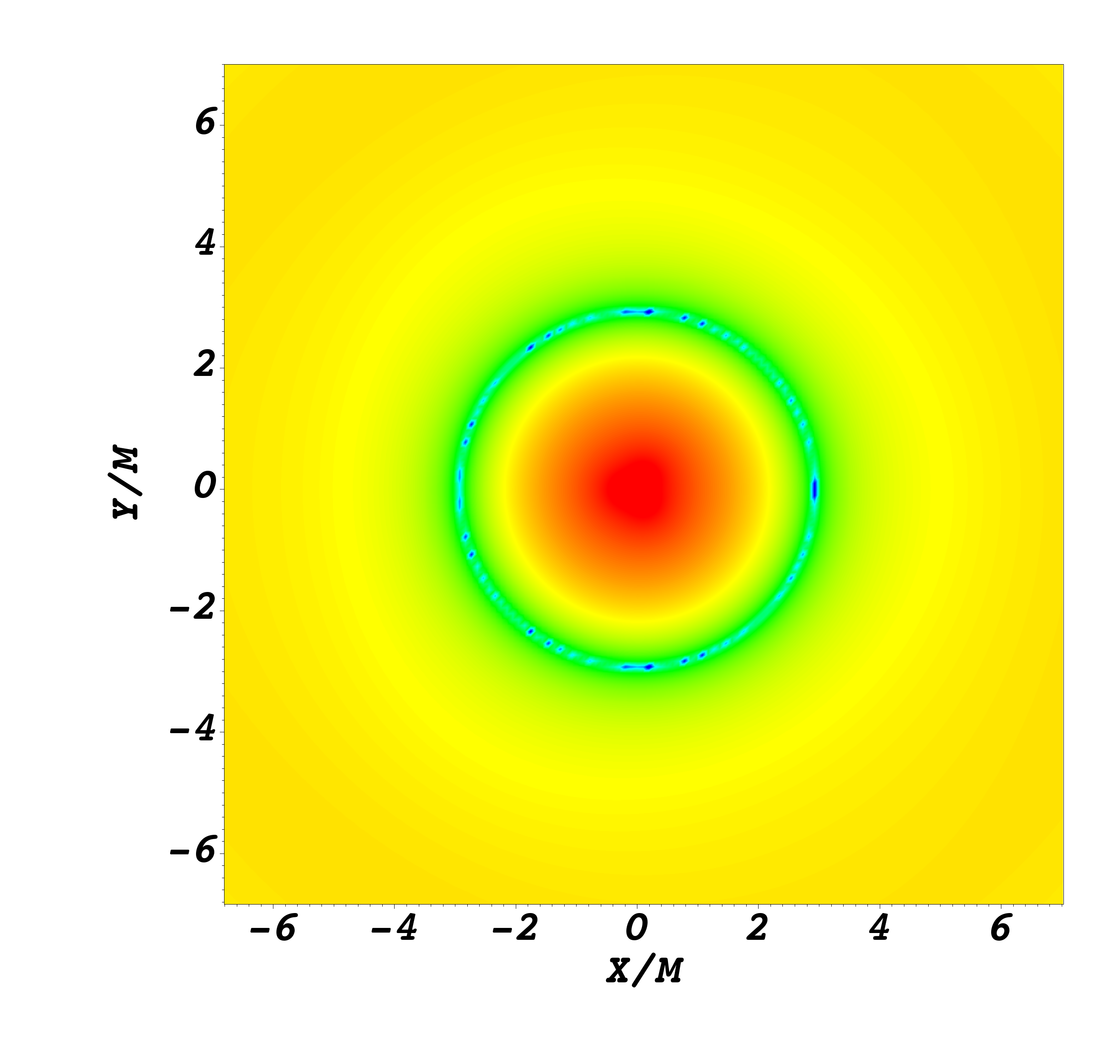
Figure 2: Snapshots of the evolution of a scalar field around the geometries depicted in Fig. 1 and studied in the following, namely: $4$-charge BH (top panel) corresponding to left panel in Fig. 3, an axisymmetric fuzzball (middle panel) corresponding to Fig. 5, and a $3$-center scaling microstate (bottom panel) corresponding to bottom panel in Fig. 7. From left to right, they are snapshots at $t/M=0,15,30,45,60$. Related movies are publicly available [92].

III.2 Numerical setup for time evolution

Here, we explain the numerical set up for the time evolution of a scalar field in a microstate geometry. Owing to its spherical symmetry, the case of a $4$-charge BH is much simpler and can be studied with a $1+1$ evolution code or in the frequency domain, as discussed in Appendix B. However, since the general fuzzball spacetime does not have spatial isometries, the field equation for the scalar field is not separable. We therefore evolve the scalar field using $3+1$ dimensional numerical simulations. The numerical implementation is based on the Einstein Toolkit infrastructure [93, 94, 95] with mesh refinement provided by the Carpet package [96, 97], and multipatch infrastructure provided by Llama [98]. The scalar field is evolved in the ScalarEvolve code, which has been previously used and tested in [99, 100, 101]. We implement a $4$-th order Runge-Kutta method, and the spatial derivatives are evaluated by $4$-th order finite differences. The buffer zones between different refinement levels are evaluated by using $5$-th order interpolation in space and $2$-nd order interpolation in time.

Compared to the standard case of fields evolving on a BH spacetime, more resolution layers are needed. Indeed, the fuzzball spacetime has high curvature regions around the centers which must be resolved during the evolution and, at the same time, the asymptotic behavior of the field must be accurately extracted at large distances in order to get the ringdown signal. Furthermore, although regular from the five dimensional perspective, four-dimensional fuzzball geometries are singular at the centers and such singular behavior should be regularized to perform stable numerical simulations. We regularize the geometry by replacing

$$\frac{1}{|\vec{x}-\vec{x}_{a}|}\to\frac{{\rm erf}(|\vec{x}-\vec{x}_{a}|/\epsilon)}{|\vec{x}-\vec{x}_{a}|}$$ (21)

in the harmonic functions $V$, $L_{I}$, $K^{I}$, and $W$. The error function smoothly interpolates between unity when $|\vec{x}-\vec{x}_{a}|\gg\epsilon$ and $\propto|\vec{x}-\vec{x}_{a}|$ when $|\vec{x}-\vec{x}_{a}|\ll\epsilon$. Furthermore, the expressions of the one-form $\omega$ has a coordinate singularity on the axis for axisymmetric fuzzball solutions (see Eq. (35)), which can be regularized by the following replacement:

$$\frac{1}{1-(\vec{n}_{a}\cdot\vec{n}_{ab})^{2}}\to\frac{1}{1-(\vec{n}_{a}\cdot\vec{n}_{ab})^{2}+\epsilon}\,.$$ (22)

Details about code testing and the regularization procedure of spacetime are given in Appendix C.

Concerning the initial data, we have performed a variety of simulations with different initial profiles. We report here two representative cases. The first type is a spherically symmetric Gaussian ‘shell’:

$$\Phi(0,x) = Ae^{-\left(\frac{r-r_{0}}{\sigma}\right)^{2}}\,,$$ (23)

whereas the second type is an $l=m=2$ profile:

$$\Phi(0,x) ={\cal W}(r,r_{\rm max},r_{\rm min}){\rm Re}(Y_{2,2}(\theta,\phi))\frac{r}{\sigma}e^{-\frac{r-r_{0}}{\sigma}}\,,$$ (24)

where $\sigma$ and $r_{0}$ define the typical width and central value location of the initial profile, and ${\cal W}(r)$ is a window function, which is a $5$-th order smooth polynomial satisfying ${\cal W}(r_{\rm min},r_{\rm max},r_{\rm min})=0$ and ${\cal W}(r_{\rm max},r_{\rm max},r_{\rm min})=1$. In both cases the initial scalar field is instantaneously static, i.e.

$$(\partial_{t}-\gamma^{i}\partial_{i})\Phi(0,x)=0\,,$$ (25)

where $\gamma^{i}$ is the shift vector in the $3+1$ decomposition of the metric [102].

IV Numerical Results

Here, we summarize the numerical results and discuss the scattering of a scalar wavepacket off fuzzball geometries. Figure 2 shows some representative snapshots of our simulations on the $y=0$ plane. Related movies are publicly available [92].

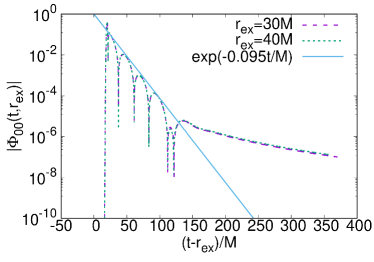
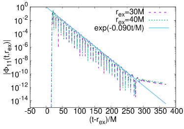
Figure 3: Time evolution of $(l,m)=(0,0)$ (left) and $(l,m)=(1,1)$ (right) multipole mode of a scalar field around a 4-charge BH solution with $(Q_{1}=Q_{3},Q_{2}=Q_{4})=(1.1,0.9)M$ at two different extraction radii. For the initial data, we took a instantaneously static Gaussian centered at $1.1M$ in tortoise coordinates and with width $\sigma=0.01M$ (see Appendix B). The general behavior is independent of the initial data.

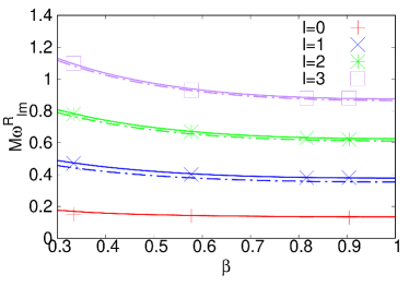
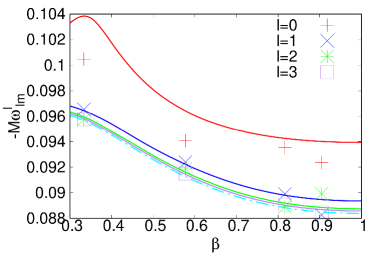
Figure 4: Real part (left panel) and imaginary part (right panel) of the fundamental QNMs of a $4$-charge BH with $Q_{1}=Q_{3}$ and $Q_{2}=Q_{4}=\beta^{2}Q_{1}$ as a function of $\beta$ for each $l$. Solid and dot-dashed curves refer to the exact frequency-domain computation (see Appendix B.2) and the analytical result of the geodesic analysis (see Eq. 18), respectively. Data points are the modes extracted from the time-domain waveform of our simulations.

IV.1 Ringdown of 4-charge BHs

We evolve the scalar field around a 4-charge BH with $Q_{1}=Q_{3}$ and $Q_{2}=Q_{4}$ based on the formulation discussed in Appendix B, and extract the field at fixed radius. Figure 3 shows the evolution of the scalar field with $l=0$ and $l=1$. We observe the standard QNM ringing, wherein the signal dies off exponentially until producing the typical late-time power-law tail due to backscattering off the gravitational potential [103]. Figure 4 shows the QNM frequency as a function of the single dimensionless parameter of the metric, $\beta=\sqrt{Q_{3}/Q_{1}}$, with $\beta\to 1$ being the extremal Reissner-Nordström limit. The data points in Fig. 4 are extracted from the simulations by fitting the time-domain waveform, whereas the dotted and solid curve respectively show the QNMs given by the analytical geodesic approximation [Eq.(18)] and by an exact frequency-domain code (see Appendix B.2). The analytical geodesic result is in excellent agreement with the exact one (especially for large $l$), and both are in good agreement with the results extracted from the time domain. The agreement of the imaginary part of the $l=0$ mode is less good (but still within a few percent) due to the smaller number of ringdown cycles before the power law (compare left and right panels of Fig. 3), which reduces the accuracy of the fit. Since the BH QNMs extracted from the time evolution are in good agreement with the photon sphere QNMs computed with the geodesic approximation, and since the latter are independent of the object interior, we expect the prompt ringdown to be described by the photon sphere modes also in the fuzzball case [57, 58]. In next subsection, we shall confirm this expectation and use it to distinguish the photon-sphere QNMs from other characteristic modes of the system.

IV.2 Ringdown and echoes of fuzzball microstates

Let us start by discussing the case of axisymmetric fuzzball solutions. Figure 5 shows the time evolution for initial data given in Eq. (23) with $\sigma=0.036M$ and $r_{0}=0$ around a $\kappa_{1}=\kappa_{2}=\kappa_{3}=\kappa=3$ axisymmetric fuzzball, taken as a representative example (the qualitative properties do not change for $\kappa>3$).

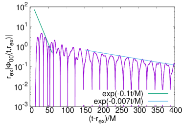
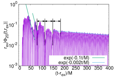
Figure 5: Time evolution of $l=m=0$ (left panel) and $l=2$, $m=0$ (right panel) multipole modes of the scalar field around axisymmetric fuzzball solution with $\kappa_{1}=\kappa_{2}=\kappa_{3}=\kappa=3$, and extracted at $r_{\rm ex}=23M$. The evolution starts from instantaneously static spherically symmetric Gaussian profile [Eq. (23)] with $\sigma=0.036M$ and $r_{0}=0$.

The absence of spherical symmetry produces mode mixing: the initially spherical profile excites both spherical ($l=m=0$) and quadrupolar ($l=2$, $m=0$) modes, where all dipolar ($l=1$) modes and the quadrupolar modes with $m\neq 0$ vanish identically due to the symmetries of the metric and to the angular momentum composition rules. Hexadecupolar ($l=4$, $m=0$) modes are also excited but are subleading and not shown in the plot.

In the prompt-ringdown phase of both modes, we observe the standard damped oscillations with a decay rate of about $0.1M$, in agreement with the geodesic result for the photon-sphere modes (see Table 1 and Fig. 4). At very late times, the decay is much slower and presumably corresponds to the long-lived QNMs of the fuzzball geometry. At intermediate times, we observe the typical echoes expected for horizonless geometries [57, 58, 72, 85, 86]. Echoes are more evident for the “induced” quadrupolar modes compared to the spherical mode. The reason for this is twofold: i) the effective potential for modes with large angular momentum is higher, so generically modes with larger $l$ are more efficiently confined; ii) the fuzzball’s gravitational potential has a quadrupolar component that can trap $l=2$ modes more efficiently, especially for mostly equatorial $l=m=2$ modes discussed below. Therefore, for spherical modes, echoes could be absent or possibly buried in the low-frequency fuzzball fundamental QNM that dominates the late response. For $l=2$, $m=0$, the typical time delay between echoes is roughly $\Delta t=35M$. Note, however, that it is difficult to identify accurately the echo delay time from the time evolution, especially due to the presence of multiple pulses. Indeed, our instantaneously static Gaussian pulse initially splits into an outgoing pulse and an ingoing pulse; the latter gets quickly reflected at $r=0$ and follows the outgoing pulse with a short delay [104], which is approximately $\Delta T\approx 16M$, as computed in the geodesic approximation for this solution. Therefore, we expect a complicate echo pattern from the modulation of this doublet.

Note also that the echo delay time in Fig. 5 cannot be directly compared with $\Delta t_{\pm}$ in Table 1, since the latter is valid for equatorial motion that corresponds to $l=m$ modes.  In order to perform such a comparison, in Fig. 6 we show the evolution starting from $l=2,m=2$ initial data [Eq. (24)].

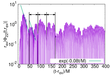
Figure 6: Same as in Fig. 5 but for the evolution of quadrupolar $l=m=2$ perturbations with initial data described by an instantaneously static $l=2,m=2$ Gaussian profile [Eq. (24)] with $\sigma=0.036M$, $r_{0}=0.14M$, $r_{\rm max}=0.07M$, and $r_{\rm min}=0.04M$. The extraction radius is $r_{\rm ex}=12M$. The prompt ringdown and the echo delay time are in agreement with the predictions in Table 1.

At early times, we observe the QNMs of the photon sphere (with a short decay time denoted by the green line), which is in good agreement with the estimation from the geodesic approximation and is indeed similar to the BH QNMs. After the prompt ringdown, the expected echo pattern appears. The delay time is highlighted by black arrows and is approximately $40M$, also in good agreement with the time scale predicted by the geodesic analysis. Some further interesting examples are presented in Appendix D.

We also note that the scaling of the delay time in the BH limit ($L\to 0$) might be very different for microstates of extremal (i.e., zero-temperature) BHs, as opposed to their finite temperature counterparts. For example, for the extremal Reissner-Nordstrom metric in the Schwarzschild-like coordinates (in which the horizon is at $r=M$), the light-crossing time near the surface $r=M(1+\delta)$ scales as $\Delta t_{+}\sim 1/\delta$, as opposed to the $\Delta t_{+}\sim\log(\delta)$ behavior in the subextremal case. Interestingly, for more realistic configurations at finite temperature we expect the delay time grows much more slowly than in our extremal case, facilitating the appearance of echoes.

Finally, let us focus on generic $3$-center microstate solutions. Although our method is general, for concreteness we focus on the scaling solution wherein the centers form an equilateral triangle (Fig. 1). This solution is equatorially symmetric but breaks axial symmetry so the geodesic approximation discussed in Sec. III.1 does not apply and we have to rely on numerical results only.

Figure 7 shows that the evolution of the scalar field starting from the spherically symmetric, instantaneously static, Gaussian initial data around two representative examples of scaling solution. The ringdown of this family of solutions shows the same qualitative features as in the axisymmetric case, in particular the echoes are more evident in the “induced” quadrupolar mode $l=2,\,m=0$, whereas the spherical mode displays immediately the long-lived, low-frequency fuzzball QNMs, that have a much longer decay time relative to the corresponding photon-sphere quantity. Although not shown, the evolution of $l=m=2$ initial data is similar to that presented in Fig. 6 for the axisymmetric solution.

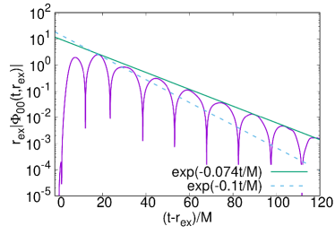
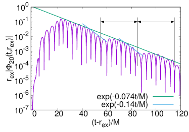
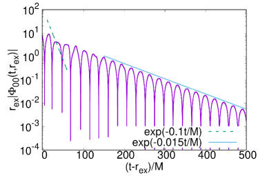
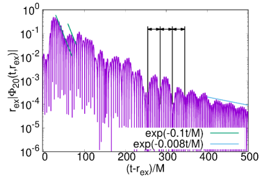
Figure 7: Time evolution of $l=0$ $m=0$ (left panel) and $l=2$, $m=0$ (right panel) multipole modes of the scalar field around scaling solution with $L=0.67M,\kappa=1$ (top panel), and $L=0.27M,\kappa=2$ (bottom panel). The evolution starts from instantaneously static spherically symmetric Gaussian profile [Eq.23] with $\sigma=0.67M$ (top panel) and $\sigma=0.27M$ (bottom panel). The extraction radius is $r_{\rm ex}=20.0M$ (top panel) and $r_{\rm ex}=8.0M$ (bottom panel)

V Discussion

We have developed a general technique to study the linear response of a large family of regular, horizonless fuzzball geometries describing the microstates of extremal spherically-symmetric BHs. These microstates do not possess spatial isometries, which makes the problem dramatically more involved than in the BH case.

For the first time, we studied the evolution of scalar perturbations on these geometries by using a $3+1$ numerical-relativity code. Our method is generic and can be applied to any stationary fuzzball. We unveiled the whole ringdown phenomenology studied in recent years for exotic compact objects [55, 56]; in particular, we showed that the prompt ringdown of fuzzballs is associated with the photon-sphere modes and mimics the BH response, whereas the presence of echoes [57, 58, 72, 85, 86] at late time is a smoking gun of some structure at the horizon scale and, in the particular model at hand, of the presence of the fuzzball’s regular throat.

We have performed several more simulations than those presented here and, in all cases, the perturbations always decay in time. Although our analysis was not systematic, it provides strong numerical evidence that the fuzzball microstates under consideration are linearly stable, at least until our maximum simulation time, $t\approx 1000M$. In addition, these geometries do not possess an ergoregion, so they are not plagued by the ergoregion instability of horizonless compact objects [105, 106, 107, 108, 109, 110, 111]. On the other hand, it has been argued that linear perturbations in certain microstate geometries (with an “evanescent” ergoregion) decay logarithmically in time and could be prone to instabilities at the nonlinear level [112] (see also [113, 114]). It would be interesting to check this result with numerical simulations for the solutions considered in this work.

Although in viable astrophysical scenarios BHs are expected to be neutral, charged BH solutions to supergravity are a useful toy model to explore the properties of their corresponding microstates. The numerical analysis developed here does not rely on supersymmetry and can be directly applied to putative non-supersymmetric and neutral microstates, should the latter be found. In this case, we expect that all the features found in this work will be qualitatively the same.

A natural extension of our work is to consider other types of perturbations. While adapting our code to study a test vector field or any self-interacting (possibly massive) test fields is straightforward, considering metric perturbations is technically possible but much more challenging, since in these charged geometries the perturbations of the metric, gauge fields, and scalar fields are coupled to each other. However, also in this case we expect that the salient features of the ringdown will remain qualitatively the same.

A more promising avenue could be to embed this family of microstate geometries into an effective model such as the one based on the membrane paradigm developed in [56]. Our results can be used to calibrate the model and check if it reproduces the salient features of the fuzzball ringdown phenomenology. An important missing ingredient in current models is the fact that – owing to the lack of spatial symmetries – different angular modes can be excited with comparable amplitude, even for highly symmetric initial data, as shown by our simulations.

On the longer run, the goal is to confront the predictions of the fuzzball scenario with gravitational-wave data, for example extending current ringdown tests [20, 56, 23] and echo searches [72, 73, 61, 74, 75, 76, 77, 78, 23] to include the predictions of this model, which are dramatically more complex than the toy models used so far to model gravitational-wave echoes.

On the theory side, our results also urge to address the “measure problem” with fuzzballs. As we have shown, in general the ringdown of a single microstate geometry is very peculiar and contains clear features that can be used to distinguish it from the standard BH ringdown. However, if a classical BH is described by a quantum superposition of microstates, then macroscopic observables (e.g. QNM frequencies and damping times) might be related to an average over the entire ensemble. Whether the signals should sum incoherently (possibly destroying the echo pattern) or what is the phase space and measure of this average remain open problems that should be urgently addressed if one wishes to test quantum-gravity effects near compact objects in the gravitational-wave era (see [115] for related discussion).

Studies of possible observational signatures of the fuzzball scenario are just in their infancy, but are acquiring considerable attention in the context of gravitational-wave and electromagnetic tests [51, 83, 49, 52, 116] (see [54] for a review) that may also encode string corrections [117, 118, 119] to memory effects [120]. We hope that our study on BH microstate spectroscopy could pave the way to further developments in this exciting field.

Appendix A Fuzzball microstate geometries

In this appendix we provide details on the fuzzball microstate geometries considered in the main text.

A.1 General multicenter fuzzball solutions

We are interested in solutions of the form (1) admitting a regular horizonless five-dimensional uplift with metric

$$ds_{5}^{2}=-(Z_{1}\,Z_{2}\,Z_{3})^{-{2\over 3}}\left[dt+\mu(d\Psi+w_{0})+w\right]^{2}+(Z_{1}\,Z_{2}\,Z_{3})^{1\over 3}\left[V^{-1}(d\Psi+w_{0})^{2}+Vd\vec{x}^{2}\right]$$ (26)

and $*_{3}dw_{0}=dV$. It can be seen that the resulting metric reduces to $\mathbb{R}$ times a Gibbons-Hawking space near the centers if $\mu$ vanishes and $Z_{I}$ remain finite near the centers. The origin of the Gibbons-Hawking space can display orbifold singularities if $|v_{a}|\neq 1$ but the latter can be easily regularized by splitting the centers (see [80] for a review). The finiteness of $Z_{I}$ is ensured by setting

$$\ell_{I,a}=-{1\over 2}\frac{|\epsilon_{IJK}|k_{a}^{J}k_{a}^{K}}{v_{a}}\,,\quad,\quad m_{a}=\frac{k_{a}^{1}k_{a}^{2}k_{a}^{3}}{v_{a}^{2}}$$ (27)

while the vanishing of $\mu$ leads to the so called “bubble equations” [80]

$$\sum_{b=1}^{N}\frac{\Gamma_{ab}}{r_{ab}}=\Lambda_{a}\,,$$ (28)

where $r_{ab}=|\vec{x}_{a}-\vec{x}_{b}|$,

$$\Gamma_{ab}=v_{a}v_{b}\prod_{I=1}^{3}\left(\frac{k_{a}^{I}}{v_{a}}-\frac{k_{b}^{I}}{v_{b}}\right)\qquad,\qquad\Lambda_{a}=\sum_{I=1}^{3}k_{a}^{I}-\frac{k_{a}^{1}k_{a}^{2}k_{a}^{3}}{v_{a}^{2}}\,.$$ (29)

Notice that Eq. (28) gives $N-1$ equations for the distances $r_{ab}$ and one equation for the coefficients $k_{a}^{I}$, namely

$$\sum_{a=1}^{N}\Lambda_{a}=0\,.$$ (30)

In order to remove singularities and closed time-like curves one should impose the following conditions

$$e^{2U}>0\,,\quad Z_{I}V>0\,.$$ (31)

Note that the first condition prevents the existence of an ergoregion and therefore these geometries are free of the ergoregion instability that exists for horizonless ultracompact objects [105, 106, 107, 108, 109, 110, 111] as well as for non-supersymmetric fuzzballs of the so-called JMaRT family [121, 122, 123].

The explicit expression for the one-form $\omega$ can be derived from Eq. (2) by making use of the bubble equations (28) and relations (27). One finds

$$\omega=\frac{1}{4}\sum_{a,b}^{N}\Gamma_{ab}\,\omega_{ab}\,,$$ (32)

with $\omega_{ab}=\vec{\omega}_{ab}{\cdot}d\vec{x}$ a solution of

$$\vec{\nabla}\times\vec{\omega}_{ab} = \frac{1}{|\vec{x}-\vec{x}_{a}|}\vec{\nabla}\frac{1}{|\vec{x}-\vec{x}_{b}|}-\frac{1}{|\vec{x}-\vec{x}_{b}|}\vec{\nabla}\frac{1}{|\vec{x}-\vec{x}_{a}|}\,.$$ (33)

The solution can be written as

$$\omega_{ab}=\frac{(\vec{n}_{a}+\vec{n}_{ab}){\cdot}(\vec{n}_{b}-\vec{n}_{ab})}{r_{ab}}\,d\phi_{ab}\,,$$ (34)

with

$$\vec{n}_{a}=\frac{\vec{x}-\vec{x}_{a}}{|\vec{x}-\vec{x}_{a}|}\,,\quad\vec{n}_{ab}=\frac{\vec{x}_{a}-\vec{x}_{b}}{r_{ab}}\,,\quad d\phi_{ab}=\frac{(\vec{n}_{a}\times\vec{n}_{ab})\cdot d\vec{x}}{|\vec{x}-\vec{x}_{a}|\left[1-(\vec{n}_{a}\cdot\vec{n}_{ab})^{2}\right]}\,.$$ (35)

The solution carry in general four electric, $Q_{A}=(Q_{0},Q_{I})$, and four magnetic, $P_{A}=(P^{0},P^{I})$, charges respectively given by

$$P^{0} = \sum_{a}v_{a}\quad,\quad Q_{I}=\sum_{a}\ell_{I,a}=-{1\over 2}\sum_{a}\frac{|\epsilon_{IJK}|k_{a}^{J}k_{a}^{K}}{v_{a}}\,,$$

$$P^{I} = \sum_{a}k^{I}_{a}\quad,\quad Q_{0}=\sum_{a}m_{a}=\sum_{a}\frac{k_{a}^{1}k_{a}^{2}k_{a}^{3}}{v_{a}^{2}}\,.$$ (36)

A.2 Axisymmetric three-center solutions with $v_{a}\neq 1$

We consider first a family of axisymmetric solutions with equatorial symmetry $z\to-z$ ($\theta\to\pi-\theta)$ . We align the three centers along the $z$-axis

$$\vec{x}_{a} =(0,0,z_{a})\quad,\quad z_{1}=L\qquad,\qquad z_{2}=0\qquad,\qquad z_{3}=-L\,,$$ (37)

and take the charges to be

$$v_{1} =v_{3}=-1\quad,\quad v_{2}=3\quad,\quad k^{I}{}_{a} =\left(\begin{array}[]{ccc}-\kappa_{1}&~{}~{}0{}{}&\kappa_{1}\\ -\kappa_{2}&~{}~{}0{}{}&\kappa_{2}\\ -\kappa_{3}&~{}~{}0{}{}&\kappa_{3}\\ \end{array}\right)$$ (38)

This is therefore a $3$-parameter family of solutions spanned by the integers $\kappa_{1}$, $\kappa_{2}$, and $\kappa_{3}$. For this case, $\Gamma_{ab}$ and $\Lambda_{a}$ take the simple form

$$\Gamma_{ab} =\kappa_{1}\kappa_{2}\kappa_{3}\left(\begin{array}[]{ccc}0&-{v_{2}\over v_{1}^{2}}&-{8\over v_{1}}\\ {v_{2}\over v_{1}^{2}}&~{}~{}0{}{}&-{v_{2}\over v_{1}^{2}}\\ {8\over v_{1}}&{v_{2}\over v_{1}^{2}}&0\\ \end{array}\right)\qquad,\qquad\Lambda_{a}=\kappa_{1}\kappa_{2}\kappa_{3}\left(\begin{array}[]{c}-{{q}}+{1\over v_{1}^{2}}\\ 0\\ {{q}}-{1\over v_{1}^{2}}\\ \end{array}\right)\,,$$ (39)

with ${{q}}={\kappa_{1}+\kappa_{2}+\kappa_{3}\over\kappa_{1}\kappa_{2}\kappa_{3}}$. The bubble equations are solved for

$$L={4\,v_{1}+v_{2}\over{{q}}\,v_{1}^{2}-1}\,,$$ (40)

whereas the one-form $\omega=\omega_{\phi}d\phi$ takes the form

$$\omega_{\phi}=\sum_{b>a}^{N}\frac{\Gamma_{ab}}{2r_{a}r_{b}\left(z_{a}-z_{b}\right)}\left[\left(r_{a}+z_{a}-r\cos\theta\right)\left(r_{b}-z_{b}+r\cos\theta\right)-r^{2}\sin^{2}\theta\right]$$ (41)

with $N=3$ and

$$r_{a}=|\vec{x}-\vec{x}_{a}|\,,$$ (42)

so that

$$r_{1}^{2}=r^{2}+L^{2}-2\,r\,L\,\cos\theta\quad,\quad r^{2}_{2}=r^{2}\quad,\quad r_{3}^{2}=r^{2}+L^{2}+2\,r\,L\,\cos\theta\,.$$ (43)

For completeness, we list the harmonic functions and other relevant quantities. The eight harmonic functions are

$$V=1+v_{1}\left[\frac{1}{r_{1}}+\frac{1}{r_{3}}\right]+\frac{v_{2}}{r_{2}}\quad,\quad W=\frac{\kappa_{1}\kappa_{2}\kappa_{3}}{v_{1}^{2}}\left[-\frac{1}{r_{1}}+\frac{1}{r_{3}}\right]$$ (44)

$$L_{1}=1{-}\frac{\kappa_{2}\kappa_{3}}{v_{1}}\left[\frac{1}{r_{1}}{+}\frac{1}{r_{3}}\right]\quad,\quad L_{2}=1{-}\frac{\kappa_{1}\kappa_{3}}{v_{1}}\left[\frac{1}{r_{1}}+\frac{1}{r_{3}}\right]\quad,\quad L_{3}=1{-}\frac{\kappa_{1}\kappa_{2}}{v_{1}}\left[\frac{1}{r_{1}}{+}\frac{1}{r_{3}}\right]$$

$$K_{1}={-}\kappa_{1}\left[\frac{1}{r_{1}}{-}\frac{1}{r_{3}}\right]\quad,\quad K_{2}=\kappa_{2}\left[{-}\frac{1}{r_{1}}{+}\frac{1}{r_{3}}\right]\quad,\quad K_{3}=\kappa_{3}\left[-\frac{1}{r_{1}}{+}\frac{1}{r_{3}}\right]\,.$$

The nonvanishing charges are (remind $v_{1}=v_{3}=-1,v_{2}=3$)

$$P^{0}=2v_{1}+v_{2}\quad,\quad Q_{1}=-\frac{2\kappa_{2}\kappa_{3}}{v_{1}}\quad,\quad Q_{2}=-\frac{2\kappa_{1}\kappa_{3}}{v_{1}}\quad,\quad Q_{3}=-\frac{2\kappa_{1}\kappa_{2}}{v_{1}}$$ (45)

To ensure that the charges are positive, we assume

$$\kappa_{1},\kappa_{2},\kappa_{3}\geq 1\quad,\quad v_{1}<0\quad,\quad v_{2}+2v_{1}>0\,.$$ (46)

The mass $M$ and entropy $S$ of the corresponding BH read

$$M =\frac{P^{0}{+}Q_{1}{+}Q_{2}{+}Q_{3}}{4}=\frac{v_{1}(v_{2}+2v_{1})-2(\kappa_{1}\kappa_{2}+\kappa_{2}\kappa_{3}+\kappa_{1}\kappa_{3})}{4v_{1}}\,,$$ (47)

$$S^{2} \propto\lim_{r\to 0}r^{4}e^{-4U}=-(v_{2}+2v_{1})\frac{8\kappa_{1}^{2}\kappa_{2}^{2}\kappa_{3}^{2}}{v_{1}^{3}}\,,$$

and are positive by construction. The total angular momentum of the solution reads $\vec{J}=J\vec{e}_{z}$, with

$$J=-\kappa_{1}\kappa_{2}\kappa_{3}{4v_{1}+v_{2}\over 2v_{1}^{2}}.$$ (48)

Notice that under the following scaling

$$v_{a}\to\gamma v_{a}\quad,\quad\kappa_{i}\to\gamma\kappa_{i}\,,$$ (49)

all the charges scale as

$$Q_{I}\to\gamma Q_{I}\quad,\quad P^{0}\to\gamma P^{0}\quad,\quad M\to\gamma M\quad,\quad J\to\gamma^{2}J\quad,\quad S\to\gamma^{2}S\,.$$ (50)

This is an overall scaling, therefore dimensionless quantities such as $M\omega_{\rm QNM}$ are not affected by it. This implies that any given solution can be scaled to a solution with arbitrarily large charges and mass.

Finally, the $4$-charge BH associated to the fuzzball solution is obtained by bringing the three centers to the origin. In this case harmonic functions become

$$V=1+\frac{v_{2}+2v_{1}}{r}\quad,\quad L_{1}=1{+}\frac{2\kappa_{2}\kappa_{3}}{v_{1}r}\quad,\quad L_{2}=1{+}\frac{2\kappa_{1}\kappa_{3}}{v_{1}r}\quad,\quad L_{3}=1{+}\frac{2\kappa_{1}\kappa_{2}}{v_{1}r}$$ (51)

$$K^{I}={{W}}=0\,,$$

leading to

$$e^{-4U} =L_{1}L_{2}L_{3}V\qquad,\qquad\omega=0$$ (52)

The mass, charges, and entropy are given by Eqs. (45)-(47), whereas the BH is nonspinning, $J=0$.

A.3 Three-center solutions with $v_{a}=1$

The second family of solutions we consider are those with three centers, $v_{a}=1$ and four charges $Q_{0}=P^{I}=0$. The general solution to the bubble equation is described by four integers $\kappa_{a}$ specifying the $k_{a}^{I}$-matrix to be of the form

$$k^{I}{}_{a}=\left(\begin{array}[]{ccc}-\kappa_{1}\kappa_{2}&-\kappa_{1}\kappa_{3}&\kappa_{1}(\kappa_{2}+\kappa_{3})\\ \kappa_{3}&\kappa_{2}&-\kappa_{2}-\kappa_{3}\\ -\kappa_{4}&\kappa_{4}&0\\ \end{array}\right).$$ (53)

and therefore

$$V =1+\sum_{a=1}^{3}{1\over r_{a}}\,,\quad{{W}}=\kappa_{1}\,\kappa_{2}\,\kappa_{3}\,\kappa_{4}\left({1\over r_{1}}-{1\over r_{2}}\right)$$ (54)

$$L_{1} =1+\kappa_{4}\left({\kappa_{3}\over r_{1}}-{\kappa_{2}\over r_{2}}\right)\,,\quad L_{2}=1+\kappa_{1}\kappa_{4}\left(-{\kappa_{2}\over r_{1}}+{\kappa_{3}\over r_{2}}\right)$$

$$L_{3} =1+\kappa_{1}\left({\kappa_{2}\kappa_{3}\over r_{1}}+{\kappa_{2}\kappa_{3}\over r_{2}}+{(\kappa_{2}+\kappa_{3})^{2}\over r_{3}}\right)\,,\quad K^{1}=\kappa_{1}\left(-{\kappa_{2}\over r_{1}}-{\kappa_{3}\over r_{2}}+{\kappa_{2}+\kappa_{3}\over r_{3}}\right)$$

$$K^{2} ={\kappa_{3}\over r_{1}}+{\kappa_{2}\over r_{2}}-{\kappa_{2}+\kappa_{3}\over r_{3}}\,,\quad K^{3}=\kappa_{4}\left(-{1\over r_{1}}+{1\over r_{2}}\right)$$

again with $r_{a}=|\vec{x}-\vec{x}_{a}|$ and $\kappa_{i}$ some arbitrary integers. The solution describes a microstate of a Reissner-Nordström BH with a magnetic charge $P^{0}$ and three electric charges $Q_{I}$ given by

$$P^{0}{\,=\,}3\quad,\quad Q_{1}{\,=\,}\kappa_{4}(\kappa_{3}{\,-\,}\kappa_{2})\quad,\quad Q_{2}{\,=\,}\kappa_{1}\kappa_{4}(\kappa_{3}{\,-\,}\kappa_{2})\quad,\quad Q_{3}{\,=\,}\kappa_{1}(\kappa_{2}^{2}{\,+\,}4\kappa_{2}\kappa_{3}{\,+\,}\kappa_{3}^{2})\,.\\$$ (55)

The bubble equations constrain the distances $r_{ab}=|\vec{x}_{a}-\vec{x}_{b}|$ between the centers to be related by

$$r_{12} = \frac{2\kappa_{1}\kappa_{4}(\kappa_{2}-\kappa_{3})^{2}r_{23}}{\kappa_{1}\kappa_{4}(2\kappa_{2}^{2}+5\kappa_{2}\kappa_{3}+2\kappa_{3}^{2})+(\kappa_{2}+\kappa_{4}-\kappa_{1}\kappa_{3}+\kappa_{1}\kappa_{2}\kappa_{3}\kappa_{4})r_{23}}$$

$$r_{13} = \frac{\kappa_{1}\kappa_{4}(2\kappa_{2}+\kappa_{3})(\kappa_{2}+2\kappa_{3})r_{23}}{\kappa_{1}\kappa_{4}(2\kappa_{2}^{2}+5\kappa_{2}\kappa_{3}+2\kappa_{3}^{2})-(\kappa_{1}-1)(\kappa_{2}+\kappa_{3})r_{23}}.$$ (56)

A.3.1 Scaling solution

The simplest solution in this class is the so-called scaling solution, corresponding to the choice

$$\kappa_{1}=1\qquad,\qquad\kappa_{2}=0\qquad,\qquad\kappa_{3}=\kappa_{4}=\kappa\,.$$ (57)

For this choice one finds

$$P^{0}= \,3\quad,\quad Q_{I}=(\kappa^{2},\kappa^{2},\kappa^{2})\quad,\quad M=\frac{3(1{\,+\,}\kappa^{2})}{4}\quad,\quad J=0\,.$$ (58)

In particular, note that the solution is non-spinning. The centers are located at the vertices of an equilateral triangle.

$$(x_{1},y_{1},z_{1}) = \left(\frac{L}{2\sqrt{3}},\frac{L}{2},0\right)\,,\quad\quad(x_{2},y_{2},z_{2})=\left(\frac{L}{2\sqrt{3}},-\frac{L}{2},0\right)\quad,\quad(x_{3},y_{3},z_{3})=\left(-\frac{L}{\sqrt{3}},0,0\right)\,.$$ (59)

A.3.2 Another axisymmetric solution

Although not considered in the main text, for completeness we provide here another axisymmetric solution. In this case axial symmetry is found for the choice $\kappa_{2}=0$ and $\kappa_{4}=\kappa_{1}\kappa_{3}$, i.e.

$$k^{I}{}_{a}=\kappa_{3}\left(\begin{array}[]{ccc}0&-\kappa_{1}&\kappa_{1}\\ 1&0&-1\\ -\kappa_{1}&\kappa_{1}&0\\ \end{array}\right)\,.$$ (60)

The centers are located at

$$\vec{x}_{a}=(0,0,z_{a})\quad,\quad z_{1}=L\qquad,\qquad z_{2}=0\qquad,\qquad z_{3}=-L\,,$$ (61)

with

$$L=\frac{\kappa_{1}^{2}\kappa_{3}^{2}}{\kappa_{1}-1}\,.$$ (62)

The mass, charges, angular momentum and entropy of the solution read

$$P^{0} =3\,,\quad Q_{1}{\,=\,}\kappa_{1}\kappa_{3}^{2}\,,\quad Q_{2}{\,=\,}\kappa_{1}^{2}\kappa_{3}^{2}\,,\quad Q_{3}{\,=\,}\kappa_{1}\kappa_{3}^{2}\,,$$ (63)

$$M =\frac{3+\kappa_{1}\kappa_{3}^{2}(2+\kappa_{3})}{4}\,,\quad\vec{J}=-\frac{1}{2}\kappa_{1}^{2}\kappa_{3}^{3}\,\vec{e}_{z}\qquad,\qquad S=3\kappa_{1}^{4}\kappa_{3}^{6}\,.$$

Appendix B Numerical implementation for 4-charge BH

B.1 Time-domain analysis

To evolve the scalar field in a spherically symmetric BH, it is convenient to define an effective potential for different angular modes. The isotropic coordinates in Eq. (7) can be transformed into areal radius coordinates as:

$$ds^{2} =-f(r)dt^{2}+g(r)\left(\frac{2{{\varrho}}}{r^{2}g^{\prime}(r)+2rg(r)}\right)^{2}d{{\varrho}}^{2}+{{\varrho}}^{2}d^{2}\Omega\,,$$ (64)

where ${{\varrho}}^{2}=g(r)r^{2}$. In the general case of four independent charges, the analytical expression for ${{\varrho}}(r)$ is cumbersome. If we assume $Q_{1}=Q_{3}$ and $Q_{2}=Q_{4}$ for simplicity, then the horizon areal radius is ${{\varrho}}_{\rm H}=\sqrt{Q_{1}Q_{2}}$, and the metric reduces to

$$ds^{2}=-{{B}}({{\varrho}})^{2}dt^{2}+{{A}}({{\varrho}})^{2}d{{\varrho}}^{2}+{{\varrho}}^{2}d^{2}\Omega\,,$$ (65)

where

$${{B}}({{\varrho}}) = \frac{\sqrt{(Q_{1}-Q_{2})^{2}+4{{\varrho}}^{2}}-(Q_{1}+Q_{2})}{2{{\varrho}}}\,,$$

$${{A}}({{\varrho}}) = \frac{4{{\varrho}}^{2}}{(Q_{1}-Q_{2})^{2}+4{{\varrho}}^{2}-(Q_{1}+Q_{2})\sqrt{(Q_{1}-Q_{2})^{2}+4{{\varrho}}^{2}}}\,.$$

Since the space-time is spherically symmetric, we can separate the angular dependence of the field as

$$\Phi = \sum_{l,m}\frac{\sigma_{lm}(t,{{\varrho}})}{{{\varrho}}}Y_{lm}(\theta,\phi)\,,$$ (67)

where $Y_{lm}(\theta,\phi)$ are the spherical harmonics. The tortoise coordinate ${{\varrho}}_{\ast}$ is defined as $\frac{d{{\varrho}}_{\ast}}{d{{\varrho}}}=\frac{{{A}}}{{{B}}}$, which yields

$${{\varrho}}_{\ast}= \frac{1}{2}\sqrt{(Q_{1}-Q_{2})^{2}+4{{\varrho}}^{2}}+\frac{2Q_{1}Q_{2}}{Q_{1}+Q_{2}-\sqrt{(Q_{1}-Q_{2})^{2}+4{{\varrho}}^{2}}} +(Q_{1}+Q_{2})\ln\left(Q_{1}+Q_{2}-\sqrt{(Q_{1}-Q_{2})^{2}+4{{\varrho}}^{2}}\right)\,.$$ (68)

Finally, the evolution equation for $\sigma_{lm}(t,R)$ in tortoise coordinates is governed by

$$-\frac{\partial^{2}}{\partial t^{2}}\sigma_{lm}+\frac{\partial^{2}}{\partial{{\varrho}}_{\ast}^{2}}\sigma_{lm}-V_{\rm eff}({{\varrho}})\sigma_{lm}=0$$ (69)

where the effective potential reads

$$V_{\rm eff}({{\varrho}}_{\ast}) ={{B}}^{2}\left(\frac{l(l+1)}{{{\varrho}}^{2}}+\frac{1}{{{\varrho}}{{A}}^{2}}\left(\frac{\partial_{{{\varrho}}}{{B}}}{{{B}}}-\frac{\partial_{{{\varrho}}}{{A}}}{{{A}}}\right)\right)\,.$$ (70)

We integrate Eq. (69) numerically with an ingoing boundary condition at ${{\varrho}}_{\ast}\to-\infty$ (i.e., $\partial_{t}\sigma_{lm}\sim\partial_{{{\varrho}}_{\ast}}\sigma_{lm}$), and outgoing boundary condition at ${{\varrho}}_{\ast}\to\infty$ (i.e., $\partial_{t}\sigma_{lm}\sim-\partial_{{{\varrho}}_{\ast}}\sigma_{lm}$).

For the initial data for simulation we choose an instantaneously static Gaussian initial data,

$$\sigma_{lm}(0,{{\varrho}}_{\ast}) = {{a}}e^{-\left(\frac{{{\varrho}}_{\ast}-{{\varrho}}_{0}}{\sigma}\right)^{2}}\,,$$ (71)

$$\dot{\sigma}_{lm}(0,{{\varrho}}_{\ast}) = 0\,,$$ (72)

where ${{a}}$, ${{\varrho}}_{0}$, and $\sigma$ are the initial amplitude, position, and width of the Gaussian pulse, respectively. Note that our initial data are given for each $(l,m)$ mode separately, since the modes are decoupled in the spherically symmetric background. We used a C++ numerical code to integrate Eq. (69) using a 4th-order Runge-Kutta method, where spatial derivatives are evaluated by 4th-order finite difference.

B.2 Frequency-domain analysis

In the spherically-symmetric case it is straightforward to integrate the Klein-Gordon equation as an eigenvalue problem in order to compute directly the QNMs of the $4$-charge BH.

In the particular case $Q_{1}=Q_{3}$ and $Q_{2}=Q_{4}$, Eq. (69) reduces to a single ordinary differential equation in a Schroedinger-like form by assuming $\sigma_{lm}=\Psi(\varrho)e^{-i\omega t}$. Boundary conditions are then imposed ($\Psi\to e^{\pm i\omega{\varrho_{\ast}}}$ as $\varrho_{\ast}\to\pm\infty$) in order to compute the complex eigenvalues $\omega$. In the general case, $r^{4}_{H}=Q_{1}Q_{2}Q_{3}Q_{4}$, the same method can be implemented by integrating the Klein-Gordon equation on the metric (7) using directly isotropic coordinates. By decomposing the field as $\Phi=\sum_{lm}\frac{{{F}}(r)}{r}Y_{lm}e^{-i\omega t}$, the Klein-Gordon equation takes a particularly simple form,

$${{F}}^{\prime\prime}+\left(\omega^{2}\frac{(Q_{1}+r)(Q_{2}+r)(Q_{3}+r)(Q_{4}+r)}{r^{4}}-\frac{l(l+1)}{r^{2}}\right){{F}}=0\,.$$ (73)

In both cases, we computed the fundamental eigenfrequencies $\omega$ using an extended version of the direct integration method [124, 125]. Following [126], the QNMs can also be found ‘analytically’ by means of the ‘quantum’ Seiberg-Witten curve of ${\cal N}=2$ super Yang-Mills theory with $SU(2)$ gauge group and RG-invariant scale $\Lambda$, coupled to $N_{f}=2$ hypermultiplet doublets with masses $m_{1,2}$, after the identifications ${\Lambda}=+2i\hbar\omega r_{H}$, ${m_{1}}={\hbar\over 2}-2i\hbar\omega\sum_{A}Q_{A}$, ${m_{2}}=-{\hbar\over 2}-2i\hbar\omega\sum_{A}{r_{H}^{2}\over Q_{A}}$ and ${u}=\hbar^{2}\left[(l+{1\over 2})^{2}+\omega^{2}(2r_{H}^{2}-\sum_{A<B}Q_{A}Q_{B})\right]$ [127].

Appendix C Code tests and regularization procedure for fuzzball simulations

In this appendix we provide some technical details of our code. First of all, since microstate geometries are cumbersome, it is useful to check the analytical solutions. For this purpose, in the left panel of Fig. 8, we check the numerical convergence of residual in the differential form of Eq. (2) for different resolutions. The residual shows convergence with fourth-order accuracy, as expected since the spatial derivatives are evaluated by fourth-order-accurate finite difference stencils.

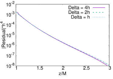
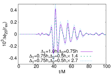
Figure 8: Convergence of the residual of the differential form in Eq. (2) on $z$-axis for different resolutions $h$ (left panel), and convergence analysis of the $l=2$, $m=0$ multipole mode of the scalar field at $r_{\rm ex}=20M/3$ (right panel).

The right panel of Fig. 8 shows the evolution of the difference $\Delta\Phi_{20}$ between the field $\Phi_{20}$ at different resolutions $\Delta_{1}$ and $\Delta_{2}$ for a simulation starting from instantaneously static Gaussian initial data with $\sigma=0.33M$ around the microstate scaling solution with $\kappa=1$, and $L=0.67M$. In our code, the spatial derivatives are approximated with fourth-order-accurate finite difference stencils, and the time integration is performed by a 4th-order Runge-Kutta method. The boundary of the mesh refinement boundary is interpolated with second order and fifth order accuracy in time and space. We define the convergence factor

$$Q_{n}=\frac{\Phi_{20}(\Delta_{c})-\Phi_{20}(\Delta_{m})}{\Phi_{20}(\Delta_{m})-\Phi_{20}(\Delta_{h})}=\frac{\Delta_{c}^{n}-\Delta_{m}^{n}}{\Delta_{m}^{n}-\Delta_{h}^{n}}\,,$$ (74)

where $\Delta_{c}=\Delta$, $\Delta_{m}=0.75\Delta$, $\Delta_{h}=0.5\Delta$, and $n$ is expected convergence factor. As shown in the right panel of Fig. 8 the numerical evolutions converge between second- and third-order accuracy, as expected.

Finally, we discuss the regularization procedure to resolve the singularities of the $4$-dimensional fuzzball geometry near the centers. In Fig. 9 we show an example of evolution for different values of the regularization parameter $\epsilon$. While the initial response is independent of $\epsilon$ – since it is related to the properties of the photon sphere and not to the region near the centers – the behavior at later times depends on $\epsilon$ if the latter parameter is not sufficiently small. The two smallest values of $\epsilon$ give the same evolution for $l=0$, whereas small finite-$\epsilon$ differences arise at late times for $l=2$. Such differences become smaller as $\epsilon\to 0$ and, anyway, do not affect the overall structure of the signal. While using even smaller values of $\epsilon$ is computationally very expensive, our simulations indicate that for sufficiently small $\epsilon$ the evolution is regular and smoothly convergent.

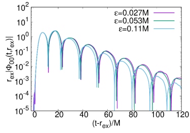
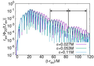
Figure 9: Time evolution of $l=0$ $m=0$ (left panel) and $l=2$, $m=0$ (right panel) multipole modes of the scalar field around scaling solution with $L=0.67M,\kappa=1$. The evolution starts from instantaneously static spherically symmetric Gaussian profile Eq.23 with $\sigma=0.33M$. The extraction radius is $r_{\rm ex}=20.0M$.

Note also that the singularities at the centers are problematic only if they coincide with some of the numerical grid points, otherwise a natural cut-off is set by the grid numerical resolution. We have adopted this strategy to probe much smaller values of the cut-off, confirming the generic behavior discussed above, although for very small values of the cut-off reaching numerical convergence requires very high resolution.

Appendix D Extra simulations

For completeness, in this appendix we consider two further examples of evolution in the axisymmetric microstate geometry with $\kappa_{1}=\kappa_{2}=\kappa_{3}=\kappa$. In particular, in the left and right panels of Fig. 10 we consider the evolution of the $l=m=2$ initial data on a solution with $\kappa=2$ and $\kappa=4$, respectively. The former case is interesting because, according to our geodesic analysis, it does not possess a light ring on the equatorial plane. Correspondingly, we do not observe echoes in this case since radiation confined near the equator cannot be efficiently trapped. On the other hand, the standard prompt ringdown shown in the left panel could be identified with a nontrivial geodesic structure outside the equatorial plane for this geometry. Finally, in the case $\kappa=4$ there is an equatorial light ring which can efficiently confine radiation. Furthermore, in this case the fuzzball’s throat is deeper and the associated echo delay time is about $64M$ (see Table 1). This is in qualitative agreement with the timescales shown in the right panel of Fig. 10, confirming that the physical picture drawn from the geodesics approximation is reliable.

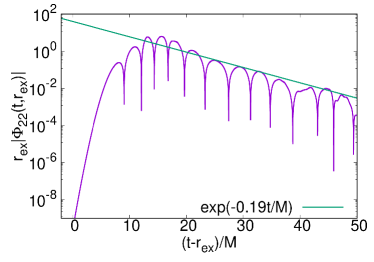
Figure 10: Evolution of an instantaneously static $l=m=2$ initial Gaussian profile on the axisymmetric microstate geometry with $\kappa_{1}=\kappa_{2}=\kappa_{3}=\kappa$. Left panel: $\kappa=2$; in this case the absence of an equatorial light ring implies the absence of echoes at late time. Right panel: $\kappa=4$; also in this case the echo delay time is consistent with the geodesics prediction in Table 1.

References

- [1] B. Carter, “Axisymmetric black hole has only two degrees of freedom,” Phys. Rev. Lett. 26 (Feb, 1971) 331–333. http://link.aps.org/doi/10.1103/PhysRevLett.26.331.
- [2] D. Robinson, “Uniqueness of the Kerr black hole,” Phys. Rev. Lett. 34 (1975) 905–906.
- [3] M. Heusler, “Stationary black holes: Uniqueness and beyond,” Living Rev. Relativity 1 no. 6, (1998) . http://www.livingreviews.org/lrr-1998-6.
- [4] P. T. Chrusciel, J. L. Costa, and M. Heusler, “Stationary Black Holes: Uniqueness and Beyond,” Living Rev. Relativ. 15 (2012) 7, arXiv:1205.6112 [gr-qc].
- [5] C. F. E. Holzhey and F. Wilczek, “Black holes as elementary particles,” Nucl. Phys. B 380 (1992) 447–477, arXiv:hep-th/9202014.
- [6] S. Hawking and G. Ellis, The Large Scale Structure of Space-Time. Cambridge Monographs on Mathematical Physics. Cambridge University Press, 2, 2011.
- [7] D. R. Brill, P. L. Chrzanowski, C. Martin Pereira, E. D. Fackerell, and J. R. Ipser, “Solution of the scalar wave equation in a kerr background by separation of variables,” Phys. Rev. D 5 (1972) 1913–1915.
- [8] S. A. Teukolsky, “Rotating black holes - separable wave equations for gravitational and electromagnetic perturbations,” Phys. Rev. Lett. 29 (1972) 1114–1118.
- [9] LIGO Scientific, Virgo Collaboration, B. P. Abbott et al., “Binary Black Hole Mergers in the first Advanced LIGO Observing Run,” Phys. Rev. X 6 no. 4, (2016) 041015, arXiv:1606.04856 [gr-qc]. [Erratum: Phys.Rev.X 8, 039903 (2018)].
- [10] C. V. Vishveshwara, “Stability of the schwarzschild metric,” Phys. Rev. D1 (1970) 2870–2879.
- [11] S. Chandrasekhar, The mathematical theory of black holes. 1985.
- [12] S. Detweiler, “Black holes and gravitational waves. III - The resonant frequencies of rotating holes,” Astrophys. J. 239 (July, 1980) 292–295.
- [13] O. Dreyer, B. J. Kelly, B. Krishnan, L. S. Finn, D. Garrison, and R. Lopez-Aleman, “Black hole spectroscopy: Testing general relativity through gravitational wave observations,” Class. Quant. Grav. 21 (2004) 787–804, arXiv:gr-qc/0309007 [gr-qc].
- [14] E. Berti, V. Cardoso, and C. M. Will, “On gravitational-wave spectroscopy of massive black holes with the space interferometer LISA,” Phys. Rev. D73 (2006) 064030, arXiv:gr-qc/0512160 [gr-qc].
- [15] K. D. Kokkotas and B. G. Schmidt, “Quasinormal modes of stars and black holes,” Living Rev. Rel. 2 (1999) 2, arXiv:gr-qc/9909058 [gr-qc].
- [16] E. Berti, V. Cardoso, and A. O. Starinets, “Quasinormal modes of black holes and black branes,” Class. Quant. Grav. 26 (2009) 163001, arXiv:0905.2975 [gr-qc].
- [17] M. Isi, M. Giesler, W. M. Farr, M. A. Scheel, and S. A. Teukolsky, “Testing the no-hair theorem with GW150914,” Phys. Rev. Lett. 123 no. 11, (2019) 111102, arXiv:1905.00869 [gr-qc].
- [18] M. Giesler, M. Isi, M. A. Scheel, and S. Teukolsky, “Black Hole Ringdown: The Importance of Overtones,” Phys. Rev. X 9 no. 4, (2019) 041060, arXiv:1903.08284 [gr-qc].
- [19] LIGO Scientific, Virgo Collaboration, B. P. Abbott et al., “Tests of general relativity with GW150914,” Phys. Rev. Lett. 116 no. 22, (2016) 221101, arXiv:1602.03841 [gr-qc]. [Erratum: Phys. Rev. Lett.121,no.12,129902(2018)].
- [20] LIGO Scientific, Virgo Collaboration, B. Abbott et al., “Tests of General Relativity with the Binary Black Hole Signals from the LIGO-Virgo Catalog GWTC-1,” Phys. Rev. D 100 no. 10, (2019) 104036, arXiv:1903.04467 [gr-qc].
- [21] E. Berti, A. Sesana, E. Barausse, V. Cardoso, and K. Belczynski, “Spectroscopy of Kerr black holes with Earth- and space-based interferometers,” Phys. Rev. Lett. 117 no. 10, (2016) 101102, arXiv:1605.09286 [gr-qc].
- [22] E. Berti et al., “Testing General Relativity with Present and Future Astrophysical Observations,” Class. Quant. Grav. 32 (2015) 243001, arXiv:1501.07274 [gr-qc].
- [23] LIGO Scientific, Virgo Collaboration, R. Abbott et al., “Tests of General Relativity with Binary Black Holes from the second LIGO-Virgo Gravitational-Wave Transient Catalog,” arXiv:2010.14529 [gr-qc].
- [24] W. E. Lamb and R. C. Retherford, “Fine structure of the hydrogen atom by a microwave method,” Phys. Rev. 72 (Aug, 1947) 241–243. https://link.aps.org/doi/10.1103/PhysRev.72.241.
- [25] S. D. Mathur, “The Information paradox: A Pedagogical introduction,” Class. Quant. Grav. 26 (2009) 224001, arXiv:0909.1038 [hep-th].
- [26] R. Penrose, “Gravitational collapse: The role of general relativity,” Riv. Nuovo Cim. 1 (1969) 252–276. [Gen. Rel. Grav.34,1141(2002)].
- [27] R. M. Wald, “Gravitational collapse and cosmic censorship,” in Black Holes, Gravitational Radiation and the Universe: Essays in Honor of C.V. Vishveshwara, pp. 69–85. 1997. arXiv:gr-qc/9710068 [gr-qc].
- [28] R. Penrose, “Singularities of Spacetime (in Theoretical Principles in Astrophysics and Relativity),” in Chicago University Press, Chicago, 1978 217 P. 1978.
- [29] J. D. Bekenstein, “Black holes and entropy,” Physical Review D 7 no. 8, (1973) 2333.
- [30] S. W. Hawking, “Black Holes and Thermodynamics,” Phys. Rev. D13 (1976) 191–197.
- [31] S. Hawking, “Particle Creation by Black Holes,” Commun. Math. Phys. 43 (1975) 199–220. [Erratum: Commun.Math.Phys. 46, 206 (1976)].
- [32] O. Lunin and S. D. Mathur, “AdS / CFT duality and the black hole information paradox,” Nucl. Phys. B 623 (2002) 342–394, arXiv:hep-th/0109154.
- [33] O. Lunin and S. D. Mathur, “Statistical interpretation of Bekenstein entropy for systems with a stretched horizon,” Phys. Rev. Lett. 88 (2002) 211303, arXiv:hep-th/0202072.
- [34] S. D. Mathur, “The Fuzzball proposal for black holes: An Elementary review,” Fortsch. Phys. 53 (2005) 793–827, arXiv:hep-th/0502050.
- [35] S. D. Mathur, “Fuzzballs and the information paradox: A Summary and conjectures,” arXiv:0810.4525 [hep-th].
- [36] I. Bena, S. Giusto, R. Russo, M. Shigemori, and N. P. Warner, “Habemus Superstratum! A constructive proof of the existence of superstrata,” JHEP 05 (2015) 110, arXiv:1503.01463 [hep-th].
- [37] I. Bena, E. Martinec, D. Turton, and N. P. Warner, “Momentum Fractionation on Superstrata,” JHEP 05 (2016) 064, arXiv:1601.05805 [hep-th].
- [38] I. Bena, S. Giusto, E. J. Martinec, R. Russo, M. Shigemori, D. Turton, and N. P. Warner, “Smooth horizonless geometries deep inside the black-hole regime,” Phys. Rev. Lett. 117 no. 20, (2016) 201601, arXiv:1607.03908 [hep-th].
- [39] I. Bena, S. Giusto, E. J. Martinec, R. Russo, M. Shigemori, D. Turton, and N. P. Warner, “Asymptotically-flat supergravity solutions deep inside the black-hole regime,” JHEP 02 (2018) 014, arXiv:1711.10474 [hep-th].
- [40] M. Bianchi, J. F. Morales, L. Pieri, and N. Zinnato, “More on microstate geometries of 4d black holes,” JHEP 05 (2017) 147, arXiv:1701.05520 [hep-th].
- [41] I. Bena, D. Turton, R. Walker, and N. P. Warner, “Integrability and Black-Hole Microstate Geometries,” JHEP 11 (2017) 021, arXiv:1709.01107 [hep-th].
- [42] A. Strominger and C. Vafa, “Microscopic origin of the Bekenstein-Hawking entropy,” Phys. Lett. B 379 (1996) 99–104, arXiv:hep-th/9601029.
- [43] G. T. Horowitz, J. M. Maldacena, and A. Strominger, “Nonextremal black hole microstates and U duality,” Phys. Lett. B 383 (1996) 151–159, arXiv:hep-th/9603109.
- [44] J. M. Maldacena, A. Strominger, and E. Witten, “Black hole entropy in M theory,” JHEP 12 (1997) 002, arXiv:hep-th/9711053.
- [45] M. Bianchi, D. Consoli, and J. Morales, “Probing Fuzzballs with Particles, Waves and Strings,” JHEP 06 (2018) 157, arXiv:1711.10287 [hep-th].
- [46] M. Bianchi, D. Consoli, A. Grillo, and J. F. Morales, “The dark side of fuzzball geometries,” JHEP 05 (2019) 126, arXiv:1811.02397 [hep-th].
- [47] I. Bena, E. J. Martinec, R. Walker, and N. P. Warner, “Early Scrambling and Capped BTZ Geometries,” JHEP 04 (2019) 126, arXiv:1812.05110 [hep-th].
- [48] I. Bena, P. Heidmann, R. Monten, and N. P. Warner, “Thermal Decay without Information Loss in Horizonless Microstate Geometries,” SciPost Phys. 7 no. 5, (2019) 063, arXiv:1905.05194 [hep-th].
- [49] I. Bena and D. R. Mayerson, “Black Holes Lessons from Multipole Ratios,” arXiv:2007.09152 [hep-th].
- [50] M. Bianchi, A. Grillo, and J. F. Morales, “Chaos at the rim of black hole and fuzzball shadows,” JHEP 05 (2020) 078, arXiv:2002.05574 [hep-th].
- [51] I. Bena and D. R. Mayerson, “Multipole Ratios: A New Window into Black Holes,” Phys. Rev. Lett. 125 no. 22, (2020) 22, arXiv:2006.10750 [hep-th].
- [52] M. Bianchi, D. Consoli, A. Grillo, J. F. Morales, P. Pani, and G. Raposo, “The multipolar structure of fuzzballs,” JHEP 01 (2021) 003, arXiv:2008.01445 [hep-th].
- [53] M. Bianchi, D. Consoli, A. Grillo, and J. F. Morales, “Light rings of five-dimensional geometries,” arXiv:2011.04344 [hep-th].
- [54] D. R. Mayerson, “Fuzzballs and Observations,” Gen. Rel. Grav. 52 no. 12, (2020) 115, arXiv:2010.09736 [hep-th].
- [55] V. Cardoso and P. Pani, “Testing the nature of dark compact objects: a status report,” Living Rev. Rel. 22 no. 1, (2019) 4, arXiv:1904.05363 [gr-qc].
- [56] E. Maggio, L. Buoninfante, A. Mazumdar, and P. Pani, “How does a dark compact object ringdown?,” Phys. Rev. D 102 no. 6, (2020) 064053, arXiv:2006.14628 [gr-qc].
- [57] V. Cardoso, E. Franzin, and P. Pani, “Is the gravitational-wave ringdown a probe of the event horizon?,” Phys. Rev. Lett. 116 no. 17, (2016) 171101, arXiv:1602.07309 [gr-qc]. [Erratum: Phys. Rev. Lett.117,no.8,089902(2016)].
- [58] V. Cardoso, S. Hopper, C. F. B. Macedo, C. Palenzuela, and P. Pani, “Gravitational-wave signatures of exotic compact objects and of quantum corrections at the horizon scale,” Phys. Rev. D 94 no. 8, (2016) 084031, arXiv:1608.08637 [gr-qc].
- [59] E. Barausse, V. Cardoso, and P. Pani, “Can environmental effects spoil precision gravitational-wave astrophysics?,” Phys. Rev. D89 no. 10, (2014) 104059, arXiv:1404.7149 [gr-qc].
- [60] B. Holdom and J. Ren, “Not quite a black hole,” Phys. Rev. D95 no. 8, (2017) 084034, arXiv:1612.04889 [gr-qc].
- [61] R. S. Conklin, B. Holdom, and J. Ren, “Gravitational wave echoes through new windows,” Phys. Rev. D98 no. 4, (2018) 044021, arXiv:1712.06517 [gr-qc].
- [62] N. Oshita and N. Afshordi, “Probing microstructure of black hole spacetimes with gravitational wave echoes,” Phys. Rev. D99 no. 4, (2019) 044002, arXiv:1807.10287 [gr-qc].
- [63] C. P. Burgess, R. Plestid, and M. Rummel, “Effective Field Theory of Black Hole Echoes,” JHEP 09 (2018) 113, arXiv:1808.00847 [gr-qc].
- [64] Q. Wang, N. Oshita, and N. Afshordi, “Echoes from Quantum Black Holes,” Phys. Rev. D 101 no. 2, (2020) 024031, arXiv:1905.00446 [gr-qc].
- [65] V. Cardoso, V. F. Foit, and M. Kleban, “Gravitational wave echoes from black hole area quantization,” JCAP 08 (2019) 006, arXiv:1902.10164 [hep-th].
- [66] A. Coates, S. H. Völkel, and K. D. Kokkotas, “Spectral Lines of Quantized, Spinning Black Holes and their Astrophysical Relevance,” Phys. Rev. Lett. 123 no. 17, (2019) 171104, arXiv:1909.01254 [gr-qc].
- [67] L. Buoninfante, A. Mazumdar, and J. Peng, “Nonlocality amplifies echoes,” Phys. Rev. D 100 no. 10, (2019) 104059, arXiv:1906.03624 [gr-qc].
- [68] A. Delhom, C. F. Macedo, G. J. Olmo, and L. C. Crispino, “Absorption by black hole remnants in metric-affine gravity,” Phys. Rev. D 100 no. 2, (2019) 024016, arXiv:1906.06411 [gr-qc].
- [69] R. Dey, S. Chakraborty, and N. Afshordi, “Echoes from braneworld black holes,” Phys. Rev. D 101 no. 10, (2020) 104014, arXiv:2001.01301 [gr-qc].
- [70] L. Buoninfante, “Echoes from corpuscular black holes,” JCAP 12 (2020) 041, arXiv:2005.08426 [gr-qc].
- [71] H. Liu, W.-L. Qian, Y. Liu, J.-P. Wu, B. Wang, and R.-H. Yue, “On an alternative mechanism for the black hole echoes,” arXiv:2104.11912 [gr-qc].
- [72] J. Abedi, H. Dykaar, and N. Afshordi, “Echoes from the Abyss: Tentative evidence for Planck-scale structure at black hole horizons,” Phys. Rev. D 96 no. 8, (2017) 082004, arXiv:1612.00266 [gr-qc].
- [73] G. Ashton, O. Birnholtz, M. Cabero, C. Capano, T. Dent, B. Krishnan, G. D. Meadors, A. B. Nielsen, A. Nitz, and J. Westerweck, “Comments on: ”Echoes from the abyss: Evidence for Planck-scale structure at black hole horizons”,” arXiv:1612.05625 [gr-qc].
- [74] J. Westerweck, A. Nielsen, O. Fischer-Birnholtz, M. Cabero, C. Capano, T. Dent, B. Krishnan, G. Meadors, and A. H. Nitz, “Low significance of evidence for black hole echoes in gravitational wave data,” Phys. Rev. D97 no. 12, (2018) 124037, arXiv:1712.09966 [gr-qc].
- [75] J. Abedi, H. Dykaar, and N. Afshordi, “Comment on: ”Low significance of evidence for black hole echoes in gravitational wave data”,” arXiv:1803.08565 [gr-qc].
- [76] R. S. Conklin and B. Holdom, “Gravitational wave echo spectra,” Phys. Rev. D 100 no. 12, (2019) 124030, arXiv:1905.09370 [gr-qc].
- [77] K. W. Tsang, A. Ghosh, A. Samajdar, K. Chatziioannou, S. Mastrogiovanni, M. Agathos, and C. Van Den Broeck, “A morphology-independent search for gravitational wave echoes in data from the first and second observing runs of Advanced LIGO and Advanced Virgo,” Phys. Rev. D 101 no. 6, (2020) 064012, arXiv:1906.11168 [gr-qc].
- [78] N. Uchikata, H. Nakano, T. Narikawa, N. Sago, H. Tagoshi, and T. Tanaka, “Searching for black hole echoes from the LIGO-Virgo Catalog GWTC-1,” Phys. Rev. D 100 no. 6, (2019) 062006, arXiv:1906.00838 [gr-qc].
- [79] J. Abedi, N. Afshordi, N. Oshita, and Q. Wang, “Quantum Black Holes in the Sky,” Universe 6 no. 3, (2020) 43, arXiv:2001.09553 [gr-qc].
- [80] I. Bena and N. P. Warner, “Black holes, black rings and their microstates,” Lect. Notes Phys. 755 (2008) 1–92, arXiv:hep-th/0701216.
- [81] G. W. Gibbons and N. P. Warner, “Global structure of five-dimensional fuzzballs,” Class. Quant. Grav. 31 (2014) 025016, arXiv:1305.0957 [hep-th].
- [82] B. Bates and F. Denef, “Exact solutions for supersymmetric stationary black hole composites,” JHEP 11 (2011) 127, arXiv:hep-th/0304094.
- [83] M. Bianchi, D. Consoli, A. Grillo, J. F. Morales, P. Pani, and G. Raposo, “Distinguishing fuzzballs from black holes through their multipolar structure,” Phys. Rev. Lett. 125 no. 22, (2020) 221601, arXiv:2007.01743 [hep-th].
- [84] M. Cvetic and D. Youm, “Dyonic BPS saturated black holes of heterotic string on a six torus,” Phys. Rev. D 53 (1996) 584–588, arXiv:hep-th/9507090.
- [85] Z. Mark, A. Zimmerman, S. M. Du, and Y. Chen, “A recipe for echoes from exotic compact objects,” Phys. Rev. D 96 no. 8, (2017) 084002, arXiv:1706.06155 [gr-qc].
- [86] M. R. Correia and V. Cardoso, “Characterization of echoes: A Dyson-series representation of individual pulses,” Phys. Rev. D97 no. 8, (2018) 084030, arXiv:1802.07735 [gr-qc].
- [87] V. Ferrari and B. Mashhoon, “New approach to the quasinormal modes of a black hole,” Phys. Rev. D30 (1984) 295–304.
- [88] V. Cardoso, A. S. Miranda, E. Berti, H. Witek, and V. T. Zanchin, “Geodesic stability, Lyapunov exponents and quasinormal modes,” Phys. Rev. D79 (2009) 064016, arXiv:0812.1806 [hep-th].
- [89] H. Yang, D. A. Nichols, F. Zhang, A. Zimmerman, Z. Zhang, and Y. Chen, “Quasinormal-mode spectrum of Kerr black holes and its geometric interpretation,” Phys. Rev. D 86 (2012) 104006, arXiv:1207.4253 [gr-qc].
- [90] V. Cardoso, C. F. B. Macedo, P. Pani, and V. Ferrari, “Black holes and gravitational waves in models of minicharged dark matter,” JCAP 05 (2016) 054, arXiv:1604.07845 [hep-ph]. [Erratum: JCAP 04, E01 (2020)].
- [91] P. Pani and V. Ferrari, “On gravitational-wave echoes from neutron-star binary coalescences,” Class. Quant. Grav. 35 no. 15, (2018) 15LT01, arXiv:1804.01444 [gr-qc].
- [92] https://web.uniroma1.it/gmunu.
- [93] F. Löffler, J. Faber, E. Bentivegna, T. Bode, P. Diener, R. Haas, I. Hinder, B. C. Mundim, C. D. Ott, E. Schnetter, G. Allen, M. Campanelli, and P. Laguna, “The Einstein Toolkit: A Community Computational Infrastructure for Relativistic Astrophysics,” Class. Quantum Grav. 29 no. 11, (2012) 115001, arXiv:1111.3344 [gr-qc].
- [94] M. Zilhão and F. Löffler, “An Introduction to the Einstein Toolkit,” Int. J. Mod. Phys. A28 (2013) 1340014, arXiv:1305.5299 [gr-qc].
- [95] M. Babiuc-Hamilton et al., “The Einstein Toolkit,” Oct., 2019. https://doi.org/10.5281/zenodo.3522086. To find out more, visit http://einsteintoolkit.org.
- [96] E. Schnetter, S. H. Hawley, and I. Hawke, “Evolutions in 3-D numerical relativity using fixed mesh refinement,” Class. Quant. Grav. 21 (2004) 1465–1488, arXiv:gr-qc/0310042 [gr-qc].
- [97] http://www.carpetcode.org/. Carpet: Adaptive Mesh Refinement for the Cactus Framework.
- [98] D. Pollney, C. Reisswig, E. Schnetter, N. Dorband, and P. Diener, “High accuracy binary black hole simulations with an extended wave zone,” Physical Review D 83 no. 4, (Feb, 2011) . http://dx.doi.org/10.1103/PhysRevD.83.044045.
- [99] P. V. P. Cunha, J. A. Font, C. Herdeiro, E. Radu, N. Sanchis-Gual, and M. Zilhão, “Lensing and dynamics of ultracompact bosonic stars,” Phys. Rev. D96 no. 10, (2017) 104040, arXiv:1709.06118 [gr-qc].
- [100] T. Ikeda, L. Bernard, V. Cardoso, and M. Zilhão, “Black hole binaries and light fields: Gravitational molecules,” Phys. Rev. D 103 no. 2, (2021) 024020, arXiv:2010.00008 [gr-qc].
- [101] L. Bernard, V. Cardoso, T. Ikeda, and M. Zilhão, “Physics of black hole binaries: Geodesics, relaxation modes, and energy extraction,” Phys. Rev. D 100 no. 4, (2019) 044002, arXiv:1905.05204 [gr-qc].
- [102] R. L. Arnowitt, S. Deser, and C. W. Misner, “The Dynamics of general relativity,” Gen. Rel. Grav. 40 (2008) 1997–2027, arXiv:gr-qc/0405109.
- [103] R. H. Price, “Nonspherical perturbations of relativistic gravitational collapse. 1. Scalar and gravitational perturbations,” Phys. Rev. D 5 (1972) 2419–2438.
- [104] A. Testa and P. Pani, “Analytical template for gravitational-wave echoes: signal characterization and prospects of detection with current and future interferometers,” Phys. Rev. D 98 no. 4, (2018) 044018, arXiv:1806.04253 [gr-qc].
- [105] J. L. Friedman, “Ergosphere instability,” Commun. Math. Phys. 63 (Oct., 1978) 243–255.
- [106] V. Cardoso, P. Pani, M. Cadoni, and M. Cavaglia, “Ergoregion instability of ultracompact astrophysical objects,” Phys.Rev. D77 (2008) 124044, arXiv:0709.0532 [gr-qc].
- [107] C. B. Chirenti and L. Rezzolla, “On the ergoregion instability in rotating gravastars,” Phys.Rev. D78 (2008) 084011, arXiv:0808.4080 [gr-qc].
- [108] P. Pani, E. Barausse, E. Berti, and V. Cardoso, “Gravitational instabilities of superspinars,” Phys.Rev. D82 (2010) 044009, arXiv:1006.1863 [gr-qc].
- [109] V. Cardoso, P. Pani, M. Cadoni, and M. Cavaglia, “Instability of hyper-compact Kerr-like objects,” Class.Quant.Grav. 25 (2008) 195010, arXiv:0808.1615 [gr-qc].
- [110] E. Maggio, P. Pani, and V. Ferrari, “Exotic Compact Objects and How to Quench their Ergoregion Instability,” Phys. Rev. D96 no. 10, (2017) 104047, arXiv:1703.03696 [gr-qc].
- [111] E. Maggio, V. Cardoso, S. R. Dolan, and P. Pani, “Ergoregion instability of exotic compact objects: electromagnetic and gravitational perturbations and the role of absorption,” Phys. Rev. D99 no. 6, (2019) 064007, arXiv:1807.08840 [gr-qc].
- [112] F. C. Eperon, H. S. Reall, and J. E. Santos, “Instability of supersymmetric microstate geometries,” JHEP 10 (2016) 031, arXiv:1607.06828 [hep-th].
- [113] J. Keir, “Slowly decaying waves on spherically symmetric spacetimes and ultracompact neutron stars,” Class. Quant. Grav. 33 no. 13, (2016) 135009, arXiv:1404.7036 [gr-qc].
- [114] V. Cardoso, L. C. B. Crispino, C. F. B. Macedo, H. Okawa, and P. Pani, “Light rings as observational evidence for event horizons: long-lived modes, ergoregions and nonlinear instabilities of ultracompact objects,” Phys. Rev. D 90 no. 4, (2014) 044069, arXiv:1406.5510 [gr-qc].
- [115] V. Dimitrov, T. Lemmens, D. R. Mayerson, V. S. Min, and B. Vercnocke, “Gravitational Waves, Holography, and Black Hole Microstates,” arXiv:2007.01879 [hep-th].
- [116] F. Bacchini, D. R. Mayerson, B. Ripperda, J. Davelaar, H. Olivares, T. Hertog, and B. Vercnocke, “Fuzzball Shadows: Emergent Horizons from Microstructure,” arXiv:2103.12075 [hep-th].
- [117] A. Addazi, M. Bianchi, M. Firrotta, and A. Marciano, “String Memories … Lost and Regained,” arXiv:2008.02206 [hep-th].
- [118] A. Aldi, M. Bianchi, and M. Firrotta, “String memories… openly retold,” Phys. Lett. B813 (2021) 136037, arXiv:2010.04082 [hep-th].
- [119] A. Aldi, M. Bianchi, and M. Firrotta, “Spinning-off stringy electro-magnetic memories,” arXiv:2101.07054 [hep-th].
- [120] A. Strominger and A. Zhiboedov, “Gravitational Memory, BMS Supertranslations and Soft Theorems,” JHEP 01 (2016) 086, arXiv:1411.5745 [hep-th].
- [121] V. Jejjala, O. Madden, S. F. Ross, and G. Titchener, “Nonsupersymmetric smooth geometries and d1-d5-p bound states,” Physical Review D 71 no. 12, (Jun, 2005) . http://dx.doi.org/10.1103/PhysRevD.71.124030.
- [122] V. Cardoso, O. J. C. Dias, J. L. Hovdebo, and R. C. Myers, “Instability of non-supersymmetric smooth geometries,” Phys. Rev. D 73 (2006) 064031, arXiv:hep-th/0512277.
- [123] M. Bianchi, M. Casolino, and G. Rizzo, “Accelerating strangelets via Penrose process in non-BPS fuzzballs,” Nucl. Phys. B 954 (2020) 115010, arXiv:1904.01097 [hep-th].
- [124] S. Chandrasekhar and S. L. Detweiler, “The quasi-normal modes of the Schwarzschild black hole,” Proc. Roy. Soc. Lond. A 344 (1975) 441–452.
- [125] P. Pani, “Advanced Methods in Black-Hole Perturbation Theory,” Int. J. Mod. Phys. A 28 (2013) 1340018, arXiv:1305.6759 [gr-qc].
- [126] G. Aminov, A. Grassi, and Y. Hatsuda, “Black Hole Quasinormal Modes and Seiberg-Witten Theory,” arXiv:2006.06111 [hep-th].
- [127] M. Bianchi, D. Consoli, A. Grillo, and F. Morales, “Black Hole and Fuzzball Quasinormal Modes from quantum Seiberg-Witten curves,”. to appear (2021).