Coupling fully resolved light particles with the Lattice Boltzmann method on adaptively refined grids

Abstract

[Abstract] The simulation of geometrically resolved rigid particles in a fluid relies on coupling algorithms to transfer momentum both ways between the particles and the fluid. In this article, the fluid flow is modeled with a parallel Lattice Boltzmann method using adaptive grid refinement to improve numerical efficiency. The coupling with the particles is realized with the momentum exchange method. When implemented in plain form, instabilities may arise in the coupling when the particles are lighter than the fluid. The algorithm can be stabilized with a virtual mass correction specifically developed for the Lattice Boltzmann method. The method is analyzed for a wide set of physically relevant regimes, varying independently the body-to-fluid density ratio and the relative magnitude of inertial and viscous effects. These studies of a single rising particle exhibit periodic regimes of particle motion as well as chaotic behavior, as previously reported in the literature. The new method is carefully compared with available experimental and numerical results. This serves to validate the presented new coupled Lattice Boltzmann method and additionally it leads to new physical insight for some of the parameter settings.

1 Introduction

Light particles, here understood as particles with a solid-to-fluid density ratio $\pi_{p}=\nicefrac{{\rho_{p}}}{{\rho_{f}}}<1$, appear in various applications and situations. During ascension in an otherwise resting fluid they exhibit a multitude of movement patterns often strongly deviating from straight paths. This depends on shape, density ratio, and surrounding fluid properties. As a matter of fact, strictly straight paths only occur in a comparatively small parameter range. This makes way to consider the implications of such non-regular paths in practical settings. As an environmental problem, floatsam in the form of microplastics with a density slightly lower than water may harm the biosphere in oceans ^{1, 2, 3} and lakes ⁴. Here the density ratio ranges from $\pi_{p}\approx 0.9$ for polypropylene to $\pi_{p}\approx 0.01$ in the case of expanded polystyrene ⁴. Furthermore, in a natural setting, rising bubbles and particles in oceans support the formation of warmer regions with stronger temperature gradients ^{5, 6}. Facilitating the dispersion of fluid and matter, the turbulent structures induced by moving bubbles of low density ratios in a mixture is also of interest in engineering applications ^{7, 8, 9}. Two examples are fuel sprays in combustion engines and bubbly flows in industrial reaction catalysis ^{10, 11}. In aerodynamics the effects are observed for meteorology balloons ^{12, 13}, and in the context of autorotation of individual objects ¹⁴.

Above examples typically involve a huge number of particles, whereas even the movement of a single spherical particle exhibits complex behaviors. A light, spherical body submerged in water under the sole influence of gravity may either rise in a straight line, move obliquely, enter a regular or rather chaotic zig-zagging movement. As reported by Jenny et al.¹⁵, this depends on the density ratio $\pi_{p}$ and the Galileo number $\mathrm{Ga}$, which describes the ratio between buoyant and viscous forces. They used numerical simulation to study the particle paths, varying these two parameters. In the following, Veldhuis & Biesheuvel ¹⁶, Horowitz & Williamson ¹⁷ and Ostmann, Chaves & Brucker ¹⁸, among others, performed laboratory experiments to obtain physical comparison results. To address the found contradictions, Zhou & Dušek ¹⁹ and Auguste & Magnaudet ²⁰ performed an extensive set of detailed numerical simulations. Albeit very efficient for such specific setups, these recent simulation approaches are usually not extensible to multiple particles or arbitrary domains due to the usage of spectral methods, making them only suitable for a single freely moving sphere.

Such restrictions are not present for other methods in computational fluid dynamics (CFD), such as finite volume methods ^{21, 22} or the lattice Boltzmann method ^{23, 24} (LBM). Many of the previously mentioned scenarios involving bubbly flows can be approximated by modeling those submerged small bubbles as rigid spheres in a fluid due to their low Eötvös number ²⁵. This enables the usage of a Lagrangian description for the solid phase by employing discrete particle simulation. In combination with fluid-particle coupling that enables geometrically fully resolved simulations of the flow around the particle and the fluid-solid interactions, predictive studies of a large variety of particulate systems become possible  ^{26, 27, 28, 29}. In this work, we focus on the LBM which is a relatively recent Eulerian computational method to simulate fluids. The LBM is well suited for large scale simulations and massively parallel execution ^{30, 31, 32}.

The fully coupled interaction between the solid Lagrangian and the fluid Eulerian phase is achieved by the momentum exchange method (MEM-LBM) ^{33, 34, 35}. However, the MEM-LBM on its own is only partially applicable for simulations of light particles, as intended in the present work. It is known to suffer from instabilities when density ratios approach zero. The stability condition of the original coupling by Ladd et al. ³⁶ was given as $\pi_{p}d_{p}/\Delta x>20$, where $d_{p}/\Delta x$ is the numerical resolution in terms of cells per particle diameter. With the improvements by Aidun et al. ³⁴, density ratios close to one could be realized.

This issue of numerical instability at those circumstances is not restricted to the MEM-LBM and reported for many CFD methods that apply an explicit fluid-particle coupling. For the popular immersed boundary method³⁷ (IBM), e.g., the lower bound initially resided at $\pi_{p}=1.2$. Improvements to the imposition of boundary conditions on the interface and an additional integration step for the artificial flow field inside the particles allowed stable results at $\pi_{p}>0.3$ ^{38, 39}. To gain a fully stable solution at arbitrary density ratios, much more costly implicit schemes were proposed ^{40, 41, 42}.

The reason for the instabilities in explicit coupling schemes is attributed to the particles’ mass being exceeded by its so-called added mass, i.e. the fluid attached to the moving particle. In an explicit coupling scenario, this mass cannot be properly accounted for, which results in excessive accelerations on startup that lead to oscillations^{43, 44}. In an effort to stabilize explicit schemes at density ratios as low as $\pi_{p}=0.001$, Schwarz et al. investigated the cause of stability issues in the IBM ⁴⁵. By introducing an auxiliary virtual force and a virtually increased mass of purely numerical nature to the particle, stable simulations of light particles could be obtained. This scheme was termed the “virtual mass approach” by the authors.

In this paper, we aim to improve the existing MEM-LBM and extend it to simulations of particles with very low density ratios. To this end, we follow and improve the approach by Schwarz et al., resulting in a MEM-LBM enhanced by virtual mass (VM-MEM-LBM). This will allow for predictive numerical studies of such setups. As an illustrative example and to demonstrate the applicability of our approach, we investigate the movement of a single rising sphere in an unbounded domain. In an effort to validate existing results from literature, demonstrate the capabilities of the VM-MEM-LBM and enabling a scalable simulation of submerged light spheres, we apply the LBM to this problem. To our best knowledge, our article is the first to apply the LBM in a wide range of parameter settings of this situation.

Improving the efficiency of these simulations, an adaptive grid refinement technique is employed. Since domains with a height in the order of 100 times of the sphere diameter are necessary, many regions of the fluid remain stale during the motion of the sphere, requiring only coarse resolutions. On the other hand, increasing turbulences and strong velocity gradients especially at the fluid-solid interface require a high resolution to yield satisfying results. Thus, a grid, which locally adapts its spacing, is desirable.

The paper is structured as follows. In Section 2, the MEM-LBM as used for the simulations throughout this paper is outlined. Section 3 starts with a numerical study to investigate and discuss the lower density ratio limits of the MEM-LBM. Next, this method is enhanced by the virtual mass approach, resulting in the VM-MEM-LBM. Efficiency improvements by employing adaptive grid refinement and criteria for determining the need of a change in resolution are explained in Section 4. Section 5 presents an extensive study of the movement trajectories and vortices of rising spheres to demonstrate the practical use of MEM-LBM and VM-MEM-LBM. We conclude with a summary in Section 6.

2 Numerical method

The here employed CFD method is based on the recently developed approach presented and validated in Ref. 46. For completeness, we outline the main aspects of the fluid flow simulation and the fluid-particle coupling in the following and refer to this work for a more detailed description. All presented methods can be found in the open-source repository of the waLBerla framework ³².

2.1 Lattice Boltzmann Method

The lattice Boltzmann method (LBM) is based on an Eulerian representation of the fluid field by mesoscopic kinetic equations, that fulfill the macroscopic Navier-Stokes equations ^{23, 47}. It computes the temporal evolution of particle distribution functions (PDFs) $f_{q}$ in the cells of a Cartesian lattice using a discrete solution of the Boltzmann equation. The LBM is commonly described using the D$d$Q$q$ notation with $d$ spatial dimensions and $q$ discrete velocities $\bm{c}_{q}$ ⁴⁸. A common choice for three dimensional simulations is D$3$Q$19$ which will be employed throughout this paper.

Being an explicit numerical scheme in time, the equation to advance the PDFs of a cell $\bm{x}$ by one time step of size $\Delta t$ is given by

$$f_{q}(\bm{x}+\bm{c}_{q}\Delta t,t+\Delta t)=\tilde{f}_{q}(\bm{x},t)=f_{q}(\bm{x},t)-C_{q}(f_{1}(\bm{x},t),...,f_{19}(\bm{x},t))\text{,}$$ (1)

where $C$ corresponds to a general collision operator. It is applied during the collision step, i.e. the right part of the equation, to update the local PDFs in each cell $\bm{x}$ inside the domain. The left part denotes the streaming step of the LBM, which constitutes distribution of the post-collision PDFs $\tilde{f}_{q}(\bm{x},t)$ to the neighboring cells.

The local macroscopic fluid density $\rho_{f}$ and velocity $\bm{u}_{f}$ are given as moments of the distribution functions ²³:

$$\rho_{f}(\bm{x},t)=\sum_{q}f_{q}(\bm{x},t),\quad\rho_{0}\bm{u}_{f}(\bm{x},t)=\sum_{q}f_{q}(\bm{x},t)\bm{c}_{q}\text{,}$$ (2)

where $\rho_{0}$ is a constant average density, that is introduced to reduce inherent compressibility effects ⁴⁹.

In LBM, quantities are commonly formulated in so-called lattice units, such that the cell size $\Delta x=1$, time step size $\Delta t=1$ and $\rho_{0}=1$.

In the multiple-relaxation-time (MRT) formulation, the collision operator $C$ is written using a diagonal relaxation matrix $\bm{S}$, containing the relaxation factors, and a corresponding matrix $\bm{M}$, which linearly transforms the distribution functions to the moment space, where the collision is carried out ⁵⁰. The collision operator is thus given as

$$C=\bm{M}^{-1}\bm{S}\bm{M}\text{.}$$ (3)

In particular, we here employ the specific MRT model from Ref. 46, which uses the transformation matrix $\bm{M}$ given in Ref. 51 and the relaxation matrix

$$\bm{S}=\operatorname{diag}\left(0,\ 0,\ 0,\ 0,\ s_{b},\ s_{b},\ s_{\nu}^{-},\ s_{\nu}^{-},\ s_{\nu}^{-},\ s_{\nu},\ s_{\nu},\ s_{\nu},\ s_{\nu},\ s_{\nu},\ s_{\nu},\ s_{\nu},\ s_{\nu}^{-},\ s_{\nu}^{-},\ s_{\nu}^{-}\right)\text{.}$$ (4)

Via its three parameters, it allows for explicit control over the kinematic fluid viscosity $\nu_{f}$ and the bulk viscosity $\nu_{b}$, given as

$$\nu_{f}=c_{s}^{2}\Delta t\left(\tfrac{1}{s_{\nu}}-\tfrac{1}{2}\right),\quad\nu_{b}=\tfrac{2}{3}c_{s}^{2}\Delta t\left(\tfrac{1}{s_{b}}-\tfrac{1}{2}\right),$$ (5)

with the lattice speed of sound $c_{s}$, and provides an accurate representation of boundaries ⁴⁶. Parameterization can conveniently be done by introducing the so-called “magic” parameter $\Lambda$ ⁵², which we set to $\nicefrac{{3}}{{16}}$, and a bulk factor $\Lambda_{b}$ ⁵³

$$\Lambda=\left(\frac{1}{s_{\nu}}-\frac{1}{2}\right)\left(\frac{1}{s_{\nu}^{-}}-\frac{1}{2}\right),\quad\Lambda_{b}=\frac{\left(\tfrac{1}{s_{b}}-\tfrac{1}{2}\right)}{\left(\tfrac{1}{s_{\nu}}-\tfrac{1}{2}\right)}.$$ (6)

Choosing $\Lambda_{b}=1$ results in the two-relaxation-time (TRT) collision operator ⁵². Unless stated otherwise, we employ $\Lambda_{b}=100$.

Throughout the paper, we consistently make use of the commonly applied lattice unit system, given by the cell size $\Delta x=1$, the time step size $\Delta t=1$, $c_{s}=1/\sqrt{3}$, and $\rho_{0}=1$.

2.2 Rigid Particle Motion

The Lagrangian dynamics of a spherical rigid particle is governed by the temporal evolution of its position $\bm{x}_{p}$, translational velocity $\bm{u}_{p}$ and angular velocity $\bm{\omega}_{p}$, and is described by

$$\dfrac{\text{d}\bm{x}_{p}}{\mathop{}\!\mathrm{d}t} =\bm{u}_{p}\text{,}$$ (7a)

$$m_{p}\dfrac{\text{d}\bm{u}_{p}}{\mathop{}\!\mathrm{d}t} =\bm{F}_{p}\text{,}$$ (7b)

$$I_{p}\dfrac{\text{d}\bm{\omega}_{p}}{\mathop{}\!\mathrm{d}t} =\bm{T}_{p}\text{,}$$ (7c)

where $m_{p}=\rho_{p}V_{p}$ is the particle’s mass, with the particle density $\rho_{p}$ and its volume $V_{p}$, and $I_{p}$ corresponds to its moment of inertia. Gravitation and buoyancy contributions are given as $\bm{F}_{p}^{\mathit{g}}=(\rho_{p}-\rho_{f})\bm{g}V_{p}$, with the gravitational acceleration $\bm{g}$. Together with the fluid-particle interaction force $\bm{F}_{p}^{\mathit{hyd}}$, they are the total force acting on the particle, $\bm{F}_{p}=\bm{F}_{p}^{\mathit{g}}+\bm{F}_{p}^{\mathit{hyd}}$. Accordingly, the particle’s torque is $\bm{T}_{p}=\bm{T}_{p}^{\mathit{hyd}}$.

Temporal integration of Equations 7a, 7b and 7c is achieved by explicit time stepping using a Velocity-Verlet scheme. The explicit update formulas are expressed as ^{54, 46}

$$\bm{x}_{p}(t+\Delta t) =\bm{x}_{p}(t)+\Delta t_{p}\bm{u}_{p}(t)+\dfrac{\Delta t^{2}}{2m_{p}}\bm{F}_{p}(t)\text{,}$$ (8a)

$$\bm{u}_{p}(t+\Delta t) =\bm{u}_{p}(t)+\dfrac{\Delta t}{2m_{p}}\left(\bm{F}_{p}(t)+\bm{F}_{p}(t+\Delta t)\right)\text{,}$$ (8b)

$$\bm{\omega}_{p}(t+\Delta t) =\bm{\omega}_{p}(t)+\dfrac{\Delta t}{2I_{p}}\left(\bm{T}_{p}(t)+\bm{T}_{p}(t+\Delta t)\right)\text{.}$$ (8c)

The force $\bm{F}_{p}(t+\Delta t)$ and torque $\bm{T}_{p}(t+\Delta t)$ are computed with the already updated position. Linear acceleration $\bm{a}_{p}(t+\Delta t)$ and angular acceleration $\bm{\beta}_{p}(t+\Delta t)$ are directly given via $\bm{F}_{p}(t+\Delta t)$ and $\bm{T}_{p}(t+\Delta t)$ as

$$\bm{a}_{p}(t+\Delta t) =\dfrac{\bm{F}_{p}(t+\Delta t)}{m_{p}}\text{,}$$ (9a)

$$\bm{\beta}_{p}(t+\Delta t) =\dfrac{\bm{T}_{p}(t+\Delta t)}{I_{p}}\text{.}$$ (9b)

Rotation is not explicitly accounted for due to the focus on spherical particles. Since inter-particle collisions are not regarded in this work, we do not apply sub-cycling of the particle part and thus make use of the same time step size $\Delta t$ here as in the LBM ⁴⁶.

2.3 Fluid-Particle Coupling

The coupling between the fluid and solid phase is accomplished via the momentum exchange method (MEM-LBM) ^{33, 34} which has successfully been applied to a variety of particulate flow simulations ^{30, 35, 46}. The core idea lies in differentiating between solid and fluid cells in the discretized computational domain: A particle is mapped into the fluid simulation by marking the cells it occupies as solid, effectively excluding it from the LBM simulation. This mapping has to be continuously updated for moving particles. This allows for a Lagrangian description of the particle, while the properties of the fluid use an Eulerian model.

In this method, the hydrodynamic interaction force is evaluated as the force acting on the surface of the particle. Within the particle only nodes marked as solid are present. Momentum is transferred solely between the particle boundary and the adjacent fluid, as sketched in the left part of Figure 1. Along the fluid-particle boundary, the particle surface velocity acts as a no-slip boundary condition for the fluid. We here employ the higher-order central linear interpolation (CLI) scheme ⁵², given by

$$f_{\overline{q}}\left(\bm{x},t+\Delta t\right)=\tilde{f}_{q}\left(\bm{x},t\right)+\kappa_{0}\tilde{f}_{q}(\bm{x}-\bm{c}_{q}\Delta t,t)-\kappa_{0}\tilde{f}_{\overline{q}}\left(\bm{x},t\right)-3\alpha\dfrac{w_{q}}{c_{s}^{2}}\rho_{0}\bm{v}(\bm{x}_{b},t)\bm{c}_{q}\text{,}$$ (10)

with coefficients $\kappa_{0}=\left(1-2\delta_{q}\right)/\left(1+2\delta_{q}\right)$, $\alpha=4/\left(1+2\delta_{q}\right)$ and where $\overline{q}$ denotes the opposite direction of $q$. The variable $\delta_{q}$ describes the ratio between the distance from the fluid cell center to the boundary and the distance from the cell center to the solid cell center. Therefore, the exact boundary location in direction of the lattice velocity is obtained as $\bm{x}_{b}=\bm{x}+\bm{c}_{q}\delta_{q}$. This introduces subgrid information about the actual boundary location and substantially improves the accuracy to second order, as opposed to the commonly applied simple bounce-back rule that delivers only first order accuracy ^{52, 35}.

The link-based force contribution $\bm{F}_{q_{f-s}}$ acting onto a particle at position $\bm{x}_{b}$ via a fluid-solid link $q_{f-s}$ is given as ^{33, 55, 35}

$$\bm{F}_{q_{f-s}}(\bm{x}_{b},t)=\dfrac{(\Delta x)^{3}}{\Delta t}\left(\left(\bm{c}_{q_{f-s}}-\bm{v}(\bm{x}_{b},t)\right)\tilde{f}_{q_{f-s}}\left(\bm{x},t\right)-\left(\bm{c}_{\overline{q}_{f-s}}-\bm{v}(\bm{x}_{b})\right)f_{\overline{q}_{f-s}}(\bm{x},t+\Delta t)\right)\text{.}$$ (11)

Following Ref. 55, the particle’s surface velocity $\bm{v}(\bm{x}_{b},t)$ is subtracted from the lattice velocities to ensure Galilean invariance. Summing up over all contributing nodes $q_{f-s}$, the total hydrodynamic force $\bm{F}_{p}^{\mathit{hyd}}$ and torque $\bm{T}_{p}^{\mathit{hyd}}$ acting on one submerged particle are obtained:

$$\bm{F}_{p}^{\mathit{hyd}}=\sum_{\bm{x}_{b}}\sum_{q_{f-s}}\bm{F}_{q_{f-s}}(\bm{x}_{b},t)\text{, }\bm{T}_{p}^{\mathit{hyd}}=\sum_{\bm{x}_{b}}\sum_{q_{f-s}}(\bm{x}_{b}-\bm{x}_{p})\times\bm{F}_{q_{f-s}}(\bm{x}_{b},t)\text{.}$$ (12)

Updating the explicit particle mapping for a moving particle requires a careful reconstruction of fluid information in cells that gets uncovered in this step. We employ the approach presented in Ref. 56 which makes use of local velocity gradient information for an improved approximation.

Figure 1: Sketch of fluid-particle coupling, including the explicit mapping and the CLI boundary condition.

3 Coupling techniques for light particles

3.1 Limitations of Current Approach

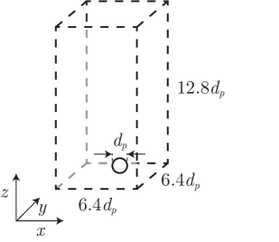
((a)) Layout of a simulation for a rising sphere in a periodic simulation domain. The sphere rises in $z$ direction.

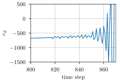
((b)) Oscillations in the drag coefficient $c_{d}$ at $\pi_{p}=0.03$, $\mathrm{Ga}=170$ and $d_{p}=40$.

Figure 2: Test case to study the stability of the coupling approach for a sphere rising inside a box.

To evaluate the approach outlined in Sec. 2 for simulating a light sphere rising in a fluid, we consider the setup shown in Figure 2(a), with a density ratio $\pi_{p}=\rho_{p}/\rho_{f}<1$. The setup comprises a single submerged sphere of diameter $d_{p}$, initially residing at the bottom of the cuboidal domain with dimensions $(6.4,6.4,12.8)d_{p}$. We employ periodic boundary conditions in all directions, and set the initial position of the particle to $(3.2,3.2,0.6)d_{p}$. During the simulation, the particle rises in $z$ direction, as characterized by the Galilei number

$$\mathrm{Ga}=\frac{u_{g}d_{p}}{\nu_{f}},\quad\text{ with }u_{g}=\sqrt{|\pi_{p}-1|gd_{p}}\text{,}$$ (13)

where $g$ is the magnitude of the gravitational acceleration and $u_{g}$ is the characteristic, gravitational velocity. In our simulations, we set $u_{g}=0.01$ in lattice units and use $d_{p}$ to control the overall numerical resolution. Depending on the values for $\pi_{p}$, $\mathrm{Ga}$, and the numerical resolution, the original method can predict the upward motion of the sphere or it may fail by becoming unstable. In the latter case, we observe rapidly growing oscillations of the hydrodynamic force acting on the sphere, as illustrated in Figure 2(b) for an exemplary case. Here, the hydrodynamic force is expressed in terms of the dimensionless drag coefficient ⁵⁷ $c_{d}=2\bm{F}_{p}^{\mathit{hyd}}/\pi_{p}u_{z}\pi r_{p}^{2}$, where $u_{z}$ is the sphere’s vertical velocity and $r_{p}=\nicefrac{{1}}{{2}}d_{p}$. With increasing particle density this behavior is delayed to later stages of the simulation until completely disappearing at a certain density threshold. A simulation is considered stable, if no instabilities occurred until the rising sphere has reached its terminal ascension velocity at normalized time $t_{n}=t/t_{g}=10$, with $t_{g}=d_{p}/u_{g}$.

Table 1: Lowest density ratios $\pi_{p,min}$ at $\mathrm{Ga}=100$ and a certain sphere diameter $d_{p}$ for which stable results can be obtained with MEM-LBM-coupled LBM and particle phases.

$d_{p}/\Delta x$	10	15	20	30	40	50	80
$\pi_{p,min}$	0.13	0.09	0.066	0.045	0.034	0.03	0.02

Table 1 lists the minimum density ratio $\pi_{p,min}$ for which we observe stable results at a certain $d_{p}$ for $\mathrm{Ga}=100$. Most notably, $\pi_{p,min}$ behaves close to inversely proportional to the sphere diameter: For instance, at a diameter of 20, 0.066 is the lowest achievable value of $\pi_{p}$, while at the doubled diameter (40) approximately half the density ratio (0.034) is possible to simulate. The increase in diameter entails a finer resolution of the particle-fluid interface, such that stability issues occur at smaller density ratios. However, every increase in resolution comes with a significant increase in computational costs, such that an alternative approach is required for simulating very light particles efficiently. As such, these observations establish a baseline for possible improvements.

3.2 Analysis of the Instabilities

During each time step of our numerical method, the hydrodynamic interaction forces and torques are first applied to the particle and then a time step for the particle is executed⁴⁶. Thus, these interactions always incorporate a time lag depending on the spatial and temporal resolution. Additionally, also the liquid in the vicinity of a particle must be accelerated together with the particle. This is known as the added mass effect. With an explicit fluid-particle coupling, however, this effect will be accounted for with a time delay. For heavy submerged particles, the added mass effect only plays a minor role and thus does not affect the dynamics. In contrast, for very light particles, the inertial forces originate mainly from the attached fluid mass being accelerated together with the particle ⁴⁵. Hence, even though the inherent inaccuracies are minor, they may lead to oscillations whose amplitude grows.

This issue becomes clear by a closer inspection of the equations that describe the temporal evolution of the linear and angular velocity of a single spherical particle submerged in fluid. In general, these equations for geometrically fully resolving simulations are given as

$$\dfrac{\text{d}\bm{u}_{p}}{\mathop{}\!\mathrm{d}t}=\dfrac{\rho_{f}}{m_{p}}\int_{S}\bm{\tau}\cdot\bm{n}\mathop{}\!\mathrm{d}S+\dfrac{(\rho_{p}-\rho_{f})V_{p}}{m_{p}}\bm{g}=\dfrac{1}{\pi_{p}V_{p}}\int_{S}\bm{\tau}\cdot\bm{n}\mathop{}\!\mathrm{d}S+(\pi_{p}-1)\bm{g}=\dfrac{1}{\pi_{p}V_{p}}(\bm{F}_{p}^{\mathit{hyd}}+\bm{F}_{p}^{\mathit{g}})$$ (14)

and

$$\dfrac{\text{d}\bm{\omega}_{p}}{\mathop{}\!\mathrm{d}t}=\dfrac{\rho_{f}}{I_{p}}\int_{S}\bm{r}\times(\bm{\tau}\cdot\bm{n})\mathop{}\!\mathrm{d}S=\dfrac{1}{\nicefrac{{2}}{{5}}\pi_{p}V_{p}r_{p}^{2}}\int_{S}\bm{r}\times(\bm{\tau}\cdot\bm{n})\mathop{}\!\mathrm{d}S=\dfrac{1}{\nicefrac{{2}}{{5}}\pi_{p}V_{p}r_{p}^{2}}\bm{T}_{p}^{\mathit{hyd}}\text{.}$$ (15)

Here, $\bm{\tau}$ is the hydrodynamic stress tensor, $\bm{n}$ the normal vector of the particle surface $S$, and $\bm{r}$ the vector from the particle center to a point on its surface $S$ ^{45, 38}. For a spherical particle with radius $r_{p}$, $I_{p}$ is given as $\nicefrac{{2}}{{5}}m_{p}r_{p}^{2}$.

For very light particles, i.e. $\pi_{p}\rightarrow 0$, the coupling relations become singular due to a vanishing denominator in Equations 14 and 15. In other cases, a small denominator with $\pi_{p}\ll 1$ results in a large factor magnifying the fluid contribution. This amplifies inaccuracies originating from the numerical computation of $\bm{F}_{p}^{\mathit{hyd}}$ and $\bm{T}_{p}^{\mathit{hyd}}$ in explicit fluid-particle coupling approaches ⁴⁵.

3.3 Virtual Mass Correction for the LBM

This shortcoming for simulations of light particles can be overcome by the virtual mass approach of Schwarz et al. ⁴⁵. This approach has originally been developed for a classical Navier-Stokes-based solver in combination with the immersed boundary method (IBM) ³⁸. The therein applied IBM originally struggled with density ratios lower than $0.4$ due to oscillations in angular and translational velocities leading to a divergence within only few time steps ⁴⁵. This detrimental behavior is therefore similar to the one we observed for the MEM-LBM-coupled simulations.

Here, we aim to employ the same stabilization technique to the LBM with the MEM-based particle coupling, following the arguments provided by Schwarz et al.⁴⁵ for the IBM. Alike the IBM, our numerical method accounts for the same Equations 14 and 15. Following Schwarz et al.⁴⁵, we introduce the concept of a virtual force

$$\bm{F}_{p}^{\mathit{v}}=m_{p}^{v}\tfrac{\mathrm{d}\bm{u}_{p}}{\mathrm{d}t}.$$ (16)

It uses the virtual mass $m_{p}^{v}=C_{v}\rho_{f}V_{p}$, which introduces the virtual mass coefficient $C_{v}>0$. Adding the virtual force $\bm{F}_{p}^{\mathit{v}}$ to both sides of Equation 14 and rearranging yields

$$\dfrac{\text{d}\bm{u}_{p}}{\mathop{}\!\mathrm{d}t}=\dfrac{1}{(C_{v}+\pi_{p})V_{p}}\int_{S}\bm{\tau}\cdot\bm{n}\mathop{}\!\mathrm{d}S+\dfrac{\pi_{p}-1}{C_{v}+\pi_{p}}\bm{g}+\dfrac{C_{v}}{C_{v}+\pi_{p}}\dfrac{\text{d}\bm{u}_{p}}{\mathop{}\!\mathrm{d}t}.$$ (17)

A direct comparison with Equation 17 reveals, that this corresponds to a particle with altered mass $m_{p}+m_{p}^{v}$ onto which an additional force $\bm{F}_{p}^{\mathit{v}}$ is acting that exactly compensates the effect of the increased mass. We explicitly note that this virtual force is different from the added mass force, a physically observable effect which is already accounted for in the geometrically fully-resolved simulation model, as we employ it here. The virtual mass coefficient $C_{v}$ may be determined on an empirical basis. To attain a positive effect, $C_{v}$ has to be large enough depending on the density ratio. For spherical particles, Schwarz et al. propose to use $C_{v}=0.5$ referring to the added mass coefficient of submerged spheres ⁴⁵. In our case, values of 0.5 or 1 were found to be suitable, which also satisfy the condition of a lower limit recently reported by Tavanashad et al. ⁵⁸.

In Equation 17 the derivative of the translational particle velocity appears on either side of the equation. Physically, this is well justified, as the effect induced by the virtual mass should be exactly suppressed by the counteracting force. From an algorithmic perspective, this prevents an explicit temporal integration. As the acceleration in the current time step is to be computed and thus unknown, the acceleration on the right hand side must be approximated to allow explicit integration. Schwarz et al. employ second order Lagrange interpolation using the three most recent velocities in order to extrapolate the acceleration⁴⁵. Here, we alternatively propose to use the particle’s acceleration from the previous time step as computed during the Velocity Verlet procedure (Section 2.2). This essentially simplifies the scheme, reduces memory consumption, and showed the most promising results in our prestudies. Denoting the previous translational acceleration as $\bm{a}_{p,t-1}$ then leads to

$$\dfrac{\text{d}\bm{u}_{p}}{\mathop{}\!\mathrm{d}t}\approx\dfrac{1}{(C_{v}+\pi_{p})V_{p}}\int_{S}\bm{\tau}\cdot\bm{n}\mathop{}\!\mathrm{d}S+\dfrac{\pi_{p}-1}{C_{v}+\pi_{p}}\bm{g}+\dfrac{C_{v}}{C_{v}+\pi_{p}}\bm{a}_{p,t-1}\text{.}$$ (18)

Similarly, the equation for angular motion Equation 15 is complemented with a virtual torque

$$\bm{T}_{p}^{\mathit{v}}=\nicefrac{{2}}{{5}}C_{v,\omega}\rho_{f}V_{p}r_{p}^{2}\tfrac{\mathrm{d}\bm{\omega}_{p}}{\mathrm{d}t},$$ (19)

where the coefficient $C_{v,\omega}$ serves the same purpose as $C_{v}$ for the translational component. Substituting the angular acceleration on the right hand side for an estimate $\bm{\beta}_{p,t-1}$ and rearranging gives

$$\dfrac{\text{d}\bm{\omega}_{p}}{\mathop{}\!\mathrm{d}t}\approx\dfrac{1}{\nicefrac{{2}}{{5}}V_{p}r_{p}^{2}(C_{v,\omega}+\pi_{p})}\int_{S}\bm{r}\times(\bm{\tau}\cdot\bm{n})\mathop{}\!\mathrm{d}S+\dfrac{C_{v,\omega}}{C_{v,\omega}+\pi_{p}}\bm{\beta}_{p,t-1}\text{.}$$ (20)

Consequently, Equations 7a and 7c now contain $\bm{F}_{p}^{\mathit{v}}$ and $\bm{T}_{p}^{\mathit{v}}$, such that $\bm{F}_{p}=\bm{F}_{p}^{\mathit{hyd}}+\bm{F}_{p}^{\mathit{g}}+\bm{F}_{p}^{\mathit{v}}$ and $\bm{T}_{p}=\bm{T}_{p}^{\mathit{hyd}}+\bm{T}_{p}^{\mathit{v}}$. The therein applied mass and moment of inertia are now given by $m_{p}=(\rho_{p}+C_{v}\rho_{f})V_{p}$ and $I_{p}=\nicefrac{{2}}{{5}}(\rho_{p}+C_{v,\omega}\rho_{f})V_{p}r_{p}^{2}$, respectively.

Finally, Algorithm 1 outlines the complete simulation algorithm, featuring the steps introduced by the virtual mass correction in green. The update of the flow field via LBM, and the successive computation of the hydrodynamic interactions remains untouched, as well as the computation of the submerged weight force. Then, the virtual force and torque are computed based on the translational and rotational accelerations of the previous time step. The integrator of the particle is supplied with the virtually increased mass to update the particle’s position and velocities. For the remainder of the paper, we will refer to this approach as VM-MEM-LBM, in contrast to the original MEM-LBM from Section 2 that does not apply the green parts.

Algorithm 1 Outline of VM-MEM-LBM for a single submerged particle.

1:for each simulation step do

2:     Perform LBM step.

3:     Compute hydrodynamic interactions, and average over two time steps.

4:     Set buoyant and gravitational force.

5:     Calculate virtual force and torque.

6:     Update particle’s translational and angular velocity with virtually increased mass.

7:     Update the particle mapping into the fluid domain.

8:end for

3.4 Validation

For validating the translational and angular components of the virtual mass approach, two different scenarios are applied next. For moderate density ratios the unchanged MEM-LBM, Section 2, is used as a reference, together with results from Ref. 45 where similar validation setups were used.

3.4.1 Virtual Added Mass Force

To validate Equation 18, we employ the same setup and parameterization as described in Section 3.1. A first set of simulations are carried out with Galileo number $\mathrm{Ga}=100$ at density ratios $\pi_{p}\in\left\{0.1,1.1\right\}$ and a resolution of $d_{p}=40$, where the MEM-LBM serves as a reference. A final test run at $\pi_{p}=0.001$, which is well below the minimal density ratio for which we expect stable simulations using MEM-LBM and a sphere diameter of 40 cells, employs a Galileo number of $170$ and reference data is extracted from Ref.45. For VM-MEM-LBM, we use $C_{v}=1$ in all cases.

The normalized ascension velocity of the particle is given as $u_{z,n}=u_{z}/u_{g}$. Its mean squared error $\overline{\epsilon}_{sq}$ and mean relative error $\overline{\epsilon}_{rel}$ with respect to a reference $\hat{u}_{z,n}$ evaluated at $m$ points in time are defined as

$$\overline{\epsilon}_{sq} =\tfrac{1}{m}\sum_{i}^{m}\left(u_{z,n,i}-\hat{u}_{z,n,i}\right)^{2}\text{,}$$ (21)

$$\overline{\epsilon}_{rel} =\tfrac{1}{m}\sum_{i}^{m}\dfrac{u_{z,n,i}-\hat{u}_{z,n,i}}{\hat{u}_{z,n,i}}\text{.}$$ (22)

Additionally, the relative error in the terminal velocity is given as $\epsilon_{term,rel}=\left(u_{z,n,term}-\hat{u}_{z,n,term}\right)/\hat{u}_{z,n,term}$.

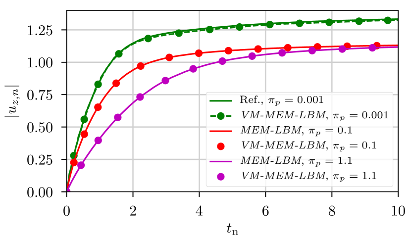
((a)) Complete run.

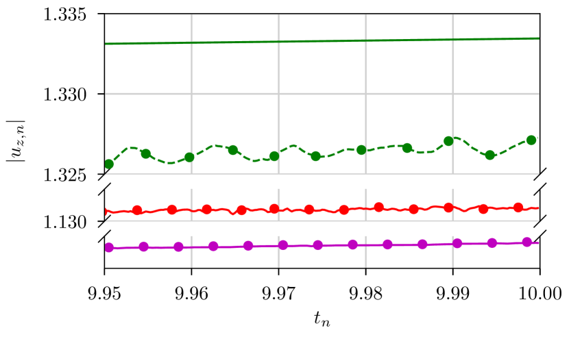
((b)) Magnification of end.

Figure 3: Normalized rising velocities for the validation runs using VM-MEM-LBM compared with their references. In case of $\pi_{p}=0.001$, reference data is extracted from Ref. 45. For density ratios $>0.001$, the MEM-LBM served as base line.

In Figure 3(a), the particle velocities of the simulations employing the VM-MEM-LBM are compared with their reference. Overall, all density ratios show very good agreement during the whole simulation. Yet, $\pi_{p}=0.001$ deviates slightly from the reference after $t_{n}\approx 2$. The magnified view of the terminal velocities in Figure 3(b) shows light particles exhibiting an oscillating behavior with small amplitude of less than 0.1% of $u_{z,n}$. For heavier particles, these oscillations cannot be observed.

Table 2: Resulting particle Reynolds number $\real_{p}=u_{z,term}d_{p}/\nu$ and errors in the normalized translational velocity $|u_{n}|$ when comparing the VM-MEM with reference data. Mean squared error $\overline{\epsilon}_{sq}$ and mean and terminal errors ($\overline{\epsilon}_{rel}$ and $\epsilon_{term,rel}$, respectively) relative to the reference velocities.

$\pi_{p}$	$0.001$	$0.1$	$1.1$
$\mathrm{Ga}$	$170$	$100$	$100$
$\real_{p}$	$225.64$	$113.08$	$111.77$
$\overline{\epsilon}_{sq}$	$0.01\text{\cdot}{10}^{-3}$	$15.48\text{\cdot}{10}^{-9}$	$1.85\text{\cdot}{10}^{-9}$
$\overline{\epsilon}_{rel}$	$0.86\text{\cdot}{10}^{-3}$	$0.28\text{\cdot}{10}^{-3}$	$0.15\text{\cdot}{10}^{-3}$
$\epsilon_{term,rel}$	$4.64\text{\cdot}{10}^{-3}$	$0.04\text{\cdot}{10}^{-3}$	$0.06\text{\cdot}{10}^{-3}$

Visible in Table 2, across all density ratios the VM-MEM-LBM performs very well when compared with reference data. The mean relative errors $\overline{\epsilon}_{rel}$ amount to less than $0.3\cdot 10^{-3}$ for all cases with a density ratio $\pi_{p}\geq 0.1$ (Table 2). However, the mean squared error is much larger in the comparison of the simulation at $\pi_{p}=0.1$. This results from fluctuations in the velocities, observable in Figure 3. In the terminal velocity, the relative error $\epsilon_{term,rel}$ for the three larger density ratios again is almost nonexistent, listed in Table 2. At an increased terminal deviation of $\epsilon_{term,rel}=4.64\cdot 10^{-3}$, the error of the simulation with density ratio $\pi_{p}=0.001$ is still within reasonable bounds.

Schwarz et al. initially report a relative error in the particle velocity of approximately $2\%$ for their general scheme ⁴⁵. After adjusting the forcing point positions of the particle-fluid-coupling in their simulations they achieve a lower error of $2\cdot 10^{-3}$, similar to our results.

3.4.2 Virtual Added Mass Torque

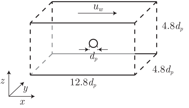
((a)) Domain setup.
                                                                                                                                                 

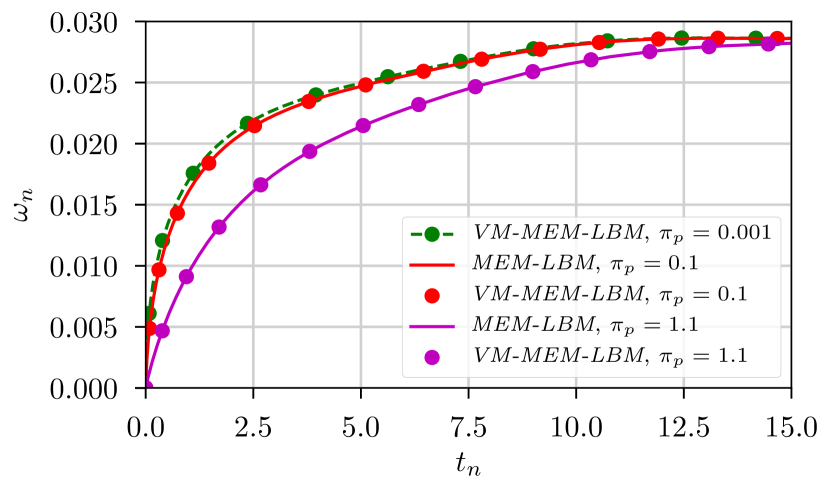
((b)) Normalized angular velocity $\omega_{n}$ for various density ratios, using either MEM-LBM or VM-MEM-LBM.

Figure 4: Test case (4(a)) and error (4(b)) to validate the VM-MEM-LBM with respect to rotation. While the sphere’s position is fixed throughout the simulation, the upper wall moving with velocity $u_{w}$ drives the Couette-initialized fluid, rotating the sphere after free rotation is unblocked.

Similar to Ref. 45, this test case features a domain of size $(12.8,6.4,4.8)d_{p}$, confined by two walls in $z$ direction and periodic otherwise. A sphere of $40$ cells in diameter is positioned in the domain center $(6.4,3.2,2.4)d_{p}$. Here, the sphere is kept fixed at its initial position and all degrees of freedom are blocked at first. The fluid is initialized with a Couette profile, which is further driven by the upper moving wall at a constant velocity $u_{w}=0.1$ in $x$ direction during the simulation. This induces an angular momentum onto the particle, as sketched in Figure 4(a). After the flow field has fully developed, rotation of the particle is allowed and its rotational velocity over time is monitored.

The setup is defined by the density ratio $\pi_{p}$ and the particle Reynolds number $\real_{p}=u_{p}d_{p}/\nu$, where $u_{p}$ is the undisturbed fluid velocity at the sphere’s position. Since the sphere resides in the center of the domain, the fluid velocity evaluates to $u_{p}=\nicefrac{{1}}{{2}}u_{w}$. The Reynolds number $\real_{p}=110$ is chosen to approximately match the situation in the force validation study in Section 3.4.1. For $\pi_{p}\in\left\{0.1,1.1\right\}$, we again compare the results to MEM-LBM. Additionally, $\pi_{p}=0.001$ is tested to check stability of VM-MEM-LBM in contrast to the, for this case, unstable MEM-LBM. We define $t_{c}=d_{p}/u_{p}$ and $\omega_{c}=u_{p}/d_{p}$ to normalize the time scale and the angular velocity, resulting in $t_{n}=t/t_{c}$ and $\omega_{n}=\omega_{y}/\omega_{c}$, respectively.

As displayed in Figure 4(b), simulations that employ the virtual mass correction agree very well to the reference data. The mean relative errors are below $0.5\cdot 10^{-3}$ for both cases, see Table 3. We point out that the terminal angular velocities match almost exactly. The proof-of-concept simulation at density ratio $0.001$ also appears to have performed well, with a plausible trend in angular velocity and, as expected, a stronger angular acceleration than the heavier spheres.

Table 3: Errors in the normalized angular velocity $\omega_{n}$ for VM-MEM-LBM compared to simulations using MEM-LBM.

$\pi_{p}$	$0.1$	$1.1$
$\overline{\epsilon}_{rel}$	$0.46\text{\cdot}{10}^{-3}$	$0.15\text{\cdot}{10}^{-3}$
$\epsilon_{term,rel}$	$0.01\text{\cdot}{10}^{-3}$	$0.0\text{\cdot}{10}^{-3}$

3.5 Discussion

We have demonstrated that the virtual mass corrections can be successfully adapted to the momentum exchange method. Thus, the originally observed oscillations in the motion of very light particles are effectively reduced and stable simulations are obtained. As the VM-MEM-LBM relies on an approximation of the particle’s acceleration, the introduction of a certain error in comparison to MEM-LBM is unavoidable, as also observed in Ref. 45. The validation scenarios reveal that this error is very small: In the rising particle setup of Section 3.4.1 the error stays below $0.5\%$, for the cases with $\pi_{p}\geq 0.1$ well below that. Evaluating the accuracy of angular motion in Section 3.4.2, the error thresholds for density ratios $\pi_{p}\in\{0.1,1.1\}$ are similarly low at $0.05\%$, at most. Nevertheless, even though the virtual mass was introduced as a solely numerically stabilizing technique for explicit fluid-particle coupling schemes, the VM-MEM-LBM might alter the physical results of the simulation. In phases with high acceleration changes, it artificially increases inertia by relying on the past acceleration value. Thus, for those phases, where the virtual force approximation might affect the accuracy negatively, choosing a rather low value of $C_{v}$ is advisable. In all our cases, values of $0.5$ or $1$ were found to be sufficient. These arguments will be revisited in Section 5, where the VM-MEM-LBM again serves to simulate a sphere at $\pi_{p}=0.001$ and results are compared to literature.

In a recent work, Tavanashad et al. ⁵⁸ discussed the constant $C_{v}$ more extensively and established a lower positive limit for $C_{v}$, depending on the density ratio and the added mass coefficient. Our choice of $C_{v}$ is in line with this limit.

4 Adaptive Grid Refinement

Accurate numerical studies of particle rising in a fluid, as they will be carried out in Section 5, require large computational domains to reduce the influence of the boundary conditions on the trajectories. On the other hand, ensuring an adequate representation of boundary layers along the particle’s surface and of the vortex structures necessitates a fine numerical resolution in those regions. Using a uniform grid for such simulations would result in enormous computational costs and limit the parameter space that can be explored substantially. To alleviate this problem, we apply adaptive grid refinement in this work which significantly reduces the required computational resources. In this section, we briefly outline and validate the grid refinement technique. The method makes use of the domain partitioning functionalities provided by the waLBerla framework ^{59, 32}.

4.1 Block-structured Grid Refinement with LBM

Using a block-structured domain partitioning, the computational domain is split into so-called blocks, each containing a lattice of uniformly sized cells ³². Grid refinement is then carried out by uniformly dividing a block into eight smaller blocks, if needed. A block on the coarsest refinement level then has level $l=0$, while blocks on the finest level have level $l=l_{max}$. As each block features the same number of cells, the grid spacing $\Delta x_{l}$ of a block gets smaller with increasing level according to $\Delta x_{l+1}=\nicefrac{{1}}{{2}}\Delta x_{l}$. Overall, a 2:1 balance between the blocks is maintained, meaning that the refinement level of neighboring blocks must at most differ by one.

A lattice Boltzmann method, capable of dealing with such non-uniform grids, was proposed by Rhode et al. ⁶⁰ and is applied here. Details about its efficient implementation can be found in Refs. 59, 61.

4.2 Refinement Criteria

The refinement structure is defined by the individual target level of each block. Criteria determining the target level are presented below. They are checked regularly throughout the simulation and their result is combined to satisfy all constistency requirements. Subsequently, if some blocks are found to be on an unsuitable level of refinement, the grid is adapted by either coarsening or refining the blocks, obeying the 2:1 restriction.

4.2.1 Particle-based Refinement Criteria

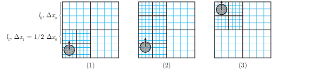
Figure 5: Refinement depending on the presence of a particle. Blocks are outlined black, containing 4x4 cells (outlined blue). (1) In the beginning, the block hosting the particle and its direct neighbors are on the finest level. (2) As soon as the particle enters the next block in vertical direction, the upper left non-refined block notices its presence in one of its lower neighbors and refines. (3) The particle now is fully contained within the upper quarter of the domain, such that the formerly four fine blocks at the bottom all are available to coarsen to one block. The frequency of the refinement evaluations has to be high enough to catch those particle movements, such that it always resides on the finest grid.

During the simulation, we ensure that blocks that are in the vicinity of particles are always on the finest grid. This is motivated by both algorithmic and physical reasons. From an algorithmic perspective, we avoid the software complexity of maintaining a consistent particle mapping across different refinement levels. At the same time, this refinement rule ensures that the finest resolution is used to resolve the boundary layer around the particle. In these regions high velocity gradients occur and are thus resolved with maximal resolution.

Alternatively, in a block where no particle is nearby, the refinement level would be allowed to become coarser. Here other refinement criteria apply combined with the 2:1 balance between neighboring blocks. A typical scenario is illustrated in Figure 5.

4.2.2 Flow Structure-based Refinement Criteria

Secondly, special algorithmic sensors are applied to the fluid to compute criteria for the refinement of a block. In our case, $\phi_{c}$, the scaled curl of the velocity field, is evaluated to detect shear layers and to control the resolution of high velocity gradients ^{62, 63, 64}:

$$\phi_{c}=|\nabla\times\bm{u}_{f}|s^{(r+1)/r}\text{.}$$ (23)

Here, $\bm{u}_{f}$ denotes the cell local fluid velocity, $s$ a characteristic length scale for a cell and $r$ a weighting coefficient. Multiplying by the weighted length scale $s^{(r+1)/r}$ facilitates the detection of weaker features in a coarser grid area, allowing weaker features to be refined when the stronger ones have been resolved ⁶⁵. The length scale $s$ can be chosen as $\sqrt[3]{V_{cell}}$ with $V_{cell}$ as the volume of a cell or, for cubical cells, simply $\Delta x$. The constant $r$ is commonly assigned a value of $2$ ^{62, 63, 64}. A user-defined threshold $\sigma_{c}$ enables the adaptive manner of the fluid phase. Refinement is triggered when $\phi_{c}>\sigma_{c}$, while coarsening when $\phi_{c}<c\sigma_{c}$. To avoid repetitive refinement and coarsening, the value of $c$ should be lower than $1/2^{(r+1)/r}$, i.e. $c\lesssim 0.35$ for $r=2$ ⁶³.

4.3 Validation

To evaluate the accuracy and performance, we compare adaptive grid refinement against a simulation using a uniform grid. The parameters are chosen to reflect a typical setup as used in the next section. In particular, we use the Galileo number $\mathrm{Ga}=300$ and a density ratio of $0.5$ for a sphere of diameter $d_{p}=100$. These properties do not require the application of VM-MEM-LBM to stably couple solid and fluid phases, such that the MEM-LBM is employed. The domain is fully periodic and of size (7.68, 7.68, 53.76)$d_{p}$. The sphere is positioned initially at (3.84, 3.84, 0.6)$d_{p}$. Starting from this point, the sphere rises up to and reaches $z_{n}=z/d_{p}=50$ at time $t_{n}=36$. In that time span we can observe the beginning of a zig-zagging motion as depicted in Figure 7. Based on this scenario, we validate the sphere’s trajectory in an adaptively refining grid against the one in a fully resolved reference simulation.

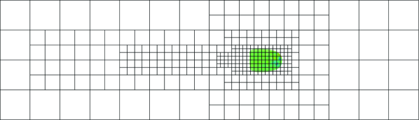
((a)) Adaptively refined grid.

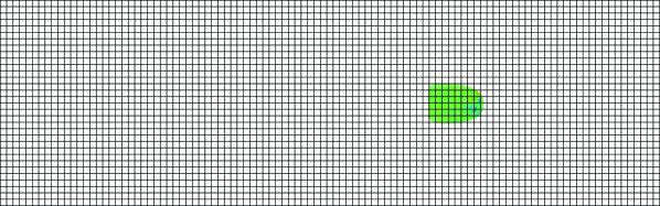
((b)) Uniform grid.

Figure 6: Domain partitioning at $t_{n}\approx 12.5$ in the adaptive and uniform case. The black lines depict the outline of the blocks. Only the lower region of the simulation domain is shown, where the primary movement direction ($z$) of the sphere is from left to right. The vortices around the particle are visualized using the Q criterion ⁶⁶.

In the adaptively refined scenario, we set the refinement threshold $\sigma_{c}$ to $0.001$ and the coarsening factor $c$ to $0.2$. According to those values, a block is assigned one of 6 possible levels of refinement. A visual comparison of the resulting domain partitioning for a small part of the domain is provided in Figure 6(a), which shows the outline of the blocks, each containing $24^{3}$ cells. The flow field around the rising sphere is visualized by the Q criterion ⁶⁶ for a time step right before the zig-zagging motion begins.

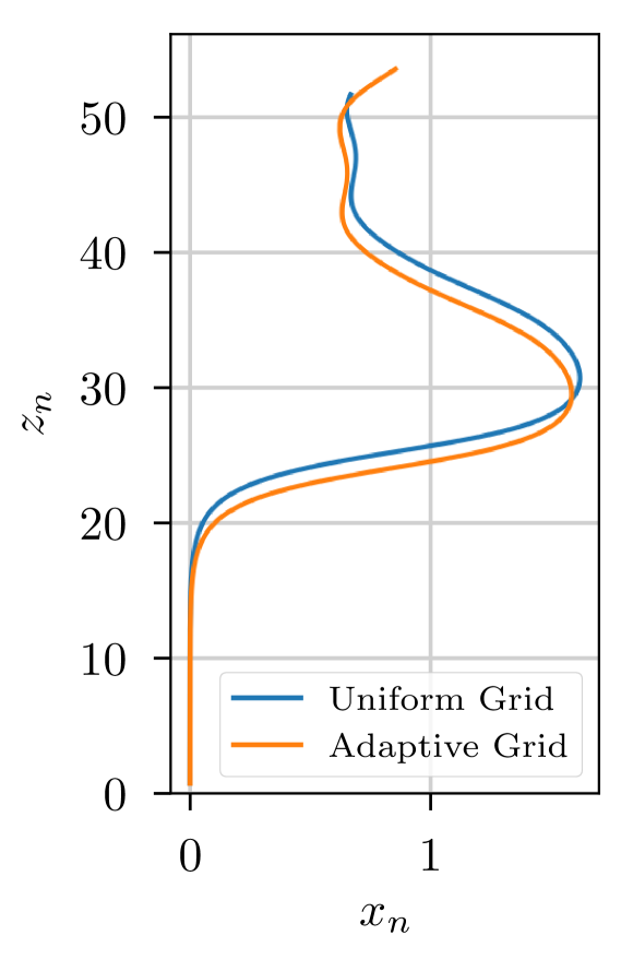
((a)) Particle displacement.

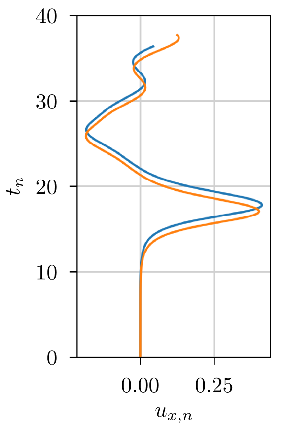
((b)) Velocity.

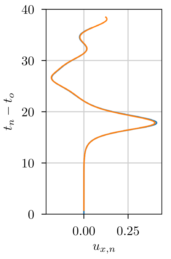
((c)) Aligned velocities.

Figure 7: Comparison of particle trajectory and velocity for adaptively refined (orange) and uniform (blue) simulation at $\mathrm{Ga}=300$ and $\pi_{p}=0.5$. Coordinates are normalized by particle diameter $d_{p}$, velocities by $u_{g}$.

As the results show in Figure 7, the adaptively refined simulation behaves in the same manner as the one using a uniform grid after the initial trigger of the horizontal motion appears at a slight delay. The particle trajectory resides in a vertical plane, which is rotated by $45\degree$ in the horizontal plane. Figure 7(a) shows the normalized vertical over the horizontal sphere displacement.

By defining a time $t_{o}$ at which the horizontal sphere velocity deviates from 0 and thus marks the beginning of the path-instability, we obtain a delay of $\Delta t_{n}=t_{o}^{uniform}-t_{o}^{refined}\approx 0.75$. This observed delay is attributed to the unpredictable and to a certain degree random appearance of the path-instability. By accounting for this delay while plotting the velocity in Figure 7(c), the two lines essentially collapse into a single one. A mean relative error between the aligned velocities of $1.1\%$ further underlines the agreement between both simulations and shows that the adaptive resolution introduces no substantial error in predicting the zig-zagging trajectory of the particle.

Table 4: Comparison of setup and computational costs of the uniform and grid refinement scenario.

Grid	(avg.) #cells	(avg.) #blocks	#processes	run time (hours)	total core hours
Uniform	$3.06\cdot 10^{9}$	$221184$	$36864$	$10.27$	$378474$
Adaptive	$3.78\cdot 10^{7}$	$2738.74$	$768$	$6.58$	$5337$

Regarding the computational resources of both simulations, the respective setup is described in Tab. 4 and was run on the SuperMUC-NG supercomputer at LRZ in Garching. Besides the reduction of the number of cells, the LBM for non-uniform grids carries out less time steps on coarser grids ⁶⁰ which further increases the efficiency of the grid refinement approach. We find that the adaptively refined grid scenario reduced the required total core hours by a factor of 71. In our case, we thus could obtain the essentially same results in less time and using significantly less processes.

As such, we have demonstrated that the here proposed grid refinement approach is capable of drastically reducing the computational costs of such a simulation while maintaining the accuracy of the uniform grid. In combination with the virtual mass correction, this enables efficient simulations of rising particles with very small density ratios.

5 Numerical study of rising particles

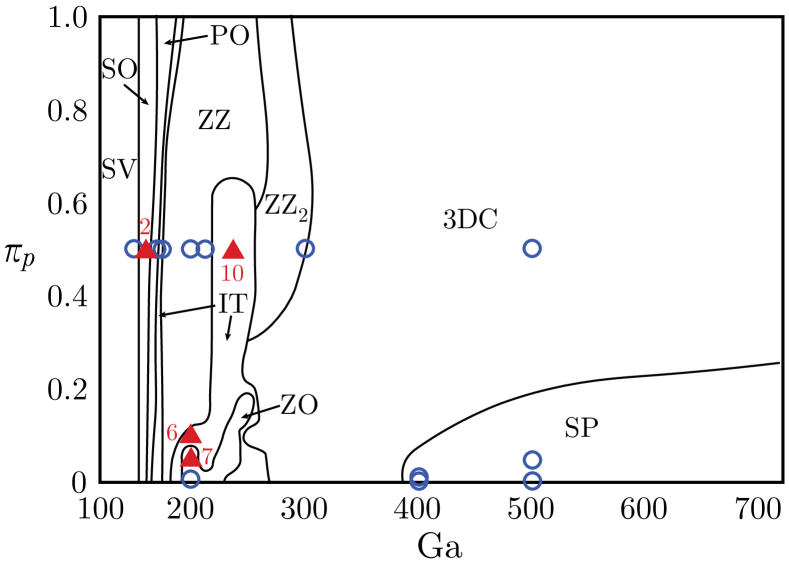
	Description
SV	Steady vertical
SO	Steady oblique
PO	Periodic oblique
ZZ	Zig-zagging
ZO	Oblique zig-zagging
IT	Intermittent
3DC	Three-dimensionally chaotic
SP	Spiraling

Figure 8: Regimes of particle motion characterized by density ratio $\pi_{p}$ and Galilei number $\mathrm{Ga}$ according to Ref. 20. Overlaid points correspond to our simulations. Numbered triangles mark simulations at least partly differing from Auguste & Magnaudet’s results, circles largely confirm those.

The trajectories of light ascending particles have attracted growing interest since they may exhibit different regimes depending on certain parameters ¹⁷. With increasing computational power, also numerical simulations became possible ^{67, 15, 16, 19, 20}. In their work from 2004, Jenny, Dušek & Bouchet ¹⁵ showed that the type of trajectory is mainly determined by two parameters, the density ratio $\pi_{p}$ and the Galilei number $\mathrm{Ga}$, which describes the ratio of buoyant and viscous effects. They used numerical simulation to examine the particle paths that are encountered when varying $\pi_{p}\in[0,10]$ and $\mathrm{Ga}\in[150,350]$. In their work, they solve the Navier-Stokes equation based on a spectral-element spatial discretization in a cylindrical domain moving with the sphere. In particular, Jenny et al. isolated several regions in the parameter space, where rising spheres would show complex movements. The possible regimes range from steady vertical to three-dimensional chaotic, with an oblique and oblique zig-zagging regime in between.

Horowitz & Williamson ¹⁷ performed a comprehensive experimental study across a wide range of sphere densities and Reynolds numbers. Most notably, they identified a “critical mass” ratio, which marked the transition between a steady rise (for a sphere with a density ratio bigger than the critical value) and zig-zagging for a certain Reynolds number beyond the one corresponding to the loss of axisymmetry in the wake. The critical mass ratio amounted to $0.36\pm 0.03$ for $\real\in[260,1550]$ and to $0.61$ for Reynolds numbers higher than $1550$.

More recently, Auguste & Magnaudet carried out an extensive set of simulations using a spectral element method on a moving grid²⁰ leading to results illustrated here in Figure 8. Plotting the density ratio against the Galilei number, various patterns of motion emerge with increasing $\mathrm{Ga}$ and varying $\pi_{p}$. Initially they encounter a steady vertical (SV) regime. With further increasing Galilei numbers, steady oblique (SO) and periodic oblique (PO) motion follow. Planar zig-zagging (ZZ) arises next, where during each change of direction and between two crests vortices are shed. Depending on the density ratio, this regime reportedly persists up to $\mathrm{Ga}\approx 250$ for $\pi_{p}\gtrsim 0.6$ and only up to $\mathrm{Ga}\approx 220$ for $0.15\lesssim\pi_{p}\lesssim 0.6$. Small amplitude zig-zags for spheres with density ratio of $\gtrsim 0.6$ in a three dimensional regime termed ZZ₂ follow next; at lower density ratios an intermittent regime (IT) up to $\mathrm{Ga}\approx 250$ occurs first. In a small stride of the map, very light spheres perform oblique zig-zagging (ZO). After a threshold value of $\mathrm{Ga}\approx 250$ to $300$, three dimensional chaotic (3DC) paths are assumed by submerged spheres of all density ratios. Beyond $\mathrm{Ga}\approx 400$ however, some regularity is regained in the spiraling motion (SP) for very light spheres.

Except for some differences at $\mathrm{Ga}=200$ to $250$, these findings agree largely with the ones from Zhou & Dušek ¹⁹, who used a similar numerical method. On the other hand, these numerical results show deviations from the experimental studies of Horowitz & Williamson, who e.g. do not record sphere trajectories pertaining to the 3DC regime.

In the present work, we study 16 combinations of $\mathrm{Ga}$ and $\pi_{p}$ that we simulate with the new method as proposed in this article, if required. This allows us to further validate our method on the one hand, and to investigate the parameter spaces where existing studies report mismatching results. The analyzed parameter combinations are marked in Figure 8.

5.1 Simulation Setup

All simulations are performed in a cuboidal simulation domain with periodic boundary conditions in all directions. Large enough domains are chosen to avoid that turbulent structures spread so far that they would influence the particle wake or the trajectory by re-entering on the opposite side of the domain. Depending on the combination of $\mathrm{Ga}$ and $\pi_{p}$, the sphere is resolved using a varying number of cells per diameter, expressed by $d_{p}/\Delta x$, to assure a fine enough resolution of the boundary layer along the sphere surface and the wake ³⁵. We adjust the parameter $\Lambda_{b}$ of the MRT collision operator as introduced in Section 2.1 to $\Lambda_{b}=1$, which recovers the TRT collision operator.

Table 5: Domain properties and sphere resolution $d_{p}/\Delta x$ used for the simulations of this chapter. Refinement check frequency is expressed in terms of time steps on the coarsest grid level.

Setup	Domain Size	$d_{p}/\Delta x$	Refinement Levels	Refinement Check Freq.
I	(38.4, 38.4, 192)	80	8	4
Il	(38.4, 38.4, 384)	80	8	4
II	(30.72, 30.72, 215.04)	100	8	4
III	(38.4, 38.4, 307.2)	160	9	8

In all cases, adaptive grid refinement, as described in Section 4, is applied to reduce the computational cost. Depending on the domain size, 8 or 9 levels of refinement are applied. The necessity for an adaption of the grid is evaluated every 4 to 8 time steps on the coarsest grid level,. The flow-based refinement criterion from Section 4.2.2 uses $\sigma_{c}=0.001$ and $c=0.2$. Similar to the simulations described in Section 3, the gravitational velocity $u_{g}=0.01$ in lattice units is used which then determines the gravitational acceleration and the kinematic viscosity for the simulation. A summary of the domain size, $d_{p}$ and refinement levels for each of the setups is presented in Table 5. The virtual mass approach from Section 3 in the fluid-solid coupling is only employed when it is required for stable simulations. In the present cases, this is in settings where the particle density $\pi_{p}=0.001$. Then, the virtual mass coefficients are chosen as $C_{v}=C_{v,\omega}=0.5$.

5.2 Simulation Results

The 16 simulations range over of Galilei numbers from $150$ to $500$ at particle densities of $0.5$, $0.1$, $0.05$, $0.01$ and $0.001$. The results for the key indicators are concisely summarized in Table 6. The parameters are selected such that the range of regimes from the existing literature is covered. In particular, we follow Auguste & Magnaudet’s extensive study and perform a subset of their simulations, plus two additional cases (Case 13 and 16 in Table 6).

Cases 1, 3 and 4 match with the descriptions by Auguste & Magnaudet well, pertaining to the simpler patterns of steady vertical or oblique movement. However, a disagreement is found for Case 2 where the Galilei number is specifically chosen to be located in the transition regime between SV and SO. Auguste & Magnaudet identify the SO regime here, while in our simulation the sphere appears to move SV, with visible transitions to an oblique motion.

In the next four cases, 5 to 8, we fix the Galilei number at 200, merely varying the density ratio. Here we observe three different regimes: ZZ, 3DC, and PO. While we find agreement with Auguste & Magnaudet for Cases 5 and 8, simulations 6 and 7 do not produce the PO trajectories as reported by Auguste & Magnaudet. Instead, we observe a chaotic motion of the sphere, only in Case 6 initially resembling a PO path. However, Zhou & Dušek also categorize those into the 3DC regime.

Further increasing the Galilei number and setting the density ratio to $0.5$ in Cases 9 to 11 shows agreement with Auguste & Magnaudet. In addition to the already established ZZ regime in Cases 9 and 10, a second zig-zagging motion, ZZ₂, is identified in Case 11. This is characterized by a higher frequency and a smaller amplitude.

The final five scenarios feature the largest Galilei numbers. They all exhibit a spiraling motion, except Case 14. There, the trajectory loses all regularity resulting in three-dimensional chaotic motion. These findings are again in agreement with Auguste & Magnaudet. Additionally, Zhou & Dušek confirms our results in Cases 13 and 16, since our results for very light spheres (density ratio of $0.001$) match their results for massless spheres.

All in all, we identify similar issues as both previous numerical studies in replicating the experiments of Horowitz & Williamson. A “critical mass ratio” and zig-zagging motion instead of three dimensional chaotic motion at increasing Reynolds numbers could not be found.

Table 6: Results for simulations of a rising sphere at various combinations of Galilei number $\mathrm{Ga}$ and particle density ratio $\pi_{p}$. For comparison, regimes as found by Auguste & Magnaudet (AM) and Zhou & Dušek (ZD) are provided next to ours. Abbreviations are explained in Figure 8. Columns labeled $u_{z,t}$, $t_{n,t}$ and $z_{n,t}$ list the normalized terminal values of the respective quantity. $d_{cr.}$ and $h_{cr.}$ describe the lateral distance and height from one crest to the following crest after completing one iteration of either a spiraling or a zig-zagging path. Regimes from literature are mostly backed by simulations in the respective case; instances, where only a visual classification by diagram is available, are marked with (*).

Case	Setup	Ga	$\pi_{p}$	Regime			Re	Incl. [$\degree$]	St	$d_{cr.}$	$h_{cr.}$	$u_{z,t}$	$z_{n,t}$	$t_{n,t}$
				Present	AM	ZD
1	I	150	0.5	SV	SV	SV	196.2					1.309	191.8	147.9
2	I	162.5	0.5	SV	SO	SO	218.2					1.343	191.8	143.1
3	I	172	0.5	PO	PO	SO	232.0	4.62	0.043			1.348	191.8	144.3
4	Il	175	0.5	PO	ZZ,PO	PO	237.0	4.74	0.042			1.350	354.5	262.6
5	II	200	0.5	ZZ	ZZ	ZZ	277.8		0.018	1.46		1.408	214.8	155.2
6	II	200	0.1	3DC	PO	3DC*	277.5					1.356	214.8	155.1
7	II	200	0.05	PO, 3DC	PO	3DC*	277.9	2.90				1.398	214.8	155.3
8	II	200	0.001	PO	PO	3DC	276.9	3.07	0.045			1.405	214.8	155.6
9	II	212.5	0.5	ZZ	ZZ	3DC	299.1		0.028	1.14		1.421	241.5	172.6
10	II	237.5	0.5	IT, ZZ	ZZ	3DC	344.5	1.34	0.098	0.22		1.449	254.9	177.9
11	II	300	0.5	ZZ2	ZZ2	3DC	447.9		0.099	0.28		1.495	238.3	162.1
12	III	400	0.01	SP	SP	3DC/SP*	591.0		0.070	0.98	14.20	1.475	171.9	117.3
13	III	400	0.001	SP	SP*	SP	586.6		0.070	1.02	14.06	1.466	294.9	201.0
14	III	500	0.5	3DC	3DC	3DC	815.2					1.600	167.2	105.0
15	III	500	0.05	SP	SP	3DC/SP*	757.3		0.067	1.08	13.81	1.510	266.3	177.6
16	III	500	0.001	SP	SP*	SP	729.3	0.20	0.074	1.09	13.22	1.455	264.8	181.0

5.3 Detailed Analysis of Results

In the following subsections, we describe our simulation results in more detail, following the analysis provided by Zhou & Dušek and Auguste & Magnaudet. This enables an in-depth comparison with these studies, based on various quantities of interest that are also provided in Table 6.

In the following, all reported particle displacements are normalized in terms of the sphere diameter $d_{p}$. As such, normalized coordinate axes corresponding to the particle’s trajectory are denoted as $x_{n}$, $y_{n}$ and $z_{n}$. To quantify periodic paths, a dominant frequency $f$ can be defined and expressed as the dimensionless Strouhal number $\mathrm{St}=fd_{p}/u_{z,t}$, see Ref. 20. Here, the quasi-steady vertical velocity $u_{z,t}$ during the rise of the particle serves as reference velocity, normalized beforehand using the gravitational velocity $u_{g}$. The frequency of sphere oscillations is computed by a Fast Fourier transformation of the horizontal component of the velocity and extracting the frequency with the highest amplitude. For comparison with Zhou & Dušek, we compute the normalized frequency as $f_{n}=ft_{g}$. Further, the lateral displacement $d_{cr.}$ and height $h_{cr.}$ are determined from one typical “zig-zag” or one circle of the spiral. Inclination angles with respect to the vertical axis are computed by fitting a straight line by means of linear regression, starting at the beginning of the oblique displacement.

5.3.1 Galilei Numbers $\mathrm{Ga}\leq 175$: Steady Vertical and Oblique

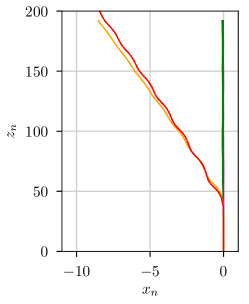
((a)) Steady vertical and oblique ascent.

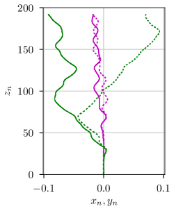
((b)) Minor lateral movement for Cases 1 and 2 ($\mathrm{Ga}=150$ and $162.5$).

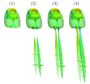
((c)) Wake structure for Case 3. At borders of differently refined regions visualization artifacts formed.

Figure 9: Cases 1 to 4: Plots (a, b) show trajectories at $\pi_{p}=0.5$: $\mathrm{Ga}=150$ (magenta), $162.5$ (green), $172$ (orange) and $175$ (red). Solid lines correspond to movement in $x$ direction, dashed in $y$ direction. In (c) the wake structure of Case 3 is visualized using the Q criterion at a threshold of $10^{-10}$ and colored by normalized vorticity (between $-3.3$, blue, 0 in green and $3.8$, red).

Cases 1 to 4 of Table 6 feature Setup I, covering Galilei numbers from 150 to 175 at a density ratio of $0.5$. We observe steady vertical and oblique movement for these simulations.

At Galilei number 150 (Case 1), the sphere rises in a steady vertical line, with only very minor lateral displacement. This is in line with findings of both Auguste & Magnaudet and Zhou & Dušek.

Case 2 at $\mathrm{Ga}=162.5$ still shows movement corresponding to the SV regime. Yet for Auguste & Magnaudet, this case marked the transition to a second regime with steady oblique movement. A closer inspection of our obtained trajectory hints at a transition to obliqueness (Figure 9(b)), which supposedly is triggered at a slightly higher Galilei number. Unlike Case 1, the path is less oscillating around a vertical axis, but shows especially for the $y$ direction obliqueness with lateral displacement in the order of one tenth of the sphere diameter.

Oblique paths are first observed for Case 3 at $\mathrm{Ga}=172$. This is the first occurrence of a PO path, and corresponds well with Auguste & Magnaudet. Further considering the inclination angle between the trajectory and the vertical axis, Auguste & Magnaudet reported an average value of approximately $4.5\degree$, in comparison to $4.6\degree$ in our case. The comparison Strouhal number $\mathrm{St}=0.05$ is close to the one at hand ($0.043$). Figure 9(c) depicts the wake behind the rising particle: The sphere is constantly enclosed by a flow that builds up and sheds two axisymmetric fluid tubes in regular intervals.

The last case, 4, uses the enlarged Setup I_l to capture a longer impression of the trajectory. The general motion stays the same compared to Case 3, with the inclination slightly changing to $4.74\degree$. Auguste & Magnaudethere noticed zig-zagging at first, which, however, ends after some iterations and changes to an oblique movement, like observed here right from the beginning.

5.3.2 Galilei Numbers $200\leq\mathrm{Ga}\leq 300$: (Oblique) Zig-Zagging and Three Dimensionally Chaotic

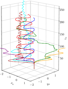
((a)) 3D plot of trajectories at $200\leq\mathrm{Ga}\leq 300$.

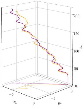
((b)) $\mathrm{Ga}=200$, $\pi_{p}=0.001$ (purple) and $\pi_{p}=0.05$ (orange, mirrored at $(0,0)$).

Figure 10: Cases 5 to 11: Trajectories for the range of Galilei numbers between 200 and 300. Combinations of Galilei number and density ratio depicted as follows. $\mathrm{Ga}=200$: $\pi_{p}=0.5$ (blue), $\pi_{p}=0.1$ (green), $\pi_{p}=0.05$ (orange), $\pi_{p}=0.001$ (purple); $\mathrm{Ga}=212.5$: $\pi_{p}=0.5$ (red); $\mathrm{Ga}=237.5$: $\pi_{p}=0.5$ (cyan); $\mathrm{Ga}=300$: $\pi_{p}=0.5$ (brown).

A series of six simulations (Cases 5 to 11) using Setup II features Galilei numbers between 200 and 300 at various density ratios, as low as $\pi_{p}=0.001$. Following these parametric alterations, vertical and oblique zig-zagging and three dimensionally chaotic regimes emerge.

Various trajectory types are observed at a Galilei number of 200 and three different density ratios. Planar and regular zig-zagging occurs for Case 5 at $\pi_{p}=0.5$, as can be seen in Figures 10(a) and 11(a), where the lateral displacement during each ZZ iteration measures about 1.5$d_{p}$. The Strouhal number is $\mathrm{St}=0.025$. Auguste & Magnaudet did not state detailed numbers for this set of parameters, yet depicted the corresponding path, which matches with ours in Figure 10(a) (blue). Zhou & Dušek more extensively reported on this case, providing a frequency spectrum of the horizontal velocity. They noticed a main peak at $f_{n}=0.035$, which coincides with ours very well ($0.035$). The same can be stated about a second, smaller peak at $f_{n}=0.10$. Furthermore, the descriptions of the particle motion correspond well.

Case 6 lowers the density ratio to $0.1$, yielding an irregular zig-zagging pattern with some obliqueness up to $z_{n}\approx 100$ (Figure 10(a)). Also, three-dimensional motion up to a certain degree is observed. As such, no Strouhal number can be determined. This differs from Auguste & Magnaudet, who report periodic oblique paths here. Only the initial phase up to $z_{n}\approx 70$ agrees qualitatively with their simulations.

Similar observations are made for Case 7 at $\pi_{p}=0.05$ in Figure 10(b), which starts with a regular PO movement, continues obliquely with reduced periodicity and ends chaotic after rising up to $z_{n}\approx 160$. Up until that point, the average inclination of $2.9\degree$ falls within the range of $<3\degree$ reported by Auguste & Magnaudet.

In Case 8, a density ratio of $\pi_{p}=0.001$ is simulated by utilizing the VM-MEM-LBM. Initially, the path resembles the one of the previous Case 7, but stays approximately planar. Additionally, its average inclination of $3\degree$ does not change much during its periodic zig-zags, such that this case can be assigned to the PO regime. As such, a Strouhal number of $0.045$ for the dominant frequency ($f_{n}=0.063$) can be determined. Worth mentioning is the emergence of a second not as pronounced frequency at $f_{n}=0.111$ with $\mathrm{St}=0.079$. While Zhou & Dušek did not provide detailed results on the last three cases, their provided classification suggests chaotic movement for $\mathrm{Ga}=200$ and $\pi_{p}\leq 0.2$.

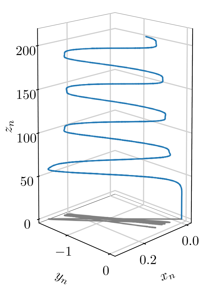
((a)) Case 5: $\mathrm{Ga}=200,\pi_{p}=0.5$: ZZ.

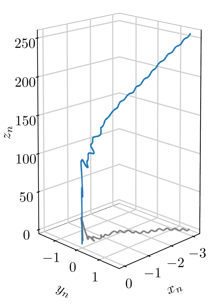
((b)) Case 10: $\mathrm{Ga}=237.5,\pi_{p}=0.5$: ZZ and ZZ₂.

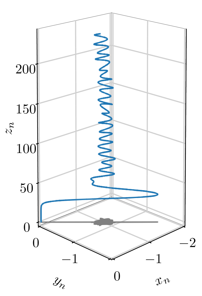
((c)) Case 11: $\mathrm{Ga}=300,\pi_{p}=0.5$: ZZ₂.

Figure 11: Cases 5, 10 and 11: Various cases of zig-zagging in their vertical and horizontal (projected to xy plane) movement.

Case 9 is displayed in Figure 12, where the sphere’s motion at Galilei number of $212.5$ and density ratio of $0.5$ behaves comparable to Case 5. It corresponds to the ZZ regime, slightly tilting its original zig-zagging plane beyond $z_{n}\approx 180$. The projected horizontal displacement of the zig-zagging of approximately $1.5d_{p}$ is also similar. Auguste & Magnaudet identified a Strouhal number ranging from $0.016$ to $0.036$, confirming ours at $\mathrm{St}\approx 0.028$.

Figure 11(b) illustrates the trajectory of a particle at $\mathrm{Ga}=237.5$ and $\pi_{p}=0.5$, corresponding to Case 10. The path starts as ZZ until $z_{n}$ reaches 100 with a Strouhal number of $\mathrm{St}=0.03$, having a large amplitude. Afterwards it enters a slightly inclined plane ($1.37\degree$) with the periodic frequency increasing strongly, leading to $\mathrm{St}\approx 0.10$. This is different from the findings of Auguste & Magnaudet, displaying a movement more prevalent for them at higher Galilei numbers between 250 and 300. At this point, the sphere possibly already enters their ZZ₂ regime, causing a much larger Strouhal number. When considering the simulation at $\mathrm{Ga}=240$ and $\pi_{p}=0.5$ by Zhou & Dušek as reference, their results match with ours with the exception of initial large-amplitude zigzagging, as described.

ZZ₂ is also the regime in which Case 11 with a Galilei number of 300 and density ratio of 0.5 is placed. Its spatial progression is depicted in Figure 11(c). Different from Auguste & Magnaudet’s simulation, we observe an initial lateral swing of magnitude $2d_{p}$, before a more regular oscillatory path is taken. Furthermore, their Strouhal number approximately coincides with ours, at $\mathrm{St}=0.10$. The distance from crest-to-crest is $0.3d_{p}$, as in Auguste & Magnaudet. More so, their observation of a rotating zig-zag plane can be confirmed (see $xy$ plot in Figure 11(c)). The findings of Zhou & Dušek also agree with ours.

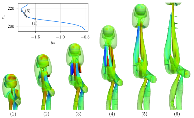
Figure 12: Case 9: Vortices behind a sphere of density ratio $0.5$ at $\mathrm{Ga}=212.5$. Depicted are the states before and during movement through a crest of zig-zagging. A Q criterion threshold of $10^{-10}$ is employed and coloring is done by normalized vorticity, which ranges between -4 (blue) and 4 (red), green corresponding to 0.

5.3.3 Galilei Numbers $\mathrm{Ga}\geq 400$: Spiralling and Three Dimensionally Chaotic

The last simulations cover Galilei numbers of 400 and 500, corresponding to Cases 12 to 16. Depending on the density ratio, we encounter either chaotic movement or a highly regular spiraling regime.

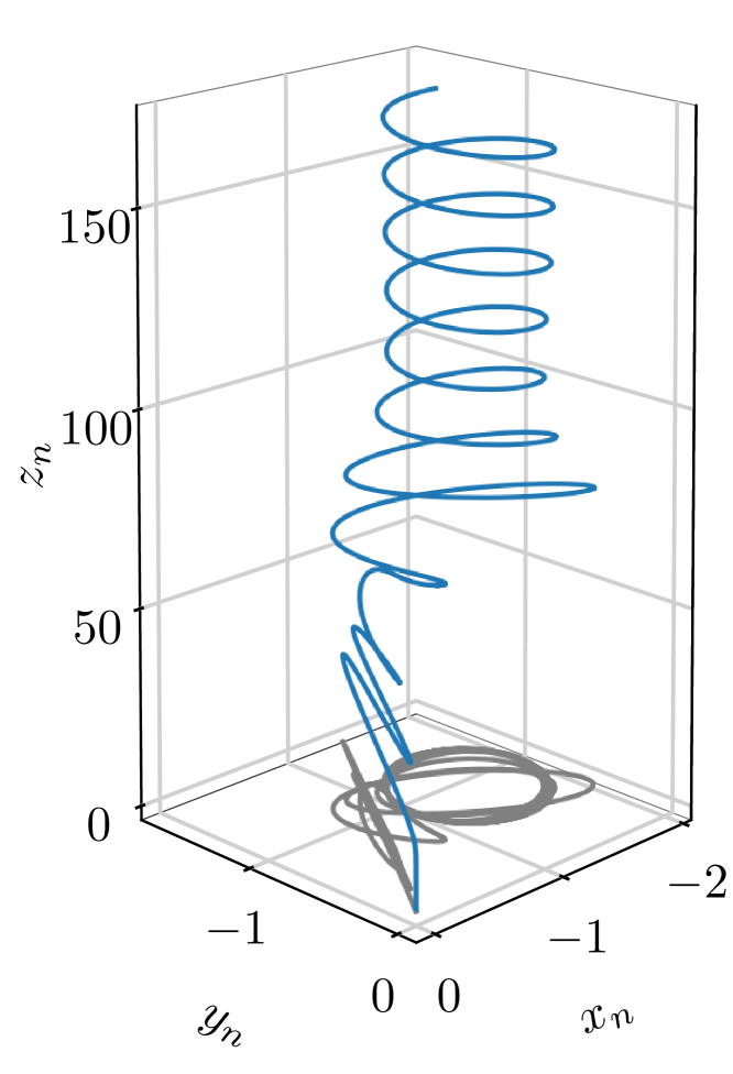
((a)) Case 12: $\mathrm{Ga}=400,\pi_{p}=0.01$: SP.

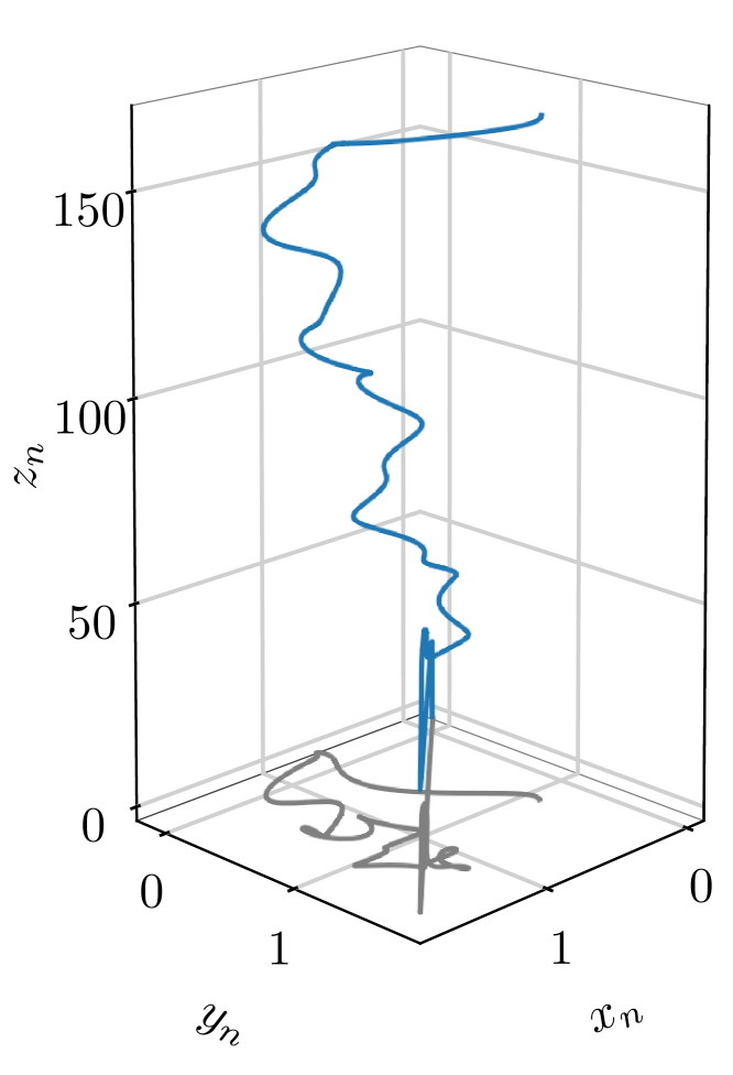
((b)) Case 14: $\mathrm{Ga}=500,\pi_{p}=0.5$: 3DC.

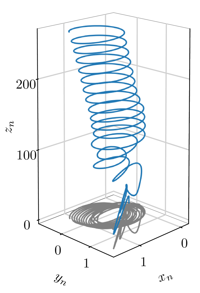
((c)) Case 16: $\mathrm{Ga}=500,\pi_{p}=0.001$: SP.

Figure 13: Cases 12, 14 and 16: At $\mathrm{Ga}=400$ and above, two regimes are found: Three dimensional chaos (3DC) and spiraling (SP).

This new regime is found for Case 12 at $\mathrm{Ga}=400$ and $\pi_{p}=0.01$. The spiraling begins after an initial phase, which transforms from planar zig-zagging up until $t_{n}=40$ to a three dimensional movement. After $t_{n}=80$ the projection of the trajectory onto the $xy$ plane resembles an ellipsis closely approaching the shape of a circle with a diameter of $1d_{p}$. The vertical stride between the spiraling iterations is approximately $14.2d_{p}$, resulting in $\mathrm{St}\approx 0.07$. While not matching perfectly with Auguste & Magnaudet, these numbers come close to their spiral diameter $1.3d_{p}$ and Strouhal number of approximately $0.07$ ($13.5d_{p}$ stride).

Case 13 decreases the particle density ratio further to $0.001$ at $\mathrm{Ga}=400$ with the aid of the virtual mass approach. The vertical crest-to-crest distance changes to $14.06d_{p}$, while the Strouhal number stays the same. Equally, the diameter of the spiral varies only to a very minor degree. Zhou & Dušek provided results of an approximately massless sphere at this Galilei number. Its trajectories match ours, however pitch ($12.6d_{p}$ theirs, $14.06d_{p}$ ours) and terminal vertical velocity ($1.382$ theirs, $1.466$ ours) differ to a certain degree.

Continuing with Case 14, we observe the emergence of a three dimensional chaotic region, simulated here using a Galilei number of $500$ and density ratio of $0.5$. This path is highly irregular and shows no sign of periodicity (Figure 13(b)). The occurrence of 3DC trajectories at this parameter combination was also observed by Auguste & Magnaudet and Zhou & Dušek.

Case 15 features a particle of density ratio $0.05$ and Galilei number $500$. Again, the particle takes up a SP path, albeit with an increased duration of the initial transition compared to the particle of Cases 12 and 13 at $\mathrm{Ga}=400$. Even though at $\pi_{p}=0.001$, Figure 13(c) shows approximately the same delay as $\pi_{p}=0.05$. The vertical stride of the spiral reduces slightly to $13.8d_{p}$ at a horizontal displacement of $1d_{p}$, which is reflected in an increased Strouhal number $\mathrm{St}=0.067$. In this instance, no reference data is available for a direct comparison. Zhou & Dušek performed two simulations at the same Galilei number and density ratios of $0.1$ and $0$; their depicted trajectory of $\pi_{p}=0.1$ reflected the notion of the present transient from planar zig-zagging to a spiralling path. Their resulting Reynolds number of $750$ confirms ours at $\real\approx 757$. After entering the quasi-steady state, the particle of Case 15 moves vertically with $u_{z,n}=1.512$, which places close to Zhou & Dušek’s at $1.406$ ($\pi_{p}=0$) and $1.501$ ($\pi_{p}=0.1$). Radius and pitch of the trajectory closely approach Zhou & Dušek’s as well.

Case 16 displays a modification of the SP trajectory (Figure 13(c)), where the particle at $\pi_{p}=0.001$ and $\mathrm{Ga}=500$ takes up a slightly inclined spiraling path (inclination angle $\approx 0.2\degree$). Such behavior is also observed by Auguste & Magnaudet, who found the corresponding motion already at $\pi_{p}=0.01$. The spiral is described by a diameter of $1.09d_{p}$ and vertical stride of $13.22d_{p}$; the movement along this spiral by $\mathrm{St}=0.074$ and $u_{z,t}=1.455$.

Figure 14: Case 15: Vortices behind a sphere of density ratio $0.05$ at $\mathrm{Ga}=500$. In frames 4 and 5 the three vortex threads delivering a constant torque to the ascending sphere are well visible. A Q criterion threshold of $10^{-10}$ is employed and coloring is done by normalized vorticity, which ranges between -10 (blue) and 10 (red). Lighter colors correspond to stronger magnitude.

6 Conclusion

In this work, we present an improved LBM for simulations of light particles submerged in a fluid, including a comparison with previously established methods. This is based on a set of benchmarks that are chosen to expose specific difficulties and peculiarities arising in systems of submerged particles with density ratios $\ll 1$. In order to achieve stable simulations without excessively fine resolution, we adapt and apply the virtual mass approach of Schwarz et al.⁴⁵, resulting in the improved VM-MEM-LBM. The underlying idea is to artificially increase the mass of the particle to avoid an otherwise vansihing denominator that would amplify inaccuracies of the fluid-particle coupling scheme. This is exactly compensated by an appropriate force and torque, which in practice requires an approximation of the spheres translational and rotational acceleration. This approach is shown to enable density ratios of 0.001 and which would thus permit e.g. the simulation of spherical air bubbles in water. The numerical stabilization scheme is validated both with respect to the accuracy of rotational and translational velocities.

In order to further increase the computational efficiency of the parallel LBM code, we employ adaptive grid refinement. This ensures an adequate and accurate representation of the flow features while permitting large computational domains. Areas in need of refinement are identified by employing sensors evaluating the state of the fluid and the solid phase. The evaluation of the grid adaptation criteria is invoked at regular time intervals. For the case of a rising sphere, the computational cost could be reduced by a factor of 71, when compared to executing same simulation scenario on a uniform fine grid. This is achieved while the accuracy is essentially unaffected.

The efficiency improvement supplied by the adaptive grid refinement algorithm is finally applied in 16 distinct simulation scenarios that study the trajectories of a single rising sphere. In the cases of smallest density ratio of $0.001$, the virtual mass approach proved to be essential to reach a stable time stepping. A multitude of different trajectory types is observed and the results are compared to data from the literature. This includes trajectory classes such as vertical to oblique, zig-zagging, spiraling, three dimensional chaos, and intermittent motion. In many cases good agreement to experimental and numerical studies could be found, for the broad classification via the regimes but also for specific parameters like terminal rising velocities and oscillation frequencies. This served as a further validation of the here presented approach and showcased its applicability for predictions of complex particle dynamics. In some cases, the existing literature provided contradicting statements regarding the observed regime of motion and we observed supporting arguments for one or the other.

We note that while validated here for single spherical particles, our new method is neither restricted to a single particle nor to spherical shapes. The VM-MEM-LBM is also suitable for a wide range of physical parameters, and it can be employed in domains of arbitrary shape. This is considered a major improvement to the numerical schemes applied previously in the simulation studies of trajectories of rising particles. A massively parallel and efficient implementation is available in the open-source waLBerla framework³², enabling the simulation of ensembles of several submerged particles and to study their collective motion. Such studies will be the topic of future research.

References

- 1 Andrady AL. Microplastics in the marine environment. Marine Pollution Bulletin 2011; 62(8): 1596 - 1605. doi: https://doi.org/10.1016/j.marpolbul.2011.05.030
- 2 Wright SL, Thompson RC, Galloway TS. The physical impacts of microplastics on marine organisms: a review.. Environmental pollution (Barking, Essex : 1987) 2013; 178: 483–492. doi: 10.1016/j.envpol.2013.02.031
- 3 Cole M, Lindeque P, Halsband C, Galloway TS. Microplastics as contaminants in the marine environment: A review. Marine Pollution Bulletin 2011; 62(12): 2588–2597. doi: 10.1016/j.marpolbul.2011.09.025
- 4 Driedger AG, Dürr HH, Mitchell K, Van Cappellen P. Plastic debris in the Laurentian Great Lakes: A review. Journal of Great Lakes Research 2015; 41(1): 9–19. doi: 10.1016/j.jglr.2014.12.020
- 5 Thorpe SA, Hall AJ. Bubble clouds and temperature anomalies in the upper ocean. Nature 1988; 328(6125): 48–51. doi: 10.1038/328048a0
- 6 Weller RA. Not so quiet on the ocean front. Nature 1990; 348(6298): 199–200. doi: 10.1038/348199a0
- 7 Alméras E, Risso F, Roig V, Cazin S, Plais C, Augier F. Mixing by bubble-induced turbulence. Journal of Fluid Mechanics 2015; 776: 458–474. doi: 10.1017/jfm.2015.338
- 8 Mathai V, Huisman SG, Sun C, Lohse D, Bourgoin M. Enhanced dispersion of big bubbles in turbulence. 2018(1): 1–6.
- 9 Mathai V, Lohse D, Sun C. Bubbly and Buoyant Particle-Laden Turbulent Flows. Annual Review of Condensed Matter Physics 2020; 11(1): 529–559. doi: 10.1146/annurev-conmatphys-031119-050637
- 10 Bourgoin M, Xu H. Focus on dynamics of particles in turbulence. New Journal of Physics 2014; 16. doi: 10.1088/1367-2630/16/8/085010
- 11 Mathai V, Zhu X, Sun C, Lohse D. Flutter to tumble transition of buoyant spheres triggered by rotational inertia changes. Nature Communications 2018; 9(1): 1–7. doi: 10.1038/s41467-018-04177-w
- 12 Murrow H, Henry R. Self-Induced Balloon Motions. Journal of Applied Meteorology and Climatology 1964; 4(1): 131–138. doi: 10.1175/1520-0450(1965)004<0131:SIBM>2.0.CO;2
- 13 Scoggins JR. Aerodynamics of spherical balloon wind sensors. Journal of Geophysical Research 1964; 69(4): 591–598. doi: 10.1029/jz069i004p00591
- 14 Lugt H. Autorotation. Annual Review of Fluid Mechanics 1983; 15: 123–147. doi: 10.1146/annurev.fl.15.010183.001011
- 15 Jenny M, Dušek J, Bouchet G. Instabilities and transition of a sphere falling or ascending freely in a Newtonian fluid. Journal of Fluid Mechanics 2004; 508(508): 201–239. doi: 10.1017/S0022112004009164
- 16 Biesheuvel A, Veldhuis C. An experimental study of the regimes of motion of spheres falling or ascending freely in a Newtonian fluid. International Journal of Multiphase Flow 2007; 33(10): 1074–1087. doi: 10.1016/j.ijmultiphaseflow.2007.05.002
- 17 Horowitz M, Williamson CH. The effect of Reynolds number on the dynamics and wakes of freely rising and falling spheres. Journal of Fluid Mechanics 2010; 651: 251–294. doi: 10.1017/S0022112009993934
- 18 Ostmann S, Chaves H, Brücker C. Path instabilities of light particles rising in a liquid with background rotation. Journal of Fluids and Structures 2017; 70: 403–416. doi: 10.1016/j.jfluidstructs.2017.02.007
- 19 Zhou W, Dušek J. Chaotic states and order in the chaos of the paths of freely falling and ascending spheres. International Journal of Multiphase Flow 2015; 75: 205–223. doi: 10.1016/j.ijmultiphaseflow.2015.05.010
- 20 Auguste F, Magnaudet J. Path oscillations and enhanced drag of light rising spheres. Journal of Fluid Mechanics 2018; 841: 228–266. doi: 10.1017/jfm.2018.100
- 21 Versteeg HK, Malalasekera W. An introduction to computational fluid dynamics: the finite volume method. Pearson education . 2007.
- 22 F. Moukalled, L. Mangani MD. The Finite Volume Method in Computational Fluid Dynamics. 113. Springer . 2015.
- 23 Chen S, Doolen GD. Lattice Boltzmann Method for Fluid Flows. Annual Review of Fluid Mechanics 1998; 30(1): 329–364. doi: 10.1146/annurev.fluid.30.1.329
- 24 Aidun CK, Clausen JR. Lattice-boltzmann method for complex flows. Annual Review of Fluid Mechanics 2010; 42: 439–472. doi: 10.1146/annurev-fluid-121108-145519
- 25 Clift R, Grace JR, Weber M. Bubbles, Drops, and Particles . 1978.
- 26 Rettinger C, Godenschwager C, Eibl S, et al. Fully Resolved Simulations of Dune Formation in Riverbeds. In: Kunkel JM, Yokota R, Balaji P, Keyes D. , eds. High Performance ComputingSpringer International Publishing; 2017; Cham: 3–21
- 27 Vowinckel B, Biegert E, Luzzatto-Fegiz P, Meiburg E. Consolidation of freshly deposited cohesive and noncohesive sediment: Particle-resolved simulations. Phys. Rev. Fluids 2019; 4: 074305. doi: 10.1103/PhysRevFluids.4.074305
- 28 Peng C, Ayala OM, Wang LP. A direct numerical investigation of two-way interactions in a particle-laden turbulent channel flow. Journal of Fluid Mechanics 2019; 875: 1096–1144. doi: 10.1017/jfm.2019.509
- 29 Benseghier Z, Cuéllar P, Luu LH, Bonelli S, Philippe P. A parallel GPU-based computational framework for the micromechanical analysis of geotechnical and erosion problems. Computers and Geotechnics 2020; 120: 103404. doi: 10.1016/j.compgeo.2019.103404
- 30 Götz J, Iglberger K, Feichtinger C, Donath S, Rüde U. Coupling multibody dynamics and computational fluid dynamics on 8192 processor cores. Parallel Computing 2010; 36(2): 142 - 151. doi: 10.1016/j.parco.2010.01.005
- 31 Hasert M, Masilamani K, Zimny S, et al. Complex fluid simulations with the parallel tree-based Lattice Boltzmann solver Musubi. Journal of Computational Science 2014; 5(5): 784 - 794. doi: 10.1016/j.jocs.2013.11.001
- 32 Bauer M, Eibl S, Godenschwager C, et al. WALBERLA: A block-structured high-performance framework for multiphysics simulations. Computers and Mathematics with Applications 2020. doi: 10.1016/j.camwa.2020.01.007
- 33 Ladd AJ. Numerical Simulations of Particulate Suspensions Via a Discretized Boltzmann Equation. Part 1. Theoretical Foundation. Journal of Fluid Mechanics 1994; 271: 285–309. doi: 10.1017/S0022112094001771
- 34 Aidun CK, Lu Y, Ding EJ. Direct analysis of particulate suspensions with inertia using the discrete Boltzmann equation. Journal of Fluid Mechanics 1998; 373: 287–311. doi: 10.1017/S0022112098002493
- 35 Rettinger C, Rüde U. A comparative study of fluid-particle coupling methods for fully resolved lattice Boltzmann simulations. Computers and Fluids 2017; 154: 74–89. doi: 10.1016/j.compfluid.2017.05.033
- 36 Ladd AJC. Numerical simulations of particulate suspensions via a discretized Boltzmann equation. Part 2. Numerical results. Journal of Fluid Mechanics 1994; 271: 311–339. doi: 10.1017/S0022112094001783
- 37 Uhlmann M. An immersed boundary method with direct forcing for the simulation of particulate flows. Journal of Computational Physics 2005; 209(2): 448–476. doi: 10.1016/j.jcp.2005.03.017
- 38 Kempe T, Fröhlich J. An improved immersed boundary method with direct forcing for the simulation of particle laden flows. Journal of Computational Physics 2012. doi: 10.1016/j.jcp.2012.01.021
- 39 Breugem WP. A second-order accurate immersed boundary method for fully resolved simulations of particle-laden flows. Journal of Computational Physics 2012; 231(13): 4469–4498. doi: 10.1016/j.jcp.2012.02.026
- 40 Inamuro T, Ogata T, Tajima S, Konishi N. A lattice Boltzmann method for incompressible two-phase flows with large density differences. Journal of Computational Physics 2004; 198(2): 628–644. doi: 10.1016/j.jcp.2004.01.019
- 41 Apte SV, Finn JR. A variable-density fictitious domain method for particulate flows with broad range of particle-fluid density ratios. Journal of Computational Physics 2013; 243: 109–129. doi: 10.1016/j.jcp.2012.12.021
- 42 Banks J, Henshaw W, Schwendeman D, Tang Q. A stable partitioned FSI algorithm for rigid bodies and incompressible flow in three dimensions. Journal of Computational Physics 2018; 373: 455-492. doi: 10.1016/j.jcp.2018.06.072
- 43 Jenny M, Dušek J. Efficient numerical method for the direct numerical simulation of the flow past a single light moving spherical body in transitional regimes. Journal of Computational Physics 2004; 194(1): 215–232. doi: 10.1016/j.jcp.2003.09.004
- 44 Hu HH, Patankar NA, Zhu MY. Direct Numerical Simulations of Fluid-Solid Systems Using the Arbitrary Lagrangian-Eulerian Technique. Journal of Computational Physics 2001; 169(2): 427–462. doi: 10.1006/jcph.2000.6592
- 45 Schwarz S, Kempe T, Fröhlich J. A temporal discretization scheme to compute the motion of light particles in viscous flows by an immersed boundary method. Journal of Computational Physics 2015; 281: 591–613. doi: 10.1016/j.jcp.2014.10.039
- 46 Rettinger C, Rüde U. An efficient four-way coupled lattice Boltzmann - discrete element method for fully resolved simulations of particle-laden flows. 2020: 1–37.
- 47 Krüger T, Kusumaatmaja H, Kuzmin A, Shardt O, Silva G, Viggen EM. The lattice Boltzmann method. Springer . 2017
- 48 Qian YH, D’Humières D, Lallemand P. Lattice bgk models for navier-stokes equation. Epl 1992; 17(6): 479–484. doi: 10.1209/0295-5075/17/6/001
- 49 He X, Luo LS. Lattice Boltzmann model for the incompressible Navier–Stokes equation. Journal of Statistical Physics 1997; 88(3-4): 927–944. doi: 10.1023/B:JOSS.0000015179.12689.e4
- 50 D’Humières D, Ginzburg I, Krafczyk M, Lallemand P, Luo LS. Multiple-relaxation-time lattice Boltzmann models in three dimensions. Philosophical Transactions of the Royal Society A: Mathematical, Physical and Engineering Sciences 2002; 360(1792): 437–451. doi: 10.1098/rsta.2001.0955
- 51 Dünweg B, Schiller UD, Ladd AJC. Statistical mechanics of the fluctuating lattice Boltzmann equation. Phys. Rev. E 2007; 76: 036704. doi: 10.1103/PhysRevE.76.036704
- 52 Ginzburg I, Verhaeghe F, D’Humières D. Two-relaxation-time Lattice Boltzmann scheme: About parametrization, velocity, pressure and mixed boundary conditions. Communications in Computational Physics 2008; 3(2): 427–478.
- 53 Khirevich S, Ginzburg I, Tallarek U. Coarse- and fine-grid numerical behavior of MRT/TRT lattice-Boltzmann schemes in regular and random sphere packings. Journal of Computational Physics 2015; 281: 708 - 742. doi: 10.1016/j.jcp.2014.10.038
- 54 Preclik T, Rüde U. Ultrascale simulations of non-smooth granular dynamics. Computational Particle Mechanics 2015; 2(2): 173–196. doi: 10.1007/s40571-015-0047-6
- 55 Wen B, Zhang C, Tu Y, Wang C, Fang H. Galilean invariant fluid-solid interfacial dynamics in lattice Boltzmann simulations. Journal of Computational Physics 2014; 266: 161–170. doi: 10.1016/j.jcp.2014.02.018
- 56 Dorschner B, Chikatamarla S, Bösch F, Karlin I. Grad’s approximation for moving and stationary walls in entropic lattice Boltzmann simulations. Journal of Computational Physics 2015; 295: 340 - 354. doi: 10.1016/j.jcp.2015.04.017
- 57 Hölzer A, Sommerfeld M. New simple correlation formula for the drag coefficient of non-spherical particles. Powder Technology 2008; 184(3): 361–365. doi: 10.1016/j.powtec.2007.08.021
- 58 Tavanashad V, Subramaniam S. Fully resolved simulation of dense suspensions of freely evolving buoyant particles using an improved immersed boundary method. International Journal of Multiphase Flow 2020; 132: 103396. doi: 10.1016/j.ijmultiphaseflow.2020.103396
- 59 Schornbaum F, Rüde U. Massively parallel algorithms for the lattice Boltzmann method on nonuniform grids. SIAM Journal on Scientific Computing 2016; 38(2): C96–C126. doi: 10.1137/15M1035240
- 60 Rohde M, Kandhai D, Derksen JJ, Akker v. dHE. A generic, mass conservative local grid refinement technique for lattice-Boltzmann schemes. International Journal for Numerical Methods in Fluids 2006; 51(4): 439–468. doi: 10.1002/fld.1140
- 61 Schornbaum F, Rüde U. Extreme-scale block-structured adaptive mesh refinement. SIAM Journal on Scientific Computing 2018; 40(3): C358–C387. doi: 10.1137/17M1128411
- 62 Crouse B, Rank E, Krafczyk M, Tölke J. A LB-based approach for adaptive flow simulations. International Journal of Modern Physics B 2003; 17(1-2): 109–112. doi: 10.1142/s0217979203017163
- 63 Yuan R, Zhong C. An immersed-boundary method for compressible viscous flows and its application in the gas-kinetic BGK scheme. Applied Mathematical Modelling 2018; 55: 417–446. doi: 10.1016/j.apm.2017.10.003
- 64 Deister F, Hirschelt EH. Adaptive cartesian/prism grid generation and solutions for arbitrary geometries. 37th Aerospace Sciences Meeting and Exhibit 1999(c). doi: 10.2514/6.1999-782
- 65 De Zeeuw D. A quadtree-based adaptively-refined Cartesian-grid algorithm for solution of the Euler equations. PhD thesis. 1993
- 66 Hunt J, Wray A, Moin P. Eddies, streams, and convergence zones in turbulent flows. Center for Turbulence Research, Proceedings of the Summer Program 1988(1970): 193–208.
- 67 Jenny M, Bouchet G, Dušek J. Nonvertical ascension or fall of a free sphere in a Newtonian fluid. Physics of Fluids 2003; 15(1): L9–L12. doi: 10.1063/1.1529179